| Issue |
A&A
Volume 710, June 2026
|
|
|---|---|---|
| Article Number | A107 | |
| Number of page(s) | 13 | |
| Section | The Sun and the Heliosphere | |
| DOI | https://doi.org/10.1051/0004-6361/202557120 | |
| Published online | 04 June 2026 | |
Hard X-ray sources from the high corona are an integral part of solar eruptions
1
Institute for Data Science, University of Applied Sciences and Arts Northwestern Switzerland (FHNW), Bahnhofstrasse 6, 5210, Windisch, Switzerland
2
Institute for Space-Earth Environmental Research, Nagoya University, Nagoya, 464-8601, Japan
3
Space Sciences Laboratory, University of California, 7 Gauss Way, 94720, Berkeley, USA
★ Corresponding author.
Received:
5
September
2025
Accepted:
9
January
2026
Abstract
Context. Hard X-ray bremsstrahlung emissions are strong diagnostics of electron acceleration during the magnetic energy release process that drives solar flares. Solar Orbiter’s unique vantage point away from the Earth-Sun line allows us to use limb occultation as a diagnostic tool to investigate faint hard X-ray source located above the main flare site that are generally lost in the dynamic range of hard X-ray telescopes.
Aims. We aim to highlight the feasibility and the diagnostic power of limb occultation with Solar Orbiter/STIX to quantify the intensity, spectral shape, and location of the occulted signals relative to the main flare emissions to investigate the energetic importance of nonthermal electrons in the high corona.
Methods. We report on a single event study of the GOES M6 flare on October 19, 2024, simultaneously observed by ASOS/HXI, Fermi/GBM, and Solar Orbiter/STIX. We used standard X-ray spectral fitting tools available through OSPEX to compare the photon spectra observed by the three different observatories. In a second step, HXI and STIX X-ray images were compared to UV and EUV images seen by SDO/AIA to investigate the location of the occulted sources within the flare geometry.
Results. From Earth’s perspective, the flare was seen on-disk near the west limb, while for STIX the flare is occulted by ∼19 degrees, allowing STIX to detect a much fainter thermal and nonthermal source in the high corona related to the coronal mass ejection (CME) associated with the flare. The nonthermal hard X-ray flux indicates that about 5% of flare-accelerated electrons are injected upward into the CME, assuming a thick target model, while the fraction increases for a partially thick target interpretation. The thermal source is hot (23.5 ± 0.7 MK) and expands together with the CME. Even though the thermal source from the high corona has a weak bremsstrahlung signal, due to its large volume, its thermal energy content is on the same order of magnitude as the energy content in the main flare loops. Hence, hard X-ray sources associated with the escaping CME are an important signature of the energy release process.
Conclusions. These observations highlight that high coronal sources are an integral part of solar eruptive events and are energetically important despite their intrinsically faint appearance. For future instrumentation, an emphasis should be put on high-dynamic-range imaging, such as that provided by hard X-ray focusing optics telescopes, to be able to simultaneously observe the flare and the high-coronal sources from a single vantage point observatory.
Key words: Sun: corona / Sun: coronal mass ejections (CMEs) / Sun: flares / Sun: X-rays / gamma rays
© The Authors 2026
 Open Access article, published by EDP Sciences, under the terms of the Creative Commons Attribution License (https://creativecommons.org/licenses/by/4.0), which permits unrestricted use, distribution, and reproduction in any medium, provided the original work is properly cited.
This article is published in open access under the Subscribe to Open model. This email address is being protected from spambots. You need JavaScript enabled to view it. to support open access publication.
1. Introduction
Solar flares are driven by a sudden release of magnetic energy that has been built up in the solar corona over the previous hours to days (for a review of solar flare observations, see Benz 2017). A significant fraction of the released energy is initially going into the acceleration of particles, with energies reaching into the relativistic range. In a second step, these nonthermal particles lose their energy in collisions in the chromosphere. As a result, plasma is heated and rises up into the corona, forming hot, dense flare loops. However, not all electrons end up in the chromosphere: some are ejected upward from the acceleration site. Depending on the magnetic connectivity, these upward-directed field lines go straight out into interplanetary space or they can be part of the coronal mass ejection (CME).
Hard X-ray observations provide strong diagnostics of flare-accelerated electrons (e.g., Fletcher et al. 2011; Kontar et al. 2011) showing prominent bremsstrahlung emissions from the chromosphere as the nonthermal electrons interact with the rather dense ambient plasma. Bremsstrahlung emissions from the same electrons in the corona must be present as well, but it is much fainter due to the low density of the corona (see the review by Krucker et al. 2008). Hard X-ray observations therefore frequently only show the bright chromospheric footpoints, but faint emissions from the corona are lost in the dynamic range of the observations. Limb occultation has been extensively used in the past to block out the bright footpoint emission (e.g., Frost & Dennis 1971; Roy & Datlowe 1975; Hudson et al. 1982; Kane et al. 1992; Tomczak 2001; Krucker et al. 2010; Ackermann et al. 2017; Effenberger et al. 2017). Such observations clearly show that coronal bremsstrahlung emission from flare-accelerated electrons are present in essentially all flares (e.g., Krucker et al. 2008; Effenberger et al. 2017). However, for limb-occulted events, the properties of the main flare sources generally remains unknown. A few examples of HXR flare observations from two different vantage points are available to compare both signals (e.g., Suzuki 1982; Kane et al. 1992), but the diagnostic power of these observations are limited due to the lack of imaging information and the limited spectral coverage and resolution. The Solar Orbiter mission (Müller et al. 2020) with its vantage point away from the Earth-Sun line combined with Earth-orbiting observatories provides for the first time a systematic view of occulted flares at much improved spectral resolution in combination with imaging (e.g., Pesce-Rollins et al. 2024; Hayes et al. 2024). This paper is an initial analysis of a single flare simultaneously observed by the Spectrometer Telescope for Imaging X-rays (STIX; Krucker et al. 2020) with simultaneous coverage by and Hard X-ray Imager (HXI; Zhang et al. 2019) on board the Advanced Space-based Solar Observatory (ASO-S; Gan et al. 2019), which should be followed by a statistical study using the same instruments.
The degree of occultation θocc is generally defined as how many degrees the chromospheric footpoints are behind the limb. In the past, the degree of occultation often had to be guessed by comparing flare locations within the same active region when the active region was seen on-disk. Consequently, the occultation angle was not well known. With Solar Orbiter STIX observations joint with observations from Earth, we have the ability to determine the degree of occultation and we can even compare the difference of θocc of individual locations on flare ribbons.
The degree of occultation can also be expressed in occultation height hocc giving the radial distance normal above the photosphere that is blocked by the solar limb:
 (1)
(1)
where rsun is the solar radius. In this definition, hocc gives the occulted length radial above the flare site. For some considerations, the shortest distance of the occultation docc from the flare site normal to the tangential to the solar limb is preferred, which is reduced by a factor of cos(θocc).
 (2)
(2)
Small occultation angles are less useful as a diagnostic as the upper part of the chromospheric X-ray sources might still be visible. For an occultation angles of 6 degrees, the occultation height becomes 3.8 Mm. Such a height should be generally enough to block footpoint sources, but this depends from flare to flare. Observations of footpoint source altitudes give values as low as a few hundred kilometers (Martínez Oliveros et al. 2012) and values of between 0.8 and 1.7 Mm (Battaglia & Kontar 2011; Krucker et al. 2015). In any case, observations with small occultation angles of below ∼6 degree are tricky to interpret as it will be difficult to prove that indeed the entire radial extent of the footpoint sources are blocked. With the footpoints occulted, faint emissions from the corona becomes the brightest nonthermal component allow us to study the coronal acceleration region in solar flares (e.g., “above-the-loop-top sources”). For the most intense events, observations reveal that the above-the-loop-top sources contain a highly energized plasma with a particle distribution far away from the thermal equilibrium where all particles within the above-the-loop-top source gained energy due to the energy release process (e.g., Krucker et al. 2010; Fleishman et al. 2022). For less intense flares, the fraction of energized electrons is generally lower (e.g., Volpara et al. 2024).
To also block the thermal flare loops, significant larger occultation angles are needed. From statistical studies (e.g., Warmuth & Mann 2013, Fig. 2), loop lengths over a range from 5 to 40 Mm are reported. To have an occultation height of 40 Mm, an occultation angle of about 20 degree is required. In the case in which there are observations available that actually show the flare loop, the required occultation height to block the thermal loop can be approximated rather accurately. For events where the entire flare emission is occulted, nonthermal electrons injected into the magnetic structure of the CME can be observed (e.g., Hayes et al. 2024) or nonthermal emission from the escaping electrons might be detected (e.g., Saint-Hilaire et al. 2009). Most of the published work on hard X-ray sources in highly occulted flares report emission from nonthermal electrons with are injected into the expanding CME (for a list of published flares, see the table in Lastufka et al. 2019). Several of those events additionally report a hot (∼20 to ∼30 MK) thermal plasma escaping within the CME (e.g., Hayes et al. 2024). This hot component is at least partially produced by the energy losses of the nonthermal electrons injected into the CME (e.g., Glesener et al. 2013).
In summary, there are two main ranges for limb-occulted observations to give unambiguous diagnostics: for moderate occultation angles (above ∼6 degrees up to maybe 10–15 degrees), the footpoints are occulted and coronal emissions from the flare loop or above-the-flare loop can be studied. For large occultation, the flare is essentially not visible and faint sources associated with the CME can be investigated. In our initial work on STIX occulted flares, we present a case of the latter kind.
2. Observations
The Spectrometer/Telescope for Imaging X-rays (STIX; Krucker et al. 2020) is an imaging spectrometer in the 4–150 keV energy range on board the Solar Orbiter missions. STIX has been operating for over four years with essentially continuous data acquisition. STIX had recorded over 85 000 flares by August 2025, including hundreds of M class flares. Considering that about 10% of all flares are partially limb-occulted (the good zone for occultation is about 10 degrees on either side compared to 180 degrees of coverage for on-disk flares, for each of the two categories), there is an extensive database of occulted flares waiting to be analyzed.
As the occulted emission have rather weak fluxes, only large flares (M class and above) generally show strong enough occulted emission to allow a detailed spectral and imaging analysis. Here we report on an GOES M6 flare (SOL2024-10-19T06 observed from 0.48 AU) with a high degree of occultation (θocc = 19°) for STIX, so that the flare loops is fully blocked. The event was selected as it has good coverage from three hard X-ray observatories (STIX, HXI, and Fermi Gamma-ray Burst Monitor (GBM; Meegan et al. 2009) with a clear nonthermal signal in all datasets. In addition, subtracting the non-solar background is rather straightforward for all three observatories. Furthermore, the degree of occultation is high so that only emission from the high corona is seen by STIX. Hence, this flare is an ideal candidate to search for secondary X-ray sources in the high corona.
In the next subsections, the following order of topics are addressed:
-
The degree of limb-occulation of the STIX observations;
-
The relative evolution of X-ray time profiles;
-
Spectral fitting and determination of the relative strength of the occulted nonthermal signal;
-
Imaging results in UV, EUV, and X-rays taken from Earth and Solar Orbiter vantage points.
2.1. Flare location and degree of occultation
SOL2024-10-19T06 occurred on-disk as seen from Earth with flare ribbons observed by the Atmospheric Imaging Assembly (AIA; Lemen et al. 2012) in UV and by HXI in hard X-ray around S04W83 (see Fig. 1). The flare is associated with a narrow CME at moderate speeds of a few hundred kilometers per second (CACTus CME list; Robbrecht & Berghmans 2004). At the time of the flare, Solar Orbiter was at a radial distance from the Sun of 0.48 AU, 23.6 degrees off the Earth-Sun line to the east, and close to the ecliptic (within 0.8 degrees). This makes the flare limb-occulted from the Solar Orbiter vantage point. For the main flare ribbon with the brightest emissions in UV and HXR, the occultation angle is around 19 degrees. Using the eastern and western most part of the main flare ribbon, we get an occultation angle between 17.9 and 22.0 degrees, or an occultation height between 35.3 and 54.6 Mm. In UV, there is an faint remote brightening to the east of the flare ribbon around [933″,−92″]; see Fig. 1. Even this source is clearly occulted for STIX by 10.6 degrees. Hence, STIX cannot detect any chromospheric signals of the flare by a wide margin.
 |
Fig. 1. Flare location of SOL2024-10-19T06 as seen from Earth by AIA and HXI. The image to the left shows the UV and HXR flare ribbons during the impulsive phase. The flare location is on-disk near the western limb. On the right, the EUV and HXR images at the flare peak time are shown. The AIA 131A image is shown in logarithm scaling to enhance the faint extension to the north that reaches high altitudes. The flare loop itself is saturated in this AIA image and strong diffraction pattern signatures are seen. At a higher order, the shape of flare loops can be seen in the diffraction patterns. The insert on the left figure shows the associated CME as seen by LASCO as a running difference image (from CACTus CME list). In both figures, the orange curve shows the limb as seen from the Solar Orbiter vantage point, indicating that the flare is highly occulted and neither the flare ribbons nor the flare loop can be seen from Solar Orbiter’s vantage point. The high reaching faint loops, on the other hand, are visible from Solar Orbiter. The dashed black curve gives a rough estimate as to the altitude above which the solar corona becomes visible for instruments on board Solar Orbiter. |
The main flare loops are heavily saturated in AIA 131A images and a strong diffraction signal is seen (Fig. 1, right). The diffraction patterns reveal the actual size of the flare loop indicating a rather compact source of about 4″ × 10″. The compact size is confirmed by HXI observations in the thermal range, see Fig. 1. Hence, the main flare loop does not extend above the occultation height by a large margin. Therefore, the main flare loop is also invisible to STIX. In addition to the main flare loop that saturates the AIA image heavily, there is a faint emission from a much larger loop system to the north of the main flare loops (see Fig. 1, right). For STIX, these large loops are partially visible above the solar limb. As these loops are spatially extended beyond the STIX angular resolution coverage, even the coarsest STIX grids are too fine to fully modulate the hard X-ray signal. Hence, STIX can detect these high-altitude loops, but imaging diagnostics will be limited (see Sect. 2.4).
In summary, SOL2024-10-19T06 is highly occulted by the limb from Solar Orbiter’s vantage point. STIX cannot see the main flare site including the footpoints, the main thermal loop, as well as a potential above-the-loop-top source. Hence, the occulted signal detected by STIX is from secondary sources associated with the CME, but not from the main flare loops. In the next section, we discuss the time evolution of the occulted STIX signal relative to the flare profiles seen by GOES, GBM, and HXI.
2.2. X-ray time evolution
Figure 2 compares the GBM, HXI, and STIX nonthermal time profiles with the GOES light curves. All curves have been background subtracted with the pre-flare flux and normalized to the peak value. STIX times have been adjusted by 257.4 s to take into account the closer radial distance of Solar Orbiter compared to Earth at that time. The GOES thermal profiles show a simple shape with an impulsive increase and a slower decay. The GOES short wavelength channel peaks slightly earlier and decays faster indicating the usually observed behavior that the hottest flare temperatures are reached before the peak time of the GOES low wavelength channel. The nonthermal profile from GBM (40–80 keV) and HXI (35–50 keV) show the total flare emission with several nonthermal peaks during the rise in the thermal emission seen by GOES. The two curves agree well at first glance (a quantitative comparison will be presented in the following section). In summary, the flare is a standard example of a flare, with an impulsive phase of a few minutes duration followed by a decay phase, without any further nonthermal bursts during the decay.
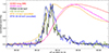 |
Fig. 2. X-ray time evolution of SOL2024-10-19T06: Background-subtracted and normalized X-ray profiles are shown from GOES, GBM, HXI, and STIX. For GOES, GBM, and HXI, the entire flare emission is seen, while for STIX the profiles are strongly affected by limb occultation. |
The profiles from STIX are different due to the partial limb occultation. The nonthermal (20–50 keV) profile from STIX looks nevertheless similar in duration and shows the same main peaks as seen in the total flare profile by GBM and HXI, although the dip between the first and second peak is less pronounced. It is obvious that the STIX signal is much noisier, indicating that it sees a smaller fraction of the total signal. The thermal profile from STIX, however, is different, with an initial peak that reaches a maximum at the end of the main nonthermal burst. This behavior follows the same trend as reported by Glesener et al. (2013) in SOL2010-11-03T where the nonthermal profile was interpreted as the heating rate that drives the thermal profile. The first peak is followed by a second less pronounced peak that decays slower than even the GOES long wavelength channel. These differences reflect how STIX does not see the main flare loops due to limb occultation. Before we discuss the imaging results in Sect. 2.4, the relative intensity of the hard X-ray photon spectra are discussed in the following section.
2.3. Forward fitting the individual count spectra
The goal of forward fitting the observed count spectra is to get an estimate of the incoming photon spectra for each instrument. Such an approach is necessary as hard X-ray counts at a fixed energy can be produced by a range of photons above that energy (i.e., the spectral response matrix of X-ray telescopes have significant contribution from non-diagonal elements). The fitting result is a photon spectrum which is in agreement with the observed count spectrum given the knowledge of the spectral response of the instrument. With the photon spectra in hand, we can then compare the relative strength of the total flare signal to the partially occulted signal, as a function of energy.
For spectral fitting, the Object Spectral Executive (OSPEX software; Schwartz et al. 2002) package was used, which has been the standard package for solar HXR spectral fitting over the past decades. We used the SolarSoftWare implementation from December 2024 in combination with the STIX software version v0.5.2. As OSPEX is not set up for joint fitting of multiple datasets, we fit each spectra separately.
-
For GBM, data from each detectors was fit separately. We excluded the most sunward detectors as the count rates are high and pileup effects can distort the spectrum. The detectors used are N0, N2, and N4, using OSPEX detector number definitions.
-
For HXI, we used the three dedicated detectors without imaging grids (using the HXI naming convention, we used detector t1, t2, and t3).
-
For STIX we summed over the 12 detectors with coarse sub-collimators (grid 7 through grids 10; see Krucker et al. 2020) to enhance statistics. We excluded the detectors covered by finer grids as the grid self-calibration was not yet available at the time of the data analysis (STIX GSW version 0.5.2). For more details on the detector selection, we refer to Jeffrey et al. (2024).
Background subtraction of non-flare related signals is a key step in spectral fitting. For this initial paper, an event with a rather simple background time evolution has been selected for which pre-flare background subtraction works well:
-
For GBM taking data in low Earth orbit, background subtraction is generally challenging. However, for SOL2024-10-19, the background variations during the flare can be rather well approximated by using a pre-flare time interval (06:45:22.9-06:47:29.8UT).
-
HXI is also in low Earth orbit, in a polar orbit. For this flare, HXI is near the equatorial region and pre-flare background (06:46:42.6- 06:48:58.6UT) subtraction works well.
-
As a deep-space mission, STIX has an essentially constant background over the timescale of flares, making background subtraction rather straightforward. For this flare we used the non-flaring times (06:48:11.8-06:49:08.7UT) before the flare onset.
Compared to the flare signal, the background starts to dominate above 80 keV for GBM and HXI. For the occulted signal seen by STIX, the background dominates above 28 keV.
A straightforward fitting approach was used with a thermal, a broken power law, and an albedo component, assuming an isotropic emission pattern for the albedo estimation (e.g., Kontar et al. 2006). We did not use the standard thick target model, as the interpretation of the occulted emission as thick target might not necessarily be fulfilled. We therefore used a simpler parametric fit of a power law for the nonthermal component. In any case, to derive the ratio of photon flux, it is in principle not important what kind of fit model we select, as long as the fit model represents the data well. As the albedo component (i.e., photon which are Compton back-scattered in the lower layers of the solar atmosphere) for the STIX signal is blocked by the limb, the albedo component is not used in the fit to the STIX spectra. GBM and HXI, on the other hand, see the albedo component, giving us two options for comparing the photon fluxes: we have the choice to remove the fit albedo component for GBM and HXI and compare the primary component for all instruments, or leave the albedo in and compare the photon spectra as measured by the different observatories. From a physical point of view, the former approach is likely appropriate. For the albedo component, we use the standard isotropic approach in OSPEX. As SOL2024-10-19 is near the limb as seen from GBM and HXI, the albedo component is relatively modest. For flares closer to the disk center, however, the albedo component can be as bright as the primary component. Hence, for a different flares the approach that is used might matter.
We present here a detailed analysis of the spectrum during the first hard X-ray peak. The observed count spectra of the different observatories and the resulting photon spectra are shown in Fig. 3.
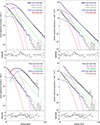 |
Fig. 3. Spectral fitting results for the first hard X-ray peak (06:52:43.1 to 06:52:57.5UT at Earth). The two plots on the top compare STIX with GBM, while the two plots on the bottom compare STIX with HXI. The STIX spectrum is shown in histogram style, while the other two are shown by crosses. For each comparison the count spectrum as well as the photon spectra are shown. Individual fit components are shown in color as indicated by the annotation. |
2.3.1. Thermal spectrum of the total flare
As GBM and HXI fitting of the thermal component is difficult, we did not quantitatively compare the thermal fit results, but instead used the GBM and HXI thermal fit to highlight that the nonthermal component clearly dominates above 20 keV. To get an order of magnitude estimate of the thermal energy content of the flare, we used the emission measure and temperature derived from GOES with the volume estimated from AIA 131A. During the first nonthermal peak investigated in detail here, we get a GOES temperature of 17.5 MK (EM = 4.6 × 1048 cm−3). Together with the area of ∼4″ × 10″ derived from AIA 131A observations, we get a volume on the order of 6 × 1025 cm−3. This results in a flare loop density of 2 × 1011 cm−3 and an order of magnitude thermal energy content of 2 × 1029 erg (note that these are the values at the first hard X-ray peak, not at the GOES peak time). These are all plausible values for an M6 flare.
2.3.2. Nonthermal spectrum of the total flare
The HXI and GBM photon spectra agree within 8% above 20 keV (Fig. 4): a satisfactory result considering the current stage of the available calibration. The fit power law slopes derived from the two instruments agree well within the error bars given values of γ = 4.90 ± 0.12 and γ = 4.88 ± 0.06 for HXI and GBM, respectively. The error bars given are the standard deviation of the power indices obtained from the different detectors. The error bars obtained from the fit procedure itself are generally smaller, indicating, as was expected, that systematic effects contribute to the overall scatter in the results of different detectors. Nevertheless, the two measurements agree well within expected error bars. Compared to the statistical study of flare nonthermal emissions by Battaglia et al. (2005), SOL2024-10-19T06 has an average nonthermal component within the reported distribution.
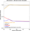 |
Fig. 4. Comparison of the GMB, HXI, and STIX photon spectra shown in Fig. 3. The thin gray and black lines give ratios of individual detector pairs for HXI and GBM, respectively, while the orange curve represents the ratio between the averaged GBM and HXI photon spectra. As GBM and HXI both see the full flare emission, the ratio should be 1 for perfectly calibrated instruments. Above 20 keV, the ratio is close to unity indicating a satisfactory state of the calibration has been achieved to date. At lower energy, the deviations from unity are significant reflecting that these low energies are much more difficult to calibrate. As STIX detects only part of the total flare signal due to occultation, a ratio of less than one is expected. The ratio above 20 keV is observed to be around 4%. Surprisingly, the ratio stays constant with energy indicating the same spectral shape for the high-coronal sources as for the total flare. |
2.3.3. Nonthermal spectrum from the high corona
As was expected, the nonthermal component observed by STIX is much fainter. Compared to the total flare, the emission STIX detects is about 4.2 ± 0.4% of the total flare. If we only compare the primary component (i.e., subtract the albedo component), the fraction become 5.0 ± 0.3%. Considering that this is emission from well above the flare, it is a surprisingly large fraction. Even more surprising is that the ratio is the same even at higher energies. Hence, the STIX spectra has a similar power law slope as the total flare emission with a value of 4.79 ± 0.12. Such a value is slightly harder than the average of a statistical study of occulted RHESSI flares that reports an averaged value of the power law slope of 5.5 with a standard deviation of 1.3 (Krucker & Lin 2008). Nevertheless, it is not a particularly hard spectral slope for an occulted flare. In any case, the simplest scenario with the same electron spectral shape, δ, with thick target emission from the chromosphere (i.e., δ = γ + 1) and thin target emission from the corona (i.e., δ = γ − 1) does not hold at all. We come back to this point of discussion after the imaging results are presented in Sect. 2.5.
2.4. Imaging
X-ray imaging for this flare was done at four time intervals: the onset of the thermal emission as seen by STIX, for the first and second nonthermal peak, and during the second peak in the thermal emission; see Fig. 5 for reference. Standard STIX imaging (software version 0.5.2) was used (Massa et al. 2022, 2023). The STIX images shown in Fig. 5 are reconstructed using the maximum entropy algorithm MEM GE Massa et al. (2020). As the observed modulations of the finest grids are not seen above the noise level, only sub-collimators 5 through 10 have been used in the image reconstruction giving an angular resolution of 29.8″. At the radial distance of Solar Orbiter of 0.48 AU, sources appear about twice as big in angular size compared to Earth. Such a resolution is adequate to study coronal sources. For each time interval, images in the thermal range (4–9 keV) were reconstructed, while for the two interval with nonthermal emissions a second set of images at 18–28 keV were derived. The absolute location of STIX images are currently not well known. We shifted the STIX images by 25″ in a negative heliocentric X direction. Such a shift produces a better match with the optical solar limb location. In any case, the conclusions presented in this paper are not influenced by the uncertainty in location. The image quality of the nonthermal images is moderate and we therefore only show contours above 30%, as lower contours likely contain contribution from imaging reconstruction artifacts.
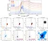 |
Fig. 5. Imaging results from STIX (center row) and from HXI and AIA (bottom row) for four intervals during the flare. The top plot shows the STIX X-ray profiles (normalized and stacked for a clearer display) with the four time intervals marked by numbers. The fields of view of the images have been adjusted to display the same projected area on the Sun to take into account the closer distance of Solar Orbiter to the Sun. The second and fourth time intervals are the same as the ones used in Fig. 1. |
The STIX results are compared to the AIA and HXI images obtained from Earth perspective (see the bottom row of Fig. 5). HXI images were reconstructed using the CLEAN algorithm within the HXI software package (Solar software package Version December 2024). The images shown are the clean map without the residuals added (the current version of the software does not yet provide a clean map with the residuals added). Compared to the backprojection map used as input to CLEAN, the residual maps have remaining peaks up to the 30% level of the peak flux in the backprojection images. As for STIX, we therefore only plot contours above 30%. In the following subsections, we discuss imaging results during the different temporal phases of the flare.
2.4.1. Onset
The STIX source before the start of the impulsive phase is seen at the limb with part of the emission cut by the limb. Spectral fitting indicate a temperature of 15.8 ± 0.4 MK (EM = 3.4 ±0.5 × 1046 cm−3 at 06:51:00UT). Similar temperatures are reported for the onset of flares derived from GOES observations (e.g., Hudson et al. 2021). This STIX temperature and EM translates into a GOES class of B1.0 for the occulted part. Such an estimate is always a lower limit, as plasma at cooler temperatures is weighted higher for GOES than for STIX. The observed GOES flux at that time is C3.6 without subtraction of a non-flaring component. It is not apriori clear how to subtract the part of the GOES flux that does not belong to the flare. Subtracting the flux from before the earliest onset in the STIX signal (06:48:00UT) gives a flare flux of C1.0. However, it is not clear that such a choice for the background subtraction is appropriate. Nevertheless, the STIX emission accounts for about 3 to 10 % of the observed GOES flux. This is a plausible value and it is on the same order of magnitude as the occulted nonthermal signal seen during the impulsive phase.
The AIA 131A image taken around the same time shows an extended source in the same direction as the STIX source potentially reaching altitudes to become visible for Solar Orbiter. As the temperature dependence of AIA 131A peaks around 10 MK, the source structure compared to the STIX 4–9 keV observations are not expected to be exactly the same. We speculate that the STIX source corresponds to the hottest part of the AIA 131A source. The contribution of the STIX source to the 131A can be faint as the STIX derived temperature is significantly hotter than the peak temperature of the 131A channel. With the STIX X-ray source size of 70.3 ± 3.1″ × 27.9 ± 2.7″ (derived from forward fitting the STIX visibilites; Volpara et al. 2022), we derive a volume of ∼3.7 × 1027 cm3 (assuming the volume scales with area to the power of 1.5 and a filling factor of unity). Together with the observed emission measure, this gives a density on the order of 3 × 109 cm−3. This is a plausible density for a high coronal source.
In summary, the STIX onset emission is seen just above the limb from an extended source that is rather hot with a low density. The onset is located to the north of the main flare loop, but the connection to the flare source is not immediately clear.
2.4.2. Impulsive phase
Both hard X-ray peaks show a similar source geometry in the low corona with emissions mainly from the flare ribbons. There is a good correspondence between the UV and HXR sources as expected during the impulsive phase of the flare. The thermal hard X-ray source seen by HXI connects the flare ribbons. Compared to the ribbon location and separation, the thermal emission appears to be from a rather flat loop not reaching an altitude as high as a semicircular loop connecting the flare ribbons. The HXI images show some additional emissions from above the thermal source reminiscent of an above-the-loop-top source (e.g., Masuda et al. 1994). For further interpretations, the next generation of HXI grid calibration needs to be available. In any case, this potential above-the-loop-top source is clearly not visible from the Solar Orbiter vantage point.
The STIX thermal emission during the impulsive phase comes from a similar location as during the onset. At the peak of the thermal emission during the impulsive phase, the fit temperature is T = 23.5 ± 0.7 MK (EM = 17.0 ± 1.6 × 1046 cm−3 at 06:53:31UT). The estimated GOES class for this component is B6, with the observed GOES class at that time being M3.0. Hence, the expected GOES signal of the high coronal source is in the low-percentage range. Compared to the onset, the temperature has clearly increased to a rather hot temperature exceeding the GOES peak temperature of slightly above 20 MK. The increased emission measure and the increased area (78.±2.0″ × 33.9 ± 1.0″ at 0.48 AU; volume of 6 × 1027 cm3) results in a slightly increased density to 5 × 109 cm−3 relative to the source before the onset. Such a low increase is different from what is generally seen in flare loops as heated chromospheric plasma is unlikely to contribute to increasing the density high in the corona. Compared to the main flare loop (see Sect. 2.3.1), the high coronal source has an emission measure that is ∼30 times lower and a volume that is ∼100 times larger. In the calculation of the total energy content in a thermal source,
 (3)
(3)
where k is the Bolzmann constant, the difference in the EM and V of the flare sources relative to the coronal source largely balances out. As a result, the energy content of the coronal source of 3 × 1029 erg is surprisingly larger and on the same order of magnitude as the energy content of the flare loop of 2 × 1029 erg (see Sect. 2.3.1). If the high coronal source has a filling factor q smaller than unity, Veff = qV, the derived energy is smaller by  . For a filling factor of unity, the high coronal source has a similar energy content to the main flare loop. Considering the expected GOES signal is so much fainter, this sounds strange at first glance. However, this reflects bremsstrahlung diagnostics: extended X-ray sources at the same energy content as a compact source radiate much fainter in X-rays as the compact source. Consider two sources at the same temperature with the same energy content, but with different volumes. As the temperatures are the same, the ratio of the resulting GOES flux is proportional to the ratio of the emission measures. As the sources have the same energy content and temperature, they both contain the same number of particles, Ncompact = Nextended, and the ratio GOES fluxes become inversely proportional the ratio of the volumes:
 (4)
(4)
Hence, an extended source radiates much less than a compact source due to how the bremsstrahlung process works even if they contain the same energy content. Bremsstrahlung can be enhanced if the number of particles is increased, but also by an increased ambient density (increasing the density of the targets). This favors compact sources over extended sources. Therefore, the GOES fluxes (as well as any bremsstrahlung flux) are dominated by the compact flare sources and extended sources can get lost in the limited dynamic range of observations despite their energetic importance. Compact flare loops and extended sources in the high-corona as discussed in this paper are examples of this. When only comparing flare loops, this bias is less pronounced, as flare loops generally are all relatively compact. This is why it works to use the GOES class as an approximate measure for the “size” of a flare. Nevertheless, the generally adopted GOES classification is of course also biased by this effect. For flares with the same GOES fluxes, a compact flare contains less thermal energy than a flare with an extended source structure.
The high-coronal thermal source associated with the impulsive phase decays after the nonthermal peak (decay from 06:52:45 to 06:53:15UT; see Fig. 2). Decays of thermal bremsstrahlung sources are driven by cooling of the source, but also by source expansion:
 (5)
(5)
where fbs is the bremsstrahlung flux, g(T) represents the bremsstrahlung dependence on temperature, EM is the emission measure, N is the number of particles, V is the volume of the source, and t denotes the time (e.g., Dennis & Phillips 2024). Conductive losses of the high coronal source are likely low as the cold chromosphere is far away. Furthermore, radiative losses are rather low for such a high-temperature plasma at a rather low density (e.g., Bradshaw & Raymond 2013). Hence, the decay might not necessarily be driven by cooling, but the expansion of the source is an important factor. Over the first minute after the thermal peak (06:53:30UT), the source area expands by about 30%. Hence the volume is changing significantly, and consequently the bremsstrahlung flux decreases. We emphasize the often overlooked importance of source expansion: The bremsstrahlung flux decay of expanding high-coronal sources might not necessarily be due to cooling, but rather due to expansion. While this topic is outside the scope of this paper, it deserves to be addressed in a future quantitative study.
For a discussion of the nonthermal source interpretation, it is helpful to look at the detailed time evolution in hard X-rays and EUV during the impulsive phase (Fig. 6). To highlight the EUV emissions from the high corona, the lower coronal emissions are not shown. The cutoff for flagging has been selected to roughly represent what can be seen from Solar Orbiter’s vantage point. While such an approach is of course not a perfectly accurate representation of what is seen by STIX, it helps put the occulted observations into context.
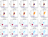 |
Fig. 6. Time evolution during the impulsive phase in ten time steps (STIX times are adjusted to Earth; for a reference of the duration, see the green bar in Fig. 5, top). The cadence was taken from the AIA 131A frames (12 s cadence with a 2.9 second integration time). STIX images were reconstructed around the same time steps as the AIA images with a 12 second integration time to enhance counting statistics. The top ten panels show the STIX observations with thermal images (4–12 keV) shown in a red-colored table and nonthermal images (18–28 keV) are given with blue contours. The contour levels are scaled to the 20, 40, 60, 80% of the maximum emission in the time series. For the last two frames, the nonthermal emission drops below 20% of the maxmimum and therefore no blue contours are seen. The bottom panels show running difference images (AIA 131A) in a blue-colored table, with the dark representing enhanced intensity. To highlight the visibility of the faint EUV emission from the high corona, the low corona has been flagged and set to zero. For reference, the location of the main X-ray flare is shown by the contours; see Fig. 1. |
At the time of the onset of the nonthermal emission, AIA 131A images show that the top of the escaping plasma becomes visible from Solar Orbiter’s vantage point. The STIX thermal sources evolve with the escaping EUV structure and rise and expand in time. By chance, the escaping EUV structure became visible to Solar Orbiter at the start of the impulsive phase. For an even higher degree of occultation, the initial nonthermal peak from the high corona would not have been visible for STIX, but only the later peak when the CME eruption has reached higher altitudes. Hence, this event is a fortunate case with the degree of occultation being at the right level. However, there should be other events in the database for which the start of the impulsive phase is missed. The STIX nonthermal emissions are also associated with the escaping EUV structure and resemble earlier publications (e.g., Hayes et al. 2024). As has been reported previously, the nonthermal source locations are not identical to the thermal sources (e.g., Lastufka et al. 2019, Fig. 2). The quality of the reconstructed images are limited by statistics and it is difficult to draw stringent conclusions on the relative source locations. In any case, SOL2024-10-19 is a further case where the occulted emissions are associated with flare-electrons injected into the escaping CME.
2.4.3. Later thermal phase
For completeness, we also discuss briefly the later phase of the thermal emissions without going into details. During the later phase, the AIA 131A shows the flare loop and an extended loop system reaching high altitudes. The main flare loop dominates the AIA 131A image, with the extended source being much fainter. GOES is dominated by the main flare loops, while the occulted signal sees only the extended loop system. This explains why a different time evolution is seen in the thermal profiles of GOES and STIX (Fig. 2). The hot source is clearly expanding upward with approximate speeds of a few hundred kilometers per second. These speeds are on the same order of magnitude as the reported CME speed, and it is therefore plausible that the hot structure is escaping within the CME (CACTus CME list; Robbrecht & Berghmans 2004).
The spatial extent of the extended source is in excess of 100″ as seen from Earth. From Solar Orbiter’s radial distance from the Sun, the source is about double the angular extent. Hence, STIX imaging is challenged, as the coarsest subcollimator has a resolution of 180″. The coarsest STIX subcollimators indeed detect modulations, but it is also clear that there is a second component of un-modulated flux from a source significantly larger than 180″. Therefore the reconstructed STIX image show only part of the source. To reflect this, the thermal hard X-ray image in Fig. 5 is shown in a gray color table. Nevertheless, it is reasonable to assume that the STIX thermal emission comes from an extended source seen in AIA 131A.
Contrary to imaging, spectral analysis is not affected by the large source sizes seen in the later phase. The temperature at the second thermal peak is 19.2 ± 0.5 MK (EM = 30.6 ± 3.0 × 1046 cm−3 at 06:55:31UT) and deceases in time with an increasing emission measure (14.7 ± 0.3 MK (EM = 59.2 ± 5.3 × 1046 cm−3 at 06:58:31UT). As we do not have a source size estimate, we do not derive a density and an energy content for the later part.
2.5. Discussion on thick versus thin target model
In the previous section, we showed the hard X-ray source in the high corona has a similar spectral shape as what is observed from the footpoints, but the strength of the HXR emission is only about 4%. A simple thick and thin target model for the footpoints and the high coronal source would predict a difference in slope of 2 in the power law index. This is definitely not realized. While it makes sense to use the thick target approximation for the footpoint source, it is remains open which is the better approximation for the coronal source. Depending on the ambient density and the degree of particle trapping, the thick, thin, or an in-between scenario could be realized. Using the derived ambient density of the high-altitude thermal source of 5 × 109 cm−3, the path length to stop 50 keV-electrons becomes l50 ∼ 750 Mm (e.g., Emslie 1978), much larger than the source size of 40 Mm. Nevertheless, if electrons are trapped, it takes only about t50 ∼ 6 s to stop it, much shorter than the duration of the first peak alone of about 18 s. For 100 keV, the values become l100 ∼ 3000 Mm and t100 ∼ 18 s, while for energies below 10 keV, l10 becomes lower than 30 Mm and the thick target is realized. Hence, a range of scenarios are possible. In the following, we first discuss the thin target scenario followed by the thick target version.
2.5.1. Thin target coronal source
The thin target is the extreme case assuming that the ambient density is low enough so that collisions do not significantly lower the energy of energetic electrons. In such a case, the resulting thin target bremsstrahlung emission is inversely proportional to the ambient density. If the density is known, the instantaneous number of flare-accelerated electrons above a cutoff energy can be derived. Thermal density estimates within the nonthermal source are generally difficult to obtain and therefore thin target diagnostics are not as powerful as for the thick target case.
The thermal X-ray emission seen by STIX gives a rough estimate of the ambient density in the energized region in the high corona on the order of 5 × 109 cm−3. At least for the first hard X-ray peak, when the thermal and nonthermal sources appear mainly co-spatial, this density is a plausible value. For the second hard X-ray peak which has a component further to the north, the density might be different. Using a density of 5 × 109 cm−3 and a cutoff energy of 25 keV, the instantaneous number of electrons becomes 2 × 1034 with a total energy content of 8 × 1026 erg. All these values scale inversely with density.
The instantaneous energy content gives the energy in electrons present at a snapshot in time, and therefore it does not represent the total number required to sustain the nonthermal emission for the entire duration (the first peak lasts about 18 s). The shorter electrons stay in the nonthermal source, the more often they need to be replenished, and the required nonthermal energy increases accordingly. To investigate the escape of electrons, we can consider the collisional loss scales. A 25 keV electron has a stopping column density of 9 × 1019 cm. For a density of 5 × 109 cm−3, we get a a mean free path of 2 × 1010 cm, and with the velocity of a 25 keV electrons (0.30 c), we get a collisional lifetime of about 0.6 seconds. To have a thin target scenario realized, the travel time through the X-ray source needs to be much less than the stopping time. Hence, replenishment of accelerated electrons during the 18 second long peak needs to happen much more often than 30 times, and the total energy in nonthermal electrons becomes ≫2 × 1028 erg. The nonthermal energy content in the thin target approximation reaches the same order of magnitude as the nonthermal energy content in footpoints. Furthermore, the electron spectral index is much harder in the high coronal source with a power law slope of around 4, while the footpoints have an index of 6. Hence, if the thin target approximation applies, the nonthermal population in the high corona would have more high-energy electrons than in the flare footpoints. Hence, it is questionable that a thin target scenario is applicable.
2.5.2. Thick target coronal source
We discuss first the energy deposition rate in the main flare ribbons using the thick target approximation. Using a cutoff energy of 25 keV, the energy deposition rate becomes 1.6 ± 0.1 × 1028 erg/s from the fit to the GBM spectrum and 1.8 ± 0.1 × 1028 erg/s from HXI. Integrated over the peak duration of 18 s, the total energy deposition becomes 3 × 1029 erg. This is the same order of magnitude as the thermal energy content (see Sect. 2.4.2). Hence, there is a similar amount of energy in electrons above 25 keV as in the thermal loop. This is similar as observed in the many of flares (e.g Saint-Hilaire & Benz 2005).
As the coronal source has the same spectral shape, but only 5% of the flux compared to the footpoints (after subtraction of the albedo component), the energy in accelerated electrons is 20 times smaller for the coronal source giving 1 × 1028 erg. The nonthermal energy content is significantly lower than the thermal energy content in the above the loop top sources (3 × 1029 erg), at least when using a cutoff of 25 keV. For a cutoff of 9.5 keV, the energy content would be equal. Hence, nonthermal electrons in the high-coronal source can significantly contribute to the heating of plasma ejected within the CME, as has been reported reported by Glesener et al. (2013) for a different flare.
These upward-traveling electrons radiate faintly in hard X-rays as the ambient density is low. To realize the thick target scenario, these electrons would need to encounter a dense plasma. In such a case, the high-coronal thick target emissions would be delayed by the travel time from the accelerator to the location of the dense plasma structure. From the location of the nonthermal source, such a distance (order of magnitude of 40 Mm) is crossed by a 25 keV electron in half a second. Hence, the time profile of the footpoints and the high coronal source would be similar compared to the available cadence of the observations, as observed. Hence, in a scenario with spots of high density within the eruption the thick target scenario could be realized and a similar time evolution and spectral shape of the main flare and high-coronal source is produced. Alternatively, and possibly more likely, the thick target is realized due to trapping of particles within high-coronal source. The trapping times needed for the thick target approximation to be valid are given in Sect. 2.5 (e.g., t50 = 6 s) are significantly shorter than the duration of the impulsive phase of about 100 s. Hence, trapping would smear out the time profiles of the high-coronal sources somewhat, but it would not create an exponential decay after the injection stops.
2.5.3. Conclusions
A thick target scenario is clearly more likely. A thin-target scenario requires a harder injected electron spectrum in the upward direction and the number of electrons needed is very large, making such an interpretation less likely to be realized. The time evolution and the spectral shape clearly favor a common acceleration mechanism for the electron population injected into the chromosphere and upward into the escaping CME, suggesting a thick target scenario for both the upward- and downward-directed components. A thick target scenario in the high corona is plausible given the rather large observed source size and duration of the impulsive phase. Alternatively, over-dense substructures within the source region could produce a thick target.
3. Conclusions
This paper presents a single event analysis of a highly limb-occulted flare detected by the hard X-ray imaging spectrometer STIX on board Solar Orbiter. The Earth-orbiting observatories Fermi/GBM and ASO-S/HXI saw the flare on-disk, allowing us to compare the high-coronal sources with the main flare emissions seen from the lower corona. The occultation height of around 40 Mm is high enough to have fully blocked the main flare site. STIX detects a thermal and nonthermal signal from the high-corona that is generally lost in the dynamic range of hard X-ray observations; see Table 1 for a summary of the derived parameters. The main observational findings concerning hard X-ray emissions are summarized as follows:
-
The nonthermal signal from the high corona has a similar time evolution and spectral shape as the footpoint sources, but it is about 25 times fainter.
-
The high coronal sources are located to the north of the flare loops, away from the sunspot in the path of CME.
-
In the thermal hard X-ray range, two components are detected in the high corona: an initial increase, associated in time and space with the nonthermal source, and a second component peaking later that originates from an extended source above the initial source with a much larger radial extent (> 200″).
The same time profile and spectral shape of the high-coronal component relative to the main flare emission can be explained in a thick target scenario where 5% of the flare-accelerated electrons have access to the magnetic structure of the CME. For the thick target approximation to be valid, high-density structures within the high-coronal sources would need to be present or electrons would need to be trapped. While the temporal correlation between the high-coronal component and the footpoints suggest a common accelerator for both populations, we cannot exclude that the high-coronal electrons are accelerated separately in a secondary process such as through reconnection between the flux rope and the surrounding magnetic field, for example.
Observed and derived parameters during the first nonthermal peak for the flare and the high-coronal source.
The electrons injected into the CME are unlikely to reach high altitudes, at least for electrons below 100 keV that are responsible for the detected hard X-ray signal. In a thick target, the electrons are obviously stopped within the observed HXR sources. In a partial thick target or thin target, they can reach higher altitudes. However, as they are injected inside the complex magnetic field of the CME, the overall outward motion is limited by the CME speed. Hence, these electrons injected into the CME are very unlikely to survive until the CME reaches 1 AU.
In the optically thin case, some of the electrons might reach the anchor points of the flux rope in the chromosphere, producing thick-target bremsstrahlung emissions. While nonthermal HXRs from anchor points have recently been reported (Stiefel et al. 2023), such observations are rare. The HXI observations of SOL2024-10-19 do not show such sources, although the dynamic range of the reconstructed images is limited and HXR emissions from anchor points could be present at a low level (i.e., < 20%). It is not possible to make a quantitative statement on the number of nonthermal electrons precipitating into the anchor point without having a better estimate of the ambient density and without having a handle on the fraction of the total number of electrons that end up in the anchor points. Therefore, without a detection of HXR from the anchor points, the idea that some electrons end up in the anchor points of the filament remains speculation.
The nonthermal signal from the high corona belongs to the group of events whereby flare-accelerated electrons are injected into the magnetic structure of the CME (Hudson 1978; Kane et al. 1992; Hudson et al. 2001; Krucker et al. 2007; Bain et al. 2012; Glesener et al. 2013; Carley et al. 2017; Fleishman et al. 2017; Kuroda et al. 2018; Lastufka et al. 2019; Hayes et al. 2024). In the following we compare SOL2024-10-19 to these events. For reference we used Table 1 in Lastufka et al. (2019):
-
The previously published flares have photon spectral indices of the high-coronal source between 2 and 4. SOL2024-10-19 has a soft spectrum with an index of 5.
-
The 30 keV photon flux of the high-occulted source (0.16 photons/s/cm−2/keV) in SOL2024-10-19 is similar to the one reported for the other events (0.03 to 10 photons/s/cm−2/keV).
-
Multi-vantage point observations have been rare. Four events had coverage by non-solar dedicated instruments (see Lastufka et al. 2019), which reported that high-coronal sources are generally much weaker than what is measured for SOL2024-10-19. The fraction of the four events previously published is around 0.1% of the total flux at 30 keV, while SOL2024-10-19 is much stronger at 4%.
-
While the onset of the high coronal source tends to be at the onset of the impulsive phase, the time profiles of the high-altitude sources often show an exponential decay with decay times of a few minutes (e.g., Krucker et al. 2007, Fig. 1). In those events, energetic electrons appear to be trapped within the CME and they travel outward with the CME. Hudson et al. (2001) reported on a highly occulted flare whereby the injected electrons are not only seen in hard X-rays, but also in microwaves at 17 GHz and 34 GHz, and move away from the Sun with a speed of up to 1000 km per s. The long-lasting decay is due to energy losses of the energetic electrons as a function of time, and/or due to the escape of electrons from within the CME. In an event in which the density is rather high, the energy losses are high as well, and the exponential decay is suppressed or completely absent as for the flare reported in this paper.
In summary, SOL2024-10-19 is somewhat different from the previously reported events that showed nonthermal emissions from flare-accelerated electrons injected into the CME structure: it has a stronger high-coronal source in relative terms and does not show an exponential decay. We speculate that this is linked to higher densities being present in SOL2024-10-19 compared to the other events. For an event in which the thick target approximation holds, such as potentially SOL2024-10-19, an exponential decay is not formed, and the high-coronal source becomes more intense and has the same spectral slope as the footpoint sources.
Besides the nonthermal aspects, these observations also clearly show that thermal hard X-ray sources originating from high in the corona can be energetically important despite their intrinsic faint appearance relative to the main flare sources. The faint appearance of large coronal sources is due to a bias of the bremsstrahlung mechanism toward compact sources. Extended sources in the presence of compact sources appear very faintly in images, but they can contain a significant part of the energy released during a flare.
While this initial publication of joint STIX and Earth-orbit based observations showing new insights into solar flare physics, this work only concerns a single event that was selected because of its rather clear nonthermal signal despite the large occultation degree. A statistical study is needed to fully exploit the diagnostic potential of joint STIX/HXI/GBM observations. This work demonstrates that the current version of the calibration of the involved instruments is satisfactory. As occulted sources are much fainter than the total flare emissions, a factor of 25 for the flare presented here, a calibration accuracy of 10% already provides accurate diagnostics for comparing occulted flare sources with the entire flare.
Besides a statistical study, there are several individual topics that should be addressed in the future:
-
The unknown filling factor of the thermal source produces significant uncertainty in the thermal energy estimates. For a large filling factor, the volume of the actual hot plasma decreases, bremsstrahlung emission becomes stronger, and the energy content can be lower than quoted here. Future investigations should focus on getting a better handle on the filling factor. Lastufka et al. (2019) has shown that EUV diagnostics might not provide direct measurements of the hottest plasma in the high corona as ionization timescales are long and a collisional equilibrium might not be immediately achieved, delaying or even suppressing the high-temperature line emissions. Hence, EUV observations might not be the ideal way to derive the different emission measure distribution of the hot CME core. Soft X-ray observations where free-free emission dominates, on the other hand, are not affect by ionization timescales.
-
The expected GOES signal from the high-coronal thermal sources is a few percent, and therefore on the same order of magnitude as “quasi-periodic” pulsations seen in the de-trended GOES profiles (e.g., Hayes et al. 2020). High-altitude sources might represent one of these pulses, or a series of injections could produce several pulses.
-
The onset of the high-coronal source should be compared to the onset seen in the main flare signal (e.g., Hudson et al. 2021). For the event presented here, the onset signal from the high corona is too faint to account for the entire GOES onset, but high-coronal sources contribute to the overall hot onset seen by GOES.
-
A future study should look into the connection of these impulsive phase hot sources from the high corona to the late-phase EUV loops (e.g., Woods et al. 2011). While late-phase EUV flare loops are typically seen tens of minutes after the flare peak and are generally dominated by plasma at lower temperatures, late-phase loops also contain a significant fraction of the flare energy.
-
The nonthermal electrons injected into the CME should be detectable at radio wavelengths (e.g., Hudson et al. 2001). Combined radio and hard X-ray observations should be a high priority, to further constrains electrons injected into the CME. Expanded Owens Valley Solar Array (EOVSA) microwave observations could provide such diagnostics, but SOL2024-10-19 occurred outside the EOVSA observing window.
These observations highlight the importance of having X-ray observations with a large dynamic range, both for the thermal and the nonthermal energy range. To image the nonthermal corona at the same time as the main flare site, a dynamic range better than 4% is needed for the flare presented in this paper. This is difficult to achieve for indirect imaging systems such as STIX and HXI. With the current calibration of STIX (December 2024), a dynamic range of 1:10 can be achieved for time intervals with very high statistics and a source structure of three or fewer sources. The process to improve the calibration is ongoing, but a value of better than 4% is likely out of reach for STIX. Hence, for existing observatories we shall be relying on limb-occulted observations to study high-coronal sources. A future instrument design using the STIX approach with an increased number of measured Fourier component (visibilities) could be able to reach such a limit, at the cost of increased instrument size (the STIX concept scales linearly in size). Contrary to indirect imaging system such as STIX and HXI, hard X-ray focusing optics intrinsically have much better dynamic ranges, as photons from the weaker sources are separated away from the bright flare sources by the focusing system. The high-altitude source in SOL2024-10-19 is separated by about 50″ (from Earth view). At such a distance, a FOXSI type instrument (Krucker et al. 2014; Glesener et al. 2016; Buitrago-Casas et al. 2020; Christe et al. 2023) has a predicted dynamic range of 1:1000, and would be able to detect the high coronal sources easily. To conclude, we would like to emphasize that high-dynamic-range observations are not just needed to get a complete overview of all flare sources; such observations are needed as high-coronal sources are an integral part of solar flares, a part that has been largely neglected so far (e.g., Glesener et al. 2023).
Acknowledgments
S.K. thanks the Japanese heliophysics community for their hospitality and instructive science discussions that took place during his research stays in Japan. This work was carried out by the joint research program of the Institute for Space-Earth Environmental Research (ISEE), Nagoya University. Solar Orbiter is a space mission of international collaboration between ESA and NASA, operated by ESA. We also thank Marina Battaglia, Hannah Collier, Laura Hayes, and Muriel Stiefel for comments on the manuscript, and the referee for reading the paper with extraordinary dedication. The STIX instrument is an international collaboration between Switzerland, Poland, France, Czech Republic, Germany, Austria, Ireland, and Italy. SK is supported by Swiss PRODEX grant for STIX. ASO-S mission is supported by the Strategic Priority Research Program on Space Science, the Chinese Academy of Sciences, Grant No. XDA15320000. We thank the entire HXI for their support and for making the HXI and the data analysis software publicly available. SK thanks Alicia Chavier for her help with the manuscript, among many other things.
References
- Ackermann, M., Allafort, A., Baldini, L., et al. 2017, ApJ, 835, 219 [CrossRef] [Google Scholar]
- Bain, H. M., Krucker, S., Glesener, L., & Lin, R. P. 2012, ApJ, 750, 44 [NASA ADS] [CrossRef] [Google Scholar]
- Battaglia, M., & Kontar, E. P. 2011, A&A, 533, L2 [NASA ADS] [CrossRef] [EDP Sciences] [Google Scholar]
- Battaglia, M., Grigis, P. C., & Benz, A. O. 2005, A&A, 439, 737 [NASA ADS] [CrossRef] [EDP Sciences] [Google Scholar]
- Benz, A. O. 2017, Liv. Rev. Sol. Phys., 14, 2 [Google Scholar]
- Bradshaw, S. J., & Raymond, J. 2013, Space Sci. Rev., 178, 271 [Google Scholar]
- Buitrago-Casas, J. C., Christe, S., Glesener, L., et al. 2020, J. Instrum., 15, P11032 [Google Scholar]
- Carley, E. P., Vilmer, N., Simões, P. J. A., & Ó Fearraigh, B. 2017, A&A, 608, A137 [NASA ADS] [CrossRef] [EDP Sciences] [Google Scholar]
- Christe, S., Alaoui, M., Allred, J., et al. 2023, BAAS, 55, 065 [NASA ADS] [Google Scholar]
- Dennis, B. R., & Phillips, K. J. H. 2024, Sol. Phys., 299, 48 [Google Scholar]
- Effenberger, F., Rubio da Costa, F., Oka, M., et al. 2017, ApJ, 835, 124 [NASA ADS] [CrossRef] [Google Scholar]
- Emslie, A. G. 1978, ApJ, 224, 241 [NASA ADS] [CrossRef] [Google Scholar]
- Fleishman, G. D., Nita, G. M., & Gary, D. E. 2017, ApJ, 845, 135 [Google Scholar]
- Fleishman, G. D., Nita, G. M., Chen, B., Yu, S., & Gary, D. E. 2022, Nature, 606, 674 [NASA ADS] [CrossRef] [Google Scholar]
- Fletcher, L., Dennis, B. R., Hudson, H. S., et al. 2011, Space Sci. Rev., 159, 19 [Google Scholar]
- Frost, K. J., & Dennis, B. R. 1971, ApJ, 165, 655 [Google Scholar]
- Gan, W.-Q., Zhu, C., Deng, Y.-Y., et al. 2019, Res. Astron. Astrophys., 19, 156 [Google Scholar]
- Glesener, L., Krucker, S., Bain, H. M., & Lin, R. P. 2013, ApJ, 779, L29 [NASA ADS] [CrossRef] [Google Scholar]
- Glesener, L., Krucker, S., Christe, S., et al. 2016, in Space Telescopes and Instrumentation 2016: Ultraviolet to Gamma Ray, eds. J. W. A. den Herder, T. Takahashi, & M. Bautz, SPIE Conf. Ser., 9905, 99050E [Google Scholar]
- Glesener, L., Shih, A. Y., Caspi, A., et al. 2023, BAAS, 55, 129 [NASA ADS] [Google Scholar]
- Hayes, L. A., Inglis, A. R., Christe, S., Dennis, B., & Gallagher, P. T. 2020, ApJ, 895, 50 [Google Scholar]
- Hayes, L. A., Krucker, S., Collier, H., & Ryan, D. 2024, A&A, 691, A190 [NASA ADS] [CrossRef] [EDP Sciences] [Google Scholar]
- Hudson, H. S. 1978, ApJ, 224, 235 [Google Scholar]
- Hudson, H. S., Lin, R. P., & Stewart, R. T. 1982, Sol. Phys., 75, 245 [Google Scholar]
- Hudson, H. S., Kosugi, T., Nitta, N. V., & Shimojo, M. 2001, ApJ, 561, L211 [NASA ADS] [CrossRef] [Google Scholar]
- Hudson, H. S., Simões, P. J. A., Fletcher, L., Hayes, L. A., & Hannah, I. G. 2021, MNRAS, 501, 1273 [Google Scholar]
- Jeffrey, N. L. S., Krucker, S., Stores, M., et al. 2024, ApJ, 964, 145 [NASA ADS] [CrossRef] [Google Scholar]
- Kane, S. R., McTiernan, J., Loran, J., et al. 1992, ApJ, 390, 687 [Google Scholar]
- Kontar, E. P., MacKinnon, A. L., Schwartz, R. A., & Brown, J. C. 2006, A&A, 446, 1157 [NASA ADS] [CrossRef] [EDP Sciences] [Google Scholar]
- Kontar, E. P., Brown, J. C., Emslie, A. G., et al. 2011, Space Sci. Rev., 159, 301 [NASA ADS] [CrossRef] [Google Scholar]
- Krucker, S., & Lin, R. P. 2008, ApJ, 673, 1181 [NASA ADS] [CrossRef] [Google Scholar]
- Krucker, S., White, S. M., & Lin, R. P. 2007, ApJ, 669, L49 [NASA ADS] [CrossRef] [Google Scholar]
- Krucker, S., Battaglia, M., Cargill, P. J., et al. 2008, A&A Rev., 16, 155 [Google Scholar]
- Krucker, S., Hudson, H. S., Glesener, L., et al. 2010, ApJ, 714, 1108 [NASA ADS] [CrossRef] [Google Scholar]
- Krucker, S., Christe, S., Glesener, L., et al. 2014, ApJ, 793, L32 [NASA ADS] [CrossRef] [Google Scholar]
- Krucker, S., Saint-Hilaire, P., Hudson, H. S., et al. 2015, ApJ, 802, 19 [CrossRef] [Google Scholar]
- Krucker, S., Hurford, G. J., Grimm, O., et al. 2020, A&A, 642, A15 [NASA ADS] [CrossRef] [EDP Sciences] [Google Scholar]
- Kuroda, N., Gary, D. E., Wang, H., et al. 2018, ApJ, 852, 32 [Google Scholar]
- Lastufka, E., Krucker, S., Zimovets, I., et al. 2019, ApJ, 886, 9 [NASA ADS] [CrossRef] [Google Scholar]
- Lemen, J. R., Title, A. M., Akin, D. J., et al. 2012, Sol. Phys., 275, 17 [Google Scholar]
- Martínez Oliveros, J.-C., Hudson, H. S., Hurford, G. J., et al. 2012, ApJ, 753, L26 [CrossRef] [Google Scholar]
- Massa, P., Schwartz, R., Tolbert, A. K., et al. 2020, ApJ, 894, 46 [NASA ADS] [CrossRef] [Google Scholar]
- Massa, P., Battaglia, A. F., Volpara, A., et al. 2022, Sol. Phys., 297, 93 [NASA ADS] [CrossRef] [Google Scholar]
- Massa, P., Hurford, G. J., Volpara, A., et al. 2023, Sol. Phys., 298, 114 [NASA ADS] [CrossRef] [Google Scholar]
- Masuda, S., Kosugi, T., Hara, H., Tsuneta, S., & Ogawara, Y. 1994, Nature, 371, 495 [CrossRef] [Google Scholar]
- Meegan, C., Lichti, G., Bhat, P. N., et al. 2009, ApJ, 702, 791 [Google Scholar]
- Müller, D., St. Cyr, O. C., Zouganelis, I., et al. 2020, A&A, 642, A1 [Google Scholar]
- Pesce-Rollins, M., Klein, K.-L., Krucker, S., et al. 2024, A&A, 683, A208 [NASA ADS] [CrossRef] [EDP Sciences] [Google Scholar]
- Robbrecht, E., & Berghmans, D. 2004, A&A, 425, 1097 [NASA ADS] [CrossRef] [EDP Sciences] [Google Scholar]
- Roy, J. R., & Datlowe, D. W. 1975, Sol. Phys., 40, 165 [Google Scholar]
- Saint-Hilaire, P., & Benz, A. O. 2005, A&A, 435, 743 [NASA ADS] [CrossRef] [EDP Sciences] [Google Scholar]
- Saint-Hilaire, P., Krucker, S., Christe, S., & Lin, R. P. 2009, ApJ, 696, 941 [NASA ADS] [CrossRef] [Google Scholar]
- Schwartz, R. A., Csillaghy, A., Tolbert, A. K., et al. 2002, Sol. Phys., 210, 165 [NASA ADS] [CrossRef] [Google Scholar]
- Stiefel, M. Z., Battaglia, A. F., Barczynski, K., et al. 2023, A&A, 670, A89 [NASA ADS] [CrossRef] [EDP Sciences] [Google Scholar]
- Suzuki, I. 1982, in Solar Flares, eds. A. T. Altyntseva, V. G. Banin, G. V. Kuklin, & V. M. Tomozov, 92 [Google Scholar]
- Tomczak, M. 2001, A&A, 366, 294 [NASA ADS] [CrossRef] [EDP Sciences] [Google Scholar]
- Volpara, A., Massa, P., Perracchione, E., et al. 2022, A&A, 668, A145 [NASA ADS] [CrossRef] [EDP Sciences] [Google Scholar]
- Volpara, A., Massa, P., Krucker, S., et al. 2024, A&A, 684, A185 [NASA ADS] [CrossRef] [EDP Sciences] [Google Scholar]
- Warmuth, A., & Mann, G. 2013, A&A, 552, A86 [NASA ADS] [CrossRef] [EDP Sciences] [Google Scholar]
- Woods, T. N., Hock, R., Eparvier, F., et al. 2011, ApJ, 739, 59 [Google Scholar]
- Zhang, Z., Chen, D.-Y., Wu, J., et al. 2019, Res. Astron. Astrophys., 19, 160 [CrossRef] [Google Scholar]
All Tables
Observed and derived parameters during the first nonthermal peak for the flare and the high-coronal source.
All Figures
|
Fig. 1. Flare location of SOL2024-10-19T06 as seen from Earth by AIA and HXI. The image to the left shows the UV and HXR flare ribbons during the impulsive phase. The flare location is on-disk near the western limb. On the right, the EUV and HXR images at the flare peak time are shown. The AIA 131A image is shown in logarithm scaling to enhance the faint extension to the north that reaches high altitudes. The flare loop itself is saturated in this AIA image and strong diffraction pattern signatures are seen. At a higher order, the shape of flare loops can be seen in the diffraction patterns. The insert on the left figure shows the associated CME as seen by LASCO as a running difference image (from CACTus CME list). In both figures, the orange curve shows the limb as seen from the Solar Orbiter vantage point, indicating that the flare is highly occulted and neither the flare ribbons nor the flare loop can be seen from Solar Orbiter’s vantage point. The high reaching faint loops, on the other hand, are visible from Solar Orbiter. The dashed black curve gives a rough estimate as to the altitude above which the solar corona becomes visible for instruments on board Solar Orbiter. |
| In the text | |
|
Fig. 2. X-ray time evolution of SOL2024-10-19T06: Background-subtracted and normalized X-ray profiles are shown from GOES, GBM, HXI, and STIX. For GOES, GBM, and HXI, the entire flare emission is seen, while for STIX the profiles are strongly affected by limb occultation. |
| In the text | |
|
Fig. 3. Spectral fitting results for the first hard X-ray peak (06:52:43.1 to 06:52:57.5UT at Earth). The two plots on the top compare STIX with GBM, while the two plots on the bottom compare STIX with HXI. The STIX spectrum is shown in histogram style, while the other two are shown by crosses. For each comparison the count spectrum as well as the photon spectra are shown. Individual fit components are shown in color as indicated by the annotation. |
| In the text | |
|
Fig. 4. Comparison of the GMB, HXI, and STIX photon spectra shown in Fig. 3. The thin gray and black lines give ratios of individual detector pairs for HXI and GBM, respectively, while the orange curve represents the ratio between the averaged GBM and HXI photon spectra. As GBM and HXI both see the full flare emission, the ratio should be 1 for perfectly calibrated instruments. Above 20 keV, the ratio is close to unity indicating a satisfactory state of the calibration has been achieved to date. At lower energy, the deviations from unity are significant reflecting that these low energies are much more difficult to calibrate. As STIX detects only part of the total flare signal due to occultation, a ratio of less than one is expected. The ratio above 20 keV is observed to be around 4%. Surprisingly, the ratio stays constant with energy indicating the same spectral shape for the high-coronal sources as for the total flare. |
| In the text | |
|
Fig. 5. Imaging results from STIX (center row) and from HXI and AIA (bottom row) for four intervals during the flare. The top plot shows the STIX X-ray profiles (normalized and stacked for a clearer display) with the four time intervals marked by numbers. The fields of view of the images have been adjusted to display the same projected area on the Sun to take into account the closer distance of Solar Orbiter to the Sun. The second and fourth time intervals are the same as the ones used in Fig. 1. |
| In the text | |
|
Fig. 6. Time evolution during the impulsive phase in ten time steps (STIX times are adjusted to Earth; for a reference of the duration, see the green bar in Fig. 5, top). The cadence was taken from the AIA 131A frames (12 s cadence with a 2.9 second integration time). STIX images were reconstructed around the same time steps as the AIA images with a 12 second integration time to enhance counting statistics. The top ten panels show the STIX observations with thermal images (4–12 keV) shown in a red-colored table and nonthermal images (18–28 keV) are given with blue contours. The contour levels are scaled to the 20, 40, 60, 80% of the maximum emission in the time series. For the last two frames, the nonthermal emission drops below 20% of the maxmimum and therefore no blue contours are seen. The bottom panels show running difference images (AIA 131A) in a blue-colored table, with the dark representing enhanced intensity. To highlight the visibility of the faint EUV emission from the high corona, the low corona has been flagged and set to zero. For reference, the location of the main X-ray flare is shown by the contours; see Fig. 1. |
| In the text | |
Current usage metrics show cumulative count of Article Views (full-text article views including HTML views, PDF and ePub downloads, according to the available data) and Abstracts Views on Vision4Press platform.
Data correspond to usage on the plateform after 2015. The current usage metrics is available 48-96 hours after online publication and is updated daily on week days.
Initial download of the metrics may take a while.