| Issue |
A&A
Volume 710, June 2026
|
|
|---|---|---|
| Article Number | A102 | |
| Number of page(s) | 16 | |
| Section | Extragalactic astronomy | |
| DOI | https://doi.org/10.1051/0004-6361/202658893 | |
| Published online | 04 June 2026 | |
Evaluating star formation rates at z = 5
1
Observatoire Astronomique de Strasbourg, Université de Strasbourg, CNRS, UMR 7550, 67000, Strasbourg, France
2
Sterrenkundig Observatorium, Universiteit Gent, Krijgslaan 281 S9, 9000, Gent, Belgium
3
Institut d’Astrophysique de Paris, Sorbonne Université, CNRS, UMR 7095, 98 bis bd Arago, 75014, Paris, France
4
Department of Astronomy and Yonsei University Observatory, Yonsei University, Seoul, 03722, Republic of Korea
5
Korea Astronomy and Space Science Institute, 776, Daedeokdae-ro, Yuseong-gu, Daejeon, 34055, Republic of Korea
★ Corresponding author: This email address is being protected from spambots. You need JavaScript enabled to view it.
Received:
8
January
2026
Accepted:
1
April
2026
Abstract
Inferring the star formation rates (SFR) in high-redshift galaxies remains challenging because of observational limitations or uncertainties in calibration methods that link luminosities to SFRs. We used two state of the art hydrodynamical simulations, NEWHORIZON and NEWCLUSTER, post-processed with the radiative transfer code SKIRT, to investigate the systematic uncertainties and biases in the inferred SFRs for z = 5 galaxies, an epoch in which galaxies build up their stellar mass. We created synthetic observables for widely used tracers: the Hα nebular line, the [C II] 158 μm fine-structure line, the total infrared (IR) continuum luminosity, and hybrid (IR + UV). We find that Hα-inferred SFRs, time-averaged over 10 Myr, are sensitive to the choice of calibration and exhibit substantial scatter driven by dust attenuation, viewing angle, and dust-to-metal ratio. A steeper attenuation curve reduces this scatter significantly, but does not fully eliminate systematic uncertainties. IR continuum-based SFRs trace intrinsic SFRs time-averaged over 100 Myr timescales when a well-sampled continuum emission between rest frames 8 and 1000 μm is available, and they underestimate them with typical approaches when IR data are limited. Nevertheless, IR SFRs display a considerable scatter, largely due to UV photon leakage and strong variations in the star formation history. When UV data are available, hybrid (IR + UV) SFRs provide a more robust estimate, reducing scatter compared to IR-based SFRs while avoiding explicit attenuation corrections. Finally, we derived a [C II]–SFR relation finding a steeper relation than previous studies, but with significant scatter linked to gas density and metallicity. Overall, IR-, hybrid-, and [C II]-based tracers remain more robust than Hα against variations in optical depth.
Key words: galaxies: evolution / galaxies: high-redshift / galaxies: ISM / galaxies: star formation
© The Authors 2026
 Open Access article, published by EDP Sciences, under the terms of the Creative Commons Attribution License (https://creativecommons.org/licenses/by/4.0), which permits unrestricted use, distribution, and reproduction in any medium, provided the original work is properly cited.
This article is published in open access under the Subscribe to Open model. This email address is being protected from spambots. You need JavaScript enabled to view it. to support open access publication.
1. Introduction
The star formation rate (SFR) is a fundamental quantity for understanding galaxy evolution because it provides a measure of how galaxies grow and evolve by converting gas into stars. It has been established that the cosmic SFR density increased rapidly in the first 1 Gyr of evolution, reaching a peak around z ∼ 2 − 4, before declining toward the present (Madau & Dickinson 2014; Zavala et al. 2021). At redshifts 4 < z < 6, the Universe is in a critical transition period, when these so-called teenage galaxies are still building up their stellar mass. This makes this epoch important for bridging the transition between primordial and more mature galaxies. However, it remains challenging to accurately estimate the SFRs because of dust attenuation, observational limits, and uncertainties in calibrations derived from the local Universe (e.g., Buat et al. 2014; Shivaei et al. 2015; Figueira et al. 2022).
The most commonly used and direct tracer for the SFR is the rest-frame ultraviolet (UV) continuum at wavelengths in the range 1500 Å < λ < 2800 Å. Emitted by recently formed massive stars (O and B type), the UV luminosity traces the SFR over timescales ∼100 Myr (e.g., Salim et al. 2007). Although the UV continuum can be observed to very high redshifts (Bouwens et al. 2009), it presents several challenges as a diagnostic tool. At these wavelengths, a significant fraction of UV photons are reprocessed by dust (more than 40%), particularly in heavily obscured star-forming galaxies. Moreover, the UV luminosity-to-SFR conversion depends on the metallicity (Madau & Dickinson 2014).
The Hα nebular emission line, arising from ionized gas in star-forming regions, is another popular SFR tracer that until recently was only possible to observe up to z ∼ 2. The James Webb Space Telescope (JWST) and its NIRSpec instrument (Ferruit et al. 2022) now enable us to observe this emission line at z > 3. This nebular line probes the young stellar population, tracing timescales of < 20 Myr of massive stars, with M* > 10 M⊙, which provides an instantaneous measurement of the SFR. Similarly to UV emission, Hα is also affected by dust attenuation, but it was argued to be the most reliable SFR estimator when the Balmer decrement is measured with high precision. By measuring the observed ratio of two Balmer line fluxes (typically Hα/Hβ) and comparing it to the intrinsic ratio, which is theoretically known, any deviation allows us to precisely calculate the dust optical depth along the line of sight (Hirashita et al. 2003; Groves et al. 2012).
While UV and Hα are affected by attenuation, the infrared (IR) radiation provides an indirect but powerful diagnostic for the SFR that traces the reprocessed stellar radiation absorbed by dust. At rest-frame wavelengths ∼8 − 1000 μm, the emission is dominated by dust grains that are primarily heated by the young stellar population, with additional heating from other components (e.g., older stellar populations), tracing SFRs at timescales comparable to that of UV emission (∼100 Myr). At z ∼ 5, the rest-frame IR is shifted into the observed submillimeter (submm) to millimeter (mm) wavelengths and can be observed with ground-based instruments such as the Atacama Millimeter/submillimeter Array (ALMA) and the NOrthern Extended Millimeter Array (NOEMA). In general, the IR luminosity can be a very robust SFR estimator, but some surveys lack a sufficient sampling of the IR spectral energy distribution (SED), particularly around the peak of the dust emission, which might lead to biases in IR luminosity estimates due to necessary approximations and assumptions.
Since UV light is dust attenuated and reradiated in the IR continuum while a certain amount of UV light also escapes from the galaxy, it has been suggested that a hybrid SFR might be used to measure a bolometric SFR through the addition of the monochromatic far-UV (1500 Å) and the total IR (8 − 1000 μm) luminosities (Madau & Dickinson 2014). This approach has been widely used for UV-selected samples in low- (z < 1; e.g., Freundlich et al. 2019) and high-redshift (e.g., Béthermin et al. 2020) studies.
More recently, the singly-ionized carbon, [C II] at 158 μm has become a widely used tracer of star formation activity, especially at high-z (e.g., Matthee et al. 2019; Fudamoto et al. 2020; Mitsuhashi et al. 2024). [C II] luminosity is found to be tightly correlated with the SFR (e.g., Stacey et al. 2010; De Looze et al. 2014; Herrera-Camus et al. 2015), which sometimes makes it a more reliable SFR tracer than the dust continuum, particularly when observations are limited. The fine-structure transition originates from H II regions and photodissociation regions (PDRs; Vallini et al. 2013), but it was also argued that it originates primarily from PDRs (e.g., Stacey et al. 2010). As one of the brightest far-IR emission lines (Stacey et al. 2010), [C II] is observable with ALMA band 7 at z ∼ 5.
The UV continuum, the Hα nebular line, the IR continuum, and the [C II] fine-structure line are key tracers of star formation in current high-z studies. Despite their prevalence, the calibrations and underlying uncertainties remain poorly constrained. Moreover, observational studies at high-z are inherently biased toward the most massive and luminous systems by sensitivity limits, leaving the properties of lower-mass systems unexplored and calibrations limited to high-mass systems. To overcome observational limitations, we leveraged two state of the art hydrodynamical simulations: NEWHORIZON (Dubois et al. 2021), representing an average-density field environment, and NEWCLUSTER (Han et al. 2026), capturing the formation and evolution of galaxies in a dense cluster environment. The simulated galaxies were post-processed with the 3D radiative transfer code SKIRT (Camps & Baes 2020) to generate synthetic SEDs from the UV to millimeter wavelengths. We aimed to systematically quantify the accuracy and scatter of SFR estimation at z ∼ 5 using the nebular Hα emission line, the total IR continuum, the hybrid (IR + UV) approach, and the [C II] 158 μm fine structure line, which provide insights into the interpretation of current and future observational data. Additionally, with access to intrinsic properties, we also investigated the effect of the physical properties on the SFR diagnostics.
This paper is organized as follows. In Sect. 2 we briefly describe the simulations we used and the sample selection. In Sect. 3 we describe the post-processing method we followed using the SKIRT radiative transfer code and the reconstruction of observables. In Sect. 4 we compare the inferred SFRs with the intrinsic ones across tracers. In Sect. 5 we explore the effect of the dust-to-metal ratios on SFRs, the Hα attenuation curve, the relation between [C II] with LIR, and the realistic IR luminosity estimates. The results are then summarized in Section 6.
2. Sample: Hydrodynamical simulations
2.1. NewHorizon and NewCluster simulations
We used the zoom-in cosmological NEWHORIZON1 simulation presented in Dubois et al. (2021), which we briefly summarize. The NEWHORIZON simulation is a sub-volume of (16 Mpc)3 embedded within the large-scale parent Horizon-AGN cosmological simulation (Dubois et al. 2014; Kaviraj et al. 2017). NEWHORIZON was run with the adaptive mesh refinement code RAMSES (Teyssier 2002) using cosmological parameters based on the 7 yr Wilkinson Microwave Anisotropy Probe (WMAP-7) data with a ΛCDM cosmology (Ωm = 0.272, ΩΛ = 0.728, H0 = 70.4 km s−1 Mpc−1; Komatsu et al. 2011). The mass resolutions of dark matter and stellar particles are 1.2 × 10⁶ M⊙ and 1.3 × 10⁴ M⊙, respectively, while the spatial resolution reaches 34 pc in the densest regions. NEWHORIZON accounts for gas heating from a uniform UV radiation field (Haardt & Madau 1996), with a simple self-shielding approximation applied in optically thick regions (Rosdahl & Blaizot 2012). Radiative cooling was modeled through collisional ionization, excitation, recombination, bremsstrahlung, and the Compton effect down to ∼104 K, and additional metal-line cooling of gas down to 0.1 K (Sutherland & Dopita 1993; Rosen & Bregman 1995). Star formation was modeled in gas denser than 10 H cm−3 following a Schmidt relation with a nonuniform star formation efficiency (SFE) per free-fall time (Federrath & Klessen 2012; Kimm et al. 2017). Feedback from Type II supernovae was included using a mechanical scheme (Kimm et al. 2015). The simulation also follows the growth and evolution of massive black holes and the associated feedback from active galactic nuclei (AGN; Dubois et al. 2012) via the release of mass, momentum, and energy at low Eddington rates (Dubois et al. 2012), and of thermal energy at higher rates (Teyssier et al. 2011).
We also used the NEWCLUSTER2 (Han et al. 2026) simulation, a zoom-in cosmological simulation following the formation and evolution of a galaxy cluster and therefore serving as a massive halo counterpart to the average-density field captured by NEWHORIZON. NEWCLUSTER shares many of its subgrid prescriptions with NEWHORIZON, and we therefore highlight only their differences and refer to Han et al. (2026) for a detailed description. NEWCLUSTER, ran with the OpenMP version of RAMSES (Teyssier 2002; Han et al. 2025), is a zoomed-in region targeting a cluster of virial mass Mvir ∼ 4.7 × 10¹⁴, M⊙ with a radius of 3.5 Rvir (∼17.7 Mpc/h) at z = 0. The mass resolutions of dark matter and stellar particles are 1.3 × 10⁶ M⊙ and 2 × 10⁴ M⊙, respectively, with a maximum spatial resolution of 68 pc reached in the densest regions. Star formation was modeled in gas denser than 5 H cm−3 following the prescription adopted in NEWHORIZON. In addition to feedback from Type II supernovae, NEWCLUSTER also includes Type Ia, both implemented following mechanical scheme of Kimm & Cen (2014), and stellar winds. Chemical enrichment for ten tracked elements was computed using the Starburst99 code (Leitherer et al. 1999, 2014) with yields from stellar winds assuming the Geneva stellar wind model (Schaller et al. 1992; Maeder & Meynet 2000), and tabulated yields from Kobayashi et al. (2006) and Iwamoto et al. (1999) for Type II and Type Ia supernovae, respectively. Unlike NEWHORIZON, NEWCLUSTER also includes dust formation, growth, destruction, and size evolution (see Byun et al. 2025), following the model of Dubois et al. (2024). The two simulations adopted a Chabrier Initial Mass Function (IMF) for stellar particles, which was consistently used throughout the radiative transfer modeling and SFR conversions.
2.2. Sample selection
We selected the 1% most massive sources from each simulation at z = 5 with M∗ > 109 M⊙ for NEWCLUSTER and M∗ > 108 M⊙ for NEWHORIZON. This selection allowed us to investigate the most massive sources from different environments (cluster and field galaxies), which might shed light on the various biases originating from the intrinsic properties of galaxies. We note that by extending our analysis to NEWCLUSTER galaxies, it allowed us to access higher masses that are currently observed, but not reached in NEWHORIZON because its volume is smaller.
Stellar particles and gas cells were extracted within a cubic region extending to ten effective radii (R1/2; stellar half-mass radius). Each galaxy was visually inspected to verify whether the selection captured the entire galaxy and whether it was a merger. The latter were removed from the sample, and for the former, we readjusted the extraction box size, which reached 20 − 30 R1/2 for a few galaxies. With this selection, we obtained a total of 97 galaxies from both simulations, covering a wide range in the parameter space of physical properties. The stellar mass varies between 108 and 1010 M⊙, the gas mass varies between 107.1 and 109.8 M⊙, and the stellar half-mass radius varies between 0.15 and 3.4 kpc. The SFRs of these sources were averaged over 100 Myr and vary between 0.2 and 58 M⊙ yr−1, and instantaneous SFRs averaged over 10 Myr that vary between 0.1 and 126 M⊙ yr−1. The properties of these galaxies are summarized in Table 1.
Physical properties of the NEWHORIZON and NEWCLUSTER galaxies.
3. Methods
3.1. Post-processing with SKIRT
We post-processed our sample galaxies with the open-source 3D Monte Carlo radiative transfer code SKIRT3 (Baes & Camps 2015; Camps & Baes 2020), which is important to reproduce multiwavelength (from UV to mm) observables affected by the absorption, scattering, and reemission by dust grains. Below, we describe the SKIRT configuration we used to perform the radiative transfer analysis of our sample.
To prepare the inputs for SKIRT, we extracted gas cells and star particles from the NEWHORIZON and NEWCLUSTER simulations at the chosen snapshot (see Sect. 2.2). The coordinate system was rotated to align with the angular momentum vector of the stellar particles, so that the viewing angle corresponded to a face-on configuration. For each galaxy, stellar particles (primary sources) were treated based on their age: the evolved stellar components with ages above 10 Myr, and the star-forming regions with ages ≤10 Myr. The SEDs of evolved star particles were modeled using the Bruzual & Charlot (2003) library with a Chabrier (2003) IMF. This model requires the stellar mass at birth, age, and metallicity, all of which are available from the NEWHORIZON and NEWCLUSTER snapshot data. In contrast, star-forming regions were modeled using the TODDLERS (Kapoor et al. 2023, 2024) template library, which includes thermal dust emission originating from starburst regions, while incorporating H II regions and PDRs. The TODDLERS library requires five parameters: the mass of the gas cloud, the system age, the gas metallicity, the SFE, and the birth-cloud density.
We chose the smoothed particle data import for old stars and star-forming regions, which requires the spatial positions and the smoothing length, which we fixed to 100 pc4. The smoothing length was chosen to be larger than the spatial resolution (34 pc in NEWHORIZON and 68 pc in NEWCLUSTER), which ensured that at least one stellar particle and one gas cell were in the vicinity of each other. For star-forming regions, we also imported the velocities of the young stellar particles and estimated the velocity dispersion from the gas cells within 100 pc of each young stellar particle.
In NEWCLUSTER, dust evolution is followed on the fly, including formation and destruction processes. However, we did not use this information in order to ensure a fair comparison with NewHorizon, which does not track dust evolution. In this case, the dust distribution was estimated in SKIRT using gas cells as a transfer medium. Gas cells were imported as cuboidal cell data, which required information about their positions, metallicities (Zgas), masses (Mgas), and temperature (Tgas), all available from the snapshot data. We estimated the SFE (=M*/Mgas; M* being the stellar mass at birth) and birth-cloud density using gas cells and stellar particles within 100 pc. For each galaxy, we adopted a global SFE corresponding to the median value across star-forming regions, as the SFE distribution varies little, while the density was allowed to vary for individual star-forming regions. This approach captures the typical efficiency of star formation per galaxy while retaining local variations in the physical conditions of the birth clouds. We limited the dust distribution to regions in which the gas temperature was below 106 K because dust grains are destroyed due to thermal sputtering around the hotter gas (e.g., Draine & Salpeter 1979; Hirashita et al. 2015). The dust mass, Mdust, was then calculated as follows:
 (1)
(1)
where fdust is the dust-to-metal (DTM) ratio, or in other words, the amount of metals locked up in dust grains. We used fdust = 16% following the relation derived by Vogelsberger et al. (2020) between the DTM ratio and the redshift by comparing the simulated UV luminosity functions to observational ones. The relation is given in the form fdust(z) = 0.9 (z/2)−1.92 for z ≥ 2. Given the substantial uncertainty in this quantity and the lack of a clear consensus on its value, we examine the effects of varying the DTM ratio in Sect. 5.1.
A THEMIS dust mix (Jones et al. 2017) was adopted. This model is based on the physical conditions surrounding the dust grains, which vary between the diffuse and dense ISM. It therefore is a global model. This model requires setting a distribution of grain size bins for the silicate and hydrocarbon populations, which we set to 15 bins for each population. Stochastic heating of dust grains was taken into account, as assuming local thermodynamic equilibrium (LTE) mainly affects small grains that emit in the rest-frame mid-IR. While an LTE assumption has very little effect on the far-IR and submm emission, it still results in an underestimation of the total IR luminosity (e.g., Vijayan et al. 2022).
The wavelength grid was discretized over 100 logarithmic grid points between 1 and 1000 μm in rest-frame. We adopted a separate spatial cell grouping scheme that provided a higher accuracy. Random density samples of 500 were adopted, based on which we estimated the mass in each spatial cell. We chose a grid refinement with a minimum of 6 and a maximum of 12, and a maximum dust fraction in each cell of 10−6. We chose a grid at the galaxy center; in this case, we used the center of the stellar mass with a grid size depending on the extent of each source. We placed four detectors (or instruments) assuming four different inclinations of the galaxy disk ranging from face-on to edge-on, in order to infer the effect of the viewing angle on the derived SEDs.
The SKIRT radiative transfer calculations were performed using 5 × 10⁷ photon packets for NEWHORIZON and NEWCLUSTER. We adopted resolutions based on the instrument capabilities while also aiming for a reasonable binning of the output SEDs that sufficed to resolve the emission lines. In the optical and near-IR bands, we adopted R = 2700, which is compatible with the best resolving power of JWST NIRSpec IFU, and R = 10 000 at far-IR wavelengths, which corresponds to ∼30 km/s velocity resolutions at ∼300 GHz, comparable to typical resolutions of observed lines for high-z galaxies (e.g., Béthermin et al. 2020). The number of photon packets was chosen to ensure a low Poisson noise at the adopted resolution while keeping the computational cost per source tractable (see Appendix A). We iterated over secondary emission for a self-consistent calculation with the code converging when the total absorbed dust luminosity fell below 1% of the total absorbed stellar luminosity or when it changed by less than 3% compared to the previous iteration. Camps et al. (2018) demonstrated that neglecting self-absorption can underestimate submm luminosities by a factor of 2.5, particularly for compact star-forming galaxies. We also accounted for the cosmic microwave background (CMB) effects by adopting the correction provided in the SKIRT code. At z = 5, the CMB temperatures,  , become comparable to the dust temperatures, thus affecting the far-IR luminosities (da Cunha et al. 2013). Last, we used the flat ΛCDM cosmological parameters adopted in the NEWHORIZON and NEWCLUSTER simulations (see Sect. 2.1).
Figure 1 shows the most and least massive sources in both simulations, demonstrating the gas mass distribution and the post-processed emission of Hα and [C II] at 158 μm lines. This figure highlights that while both tracers follow the morphology of the gas, the Hα emission exhibits emission peaks that trace the dense ionized star formation regions. In contrast, the [C II] emission is more diffuse and traces the total gas reservoir. It exhibits a few bright peaks compared to Hα. We also demonstrate the observed integrated spectral energy distribution (SED) in Fig. 2 (left) produced by SKIRT for one of the NEWCLUSTER sources in the face-on (black) and edge-on (teal) configurations assuming a DTM = 16%. This illustrates the continuum and the resolved emission lines across the electromagnetic spectrum we considered, from λ ∼ 10−1 to 5 × 103 μm. The two configurations show the effect of inclination on the observed SEDs, where shorter wavelengths are more affected by dust attenuation (given the small DTM assumed), and little to no effect on IR wavelengths. To the right, we show zoom-ins on the continuum-subtracted emission lines in both viewing angles that were directly used. The increased dust column densities in the edge-on configuration demonstrate the effect of dust on the shorter-wavelength emission lines Hα and Hβ compared to the far-IR [C II] emission at 158 μm.
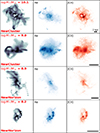 |
Fig. 1. Projection of the gas mass (left) and post-processed SKIRT output of the Hα (middle) and [C II] (right) emission of the most and least massive NEWCLUSTER (top two rows) and NEWHORIZON (bottom two rows) galaxies in a face-on configuration. The bar shows the physical scale of each source in kiloparsec. |
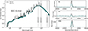 |
Fig. 2. Integrated spectral energy distribution of one representative NEWCLUSTER galaxy as produced by the SKIRT radiative transfer simulations assuming a DTM ratio of 16%. Left: Full SED in the observed frame, shown for the face-on (black) and edge-on (teal) configurations, spanning wavelengths from the ultraviolet to the millimeter. The shaded vertical regions show the coverage of ALMA bands 3, 7, and 9, and the dashed line demonstrates the JWST IFU range. Right: Examples of continuum-subtracted emission lines extracted from the same SED. |
3.2. Luminosities and SFR conversions
From the SEDs produced by SKIRT, we used the line-free continuum5 emission in the IR range between rest frames 8 and 1000 μm to estimate the total IR luminosity. We also estimated the line luminosities for Hα, Hβ, and [C II] at 158 μm at different inclinations using the continuum-free fluxes. In SKIRT, we adopted spectral resolutions that mimic those of JWST-IFU and ALMA, where the spectral lines are resolved with spectral channel widths of ∼ 100 km s−1 for Hα and Hβ, and ∼ 30 km s−1 for the [C II] line (see Sect. 3.1). We performed an automatic fitting procedure using the curve_fit function from Scipy, modeling each spectral line with a single Gaussian to estimate its flux (and luminosity) at each inclination. Because this routine returns a fit regardless of whether an emission line is present, we applied a signal-to-noise ratio (S/N) > 5 threshold to identify reliable detections. The S/N is defined as the ratio of the maximum line flux and the noise level, where the noise is estimated using the median absolute deviation of the spectrum excluding the emission line, measured over the velocity range 2500 and 4000 km s−1.
We finally converted luminosities into SFRs. Starting with Hα, one of the most widely used conversions between its luminosity (LHα) and SFR was derived by Kennicutt (1983) and calibrated for a Chabrier (2003) IMF by Murphy et al. (2011),
![Mathematical equation: $$ \begin{aligned} \mathrm {SFR}_{\rm {H}\alpha } \, [\mathrm {M}_\odot \mathrm {yr}^{-1}] = 5.37 \times 10^{-42} \, \textit{L}_{\rm {H}\alpha } \, [\mathrm {erg \, s}^{-1}], \end{aligned} $$](/articles/aa/full_html/2026/06/aa58893-26/aa58893-26-eq3.gif) (2)
(2)
where LHα is the attenuation-corrected luminosity. More recently, Reddy et al. (2022) derived a conversion factor for high-z galaxies based on the BPASS population synthesis models with lower stellar metallicities (Z* = 0.001) that includes stellar binaries assuming a Chabrier (2003) IMF with a maximum mass of 100 M⊙,
![Mathematical equation: $$ \begin{aligned} \mathrm {SFR}_{\rm {H}\alpha } \, [\mathrm {M}_\odot \mathrm {yr}^{-1}] = 2.14 \times 10^{-42} \, \textit{L}_{\rm {H}\alpha } \, [\mathrm {erg \, s}^{-1}]. \end{aligned} $$](/articles/aa/full_html/2026/06/aa58893-26/aa58893-26-eq4.gif) (3)
(3)
To correct for attenuation, we used the relation between the intrinsic (Fλ,int) and observed (Fλ,obs) fluxes that is given in the form
 (4)
(4)
where A(λ) = k(λ) E(B − V) is the attenuation at λ, k(λ) is the attenuation curve value at λ, and E(B − V) is the color excess between the B and V bands. In this case, the Balmer decrement was used to estimate the attenuation by comparing the observed line ratio of Hα to Hβ with the theoretical one. The Hα attenuation, AHα, can be summarized as follows:
 (5)
(5)
where (FHα/FHβ)obs and (FHα/FHβ)int are the observed (attenuated) and intrinsic (dust-free) line ratios, respectively. We used the intrinsic ratio of 2.86, assuming case B recombination with electron temperature T = 104 K and electron density ne = 100 cm−3 (Osterbrock & Ferland 2006). kHα = 2.53 and kHβ = 3.61 represent the attenuation curves at the Hα and Hβ wavelengths, respectively, adopting the Calzetti et al. (2000) attenuation law for local starbursts.
In addition to the attenuation correction applied to the observed Hα flux, this line is contaminated by the [N II] doublet at rest-frame wavelengths 6548 and 6583 Å. Several studies have investigated the effect of [N II] emission on the total flux of Hα, particularly its evolution with redshift (e.g., Kewley et al. 2013; Shapley et al. 2015; Kashino et al. 2017). Recent works suggested that the contribution from [N II] becomes negligible at z ≳ 4 (e.g., Sanders et al. 2023; Cameron et al. 2023) due to subsolar metallicities, but other studies indicated that a small correction might be necessary, with 96% of the total flux dominated by Hα (Sandles et al. 2024). We adopted the latter.
The IR luminosity is most commonly converted into SFR using the Kennicutt (1998) conversion modified for a Chabrier (2003) IMF,
![Mathematical equation: $$ \begin{aligned} \mathrm {SFR}_{\rm {IR}} \, [\mathrm {M}_\odot \mathrm {yr}^{-1}] = 1.09 \times 10^{-10} \, \textit{L}_{\rm {IR}} \, [\textit{L}_\odot ], \end{aligned} $$](/articles/aa/full_html/2026/06/aa58893-26/aa58893-26-eq7.gif) (6)
(6)
where LIR is the total IR luminosity integrated between rest frames 8 and 1000 μm. While this conversion is not the most recent, it remains widely used for high-z galaxies. At these redshifts, observational constraints typically provide access to only sparse continuum measurements (e.g., ALPINE-[C II] survey; Le Fèvre et al. 2020; Fudamoto et al. 2020). We computed LIR using the full IR continuum emission from the SKIRT outputs, however, which represents an idealized scenario in which the dust emission is fully sampled. In Sect. 5.4 we discuss the implications for real observations and whether measuring the peak of dust emission at these redshifts (e.g., with ALMA Band 9) would be sufficient.
Studies have also defined the total SFR, which is the addition of the IR and far-UV SFRs (e.g., Béthermin et al. 2020; Schaerer et al. 2020). This hybrid approach mitigates the dust attenuation that biases UV-based SFRs and missed IR contributions from less obscured regions. The total SFR is defined as
![Mathematical equation: $$ \begin{aligned} \mathrm {SFR}_{\rm {IR + UV}} \, [\mathrm {M}_\odot \, \mathrm {yr}^{-1}] = \mathrm {SFR}_{\rm {IR}} + \mathrm {SFR}_{\rm {UV}}, \end{aligned} $$](/articles/aa/full_html/2026/06/aa58893-26/aa58893-26-eq8.gif) (7)
(7)
where SFRIR = κIR LIR is the total IR-inferred SFR as defined in Eq. (6). SFRUV = κUV LUV, where LUV is the monochromatic luminosity at 1500 Å, and  is the conversion factor from luminosity to SFR assuming a Charbier IMF (Madau & Dickinson 2014). We note that we did not pursue a purely UV-based SFR analysis because its interpretation is strongly affected by dust attenuation, whose effect has been extensively studied (see Madau & Dickinson 2014, and references therein) and remains challenging to constrain.
Numerous studies have also explored the relation between the [C II] luminosity, L[C II], and the SFR as it probes the cooling of neutral and ionized gas heated by young starts (e.g., Stacey et al. 2010; De Looze et al. 2014; Herrera-Camus et al. 2015; Olsen et al. 2017; Lagache et al. 2018; Harikane et al. 2020; Schaerer et al. 2020; Accard et al. 2025). The relation can be expressed by a power law,
![Mathematical equation: $$ \begin{aligned} \log \, (L_{[\mathrm {C}{\small { {\text{ II}}}} ]}/L_\odot ) = \alpha + \gamma \, \log \, (\mathrm {SFR}/M_\odot \mathrm {yr}^{-1}), \end{aligned} $$](/articles/aa/full_html/2026/06/aa58893-26/aa58893-26-eq10.gif) (8)
(8)
where α and γ are calibration coefficients that depend on the considered samples. De Looze et al. (2014) investigated the reliability of the [C II] line as a SFR tracer using a diverse sample of galaxies with various types. They found a wide range of calibration coefficients between metal-poor dwarf galaxies, local starbursts, ultraluminous infrared galaxies, and high-redshift galaxies. Lagache et al. (2018) extended this analysis to 4 < z < 8 using semi-analytical simulations coupled with the photoionization code CLOUDY, while assuming that the [C II] line originates only from PDRs. They found a relation similar to that found in De Looze et al. (2014) for starburst galaxies and reported a small evolution of the L[C II] − SFR relation with redshift for L[C II] > 107 L⊙. We calibrated the coefficients to our sample and discuss this in Sect. 4.4.
4. Inferred SFRs
In this section, we derive the SFRs of each tracer, Hα in Sect. 4.1, the IR continuum in Sect. 4.2, and hybrid (IR + UV) in Sect. 4.3, and compare them to SFRtrue, that is, to the time-averaged SFR estimated from the simulation over 10 or 100 Myr. We note that when estimating SFRtrue, we corrected stellar particle masses with ages > 5 Myr for mass loss due to mass ejection during feedback processes: 31% in NEWHORIZON and 40% in NEWCLUSTER. For each of the three tracers, we performed a power law, finding the slope and offset based on the adopted conversions in Sect. 3.2. In Sect. 4.4 we calibrate the L[C II] − SFR coefficients to our sample of galaxies. The scatter of each tracer is estimated as the standard deviation of the residuals = log(SFRtracer/SFRtrue).
4.1. Hα SFR
In Fig. 3 the Balmer-corrected Hα SFRs as a function of SFR10 Myr are shown for a face-on configuration of NEWHORIZON- and NEWCLUSTER-simulated galaxies. A power-law fit to the simulation data using the Reddy et al. (2022) conversion (Eq. (3)) yields a slope of (0.83 ± 0.05) and an insignificant offset of 0.005 dex. This means that we overestimate SFRs with intrinsic SFR10 Myr below 5 M⊙ yr−1 and overestimate higher values up to a factor of ∼1.5. In contrast, the Murphy et al. (2011) conversion (Eq. (2)) yields the same slope, but the SFRs are systematically overestimated, for instance, SFR10 Myr < 300 M⊙ yr−1 with an offset of 0.4 dex. Based on these results, we adopted the Reddy et al. (2022) conversion for the rest of the study, for which we found a scatter of 0.37 dex.
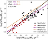 |
Fig. 3. Hα-derived SFRs using Eq. (3) vs. SFR10 Myr for NEWCLUSTER (black squares) and NEWHORIZON (red circles) simulated galaxies in a face-on configuration. The identity line is shown in black, and the dotted purple and orange lines show the best-fit of the Hα-derived SFRs using the conversion of Reddy et al. (2022) and Murphy et al. (2011), respectively (see Sect. 4.1 for details). In the top left corner, the slopes and offsets are shown with the same color code as the lines, and the scatter σ of the inferred SFRs. |
In Fig. 4 we inspect the effect of inclination on the derived SFRs since geometrical configurations have a direct effect on attenuation, especially at shorter wavelengths. For an edge-on configuration, we found that the inferred SFRs reproduce SFR10 Myr similar to the face-on configuration with a slope of (0.83 ± 0.06) and a small offset of −0.02 dex. However, we find an increase in scatter up to 0.41 dex that is due to an increase in the column densities along the line of sight. The scatter varies between different inclinations and reaches ∼0.5 dex for an inclination of 60° (see Fig. B.1 for the effect of different inclinations). We note that Hα is detected in most sources across inclinations, while Hβ detections vary across inclinations, thus varying the number of sources for which we estimated a SFR, and might slightly vary the scatter.
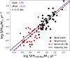 |
Fig. 5. Same as Fig. 3 for the IR-inferred SFRs vs. time-averaged SFR over 100 Myr. The SFRs are derived using Kennicutt (1998) conversion (Eq. (6)), and the best fit is shown by the dashed purple line. |
A clear difference is observed between the two simulations: NEWHORIZON sources exhibit a lower scatter of ∼0.2 dex, while NEWCLUSTER sources show a broader distribution with a scatter of ∼0.5 dex and a small number of outliers. This trend continues to hold at different inclinations (see Fig. 4 and B.1). We inspected the line profiles and spectral fits of the NEWCLUSTER sources that contribute to the larger scatter (i.e., those with residuals > 0.7 dex) and found no failure originating in the method of the spectral fitting. These differences can have several reasons. NEWCLUSTER galaxies are generally more massive and have higher gas masses than NEWHORIZON ones, which leads to higher dust masses at a fixed DTM (see Eq. (1)) and higher dust optical depths. The comparison of lower-mass NEWCLUSTER galaxies with NEWHORIZON counterparts reveals similar behavior, suggesting that the scatter is primarily driven by underlying physical processes and not by simulation-specific conditions.
While a single attenuation curve has shown to produce adequate results for z = 5 galaxies from the low- to the high-mass end on average, increased dust optical depths, dust distributions, and dust geometry make attenuation curves nontrivial (e.g., Scicluna & Siebenmorgen 2015; Lin et al. 2021). This highlights that optical tracers at these redshifts are highly susceptible to uncertainties introduced by complex dust physics, particularly for high-mass systems. We further explore the attenuation curves in Sect. 5.2.
4.2. IR SFR
The inferred SFRs from the total IR luminosity using the Kennicutt (1998) conversion reproduce the SFRs traced by the simulations over 100 Myr timescales with a slope close to unity (1.09 ± 0.06) and an offset of −0.19 dex. In contrast to SFRHα, we systematically underestimate SFR100 Myr below ∼ 30 − 50 M⊙ yr−1 and overestimate higher SFRs by a factor of ∼1.5.
We found a scatter of 0.37 dex whose origin is generally due to differences in stochastic heating of small dust grains (Draine & Li 2001). As expected, we do not see variations in the resulting SFRs (and a constant dispersion) when we changed the galaxy inclinations (Fig. B.1). However, we can see a difference in the scatter between NEWHORIZON (0.41 dex) and NEWCLUSTER galaxies (0.28 dex), which could be attributed to several factors, such as galaxy mass, star formation histories (SFH), and dust content.
As mentioned in Sect. 4.1, NEWHORIZON galaxies have a lower dust content than NEWCLUSTER ones. Systems with lower dust masses tend to have a higher leakage of UV photons and thus lower IR luminosities (Buat et al. 2007), where it is argued that SFRs become questionable when LIR < 109.5 L⊙ (Rieke et al. 2009). We estimated the monochromatic far-UV luminosities for a face-on configuration using the rest-frame 1500 Å flux densities and inferred the IR-to-UV ratio. We found that this ratio varies homogeneously in both samples (see Fig. C.1), which explains some of the increased scatter observed for NEWHORIZON galaxies. We discuss this further in Sect. 4.3.
Studies have also shown that low-mass galaxies (at M* < 108.5 M⊙) experience a more stochastic, bursty star formation than their higher-mass counterparts (e.g., Ciesla et al. 2024; Perry et al. 2025; Covelo-Paz et al. 2025). The NEWHORIZON and NEWCLUSTER simulations both capture this bursty star formation (see details in Dubois et al. 2021; Han et al. 2026). The SFH of our galaxies shows evidence of bursty star formation over timescales of ∼10 Myr (see Appendix D and Fig. D.1). This means that while the IR conversion to SFR offers a good estimate of SFRs time-averaged over 100 Myr, it fails to do so when galaxies undergo bursty episodes of star formation, leading to increased uncertainties, particularly for low-mass NEWHORIZON galaxies (M* < 109 M⊙). This agrees with the literature.
4.3. Hybrid SFR (IR + UV)
Figure 6 shows the hybrid SFR estimated using Eq. (7) versus SFR100 Myr for our sources. We find a slope very close to unity (0.93 ± 0.04) and an offset of 0.1 dex. As expected from the previous discussion on SFRIR, the dispersion significantly decreases to 0.27 dex.
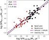 |
Fig. 6. Same as Fig. 3 for the hybrid-inferred SFRs (IR + UV) vs. time-averaged SFR over 100 Myr. The SFRs are derived using the conversion in Eq. (7), and the best fit is shown by the dashed purple line. |
The scatter significantly decreases for the less massive NEWHORIZON sources, dropping from 0.41 dex for IR-inferred SFRs (see Fig. 5) to 0.3 dex, but only a slight decrease in scatter is observed for NEWCLUSTER sources (from 0.28 to 0.25 dex). The lower gas content (∝ dust content) in these systems leads to significant UV photon leakage (see Fig. C.1), which makes the IR luminosity an incomplete tracer of the total star formation. By accounting for the unattenuated UV component, the hybrid tracer recovers the escaped radiation, providing a more robust SFR time-averaged over 100 Myr particularly for the low-mass regimes (M* < 109 M⊙). Additionally, the offset decreases from 0.1 to 0.06 dex when the galaxies are rotated to an edge-on configuration (Fig. B.1). This improvement is likely due to the increased optical depth along the line of sight, which decreases the sensitivity to UV luminosity variations that may contribute to the observed offset.
Despite these improvements, a scatter of 0.27 dex remains. This suggests that while the hybrid SFR corrects for underestimated IR luminosities due to UV-photon leakage, it cannot eliminate uncertainties arising from SFH stochasticity and the stochastic heating of small dust grains, both of which contribute to the scatter of IR luminosities.
4.4. [C II] SFR
In Fig. 7 we plot L[C II] as a function of SFR100 Myr. We performed a linear regression fit to our sample of simulated sources, deriving the following relation:
![Mathematical equation: $$ \begin{aligned} \log \, (L_{[\mathrm C{\small { {\text{ II}}}}\mathrm ]}/L_\odot ) = (6.06 \pm 0.09) + (1.39 \pm 0.10) \log \, \mathrm {(SFR/M_\odot yr^{-1})}. \end{aligned} $$](/articles/aa/full_html/2026/06/aa58893-26/aa58893-26-eq11.gif) (9)
(9)
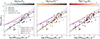 |
Fig. 7. [C II] luminosity as a function of SFR100 Myr of NEWHORIZON- and NEWCLUSTER-simulated sources shown as circles and squares, respectively. The data points are color-coded based on the median of gas metallicities (left), the median of gas densities (middle), and the peak temperature (right) in a given source (see Sect. 4.4 for details). The dash-dotted black line shows the L[C II] − SFR relation we obtained. The dash-dotted purple, dotted blue, red, dashed green, and dashed magenta lines represent L[C II] − SFR relations by Olsen et al. (2017, z = 6), Lagache et al. (2018, z = 5), Schaerer et al. (2020, 4 < z < 6), Harikane et al. (2020, 6 < z < 9), and Accard et al. (2025, 4 < z < 6), respectively. |
The slope we found is generally steeper than most values derived in the literature. Schaerer et al. (2020) derived the relation for massive (M* > 1010 M⊙) z ∼ 5 ALMA-observed sources from the ALPINE (Le Fèvre et al. 2020; Fudamoto et al. 2020) sample of galaxies, finding a slope close to unity (0.96 ± 0.09). Our values are closer to the findings of Accard et al. (2025), however, where the reported slope was ∼1.25 ± 0.25 using resolved measurements of ALMA-observed galaxies at z ∼ 5. Harikane et al. (2020) find an even steeper slope = 1.6 for a sample of z = 6 − 9 ALMA-observed galaxies. Lagache et al. (2018) derive a relation that varied with redshift, where the slope = 1.05 at z = 5 for a sample of semi-analytical simulated galaxies with L[C II] > 107 L⊙. Interestingly, some of our sources, particularly at similar L[C II], lie on the relation found in Lagache et al. (2018). Olsen et al. (2017) found a significantly shallower slope of 0.58 ± 0.11 at z = 6 for a sample of 30 main-sequence galaxies from the MUFASA cosmological simulation (Davé et al. 2016), post-processed with CLOUDY. Their inferred [C II] luminosities are generally fainter (6 × 10⁶ < L[C II] < 6 × 10⁷ L⊙) than those in Lagache et al. (2018). By limiting our sample to the respective luminosities of the mentioned samples, we found slopes of 0.99 ± 0.18 and 0.37 ± 0.09 – both of which agree with Lagache et al. (2018) and Olsen et al. (2017). This highlights that the slope of the L[C II] − SFR relation may depend on the luminosity range probed.
The inferred SFRs show a uniform behavior in both samples. We found that they reproduce SFR100 Myr with a scatter of 0.35 dex at all inclinations (see Fig. B.1). Because [C II] is generally optically thin and is unaffected by dust attenuation, we expect no significant variations in the integrated luminosities or the corresponding inferred SFRs. De Looze et al. (2014) demonstrated that while a correlation exists between the [C II] emission and SFR, this relation is dispersed, where they found a scatter of ∼0.41 dex for observed galaxies. Recent results of the resolved [C II] – SFR relation (Accard et al. 2025) of ALMA-observed galaxies at z ∼ 5 show a smaller intrinsic of 0.19 dex, suggesting that properly accounting for measurements and their uncertainties can significantly decrease the scatter. It was also shown that the relation is highly dependent on gas density, metallicity, and dust temperature (see also Herrera-Camus et al. 2015; Liang et al. 2024).
While our data are unaffected by observational uncertainties, we further studied the dependence of this correlation on the physical parameters of the ISM. In SKIRT, the [C II] line is produced using the TODDLERS template for star-forming regions. To this end, we computed for each galaxy the median gas density and the median metallicity of star-forming regions with stellar ages < 10 Myr (see Sect. 3.1 for our detailed configuration in SKIRT). In the left and middle panels, we show the L[C II] − SFR color-coded by the gas metallicity and density, respectively. Galaxies with a lower metallicity clearly lie above the relation and galaxies with a higher metallicity lie below it, while the gas density shows the opposite of the trend found for the metallicity.
We also assessed the dependence on the dust temperature (right panel). For simplicity, we estimated the dust temperature by assuming Wien’s law6 (λpeak T = 2.989 × 103 μm K). However, most of the peak source temperatures are ∼33 K, making the sample relatively homogeneous. Only a few sources have higher temperatures, reaching ∼40 K, and over this limited 10 K range, a temperature dependence is not evident.
5. Discussion
5.1. Effect of the DTM ratio on SFRs
The DTM has been studied in depth, particularly in the local Universe (e.g., Rémy-Ruyer et al. 2014; De Vis et al. 2019). At higher redshifts, studies suggest that the DTM ratio depends on the gas metallicity (e.g., Li et al. 2019) and redshift (e.g., Inoue 2003). Popping et al. (2017) found a varying DTM with gas metallicity, stellar mass, and redshift, with DTM < 18% at z = 5 for all metallicities and stellar masses, which is consistent with the relation of Vogelsberger et al. (2020). A ratio similar to the Galactic one was also adopted throughout the literature (∼40% Liang et al. 2019). In this section, we explore higher DTM ratios, particularly 25% and 40% (in addition to the previously adopted value of 16%), to understand its effect on the inferred SFRs. The results are shown in Fig. 8 for all four tracers.
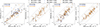 |
Fig. 8. Effect of DTEM on SFR estimates of Hα vs. SFR10 Myr, [C II] at 158 μm vs. SFR100 Myr, IR vs. SFR100 Myr, and gybrid (UV+IR) vs. SFR100 Myr (left to right) for NEWCLUSTER (squares) and NEWHORIZON (circles) simulated galaxies. The DTM ratios considered are 16% (black), 25% (blue), and 40% (orange). The solid gray line is the identity line, and the dashed, dotted, and dash-dotted lines indicate offsets of ±0.3, ±0.7, and ±1 dex, respectively. In the top left corner of each plot, the dispersion of the entire sample is shown. |
As expected, the scatter for the Hα-derived SFRs increases substantially (from 0.37 to 0.5 dex). At these wavelengths, the attenuation strongly affects the ability to recover the intrinsic SFRs, and as previously stated, larger dust reservoirs (i.e., higher optical depths for a fixed galaxy size) introduce more scatter due to the complexity of attenuation curves (e.g., Scicluna & Siebenmorgen 2015; Lin et al. 2021). Additionally, the total sample decreases due to Hβ nondetections for DTM = 40% with a total of 71 sources, compared to 85 sources for a DTM of 16%, further increasing the scatter. In contrast, [C II], IR continuum, and hybrid (UV+IR) SFRs show little to no variation when the DTM changed. Nevertheless, we found a modest increase in the IR-inferred SFRs, by a factor of 1.13, when we adopted a DTM of 40%. This trend reflects the higher dust masses at higher DTM values, which enhance the far-IR peak of the SED and thus increase the total IR luminosities. In addition, the scatter in the IR-inferred SFRs decreases slightly, from 0.37 to 0.35 dex, which is driven by the increased dust column densities that limit the leakage of UV photons.
For the remainder of the study, we adopt DTM = 16% unless stated otherwise.
5.2. Hα attenuation
The Hα-derived SFRs are strongly dependent on the assumed attenuation law. While the Calzetti et al. (2000) laws have been widely used for high-z studies, particularly the calibrations made for local starbursts, we are still limited in our understanding of the ISM at these redshifts. We explored the attenuation curve for our simulated sources from the NEWHORIZON and NEWCLUSTER simulations.
Using the TODDLERS library, we processed the sources with SKIRT while excluding dust (includeDust="false") following the same criteria as outlined in Sect. 3.1. This allowed us to recover the intrinsic Hα line flux. Combined with the attenuated line fluxes, we estimated the Hα attenuation AHα = −2.5log(Fobs/Fint). We also estimated the ratio of Hα and Hβ attenuation curves, kHα/kHβ, using Eq. (5). In Fig. 9 we show the derived attenuation curve ratios for a varying DTM compared to some of the attenuation laws in the literature.
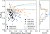 |
Fig. 9. Left: Ratio of the Hα and Hβ attenuation laws derived vs. the Hα attenuation for NEWHORIZON (circles) and NEWCLUSTER (squares) simulated galaxies. Black, blue, and orange represent DTM ratios of 16%, 25%, and 40%, respectively. The ratio derived for simulated galaxies from Tacchella et al. (2022) (dashed gray line) and Kapoor et al. (2024) (dash-dotted teal line) and that derived by Calzetti et al. (2000) (dashed blue line) for local starbursts are shown. Right: Distribution of the derived attenuation law ratios for our sources at different DTM ratios. |
We found that our sources exhibit a large scatter and systematically lie below the relations derived by Tacchella et al. (2022) and Kapoor et al. (2024) for local simulated sources and post-processed with SKIRT. We note that their curves were derived from spatially resolved maps, which we did not pursue. As expected, the attenuation (AHα) increases with DTM. For the NEWHORIZON and NEWCLUSTER sources, the resulting kHα/kHβ ratios span broad ranges: for DTM = 16%, the values range from ∼0.4 − 0.7, for DTM = 25%, they range from ∼0.5 − 0.7, and for DTM = 40%, they range from ∼0.55 − 0.72 (see the histogram in Fig. 9). These values agree in general with earlier high-redshift studies (z < 3; e.g., Buat et al. 2012; Kriek & Conroy 2013; Reddy et al. 2015) and more recent ones with JWST (Cooper et al. 2025), who argued that attenuation curves are steeper (i.e., lower kHα/kHβ values) at these redshifts than the widely used curve with a ratio ∼0.7 found by Calzetti et al. (2000) for local starbursts. Additionally, the attenuation curves flatten with DTM, as expected because the optical depth increases (Narayanan et al. 2018). Sources from both simulations exhibit differences in the attenuation curve, where NEWHORIZON galaxies exhibit shallower curves (i.e., higher kHα/kHβ values) and vice versa, which are attributed to their physical conditions (e.g., Shivaei et al. 2020, 2026). By using an average value of the attenuation curve ratio of 0.58, we reestimated the Hα-corrected SFRs (see Fig. E.1) and found a significant decrease in the scatter that reached 0.16 dex at SFR < 5 M⊙ yr−1, but underestimated the SFR by a factor of ∼2 at higher SFRs. These results highlight the importance of obtaining a more diverse library of attenuation curves that can constrain the corrections applied to the attenuation at high z better.
5.3. [C II] deficit
In the local Universe, the [C II] deficit is defined as a systematic decrease in the L[C II]/LIR ratio with increasing LIR, observed for luminous and ultra-luminous infrared galaxies (e.g., Muñoz & Oh 2016; Díaz-Santos et al. 2017). In contrast, at highz, it is used to describe galaxies with L[C II]/LIR < 10−3 for IR-bright sources (≳1012 L⊙), even in the absence of a decreasing trend. This deficit is attributed to different factors, such as increased dust column densities, reduced photoelectric heating, or [C II] saturation at a high gas temperature (e.g., Casey et al. 2014; Goicoechea et al. 2015; Muñoz & Oh 2016).
In Fig. 10 we plot the L[C II]/LIR ratio estimated for the NEWHORIZON- and NEWCLUSTER-simulated galaxies as a function of the IR luminosity. The L[C II]/LIR ratio varies between ∼10−4 and ∼2 × 10⁻³ for the entire sample. Within the luminosity ranges we considered, particularly within the 1011 − 1012 L⊙ range, the ratio is comparable to that of z ∼ 5 sources. For comparison, we plot the ALPINE-[C II] survey sources (Schaerer et al. 2020), which align with the most luminous NEWCLUSTER sources, even though they occupy a narrow range in the L[C II]/LIR − SFR LIR space. While ALPINE sources are more massive than NEWCLUSTER galaxies, we were able to reproduce the observed ratios of bright [C II] emitters on average. In general, we found that galaxies from both simulations display an increasing trend in the L[C II]/LIR − SFR LIR plane. However, some sources deviate from the general trend and show exceptionally low ratios. To explore the deviation from the general trend, we investigated the ratio dependence on gas metallicity and gas density, represented by color maps in Fig. 10. In the left panel, a clear deviation is observed for some sources with increased metallicities, where the L[C II]/LIR ratio decreases with increasing LIR, particularly for the NEWCLUSTER sources. In the right panel, the gas density shows a similar trend, where a [C II] deficit appears to follow sources with a lower gas density. At this stage, it is difficult to draw conclusions from a few data points. As reported previously, we found no difference in the [C II] luminosities and a modest increase of 13% in IR luminosities while varying the DTM ratios, which means that increased dust column densities would not affect the [C II]-IR luminosity ratios of our sample significantly.
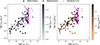 |
Fig. 10. [C II]/IR luminosity ratios vs. IR luminosity of NEWCLUSTER (squares) and NEWHORIZON (circles). We color-code our sources based on the median gas metallicity (left) and median gas density (right) of each galaxy. We plot the observed ALPINE z ∼ 4 − 6 sources in purple (Schaerer et al. 2020) for comparison. |
5.4. LIR with realistic IR sampling
In Sect. 4.2 we presented an ideal-case scenario of estimating LIR assuming that we are able to sample the IR SED between rest frames 8 and 1000 μm. However, this is not a realistic coverage for high-z galaxies, whose current sampling is limited to a few measurements in the far-IR with instruments like ALMA and, when available, mid-IR from JWST-MIRI. Particularly, some of the [C II] surveys at z > 4 are limited to one photometric measurement in the IR, which has motivated approaches based on stacking (e.g., Béthermin et al. 2020) or deriving dust temperatures from a single continuum measurement combined with priors or scaling relations (Sommovigo et al. 2022). Béthermin et al. (2020) also derived the ratio of monochromatic continuum luminosity to the total IR luminosity. We investigated two approaches: 1) luminosities inferred from a modified blackbody, and 2) monochromatic luminosities (νLν) at a rest-frame frequency ν.
To understand whether a modified blackbody (MBB) might estimate a reliable LIR, we assumed that we are able to sample the peak of dust emission in addition to the photometric data from ALMA band 7, where the [C II] line is observed. For galaxies at z = 5, the peak of dust emission is roughly in the observed wavelength range λ ∼ 0.4 − 0.5 mm, which is covered by ALMA Band 9. From SKIRT, we obtained the broadband fluxes7 of ALMA bands 7 and 9 with central wavelengths at 450 and 940 μm, respectively (see Fig. 2). The data were fit with a single-temperature MBB in its optically thin form and sampled using EMCEE (Foreman-Mackey et al. 2013). We followed the method described in Ismail et al. (2023), which also accounts for the CMB effects (da Cunha et al. 2013), but we fixed the value of the dust emissivity index to β = 2.2 following the findings in Ismail et al. (2023), Algera et al. (2025), Boogaard et al. (2026). In the case of monochromatic luminosities, we estimated νLν for ALMA bands 7 and 9, which correspond to rest-frame wavelengths  m and
m and  m at z = 5, respectively.
In Fig. 11 we compare IR luminosities inferred from the different approaches to the total LIR derived from a fully sampled continuum in Sect. 4.2. We also fit a power law to assess the relation between them. We found that all three cases, the MBB and the monochromatic luminosities, systematically underestimate the total IR luminosity, but the resulting slopes are ∼1. The MBB fit underestimates the total luminosity by a factor of ∼2 (−0.29 ± 0.06 dex). This is expected since the MBB models the far-IR emission of large thermal dust grains, but fails to capture the contribution from small grains and polycyclic aromatic hydrocarbons at wavelengths λrest < 50 μm. Interestingly, the monochromatic luminosity at ALMA band 9 performs similarly to the MBB with an offset of −0.27 ± 0.08 dex. This arises because band 9 closely samples the peak of the dust SED of our sample. Because our galaxies exhibit a relatively uniform peak dust temperature of ∼33 K (see Sect. 4.4), the monochromatic measurement at rest-frame 75 μm captures the bulk of the energy emission with little scatter, which would not be the case if the dust temperature varied. The monochromatic luminosity in band 7, on the other hand, underestimates the total LIR by a factor of ∼4.4 (0.64 ± 0.19 dex), which is smaller than the factor found in Béthermin et al. (2020, ∼6.5), but their SEDs exhibit dust temperatures > 40 K. While the correlation stays tight following a nearly linear slope (0.98 ± 0.02), the scatter is larger since the emission is sensitive to the dust mass and dust grain properties at these wavelengths, assuming a constant dust temperature. Nevertheless, the linearity of these relations provide a framework based on which we can correct for the total LIR for z = 5 galaxy samples, where current observations are limited in photometric measurements.
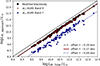 |
Fig. 11. Infrared luminosities derived using different approaches vs. the IR luminosity derived in Sect. 6 for our entire sample. The black squares show LIR derived using a modified blackbody, the red circles show LIR derived from the monochromatic luminosity from ALMA band 9, and blue stars show those derived from the monochromatic luminosity from ALMA band 7. The black line is the identity line, and the dashed black, solid red, and dotted blue lines represent the best fit of each inferred LIR. |
6. Summary and conclusions
We analyzed simulated galaxies at z = 5 drawn from two hydrodynamical cosmological zoom-in simulations, NEWHORIZON and NEWCLUSTER, which were post-processed with the 3D radiative transfer code SKIRT. We derived SFRs using observables relevant at high z: the Hα nebular emission line, the [C II] 158 μm fine-structure line, and the FUV and IR continua. These observables were generated at spectral resolutions comparable to those of current facilities, namely JWST and ALMA. We further examined how the inferred SFRs depend on the physical properties of the interstellar medium and on intrinsic factors such as the viewing angle and the dust-to-metal ratio. Our main findings are summarized below.
-
The Hα–inferred SFRs, corrected via the Balmer decrement, reproduce the intrinsic SFRs with timescales of 10 Myr using the Reddy et al. (2022) conversion, while it is overestimated with the Kennicutt (1983) conversion. Nevertheless, the inferred SFRs exhibit the largest dispersion of all tracers, with a scatter that varies between 0.3 to 0.5 dex for the entire sample because it depends on the viewing angle and the assumed dust-to-metal ratio. For more massive sources (M* > 109 M⊙), the scatter is significantly larger (∼0.5 dex) than for the lower-mass galaxies (∼0.2 dex), primarily because their dust reservoirs are larger and their dust optical depths are correspondingly higher, which increases the complexity of attenuation corrections. We inferred an effective attenuation ratio of kHα/kHβ spanning 0.4 − 0.7 across different dust-to-metal ratio assumptions, which is generally steeper than the canonical ratio of 0.7 that is usually assumed. A value of 0.58 reduces the scatter at low SFRs, but leads to an underestimation of the inferred SFRs by a factor of ∼2 at high intrinsic SFRs.
-
The IR-inferred SFRs reproduce intrinsic SFRs time-averaged over 100 Myr with a slope close to unity and a small offset of −0.19 that underestimates intrinsically low SFRs. These SFRs exhibit a significant scatter of 0.37 dex that is due to bursty SFHs and to UV-photon leakage, which becomes significant in galaxies with a lower gas content. Under a realistic sampling of the IR energy distribution, we derived correction factors to recover the IR luminosities from limited data. We found that LIR is underestimated by a factor of ∼2 for a MBB and monochromatic luminosities at the peak of the SED (ALMA band 9 in this case). Measurements along the RJ tail with ALMA band 7 exhibit a larger underestimation by a factor of ∼4.4.
-
The hybrid SFR (UV + IR) shows a lower scatter of 0.27 dex than IR-based SFRs. The inferred SFRs reproduce intrinsic SFRs over 100 Myr timescales, with a slope close to unity and a small offset of 0.1 dex. This hybrid estimator mitigates the effect of UV-photon leakage that contributes to the scatter in IR continuum-based SFRs while simultaneously avoiding the need for uncertain dust attenuation corrections to the UV emission. This makes it a robust SFR tracer for UV-selected samples, particularly for galaxies with a lower gas content.
-
The [C II]-inferred SFRs show a consistent but relatively high scatter of 0.36 dex around the identity line. We found the [C II] to be independent of the viewing angle and DTM ratio, making it more robust as a SFR tracer than the former optical line. The L[C II] − SFR relation for our sample of galaxies exhibits a steep slope of ∼1.4 and a high scatter. We demonstrated that the steepness of this relation is sensitive to the range of luminosities assumed for the fit, and the scatter depends on gas metallicity and gas density. This agrees with literature studies. We also showed that our most massive galaxies from NEWCLUSTER reproduce the L[C II]/LIR ratios of ALMA-observed sources from the ALPINE survey. A general increasing trend is observed between L[C II]/LIR and LIR, but a [C II] deficit is not very clear with the current galaxy sample.
In summary, we provided quantitative benchmarks for widely used observables at z = 5 across galaxies spanning a wide range of stellar masses (8 < log M*/M⊙ < 10). In the future, we will explore these tracers in more detail, particularly the emission lines, while also integrating nonuniform dust distribution and properties that are modeled on the fly in the NEWCLUSTER simulation.
Acknowledgments
We thank the anonymous referee for the insightful comments that helped improve the manuscript. S.K.Y. acknowledges support from the Korean National Research Foundation (RS-2025-00514475 and RS-2022-NR070872). This work was granted access to the HPC resources of KISTI under the allocations KSC-2021-CRE-0486, KSC-2022-CRE-0088, KSC-2022-CRE-0344, KSC-2022-CRE-0409, KSC-2023-CRE-0343, KSC-2024-CHA-0009, and KSC-2025-CRE-0031 and of GENCI under the allocation A0150414625 and A0180416216. The large data transfer was supported by KREONET which is managed and operated by KISTI. This work was granted access to the HPC resources of CINES under the allocations c2016047637, A0020407637, and A0070402192 by Genci, KSC-2017-G2-0003, KSC-2020-CRE-0055, and KSC-2020-CRE-0280 by KISTI, and as a “Grand Challenge” project granted by GENCI on the AMD Rome extension of the Joliot Curie supercomputer at TGCC. D.I. is grateful to Alfred Gulum for his unwavering enthusiasm, even when the scatter was not. T.K. is supported by the National Research Foundation of Korea (RS-2022-NR070872 and RS-2025-00516961) and the Yonsei Fellowship, funded by Lee Youn Jae. A.U.K. acknowledges support from the Belgian Federal Science Policy Office (BELSPO) via the ESA-PRODEX programme. C.A. acknowledges that this work of the Interdisciplinary Thematic Institute IRMIA++, as part of the ITI 2021-2028 program of the University of Strasbourg, CNRS and Inserm, was supported by IdEx Unistra (ANR-10-IDEX-0002), and by SFRI-STRAT’US project (ANR-20-SFRI-0012) under the framework of the French Investments for the Future Program.
References
- Accard, C., Béthermin, M., Boquien, M., et al. 2025, A&A, 702, A206 [NASA ADS] [CrossRef] [EDP Sciences] [Google Scholar]
- Algera, H. S. B., Herrera-Camus, R., Aravena, M., et al. 2025, A&A, submitted, [arXiv:2512.02320] [Google Scholar]
- Arun, R. 2025, AJ, 170, 196 [Google Scholar]
- Baes, M., & Camps, P. 2015, Astron. Comput., 12, 33 [NASA ADS] [CrossRef] [Google Scholar]
- Béthermin, M., Fudamoto, Y., Ginolfi, M., et al. 2020, A&A, 643, A2 [Google Scholar]
- Boogaard, L. A., Walter, F., Weiß, A., et al. 2026, ApJ, 996, 19 [Google Scholar]
- Bouwens, R. J., Illingworth, G. D., Franx, M., et al. 2009, ApJ, 705, 936 [Google Scholar]
- Bruzual, G., & Charlot, S. 2003, MNRAS, 344, 1000 [NASA ADS] [CrossRef] [Google Scholar]
- Buat, V., Takeuchi, T. T., Iglesias-Páramo, J., et al. 2007, ApJS, 173, 404 [Google Scholar]
- Buat, V., Noll, S., Burgarella, D., et al. 2012, A&A, 545, A141 [NASA ADS] [CrossRef] [EDP Sciences] [Google Scholar]
- Buat, V., Heinis, S., Boquien, M., et al. 2014, A&A, 561, A39 [NASA ADS] [CrossRef] [EDP Sciences] [Google Scholar]
- Byun, G.-H., Jang, J. K., Scofield, Z. P., et al. 2025, ApJ, 992, 92 [Google Scholar]
- Calzetti, D., Armus, L., Bohlin, R. C., et al. 2000, ApJ, 533, 682 [NASA ADS] [CrossRef] [Google Scholar]
- Cameron, A. J., Saxena, A., Bunker, A. J., et al. 2023, A&A, 677, A115 [NASA ADS] [CrossRef] [EDP Sciences] [Google Scholar]
- Camps, P., & Baes, M. 2020, Astron. Comput., 31, 100381 [NASA ADS] [CrossRef] [Google Scholar]
- Camps, P., Trčka, A., Trayford, J., et al. 2018, ApJS, 234, 20 [NASA ADS] [CrossRef] [Google Scholar]
- Casey, C. M., Narayanan, D., & Cooray, A. 2014, Phys. Rep., 541, 45 [Google Scholar]
- Chabrier, G. 2003, PASP, 115, 763 [Google Scholar]
- Ciesla, L., Elbaz, D., Ilbert, O., et al. 2024, A&A, 686, A128 [NASA ADS] [CrossRef] [EDP Sciences] [Google Scholar]
- Cooper, O. R., Brammer, G., Heintz, K. E., et al. 2025, ApJ, 982, 125 [Google Scholar]
- Covelo-Paz, A., Giovinazzo, E., Oesch, P. A., et al. 2025, A&A, 694, A178 [NASA ADS] [CrossRef] [EDP Sciences] [Google Scholar]
- da Cunha, E., Groves, B., Walter, F., et al. 2013, ApJ, 766, 13 [Google Scholar]
- Davé, R., Thompson, R., & Hopkins, P. F. 2016, MNRAS, 462, 3265 [Google Scholar]
- De Looze, I., Cormier, D., Lebouteiller, V., et al. 2014, A&A, 568, A62 [NASA ADS] [CrossRef] [EDP Sciences] [Google Scholar]
- De Vis, P., Jones, A., Viaene, S., et al. 2019, A&A, 623, A5 [NASA ADS] [CrossRef] [EDP Sciences] [Google Scholar]
- Díaz-Santos, T., Armus, L., Charmandaris, V., et al. 2017, ApJ, 846, 32 [Google Scholar]
- Draine, B. T., & Li, A. 2001, ApJ, 551, 807 [NASA ADS] [CrossRef] [Google Scholar]
- Draine, B. T., & Salpeter, E. E. 1979, ApJ, 231, 438 [Google Scholar]
- Dubois, Y., Devriendt, J., Slyz, A., & Teyssier, R. 2012, MNRAS, 420, 2662 [Google Scholar]
- Dubois, Y., Pichon, C., Welker, C., et al. 2014, MNRAS, 444, 1453 [Google Scholar]
- Dubois, Y., Beckmann, R., Bournaud, F., et al. 2021, A&A, 651, A109 [NASA ADS] [CrossRef] [EDP Sciences] [Google Scholar]
- Dubois, Y., Rodríguez Montero, F., Guerra, C., et al. 2024, A&A, 687, A240 [NASA ADS] [CrossRef] [EDP Sciences] [Google Scholar]
- Federrath, C., & Klessen, R. S. 2012, ApJ, 761, 156 [Google Scholar]
- Ferruit, P., Jakobsen, P., Giardino, G., et al. 2022, A&A, 661, A81 [NASA ADS] [CrossRef] [EDP Sciences] [Google Scholar]
- Figueira, M., Pollo, A., Małek, K., et al. 2022, A&A, 667, A29 [NASA ADS] [CrossRef] [EDP Sciences] [Google Scholar]
- Foreman-Mackey, D., Hogg, D. W., Lang, D., & Goodman, J. 2013, PASP, 125, 306 [Google Scholar]
- Freundlich, J., Combes, F., Tacconi, L. J., et al. 2019, A&A, 622, A105 [NASA ADS] [CrossRef] [EDP Sciences] [Google Scholar]
- Fudamoto, Y., Oesch, P. A., Faisst, A., et al. 2020, A&A, 643, A4 [NASA ADS] [CrossRef] [EDP Sciences] [Google Scholar]
- Goicoechea, J. R., Teyssier, D., Etxaluze, M., et al. 2015, ApJ, 812, 75 [Google Scholar]
- Groves, B., Brinchmann, J., & Walcher, C. J. 2012, MNRAS, 419, 1402 [NASA ADS] [CrossRef] [Google Scholar]
- Haardt, F., & Madau, P. 1996, ApJ, 461, 20 [Google Scholar]
- Han, S., Dubois, Y., Lee, J., et al. 2025, ApJ, 978, 96 [Google Scholar]
- Han, S., Yi, S. K., Dubois, Y., et al. 2026, A&A, 705, A169 [NASA ADS] [CrossRef] [EDP Sciences] [Google Scholar]
- Harikane, Y., Ouchi, M., Inoue, A. K., et al. 2020, ApJ, 896, 93 [Google Scholar]
- Herrera-Camus, R., Bolatto, A. D., Wolfire, M. G., et al. 2015, ApJ, 800, 1 [Google Scholar]
- Hirashita, H., Buat, V., & Inoue, A. K. 2003, A&A, 410, 83 [NASA ADS] [CrossRef] [EDP Sciences] [Google Scholar]
- Hirashita, H., Nozawa, T., Villaume, A., & Srinivasan, S. 2015, MNRAS, 454, 1620 [NASA ADS] [CrossRef] [Google Scholar]
- Inoue, A. K. 2003, PASJ, 55, 901 [NASA ADS] [CrossRef] [Google Scholar]
- Ismail, D., Beelen, A., Buat, V., et al. 2023, A&A, 678, A27 [Google Scholar]
- Iwamoto, K., Brachwitz, F., Nomoto, K., et al. 1999, ApJS, 125, 439 [NASA ADS] [CrossRef] [Google Scholar]
- Jones, A. P., Köhler, M., Ysard, N., Bocchio, M., & Verstraete, L. 2017, A&A, 602, A46 [NASA ADS] [CrossRef] [EDP Sciences] [Google Scholar]
- Kapoor, A. U., Baes, M., van der Wel, A., et al. 2023, MNRAS, 526, 3871 [NASA ADS] [CrossRef] [Google Scholar]
- Kapoor, A. U., Baes, M., van der Wel, A., et al. 2024, A&A, 692, A79 [NASA ADS] [CrossRef] [EDP Sciences] [Google Scholar]
- Kashino, D., Silverman, J. D., Sanders, D., et al. 2017, ApJ, 835, 88 [NASA ADS] [CrossRef] [Google Scholar]
- Kaviraj, S., Laigle, C., Kimm, T., et al. 2017, MNRAS, 467, 4739 [NASA ADS] [Google Scholar]
- Kennicutt, R. C., Jr 1983, ApJ, 272, 54 [NASA ADS] [CrossRef] [Google Scholar]
- Kennicutt, R. C., Jr 1998, ARA&A, 36, 189 [NASA ADS] [CrossRef] [Google Scholar]
- Kewley, L. J., Dopita, M. A., Leitherer, C., et al. 2013, ApJ, 774, 100 [NASA ADS] [CrossRef] [Google Scholar]
- Kimm, T., & Cen, R. 2014, ApJ, 788, 121 [NASA ADS] [CrossRef] [Google Scholar]
- Kimm, T., Cen, R., Devriendt, J., Dubois, Y., & Slyz, A. 2015, MNRAS, 451, 2900 [CrossRef] [Google Scholar]
- Kimm, T., Katz, H., Haehnelt, M., et al. 2017, MNRAS, 466, 4826 [NASA ADS] [Google Scholar]
- Kobayashi, C., Umeda, H., Nomoto, K., Tominaga, N., & Ohkubo, T. 2006, ApJ, 653, 1145 [NASA ADS] [CrossRef] [Google Scholar]
- Komatsu, E., Smith, K. M., Dunkley, J., et al. 2011, ApJS, 192, 18 [Google Scholar]
- Kriek, M., & Conroy, C. 2013, ApJ, 775, L16 [NASA ADS] [CrossRef] [Google Scholar]
- Lagache, G., Cousin, M., & Chatzikos, M. 2018, A&A, 609, A130 [NASA ADS] [CrossRef] [EDP Sciences] [Google Scholar]
- Le Fèvre, O., Béthermin, M., Faisst, A., et al. 2020, A&A, 643, A1 [Google Scholar]
- Leitherer, C., Schaerer, D., Goldader, J. D., et al. 1999, ApJS, 123, 3 [Google Scholar]
- Leitherer, C., Ekström, S., Meynet, G., et al. 2014, ApJS, 212, 14 [Google Scholar]
- Li, Q., Narayanan, D., & Davé, R. 2019, MNRAS, 490, 1425 [CrossRef] [Google Scholar]
- Liang, L., Feldmann, R., Kereš, D., et al. 2019, MNRAS, 489, 1397 [NASA ADS] [CrossRef] [Google Scholar]
- Liang, L., Feldmann, R., Murray, N., et al. 2024, MNRAS, 528, 499 [NASA ADS] [CrossRef] [Google Scholar]
- Lin, Y.-H., Hirashita, H., Camps, P., & Baes, M. 2021, MNRAS, 507, 2755 [NASA ADS] [CrossRef] [Google Scholar]
- Madau, P., & Dickinson, M. 2014, ARA&A, 52, 415 [Google Scholar]
- Maeder, A., & Meynet, G. 2000, A&A, 361, 159 [NASA ADS] [Google Scholar]
- Matthee, J., Sobral, D., Boogaard, L. A., et al. 2019, ApJ, 881, 124 [NASA ADS] [CrossRef] [Google Scholar]
- Mitsuhashi, I., Tadaki, K.-I., Ikeda, R., et al. 2024, A&A, 690, A197 [NASA ADS] [CrossRef] [EDP Sciences] [Google Scholar]
- Muñoz, J. A., & Oh, S. P. 2016, MNRAS, 463, 2085 [CrossRef] [Google Scholar]
- Murphy, E. J., Condon, J. J., Schinnerer, E., et al. 2011, ApJ, 737, 67 [Google Scholar]
- Narayanan, D., Conroy, C., Davé, R., Johnson, B. D., & Popping, G. 2018, ApJ, 869, 70 [Google Scholar]
- Olsen, K., Greve, T. R., Narayanan, D., et al. 2017, ApJ, 846, 105 [Google Scholar]
- Osterbrock, D. E., & Ferland, G. J. 2006, Astrophysics of Gaseous Nebulae and Active Galactic Nuclei (Sausalito, CA: University Science Books) [Google Scholar]
- Perry, M. N., Taylor, A. J., Chávez Ortiz, Ó. A., et al. 2025, ApJ, 994, 14 [Google Scholar]
- Popping, G., Puglisi, A., & Norman, C. A. 2017, MNRAS, 472, 2315 [Google Scholar]
- Reddy, N. A., Kriek, M., Shapley, A. E., et al. 2015, ApJ, 806, 259 [NASA ADS] [CrossRef] [Google Scholar]
- Reddy, N. A., Topping, M. W., Shapley, A. E., et al. 2022, ApJ, 926, 31 [NASA ADS] [CrossRef] [Google Scholar]
- Rémy-Ruyer, A., Madden, S. C., Galliano, F., et al. 2014, A&A, 563, A31 [Google Scholar]
- Rieke, G. H., Alonso-Herrero, A., Weiner, B. J., et al. 2009, ApJ, 692, 556 [NASA ADS] [CrossRef] [Google Scholar]
- Rosdahl, J., & Blaizot, J. 2012, MNRAS, 423, 344 [Google Scholar]
- Rosen, A., & Bregman, J. N. 1995, ApJ, 440, 634 [NASA ADS] [CrossRef] [Google Scholar]
- Salim, S., Rich, R. M., Charlot, S., et al. 2007, ApJS, 173, 267 [NASA ADS] [CrossRef] [Google Scholar]
- Sanders, R. L., Shapley, A. E., Topping, M. W., Reddy, N. A., & Brammer, G. B. 2023, ApJ, 955, 54 [NASA ADS] [CrossRef] [Google Scholar]
- Sandles, L., D’Eugenio, F., Maiolino, R., et al. 2024, A&A, 691, A305 [NASA ADS] [CrossRef] [EDP Sciences] [Google Scholar]
- Schaerer, D., Ginolfi, M., Béthermin, M., et al. 2020, A&A, 643, A3 [NASA ADS] [CrossRef] [EDP Sciences] [Google Scholar]
- Schaller, G., Schaerer, D., Meynet, G., & Maeder, A. 1992, A&AS, 96, 269 [Google Scholar]
- Scicluna, P., & Siebenmorgen, R. 2015, A&A, 584, A108 [NASA ADS] [CrossRef] [EDP Sciences] [Google Scholar]
- Shapley, A. E., Reddy, N. A., Kriek, M., et al. 2015, ApJ, 801, 88 [NASA ADS] [CrossRef] [Google Scholar]
- Shivaei, I., Reddy, N. A., Steidel, C. C., & Shapley, A. E. 2015, ApJ, 804, 149 [NASA ADS] [CrossRef] [Google Scholar]
- Shivaei, I., Reddy, N., Rieke, G., et al. 2020, ApJ, 899, 117 [NASA ADS] [CrossRef] [Google Scholar]
- Shivaei, I., Naidu, R. P., Rodríguez Montero, F., et al. 2026, A&A, in press https://doi.org/10.1051/0004-6361/202557064 [Google Scholar]
- Sommovigo, L., Ferrara, A., Carniani, S., et al. 2022, MNRAS, 517, 5930 [NASA ADS] [CrossRef] [Google Scholar]
- Stacey, G. J., Hailey-Dunsheath, S., Ferkinhoff, C., et al. 2010, ApJ, 724, 957 [NASA ADS] [CrossRef] [Google Scholar]
- Sutherland, R. S., & Dopita, M. A. 1993, ApJS, 88, 253 [Google Scholar]
- Tacchella, S., Smith, A., Kannan, R., et al. 2022, MNRAS, 513, 2904 [NASA ADS] [CrossRef] [Google Scholar]
- Teyssier, R. 2002, A&A, 385, 337 [CrossRef] [EDP Sciences] [Google Scholar]
- Teyssier, R., Moore, B., Martizzi, D., Dubois, Y., & Mayer, L. 2011, MNRAS, 414, 195 [NASA ADS] [CrossRef] [Google Scholar]
- Vallini, L., Gallerani, S., Ferrara, A., & Baek, S. 2013, MNRAS, 433, 1567 [NASA ADS] [CrossRef] [Google Scholar]
- Vijayan, A. P., Wilkins, S. M., Lovell, C. C., et al. 2022, MNRAS, 511, 4999 [NASA ADS] [CrossRef] [Google Scholar]
- Vogelsberger, M., Nelson, D., Pillepich, A., et al. 2020, MNRAS, 492, 5167 [NASA ADS] [CrossRef] [Google Scholar]
- Zavala, J. A., Casey, C. M., Manning, S. M., et al. 2021, ApJ, 909, 165 [CrossRef] [Google Scholar]
We use version 9 of SKIRT; https://github.com/SKIRT/SKIRT9
By increasing the smoothing length to 500 pc, we found no effect on the IR and [C II] luminosities. An increase of ∼0.12 dex was found for Hα luminosities.
To extract the line-free continuum, we used the SCIPY.SIGNAL.MEDFILT function with a kernel size of 99 to smooth out the SED. While it is not a standard technique for far-IR continuum extraction, median filtering has been employed to isolate broad spectral features from narrower line emission (e.g., Arun 2025). We verified its reliability by comparison with a manual line-masking approach.
At a fixed dust emissivity β, the correction applied to the Wien peak temperature to derive, for example, the modified blackbody temperature results in a constant rescaling (Liang et al. 2019).
SKIRT computes broadband fluxes by convolving them with the built-in transmission curves for each band. See more: https://skirt.ugent.be/skirt9/classbroadband.html.
Appendix A: Choice of number of photon packets
To determine the number of photon packets required for an optimal balance between the signal and the Poisson noise, we perform a test on the most massive galaxy from NewCluster (M∗ = 1.1 × 10¹⁰ M⊙) by varying the number of photon packets between 106 and 108 photons. As shown in Fig. A.1, the Poisson noise decreases significantly for 5 × 10⁷ photon packets for emission lines in the optical and far-IR with different spectral resolutions. However, there is no significant change when using a larger amount of photons.
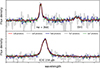 |
Fig. A.1. Zoomed-in view of a galaxy SED showing optical (top) and far-IR (bottom) spectral lines computed using different numbers of photon packets. |
Appendix B: SFR variation with inclination
We investigate the impact of the galactic viewing angle on the derivation of SFRs across different tracers. Figure B.1 compares the SFRs inferred from Hα, [C II], total IR luminosity, and hybrid (UV + IR) luminosities against the intrinsic SFRs averaged over 10 and 100 Myr. By varying the inclination from face-on to edge-on, we observe how dust attenuation and geometry affect the scatter and bias of these indicators which is further discussed in Sect. 4. Overall, the Hα-inferred SFR is the most sensitive to dust attenuation, showing an increasing scatter especially at 60° and edge-on configurations. In contrast, the other tracers show little to no dependence on viewing angle, highlighting their robustness against geometric effects and dust optical depths.
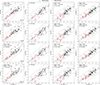 |
Fig. B.1. Left to right: SFR comparisons of Hα versus SFR10 Myr, [C II] at 158 μm versus SFR100 Myr, IR versus SFR 100Myr, and (UV + IR) versus SFR 100Myr for galaxies in the NEWCLUSTER (black squares) and NEWHORIZON (red circles) simulations. Each row corresponds to the different viewing angles: face-on, 30°, 60°, and edge-on (top to bottom). The solid gray line is the identity line, while the dashed, dotted and dash-dot lines indicate offsets of ±0.3, ±0.7, and ±1 dex, respectively. On the top left corner of each plot, the dispersion of the entire sample is shown. |
Appendix C: Leakage of UV photons: Effect on SFRIR scatter
The relationship between LIR and the SFR relies on the assumption that dust effectively absorbs and reprocesses UV radiation from young stars. To understand whether the scatter discussed in Sect. 4.2 is dominated by UV photon leakage, we explore the SFRIR − SFR100 Myr as a function of LIR/LFUV ratio. Figure C.1 shows that IR SFRs are systematically underestimated as LIR/LFUV ratio becomes smaller, and it is more pronounced for low-mass galaxies (NEWHORIZON). Conversely, sources with IR-to-UV ratios ∼1 are closer to the identity line. This highlights that UV-photon leakage contributes significantly to the scatter observed, particularly for underestimated SFRs. On the other hand, LIR/LFUV > 1 do not show a systematic offset and likely reflect effects such as stochastic star formation histories and stochastic heating of small dust grains, rather than UV leakage.
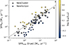 |
Fig. C.1. IR inferred SFRs versus time-averaged SFR over 100 Myr for NEWCLUSTER (squares) and NEWHORIZON (circles) simulated galaxies. We color code the data points based on the ratio of the total IR (8 − 1000 μm) and far-UV (1500 Å) luminosity (see Sect. 4.2 for details). |
Appendix D: Star Formation History: effect on LIR
We select sources from the simulations with the largest scatter in the SFRIR − SFR100 Myr plane (Fig. 5) with residuals larger than 0.5 dex, and derive the SFH over 200 Myr to inspect their burstiness at the galaxies’ young age (< 20 Myr). In Fig. D.1, we show in black and red the SFH of NEWCLUSTER and NEWHORIZON sources, respectively, which clearly display rising peaks of SFRs at t ∼ 10 Myr. The burstiness is seen to be stronger in lower mass galaxies from NEWHORIZON with M* < 109 M⊙, and a continuous decreases before stabilizing the rate of star formation in comparison to higher mass ones from NEWCLUSTER. For comparison, we also plot the SFH of sources from simulations with residuals < 0.2 dex in gray and light red, where the SFRs show a more stable evolution with time.
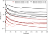 |
Fig. D.1. SFR as a function of lookback time relative to z = 5, shown over 200 Myr interval. The black and dark red lines corresponds to the NEWCLUSTER and NEWHORIZON sources, respectively, with SFRIR residuals > 0.5 dex. The gray and light red lines corresponds to the NEWCLUSTER and NEWHORIZON sources, respectively, with SFRIR residuals < 0.2 dex. (see Sect. 4.2 for details). |
Appendix E: SFR with updated attenuation curves
To evaluate the improvement provided by attenuation modeling, we compare the Hα-inferred SFRs using the dust attenuation ratio derived in Sect. 5.2. Figure E.1 displays the results using the standard Calzetti et al. (2000) law and our updated curves, which displays a tighter correlation between Hα-inferred SFRs and the intrinsic SFR10 Myr and a significant decrease in the scatter compared to the canonical attenuation curve. Nevertheless, a systematic offset is observed for intrinsically higher SFRs, leading to their underestimation by a factor of ∼2.
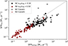 |
Fig. E.1. Hα-inferred SFRs versus 10 Myr time-averaged SFR. NEWHORIZON sources are shown in red circles, while NEWCLUSTER ones are shown in black squares. The solid colors indicate the SFRs inferred using the attenuation curves derived in Sect. 5.2 with kHα/kHβ = 0.58, while transparent colors denote SFRs inferred with Calzetti et al. (2000) attenuation law. The dashed line represents the identity line. |
All Tables
All Figures
|
Fig. 1. Projection of the gas mass (left) and post-processed SKIRT output of the Hα (middle) and [C II] (right) emission of the most and least massive NEWCLUSTER (top two rows) and NEWHORIZON (bottom two rows) galaxies in a face-on configuration. The bar shows the physical scale of each source in kiloparsec. |
| In the text | |
|
Fig. 2. Integrated spectral energy distribution of one representative NEWCLUSTER galaxy as produced by the SKIRT radiative transfer simulations assuming a DTM ratio of 16%. Left: Full SED in the observed frame, shown for the face-on (black) and edge-on (teal) configurations, spanning wavelengths from the ultraviolet to the millimeter. The shaded vertical regions show the coverage of ALMA bands 3, 7, and 9, and the dashed line demonstrates the JWST IFU range. Right: Examples of continuum-subtracted emission lines extracted from the same SED. |
| In the text | |
|
Fig. 3. Hα-derived SFRs using Eq. (3) vs. SFR10 Myr for NEWCLUSTER (black squares) and NEWHORIZON (red circles) simulated galaxies in a face-on configuration. The identity line is shown in black, and the dotted purple and orange lines show the best-fit of the Hα-derived SFRs using the conversion of Reddy et al. (2022) and Murphy et al. (2011), respectively (see Sect. 4.1 for details). In the top left corner, the slopes and offsets are shown with the same color code as the lines, and the scatter σ of the inferred SFRs. |
| In the text | |
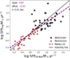 |
Fig. 4. Same as Fig. 3 for an edge-on viewing angle. |
| In the text | |
|
Fig. 5. Same as Fig. 3 for the IR-inferred SFRs vs. time-averaged SFR over 100 Myr. The SFRs are derived using Kennicutt (1998) conversion (Eq. (6)), and the best fit is shown by the dashed purple line. |
| In the text | |
|
Fig. 6. Same as Fig. 3 for the hybrid-inferred SFRs (IR + UV) vs. time-averaged SFR over 100 Myr. The SFRs are derived using the conversion in Eq. (7), and the best fit is shown by the dashed purple line. |
| In the text | |
|
Fig. 7. [C II] luminosity as a function of SFR100 Myr of NEWHORIZON- and NEWCLUSTER-simulated sources shown as circles and squares, respectively. The data points are color-coded based on the median of gas metallicities (left), the median of gas densities (middle), and the peak temperature (right) in a given source (see Sect. 4.4 for details). The dash-dotted black line shows the L[C II] − SFR relation we obtained. The dash-dotted purple, dotted blue, red, dashed green, and dashed magenta lines represent L[C II] − SFR relations by Olsen et al. (2017, z = 6), Lagache et al. (2018, z = 5), Schaerer et al. (2020, 4 < z < 6), Harikane et al. (2020, 6 < z < 9), and Accard et al. (2025, 4 < z < 6), respectively. |
| In the text | |
|
Fig. 8. Effect of DTEM on SFR estimates of Hα vs. SFR10 Myr, [C II] at 158 μm vs. SFR100 Myr, IR vs. SFR100 Myr, and gybrid (UV+IR) vs. SFR100 Myr (left to right) for NEWCLUSTER (squares) and NEWHORIZON (circles) simulated galaxies. The DTM ratios considered are 16% (black), 25% (blue), and 40% (orange). The solid gray line is the identity line, and the dashed, dotted, and dash-dotted lines indicate offsets of ±0.3, ±0.7, and ±1 dex, respectively. In the top left corner of each plot, the dispersion of the entire sample is shown. |
| In the text | |
|
Fig. 9. Left: Ratio of the Hα and Hβ attenuation laws derived vs. the Hα attenuation for NEWHORIZON (circles) and NEWCLUSTER (squares) simulated galaxies. Black, blue, and orange represent DTM ratios of 16%, 25%, and 40%, respectively. The ratio derived for simulated galaxies from Tacchella et al. (2022) (dashed gray line) and Kapoor et al. (2024) (dash-dotted teal line) and that derived by Calzetti et al. (2000) (dashed blue line) for local starbursts are shown. Right: Distribution of the derived attenuation law ratios for our sources at different DTM ratios. |
| In the text | |
|
Fig. 10. [C II]/IR luminosity ratios vs. IR luminosity of NEWCLUSTER (squares) and NEWHORIZON (circles). We color-code our sources based on the median gas metallicity (left) and median gas density (right) of each galaxy. We plot the observed ALPINE z ∼ 4 − 6 sources in purple (Schaerer et al. 2020) for comparison. |
| In the text | |
|
Fig. 11. Infrared luminosities derived using different approaches vs. the IR luminosity derived in Sect. 6 for our entire sample. The black squares show LIR derived using a modified blackbody, the red circles show LIR derived from the monochromatic luminosity from ALMA band 9, and blue stars show those derived from the monochromatic luminosity from ALMA band 7. The black line is the identity line, and the dashed black, solid red, and dotted blue lines represent the best fit of each inferred LIR. |
| In the text | |
|
Fig. A.1. Zoomed-in view of a galaxy SED showing optical (top) and far-IR (bottom) spectral lines computed using different numbers of photon packets. |
| In the text | |
|
Fig. B.1. Left to right: SFR comparisons of Hα versus SFR10 Myr, [C II] at 158 μm versus SFR100 Myr, IR versus SFR 100Myr, and (UV + IR) versus SFR 100Myr for galaxies in the NEWCLUSTER (black squares) and NEWHORIZON (red circles) simulations. Each row corresponds to the different viewing angles: face-on, 30°, 60°, and edge-on (top to bottom). The solid gray line is the identity line, while the dashed, dotted and dash-dot lines indicate offsets of ±0.3, ±0.7, and ±1 dex, respectively. On the top left corner of each plot, the dispersion of the entire sample is shown. |
| In the text | |
|
Fig. C.1. IR inferred SFRs versus time-averaged SFR over 100 Myr for NEWCLUSTER (squares) and NEWHORIZON (circles) simulated galaxies. We color code the data points based on the ratio of the total IR (8 − 1000 μm) and far-UV (1500 Å) luminosity (see Sect. 4.2 for details). |
| In the text | |
|
Fig. D.1. SFR as a function of lookback time relative to z = 5, shown over 200 Myr interval. The black and dark red lines corresponds to the NEWCLUSTER and NEWHORIZON sources, respectively, with SFRIR residuals > 0.5 dex. The gray and light red lines corresponds to the NEWCLUSTER and NEWHORIZON sources, respectively, with SFRIR residuals < 0.2 dex. (see Sect. 4.2 for details). |
| In the text | |
|
Fig. E.1. Hα-inferred SFRs versus 10 Myr time-averaged SFR. NEWHORIZON sources are shown in red circles, while NEWCLUSTER ones are shown in black squares. The solid colors indicate the SFRs inferred using the attenuation curves derived in Sect. 5.2 with kHα/kHβ = 0.58, while transparent colors denote SFRs inferred with Calzetti et al. (2000) attenuation law. The dashed line represents the identity line. |
| In the text | |
Current usage metrics show cumulative count of Article Views (full-text article views including HTML views, PDF and ePub downloads, according to the available data) and Abstracts Views on Vision4Press platform.
Data correspond to usage on the plateform after 2015. The current usage metrics is available 48-96 hours after online publication and is updated daily on week days.
Initial download of the metrics may take a while.