| Issue |
A&A
Volume 710, June 2026
|
|
|---|---|---|
| Article Number | A59 | |
| Number of page(s) | 9 | |
| Section | The Sun and the Heliosphere | |
| DOI | https://doi.org/10.1051/0004-6361/202659390 | |
| Published online | 03 June 2026 | |
Spatial distribution and physical characteristics of decomposed sunspot wave modes
1
Korea Astronomy and Space Science Institute, 776 Daedeok-daero, Yuseong-gu, Daejeon 34055, Republic of Korea
2
Astronomy Program, Department of Physics and Astronomy, Seoul National University, Seoul 08826, Republic of Korea
3
Astronomy and Space Science, University of Science and Technology, 217 Gajeong-ro, Yuseong-gu, Daejeon 34113, Republic of Korea
4
National Astronomical Observatory of Japan, 2-21-1 Osawa, Mitaka, Tokyo 181-8588, Japan
5
Research Institute of Natural Sciences, Chungnam National University, 99 Daehak-ro, Yuseong-gu, Daejeon 34134, Republic of Korea
6
Astronomy Research Center, Seoul National University, Gwanak-gu, Seoul 08826, Republic Korea
★ Corresponding author: This email address is being protected from spambots. You need JavaScript enabled to view it.
Received:
10
February
2026
Accepted:
21
April
2026
Abstract
Sunspot oscillations consist of multiple wave modes, making it challenging to isolate individual physical processes. To decompose these multi-modal oscillations, we apply empirical mode decomposition (EMD) to Hα Doppler velocity data obtained with the Fast Imaging Solar Spectrograph. By avoiding arbitrary frequency filtering, EMD resolves the oscillations into four distinct modes with unique periodicities and spatial distributions: c1 in the umbra (periods of ∼2 min); c2 in the umbra and penumbra (2.5 − 4 min); c3 in the outer penumbra (4 − 6 min); and c4 in the superpenumbra (∼10 min). We find that all modes, including the high-frequency 1-minute oscillations, coexist in the superpenumbral fibrils and represent potential candidates for transverse waves. Analysis of the c1 and c2 modes reveals the coexistence of umbra-trapped body waves and running penumbral waves within the umbra. Meanwhile, the c3 and c4 modes demonstrate that sunspot waves undergo significant nonlinear evolution as they propagate through the stratified atmosphere. Our results indicate that EMD effectively classifies dispersive oscillations into distinct groups based on their intrinsic timescales and underlying physical natures.
Key words: magnetohydrodynamics (MHD) / waves / Sun: chromosphere / Sun: oscillations / sunspots
© The Authors 2026
 Open Access article, published by EDP Sciences, under the terms of the Creative Commons Attribution License (https://creativecommons.org/licenses/by/4.0), which permits unrestricted use, distribution, and reproduction in any medium, provided the original work is properly cited.
This article is published in open access under the Subscribe to Open model. This email address is being protected from spambots. You need JavaScript enabled to view it. to support open access publication.
1. Introduction
Oscillations and waves in sunspots have attracted much attention since their first detection in 1969 (Beckers & Tallant 1969). Sunspot waves exhibit different characteristics depending on their spatial locations. The oscillations in the umbra, referred to as umbral oscillations, have dominant periods of around 3 minutes in the chromosphere (Beckers & Schultz 1972) and 5 minutes in the photosphere (Bhatnagar et al. 1972). The umbral oscillations are considered to be longitudinal slow magnetoacoustic waves propagating upward along the vertical magnetic field lines (Centeno et al. 2006). Sometimes the umbral oscillations appear to propagate radially outward across the vertical magnetic field, forming ring-like patterns (Zhao et al. 2015; Cho & Chae 2020) or spiral-shaped patterns (Sych & Nakariakov 2014; Kang et al. 2019, 2024b). These patterns have been interpreted either as fast waves that originate from local events in the subphotospheric high-β region, and convert into slow ones at the equipartition layer (Zhao et al. 2015; Kang et al. 2019; Cho & Chae 2020), or as a superposition of body modes (Stangalini et al. 2022; Kang et al. 2024a).
The oscillations in the penumbra with periods of about 5 minutes exhibit apparent radial outward propagation, known as running penumbral waves (RPWs; Giovanelli 1972). This radial propagation is well understood as a manifestation of slow magnetoacoustic waves propagating along expanding magnetic field lines (Kobanov et al. 2006; Bloomfield et al. 2007). To reach a given detection height, waves propagating along inclined magnetic fields must traverse a longer path than those in vertical fields. Consequently, wavefronts guided by vertical fields arrive earlier than those along inclined fields, producing the apparent outward propagation. Meanwhile, the predominant period of RPWs gradually increases with distance from the umbra (e.g. Maurya et al. 2013). This period change is well explained by the decrease in the acoustic cutoff frequency as the magnetic field inclination increases (Bel & Leroy 1977; Jess et al. 2013). Thus, 5-minute RPWs are often considered to share a common source with the 3-minute umbral oscillations near the umbral boundary, with the gradual period increase being a consequence of the increasing field inclination (Jess et al. 2013; Maurya et al. 2013). Alternatively, the 5-minute RPWs may originate from the merging of 3-minute shock waves originating in the umbra, which occurs when a trailing shock catches up with the preceding shock (Chae et al. 2015).
In the superpenumbral fibrils, transverse oscillations spanning a wide range of periods are detected using both imaging methods (Pietarila et al. 2011; Morton et al. 2021) and spectroscopic methods (Chae et al. 2021b, 2022). Morton et al. (2021) interpreted these transverse oscillations as kink waves propagating along the fibrils, with periods of around 10 minutes, and Chae et al. (2022) identified that the transverse oscillations can be classified into two groups with periods of approximately 3 and 10 minutes. Although the origin of these transverse waves remains a subject of debate, they are likely generated either through the conversion of p-mode (acoustic) fast waves into magnetic fast waves that are finally converted into Alfvénic modes (Morton et al. 2021) or via the slow-to-Alfvén mode conversion of longitudinal 3-minute waves (Chae et al. 2022). Recent studies have found that the transverse oscillations can be elliptically polarized, implying that the total energy flux may be significantly larger than previous estimates based on single-direction amplitude measurements (Bate et al. 2024; Kwak et al. 2025).
To analyze power spectra or to filter specific period bands in time series data, most wave studies have utilized Fourier-based techniques, such as the Fourier transform or wavelet transform. Although these methods are widely used, they have several limitations. First, Fourier-based techniques are founded on trigonometric functions, which strictly require the input time series to be both linear and stationary. While these methods can decompose nonlinear oscillations, such as shock waves, they often unintentionally incorporate multiple harmonics. These superfluous harmonics subsequently complicate the interpretation of the underlying oscillation characteristics. Therefore, the resulting power spectra must be interpreted with caution and appropriate theoretical consideration (Jess et al. 2023). Second, Fourier filtering introduces a degree of arbitrariness in selecting a specific period range. For example, to isolate umbral 3-minute oscillations, Kang et al. (2019) used a filtering range of 5.5–9 mHz, Cho & Chae (2020) adopted a broader range of 4–8 mHz, and Centeno et al. (2006) applied a much narrower range of 6–7 mHz. Since these filtering ranges are inherently user-dependent, the direct comparison of wave characteristics across different studies remains challenging.
To overcome these limitations of Fourier-based techniques, Huang et al. (1998) developed a statistical tool named empirical mode decomposition (EMD), which can decompose a time series into intrinsic timescales without assuming any mathematical basis functions. For this reason, the EMD can be applied to nonlinear and nonstationary data, such as shock waves. Furthermore, because the EMD is a data-driven method without any predefined basis functions, it is free from the arbitrariness of selecting specific period ranges for filtering. With these advantages, the EMD has been applied to coronal oscillations to avoid the leakage of wave energy across harmonic frequencies (Terradas et al. 2004), and to sunspot oscillations to analyze the spatial distribution of magnetic waveguides (Sych & Yan 2025).
One of the limitations of EMD is its sensitivity to noise. When the input data contains non-negligible noise, either distinct wave modes fail to be decomposed into separate modes, or a signal wave can be decomposed into multiple different modes. This phenomenon is referred to as “mode mixing” (Wu & Huang 2009). To address this issue, Wu & Huang (2009) developed the ensemble EMD method, which overcomes mode mixing by averaging the modes obtained from an ensemble of data with added white noise. As a result, the ensemble EMD is more suitable for wave studies involving systematic random noises (Jafarzadeh et al. 2025).
The purpose of this study is to investigate the characteristics of the individual modes and their spatial distribution by applying the ensemble EMD to sunspot waves. To achieve this, we analyzed time series of the chromospheric line-of-sight (LoS) Doppler velocity derived from the Hα spectra, obtained using the Fast Imaging Solar Spectrograph (FISS; Chae et al. 2013) at the Goode Solar Telescope. Consequently, we identified four oscillation modes, each of which exhibits a unique spatial distribution.
2. Data and methods
In this study, we analyzed a sunspot in the NOAA active region (AR) 13798 near the disk center (41″, 17″), observed with the FISS on 2024 August 25 from 19:05:09 to 20:26:10 UT. The observation was interrupted from 19:53:43 to 19:55:14 UT due to an adaptive optics unlock, resulting in a 90-second gap. As a result, the data were divided into two continuous segments with durations of 48 and 31 minutes, respectively. Fig. 1 shows raster images of the observed sunspot at Hα + 4 Å and at the Hα line center at 19:44:57 UT. The time cadence was 24 seconds, with a spatial sampling of 0.16″ and a spectral sampling of 19 mÅ. The field of view (FoV) was 33″ × 40″, covering the entire sunspot, including part of the superpenumbral fibrils. The data were calibrated following the FISS data reduction pipeline (Chae et al. 2013; Kang et al. 2025). To correct the field rotation, the images were derotated and subsequently aligned via cross-correlation of consecutive continuum images obtained at a wavelength of Hα + 4 Å.
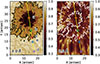 |
Fig. 1. Photospheric and chromospheric raster images of a sunspot, NOAA AR 13798, obtained at Hα + 4 Å and at the Hα line center, respectively, observed on 2024 August 25 at 19:44:57 UT. Black and white contours represent the boundaries of the umbra and penumbra, respectively. The yellow line denotes the slit position used for the time-distance map analysis shown in Fig. 5. Colored “+” symbols mark the five positions used to investigate the temporal variation in the LoS Doppler velocity and their corresponding EMD modes: (a) umbra (orange), (b) penumbra (green), (c) penumbral boundary (red), (d) outer superpenumbra (purple), and (e) inner superpenumbra (blue). |
To obtain the Doppler velocity oscillations across the entire FoV, we first calculated the chromospheric LoS Doppler velocity at each spatial pixel and time step using the multilayer spectral inversion technique (Chae et al. 2020, 2021a). Subsequently, we decomposed the LoS Doppler velocity time series for each pixel by applying ensemble EMD to both continuous data segments, following the ensemble approach of Wu & Huang (2009) and the original EMD formulation described by Terradas et al. (2004). For the ensemble average, the EMD was repeated N times, adding random white noise with a standard deviation of σ to the input time series in each trial. The true i-th mode, i.e., intrinsic mode function denoted as ci, was then defined as the average of the corresponding modes across all ensemble trials:
 (1)
(1)
Here, we set N = 200 and σ = 0.2 km s−1. We used only the first four EMD modes because higher-order modes exhibited very small amplitudes in our data.
To investigate the spatial distribution of each EMD mode, we determined the representative amplitude and period for every spatial pixel. The amplitude was defined as the root-mean-square (RMS) value of the extrema. The period (P) was calculated as the weighted average of the time intervals (pi) between consecutive peaks, weighted by the local squared amplitude (ai2), expressed as P = (∑ai2pi)/(∑ai2). Here, ai was obtained by averaging the magnitude of two consecutive peaks. Consequently, the square of the velocity amplitude corresponds to the oscillation power, and the period is more heavily weighted toward oscillations with more power.
3. Results
3.1. Characteristics of EMD
Fig. 2 shows the comparison between the original LoS Doppler velocity time series (top panels) with the four decomposed modes (subsequent four panels) at the four positions marked in the same colors in Fig. 1: (a) umbra (orange), (b) penumbra (green), (c) penumbral boundary (red), and (d) outer superpenumbra (purple). Unlike the original time series, all modes have a zero mean over the entire time domain, as the quasi-steady components are decomposed into the residual (Huang et al. 1998). The first mode, c1, shows the shortest period, and the higher the mode number, the longer the period becomes. Furthermore, the period of each mode is not constant but varies over time. This is consistent with the EMD algorithm, which extracts high-frequency components first by identifying the upper and lower envelopes of local extrema. Consequently, each mode represents a specific frequency band rather than a single monochromatic period.
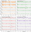 |
Fig. 2. Time series of the LoS Doppler velocity at the four locations marked in Fig. 1, and the resulting modes decomposed via EMD. The colors of the curves correspond to the same colors of the four locations marked in Fig. 1. For each location, the top panel shows the original time series, and the subsequent four panels show the EMD modes from c1 to c4. Time 0 denotes the start of the observation corresponding to 19:05:09 UT. The gray area at around 50 minutes represents the observing time gap. The negative value in velocity represents the upward motion (i.e., blueshift). Note that the y axes are scaled differently in each panel. |
A notable feature is that the decomposed modes preserve the nonlinearity of the input data. For instance, as is shown in Fig. 2c between t = 50 and 70 min, the original time series clearly shows the sawtooth patterns of nonlinear shock waves. These nonlinear features are also found and preserved in the c3 mode. This demonstrates that EMD is an effective tool for decomposing oscillations while maintaining their intrinsic nonlinear characteristics.
Another interesting feature is that EMD can decompose a single wave packet into multiple constituent components. This feature is evident in Fig. 2a. For example, between t = 50 and 80 min, the original oscillation appears as a single extended wave packet. The EMD successfully resolves this packet into the c1 and c2 modes. Given that these decomposed components have similar periods, they would likely remain indistinguishable under conventional broadband Fourier filtering. These characteristics of the EMD help one to identify and analyze underlying wave modes that would otherwise be obscured by waves with dominant power.
Fig. 3 shows the scatter plots of the period versus the amplitude for each decomposed mode. Here, red points indicate data within the umbra, green within the penumbra, and blue in the superpenumbra. To reduce sample density, the data points were averaged over ten adjacent pixels with similar amplitudes and periods across the FoV. The decomposed modes are well clustered, showing no mutual overlap between different modes. These results demonstrate that EMD effectively classifies the modes based on their distinct wave characteristics and intrinsic timescales.
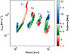 |
Fig. 3. Logarithmic scatter plot of RMS velocity amplitude versus period for all EMD modes. Color indicates the distance from the umbral center (marked with an orange symbol in Fig. 1): red points represent data from the umbra, green data from the penumbra, and blue data from the superpenumbra. The four specific locations marked in Fig. 1 are also indicated on the color bar. To improve clarity and reduce sample density, data from every ten adjacent pixels with similar amplitudes and periods are averaged. Some data points in the superpenumbra are partially obscured by those from the penumbra. |
3.2. Spatial distribution
As shown in Fig. 2, the EMD modes exhibit spatial variability in the dominant power of oscillations. To clearly examine the spatial distribution of each mode across the observed FoV, we applied the EMD method to every pixel and derived the dominant amplitude and period maps (Fig. 4). These maps demonstrate that the c1 mode is primarily confined to the umbra, the c2 mode resides between the umbra and penumbra, the c3 mode spans the penumbral boundary, and the c4 mode is found in the superpenumbra. Consequently, the EMD method can simply classify the sunspot waves into at least four different oscillation modes.
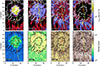 |
Fig. 4. Maps of the velocity amplitude (top) and period (bottom) on a logarithmic scale for each EMD mode. The columns from left to right correspond to an increasing mode number, from c1 to c4. White contours in the top row and black contours in the bottom row denote the boundaries of the umbra and penumbra. |
3.2.1. c1 mode
The c1 mode is confined within the umbra, exhibiting periods of 2 − 2.5 minutes (first column of Fig. 4). A small portion of these oscillations extends slightly beyond the umbral boundary, with their amplitude rapidly diminishing to the noise level. This confinement is also clearly visible in the time-distance map (t − d map, Fig. 5a) and the corresponding amplitude plot (Fig. 5b), obtained along the yellow line in Figs. 1 and 4. In the t − d map, the oscillations typically manifest as C-shaped ridges showing the apparent outward propagation. As is indicated by the lime boxes, the t − d map often exhibits dislocations characterized by zero amplitude in time while the oscillations at adjacent points are in antiphase. These dislocations indicate the existence of the nonzero azimuthal mode (López Ariste et al. 2013, 2016).
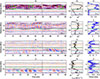 |
Fig. 5. Time-distance maps (left), RMS velocity (middle), and period (right) along the yellow slit marked in Fig. 1, for each EMD mode. The EMD modes are arranged in rows in increasing order from c1 to c4. Dashed black lines indicate the umbral boundaries, and each colored line corresponds to the positions marked with the same colors in Fig. 1. In panel (a), lime boxes mark the region where dislocations occur. Cyan circles in panel (g) represent shock merging regions. Lime-colored slopes and their associated values in panel (j) indicate the apparent propagation speeds derived from the slopes. The color scale for the time-distance maps ranges from –5 to 5 km s−1. As in Fig. 2, the observation start time is set to 0, and the gray areas represent intervals with missing data. Distance 0 corresponds to point “a” in Fig. 1. |
3.2.2. c2 mode
The c2 mode oscillations are observed across both the umbra and the penumbra (second column of Fig. 4). The RMS velocity amplitude of these oscillations remains relatively constant, while their period gradually increases from 3 minutes in the umbra to 5 minutes in the penumbra. Meanwhile, the t − d map in Fig. 5d shows that the oscillations appear to propagate outward from the umbra to the outer penumbra, forming the characteristic C-shaped ridges. All of these results are consistent with the properties of the RPWs (Jess et al. 2013).
3.2.3. c3 mode
The c3 mode oscillations are primarily distributed in the outer penumbra (third column of Fig. 4), with a dominant period of approximately 5 minutes. Their amplitude peaks at the penumbral boundary; meanwhile, the period gradually increases from 4 to 6 minutes across the penumbra before decreasing in the superpenumbra. The scatter plot of c3 mode (Fig. 3) also clearly shows this positive correlation between amplitude and period as a function of distance from the umbra to the penumbral boundary (see red and green-colored data points). Beyond the boundary, both values decrease.
The c3 mode occasionally shows shock merging features. For instance, cyan circles in the t − d map (Fig. 5g) mark shock merging points where two red ridges merge into a single ridge during their outward propagation. Concurrently, Fig. 2c reveals that these oscillations evolve into shocks, as characterized by sawtooth patterns. These nonlinear characteristics are consistent with shock merging processes previously reported in a pore (Chae et al. 2015).
3.2.4. c4 mode
The c4 mode is observed exclusively within the superpenumbra, with periods ranging from 8 to 14 minutes (fourth column of Fig. 4). In the scatter plot (Fig. 3), both the amplitude and period decrease from the umbral center toward the umbral boundary, after which they both increase with radial distance, extending up to 15 Mm.
The c4 mode likely represents RPWs propagating along highly inclined fields. As shown in Fig. 2d, the oscillations before t = 40 min show sinusoidal fluctuations, yet they exhibit nonlinear features showing inverse sawtooth patterns in the inner superpenumbra (Fig. 6). Between t = 40 and 70 min, the waves show nonlinear sawtooth patterns similar to those observed at the penumbral boundary. Interestingly, the slopes of the ridges in Fig. 5j increase from 16 to 65 km s−1 during the time interval of 10–40 min. These high-speed values may be interpreted as apparent speeds rather than the actual propagation speed of the waves.
3.2.5. Minor modes in the superpenumbra
In addition to the spatially distributed dominant modes, all decomposed modes are detected in the superpenumbra (top panels in Fig. 4). The c1 mode is found in the superpenumbra with periods of approximately 1 minute, and this mode does not appear to be physically connected to the umbral oscillations. Similarly, the c2 mode is detected in the superpenumbra with a period of roughly 3 minutes, appearing to be intermittently connected with the oscillations in the penumbra. The c3 mode is also identified in the superpenumbra with periods of approximately 4 minutes. In the t − d maps (Fig. 5), all these superpenumbral oscillations show vertical ridges indicating the fast propagation speeds or standing waves similar to previous reports (Chae et al. 2021b).
Among the identified modes, the c1 oscillations are well clustered in the scatter plot with periods of approximately 1 minute (blue points in Fig. 3). These high-frequency oscillations appear consistent with the transverse waves with an Alfvénic nature. They are detected far from the sunspot center, where magnetic field lines are highly inclined. In such a geometry, transverse oscillations can be identified in the LoS direction. Notably, while the oscillation period remains constant, the amplitude increases with distance from the penumbral boundary (Figs. 5b and c). This amplitude enhancement likely results from the projection effect; as the field line becomes more inclined, the transverse oscillations align more closely with the LoS direction. Furthermore, Fig. 5a reveals nearly vertical ridges in the superpenumbra, indicating a high propagation speed. Taken together, these characteristics suggest that the high-frequency c1 oscillations in the superpenumbra may be associated with transverse waves of an Alfvénic nature.
4. Discussion
We analyzed the LoS Doppler velocity oscillations within a sunspot using the ensemble EMD method, which avoids arbitrary frequency filtering. This method naturally resolves the sunspot waves into four distinct modes, each characterized by a specific period range. Given the dispersive nature of sunspot waves, each decomposed mode exhibits unique physical behaviors in terms of propagation and spatial distribution. Consequently, EMD facilitates the investigation of individual wave modes by automatically grouping them based on both their periodicity, with distinct physical properties, as illustrated in the schematics (Fig. 7). In this section, we discuss the plausible origins of each wave mode based on observed characteristics.
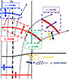 |
Fig. 7. Schematic illustration of each EMD mode. Thin solid black lines in the background represent the magnetic field configuration, while the thick black line denotes the photospheric surface. Dashed and dotted black lines indicate the umbral and penumbral boundaries, respectively. Blue and red curves represent the wavefronts of the c1 and c2 modes, respectively. The cyan circle highlights the shock merging region. The dark red line near the penumbral boundary illustrates the leading shock front, where the preceding wavefront (red line) merges. Bidirectional arrows indicate the direction of oscillations: blue for c1, red for c2, purple for merged-shock oscillations, yellow for convection-driven kink oscillations, and navy for p-mode-driven kink oscillations. |
4.1. Origin of c1 mode
The confinement of the c1 mode can be explained by two plausible mechanisms: upward wave propagation along inclined field lines or the presence of body waves. Regarding the former, the expansion of the magnetic field in the penumbra increases the acoustic cutoff period; consequently, while waves with periods longer than the timescale of the c1 mode are enhanced, the power of the c1 mode itself diminishes in these regions. This magnetic geometry also suggests that the C-shaped ridges observed in the t − d map could be an apparent propagation, where wavefronts reaching the chromosphere experience a time delay as they travel along increasingly inclined fields (Löhner-Böttcher & Bello González 2015).
Alternatively, the c1 mode may originate from body waves trapped within the umbra (illustrated by the blue wavefronts in Fig. 7). As was described by Edwin & Roberts (1983), such oscillations are confined within a flux tube and decay exponentially with distance from its boundary. This confinement is expected, as the field strength and other physical quantities change abruptly at the umbral boundary, causing wave reflection. This interpretation is supported by recent studies that have identified multiple eigenmodes of body waves in umbrae (e.g. Jess et al. 2017; Kang et al. 2019; Stangalini et al. 2022). In our observations, we identified signatures of nonzero azimuthal modes in the form of dislocations in the t − d map (Fig. 5a), one of the indicators of body wave characteristics (López Ariste et al. 2016). Furthermore, the C-shaped ridges can be interpreted as a superposition of higher-order radial modes, where the slope of the ridges varies depending on the relative contribution of the higher-order modes (Kang et al. 2024a). Thus, the observed variation in ridge slopes can be attributed to changes in the amplitude ratios of higher-order modes. Therefore, the observed characteristics of c1 can be explained by body waves trapped within the sunspot umbra.
4.2. Origin of c2 mode
It is particularly interesting that the umbral oscillations comprise both the umbra-trapped c1 mode and the c2 mode, the latter of which contributes to the RPWs. Previous studies have often considered the umbral oscillations and the RPWs as slow waves originating from a common source, with the period difference attributed to the varying magnetic field inclination (e.g. Bloomfield et al. 2007; Jess et al. 2013). In contrast, Kobanov et al. (2006) suggested that 3-minute umbral oscillations are unlikely to leak into RPWs, as they were not evident in the time-distance maps filtered in the 3-minute band. However, our EMD analysis distinctly decomposes the umbral oscillations into two wave modes. This decomposition suggests that the origin of the c1 may differ from that of the c2 mode (illustrated by the red wavefronts in Fig. 7).
The detection of the c2 mode in the umbra raises questions regarding its underlying driving mechanism. Similar to the c1 mode, the c2 mode could be associated with the upward-propagating waves. In Fig. 5d, the slope of the ridges changes abruptly at the umbral boundary, indicating a sharp transition in magnetic field inclination within the penumbra. If the c2 waves were propagating along the same inclined umbral field as c1, their ridges in the t − d map would be expected to exhibit a similar or even more bent curvature; this is because low-frequency waves have a slower propagation speed, making them more susceptible to geometric time delays. However, this expectation contradicts our observations, where the c2 ridges remain relatively straight. This discrepancy suggests that an additional physical process is responsible for the origin of the c2 mode.
Here, we propose that the c2 mode represents body waves confined within the penumbral boundary, originating from the subphotosphere rather than simple plane waves. According to Kang et al. (2024a), the number of trapped radial modes decreases as the oscillation period increases, which potentially allows higher-order radial modes to leak outward. If some of these leaked modes become trapped within the penumbra beneath the photosphere, they may subsequently contribute to the RPWs. Furthermore, the distinction between umbra and penumbra becomes ambiguous at depths exceeding 7 Mm, where overturning convection is enhanced against the vertical magnetic field (Schmassmann et al. 2021). Thus, the c2 mode can be generated by waves trapped near the penumbral boundary in the deep subphotosphere. If this is true, the c2 ridges within the umbra would appear to be relatively straight compared to those of the c1 mode, as the higher-order radial components of c2 leak out from the umbra. Further studies, including numerical simulations, are necessary to fully elucidate the driving mechanisms underlying these c2 oscillations.
4.3. Origin of c3 mode
As is described in Sect. 3.2.3, the c3 mode shows the characteristics of nonlinearly evolved slow waves. This suggests that these oscillations can be interpreted as nonlinear RPWs that have developed into shock waves. As slow waves propagate upward, their amplitude increases due to density stratification. Once the amplitude exceeds a critical threshold determined by the local sound speed, the waves undergo acoustic steepening and finally evolve into shocks (e.g. Chae & Litvinenko 2017).
The green box in Fig. 7 illustrates an alternative mechanism for the c3 mode: the merging of the 3-minute shock waves (Chae et al. 2015). Assuming two shock waves propagate along the inclined field, when a trailing shock overtakes a preceding one, the two shocks can merge into a single enhanced shock with a larger amplitude and longer period. This mechanism aligns well with our observations of the c3 mode, which shows a distinct nonlinear signature in the time series and also clear merging features.
4.4. Origin of c4 mode
Similar to the c3 mode, the c4 mode can be associated with RPWs propagating along highly inclined field lines (illustrated by the purple box in Fig. 7). These oscillations intermittently exhibit nonlinear features, suggesting an acoustic nature (Figs. 2d and 6). Under the RPWS interpretation, the high apparent propagation speeds measured in the t − d map can be attributed to the geometric effect of wavefronts propagating along the inclined field lines. Alternatively, such high apparent speeds may be related to the depth of the wave-driving source (Zhao et al. 2015; Cho & Chae 2020). According to Zhao et al. (2015), if quasi-isotropic acoustic waves are excited beneath a sunspot, wavefronts reaching more distant regions arrive later due to their longer travel paths, thereby creating an apparent outward propagation with enhanced speeds. Consequently, a deeper source results in a faster apparent speed, as the difference in path lengths is minimized for waves originating from greater depths (Cho & Chae 2020). Therefore, we suggest that the evolution of the wavefronts observed in Fig. 5j between t = 10 and 40 min is more likely attributable to variations in the depth of the excitation source rather than changes in the field inclination.
4.5. Origin of minor modes in the superpenumbra
If the minor modes within the superpenumbra are indeed the transverse waves, they may be interpreted as kink waves in superpenumbral fibrils, exhibiting Alfvénic characteristics. As is shown in Fig. 1, the superpenumbra consists of numerous dark and bright fibrils. Furthermore, the oscillation power in this region is localized, tracing the fibrillar structures (Fig. 4). This spatial correlation supports the idea that these waves are confined in the inhomogeneous magnetic structures. These findings are quite consistent with the kink waves previously identified in the superpenumbral fibrils (Morton et al. 2021; Chae et al. 2021b). Therefore, the minor modes observed in the superpenumbra are likely waves confined in fibrils.
The c2 and c3 modes may potentially be generated through various mode conversion processes. First, shock-mediated slow-to-Alfvén mode conversion could drive these transverse oscillations with the periods of 3–5 minutes (Chae et al. 2022). In regions where shock waves locally enhance the plasma β within the strongly curved magnetic field, the mode conversion process becomes effective in triggering transverse oscillations. Alternatively, direct slow-to-Alfvén conversion in high-β regions could also generate 3-minute transverse oscillations (Chae et al. 2022). Furthermore, Morton et al. (2021) suggested that photospheric p-mode excited fast waves could be converted into the Alfvénic modes.
The origin of the 1-minute c1 mode in the superpenumbra remains mysterious, as its period is shorter than both the acoustic cutoff of other typical sunspot oscillations. The lack of spatial continuity between this superpenumbral mode and the umbral source suggests that its origin may not be associated with the umbral oscillations. Considering high-frequency oscillations observed in other regions (e.g. He et al. 2009; Morton et al. 2013; Chae et al. 2025), we propose three potential mechanisms for their excitation. First, these high-frequency oscillations may be driven by photospheric convective motions. In the quiet Sun fibrils, Morton et al. (2013) found that photospheric convection-driven vortex flows are strongly coupled with chromospheric high-frequency transverse oscillations, leading to the conclusion that such vortex motions can drive these oscillations. In our case, photospheric motions near the sunspot or at remote footpoints could potentially trigger these transverse oscillations.
The second plausible mechanism involves the nonlinear generation of harmonics by upward-propagating longitudinal shock waves. As acoustic waves undergo steepening due to density stratification, they generate higher-order harmonics at increased frequencies. These high-frequency components can subsequently undergo mode conversion into transverse oscillations, such as fast or Alfvén waves (Khomenko & Cally 2012; Shoda & Yokoyama 2018). However, as this process is primarily transient, it may be limited in explaining the persistent nature of the observed oscillations.
A third possibility is the harmonics of standing kink modes (Gao et al. 2023). In short coronal loop simulations, an inclined p-mode driver at a footpoint can excite standing kink oscillation harmonics with periods of approximately 1 minute (Gao et al. 2023; Skirvin et al. 2023). While this scenario can account for persistent high-frequency oscillations of an Alfvénic nature, it remains to be determined whether these coronal results can be directly applied to chromospheric superpenumbral fibrils. Further studies are required to fully understand the origin of these high-frequency oscillations and their role in atmospheric heating.
5. Conclusions
In this work, we investigated the complex nature of sunspot oscillations by applying the ensemble EMD method to LoS Doppler velocity data. Unlike conventional Fourier-based filtering, EMD allowed us to decompose overlapping wave signals based on their intrinsic timescales without arbitrary frequency filtering. The EMD method successfully resolved the sunspot waves into four distinct modes (c1 to c4), each exhibiting unique spatial distributions and propagation behaviors. By analyzing c1 and c2 modes, we identified that umbral oscillations consist of two distinct types of slow waves: umbral trapped body waves and waves contributing to RPWs. The c3 and c4 modes provided clear evidence of nonlinear steepening and shock interaction, as these nonlinear features are well preserved within the decomposed modes. Furthermore, we uncovered high-frequency oscillations in the superpenumbral fibrils that appear to be excited independently of shock wave activity. Collectively, these results demonstrate that sunspot oscillations comprise various wave modes that can be spatially grouped with distinct physical natures.
Ultimately, the identification of these diverse wave modes, especially the high-frequency and transverse components, helps us to understand the chromospheric heating. To further quantify the contribution of each mode to chromospheric heating, further studies utilizing high-resolution observations and numerical simulations will be essential.
Acknowledgments
We appreciate all constructive comments given by an anonymous referee. This work was supported by the Korea Astronomy and Space Science Institute under the R&D program of the Korean government (MSIT; No. 2026-1-830-05). J. C. was supported by the National Research Foundation of Korea (RS-2023-00208117). H.K. was supported by Basic Science Research Program through the National Research Foundation of Korea(NRF) funded by the Ministry of Education(RS-2024-00452856) K.-S. L. was supported by the National Research Foundation of Korea (RS-2025-23523356). The GST operation is partly supported by the Korea Astronomy and Space Science Institute and the Seoul National University. BBSO operation is supported by US NSF AGS-2309939 grant and New Jersey Institute of Technology.
References
- Bate, W., Jess, D. B., Grant, S. D. T., et al. 2024, ApJ, 970, 66 [NASA ADS] [CrossRef] [Google Scholar]
- Beckers, J. M., & Schultz, R. B. 1972, Sol. Phys., 27, 61 [NASA ADS] [CrossRef] [Google Scholar]
- Beckers, J. M., & Tallant, P. E. 1969, Sol. Phys., 7, 351 [NASA ADS] [CrossRef] [Google Scholar]
- Bel, N., & Leroy, B. 1977, A&A, 55, 239 [NASA ADS] [Google Scholar]
- Bhatnagar, A., Livingston, W. C., & Harvey, J. W. 1972, Sol. Phys., 27, 80 [Google Scholar]
- Bloomfield, D. S., Lagg, A., & Solanki, S. K. 2007, ApJ, 671, 1005 [NASA ADS] [CrossRef] [Google Scholar]
- Centeno, R., Collados, M., & Trujillo Bueno, J. 2006, ApJ, 640, 1153 [Google Scholar]
- Chae, J., & Litvinenko, Y. E. 2017, ApJ, 844, 129 [Google Scholar]
- Chae, J., Park, H.-M., Ahn, K., et al. 2013, Sol. Phys., 288, 1 [NASA ADS] [CrossRef] [Google Scholar]
- Chae, J., Song, D., Seo, M., et al. 2015, ApJ, 805, L21 [NASA ADS] [CrossRef] [Google Scholar]
- Chae, J., Madjarska, M. S., Kwak, H., & Cho, K. 2020, A&A, 640, A45 [NASA ADS] [CrossRef] [EDP Sciences] [Google Scholar]
- Chae, J., Cho, K., Kang, J., et al. 2021a, J. Korean Astron. Soc., 54, 139 [Google Scholar]
- Chae, J., Cho, K., Nakariakov, V. M., Cho, K.-S., & Kwon, R.-Y. 2021b, ApJ, 914, L16 [NASA ADS] [CrossRef] [Google Scholar]
- Chae, J., Cho, K., Lim, E.-K., & Kang, J. 2022, ApJ, 933, 108 [CrossRef] [Google Scholar]
- Chae, J., Lim, E.-K., Kang, J., Lee, K.-S., & Madjarska, M. S. 2025, A&A, 698, A259 [NASA ADS] [CrossRef] [EDP Sciences] [Google Scholar]
- Cho, K., & Chae, J. 2020, ApJ, 892, L31 [NASA ADS] [CrossRef] [Google Scholar]
- Edwin, P. M., & Roberts, B. 1983, Sol. Phys., 88, 179 [Google Scholar]
- Gao, Y., Guo, M., Van Doorsselaere, T., Tian, H., & Skirvin, S. J. 2023, ApJ, 955, 73 [NASA ADS] [CrossRef] [Google Scholar]
- Giovanelli, R. G. 1972, Sol. Phys., 27, 71 [NASA ADS] [CrossRef] [Google Scholar]
- He, J.-S., Tu, C.-Y., Marsch, E., et al. 2009, A&A, 497, 525 [NASA ADS] [CrossRef] [EDP Sciences] [Google Scholar]
- Huang, N. E., Shen, Z., Long, S. R., et al. 1998, Proc. R. Soc. Lond. Ser. A, 454, 903 [Google Scholar]
- Jafarzadeh, S., Jess, D. B., Stangalini, M., et al. 2025, Nat. Rev. Methods Primers, 5, 21 [Google Scholar]
- Jess, D. B., Reznikova, V. E., Van Doorsselaere, T., Keys, P. H., & Mackay, D. H. 2013, ApJ, 779, 168 [Google Scholar]
- Jess, D. B., Van Doorsselaere, T., Verth, G., et al. 2017, ApJ, 842, 59 [Google Scholar]
- Jess, D. B., Jafarzadeh, S., Keys, P. H., et al. 2023, Liv. Rev. Sol. Phys., 20, 1 [NASA ADS] [CrossRef] [Google Scholar]
- Kang, J., Chae, J., Nakariakov, V. M., et al. 2019, ApJ, 877, L9 [NASA ADS] [CrossRef] [Google Scholar]
- Kang, J., Chae, J., Cho, K., Kang, S., & Lim, E.-K. 2024a, A&A, 686, A293 [NASA ADS] [CrossRef] [EDP Sciences] [Google Scholar]
- Kang, J., Chae, J., & Geem, J. 2024b, ApJ, 960, 115 [NASA ADS] [CrossRef] [Google Scholar]
- Kang, J., Song, D., Chae, J., Lim, E.-K., & Kubo, M. 2025, J. Korean Astron. Soc., 58, 63 [Google Scholar]
- Khomenko, E., & Cally, P. S. 2012, ApJ, 746, 68 [Google Scholar]
- Kobanov, N. I., Kolobov, D. Y., & Makarchik, D. V. 2006, Sol. Phys., 238, 231 [Google Scholar]
- Kwak, H., Lim, E.-K., Chae, J., et al. 2025, A&A, 700, A133 [NASA ADS] [CrossRef] [EDP Sciences] [Google Scholar]
- Löhner-Böttcher, J., & Bello González, N. 2015, A&A, 580, A53 [NASA ADS] [CrossRef] [EDP Sciences] [Google Scholar]
- López Ariste, A., Collados, M., & Khomenko, E. 2013, Phys. Rev. Lett., 111, 081103 [Google Scholar]
- López Ariste, A., Centeno, R., & Khomenko, E. 2016, A&A, 591, A63 [NASA ADS] [CrossRef] [EDP Sciences] [Google Scholar]
- Maurya, R. A., Chae, J., Park, H., et al. 2013, Sol. Phys., 288, 73 [Google Scholar]
- Morton, R. J., Verth, G., Fedun, V., Shelyag, S., & Erdélyi, R. 2013, ApJ, 768, 17 [Google Scholar]
- Morton, R. J., Mooroogen, K., & Henriques, V. M. J. 2021, Philos. Trans. R. Soc. Lond. Ser. A, 379, 20200183 [Google Scholar]
- Pietarila, A., Aznar Cuadrado, R., Hirzberger, J., & Solanki, S. K. 2011, ApJ, 739, 92 [NASA ADS] [CrossRef] [Google Scholar]
- Schmassmann, M., Rempel, M., Bello González, N., Schlichenmaier, R., & Jurčák, J. 2021, A&A, 656, A92 [NASA ADS] [CrossRef] [EDP Sciences] [Google Scholar]
- Shoda, M., & Yokoyama, T. 2018, ApJ, 854, 9 [CrossRef] [Google Scholar]
- Skirvin, S. J., Gao, Y., & Van Doorsselaere, T. 2023, ApJ, 949, 38 [NASA ADS] [CrossRef] [Google Scholar]
- Stangalini, M., Verth, G., Fedun, V., et al. 2022, Nat. Commun., 13, 479 [NASA ADS] [CrossRef] [Google Scholar]
- Sych, R., & Nakariakov, V. M. 2014, A&A, 569, A72 [NASA ADS] [CrossRef] [EDP Sciences] [Google Scholar]
- Sych, R., & Yan, Y. 2025, ApJ, 986, 180 [Google Scholar]
- Terradas, J., Oliver, R., & Ballester, J. L. 2004, ApJ, 614, 435 [Google Scholar]
- Wu, Z., & Huang, N. E. 2009, Adv. Adapt. Data Anal., 1, 1 [CrossRef] [Google Scholar]
- Zhao, J., Chen, R., Hartlep, T., & Kosovichev, A. G. 2015, ApJ, 809, L15 [NASA ADS] [CrossRef] [Google Scholar]
All Figures
|
Fig. 1. Photospheric and chromospheric raster images of a sunspot, NOAA AR 13798, obtained at Hα + 4 Å and at the Hα line center, respectively, observed on 2024 August 25 at 19:44:57 UT. Black and white contours represent the boundaries of the umbra and penumbra, respectively. The yellow line denotes the slit position used for the time-distance map analysis shown in Fig. 5. Colored “+” symbols mark the five positions used to investigate the temporal variation in the LoS Doppler velocity and their corresponding EMD modes: (a) umbra (orange), (b) penumbra (green), (c) penumbral boundary (red), (d) outer superpenumbra (purple), and (e) inner superpenumbra (blue). |
| In the text | |
|
Fig. 2. Time series of the LoS Doppler velocity at the four locations marked in Fig. 1, and the resulting modes decomposed via EMD. The colors of the curves correspond to the same colors of the four locations marked in Fig. 1. For each location, the top panel shows the original time series, and the subsequent four panels show the EMD modes from c1 to c4. Time 0 denotes the start of the observation corresponding to 19:05:09 UT. The gray area at around 50 minutes represents the observing time gap. The negative value in velocity represents the upward motion (i.e., blueshift). Note that the y axes are scaled differently in each panel. |
| In the text | |
|
Fig. 3. Logarithmic scatter plot of RMS velocity amplitude versus period for all EMD modes. Color indicates the distance from the umbral center (marked with an orange symbol in Fig. 1): red points represent data from the umbra, green data from the penumbra, and blue data from the superpenumbra. The four specific locations marked in Fig. 1 are also indicated on the color bar. To improve clarity and reduce sample density, data from every ten adjacent pixels with similar amplitudes and periods are averaged. Some data points in the superpenumbra are partially obscured by those from the penumbra. |
| In the text | |
|
Fig. 4. Maps of the velocity amplitude (top) and period (bottom) on a logarithmic scale for each EMD mode. The columns from left to right correspond to an increasing mode number, from c1 to c4. White contours in the top row and black contours in the bottom row denote the boundaries of the umbra and penumbra. |
| In the text | |
|
Fig. 5. Time-distance maps (left), RMS velocity (middle), and period (right) along the yellow slit marked in Fig. 1, for each EMD mode. The EMD modes are arranged in rows in increasing order from c1 to c4. Dashed black lines indicate the umbral boundaries, and each colored line corresponds to the positions marked with the same colors in Fig. 1. In panel (a), lime boxes mark the region where dislocations occur. Cyan circles in panel (g) represent shock merging regions. Lime-colored slopes and their associated values in panel (j) indicate the apparent propagation speeds derived from the slopes. The color scale for the time-distance maps ranges from –5 to 5 km s−1. As in Fig. 2, the observation start time is set to 0, and the gray areas represent intervals with missing data. Distance 0 corresponds to point “a” in Fig. 1. |
| In the text | |
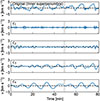 |
Fig. 6. Similar to Fig. 2, but for the position of the inner superpenumbra marked blue in Fig. 1. |
| In the text | |
|
Fig. 7. Schematic illustration of each EMD mode. Thin solid black lines in the background represent the magnetic field configuration, while the thick black line denotes the photospheric surface. Dashed and dotted black lines indicate the umbral and penumbral boundaries, respectively. Blue and red curves represent the wavefronts of the c1 and c2 modes, respectively. The cyan circle highlights the shock merging region. The dark red line near the penumbral boundary illustrates the leading shock front, where the preceding wavefront (red line) merges. Bidirectional arrows indicate the direction of oscillations: blue for c1, red for c2, purple for merged-shock oscillations, yellow for convection-driven kink oscillations, and navy for p-mode-driven kink oscillations. |
| In the text | |
Current usage metrics show cumulative count of Article Views (full-text article views including HTML views, PDF and ePub downloads, according to the available data) and Abstracts Views on Vision4Press platform.
Data correspond to usage on the plateform after 2015. The current usage metrics is available 48-96 hours after online publication and is updated daily on week days.
Initial download of the metrics may take a while.