| Issue |
A&A
Volume 700, August 2025
|
|
|---|---|---|
| Article Number | A223 | |
| Number of page(s) | 19 | |
| Section | Stellar structure and evolution | |
| DOI | https://doi.org/10.1051/0004-6361/202349083 | |
| Published online | 26 August 2025 | |
Discovery of young, oxygen-rich supernova remnants in PHANGS-MUSE galaxies
1
European Southern Observatory, Alonso de Córdova 3107, Casilla 19, Santiago, Chile
2
Tuorla Observatory, Department of Physics and Astronomy, FI-20014 University of Turku, Finland
3
Finnish Centre for Astronomy with ESO (FINCA), FI-20014 University of Turku, Finland
4
Millennium Institute of Astrophysics MAS, Nuncio Monsenor Sotero Sanz 100, Off. 104, Providencia, Santiago, Chile
5
Department of Astronomy, Kyoto University, Kitashirakawa-Oiwake-cho, Sakyo-ku, Kyoto 606-8502, Japan
6
School of Sciences, European University Cyprus, Diogenes Street, Engomi, 1516 Nicosia, Cyprus
⋆ Corresponding author: This email address is being protected from spambots. You need JavaScript enabled to view it.
Received:
22
December
2023
Accepted:
1
April
2025
Abstract
Context. Supernova remnants (SNRs) are the late stages of supernovae (SNe) before they merge to the surrounding medium. Oxygen-rich (O-rich) SNRs represent a rare subtype with strong visible-light oxygen emission.
Aims. We present a new method to detect SNRs exploiting the capabilities of modern visible-light integral-field units based on the shapes of the SNR emission lines.
Methods. We search for unresolved shocked regions with broadened emission lines using the medium-resolution integral-field spectrograph MUSE on the Very Large Telescope. The spectral resolving power allows shocked emission sources to be differentiated from photoionised sources based on the linewidths.
Results. We find 307 SNRs, including seven O-rich SNRs. For all O-rich SNRs, we observe the [O III]λλ4959,5007 emission doublet. In addition, we observe emissions from [O I]λλ6300,6364, [O II]λλ7320,7330, Hα+[N II]λ6583 and [S II]λλ6717,6731 to varying degrees. The linewidths for the O-rich SNRs are generally broader than the rest of the SNRs in the sample of this article. The oxygen emission complexes are reminiscient of SNR 4449-1 and some long-lasting SNe. For the O-rich SNRs, we also search for counterparts in archival data of other telescopes; we detect X-ray and mid-IR counterparts for a number of remnants.
Concluions. We have shown the efficacy of the method in detecting SNRs presented in this article. In addition, the method is also effective in detecting the rare O-rich SNRs, doubling the sample size in the literature. The origin of O-rich SNRs and their link to specific SN types or environments is still unclear, but further work into this new sample will unquestionably help us shed light on these rare remnants.
Key words: supernovae: general / galaxies: ISM
© The Authors 2025
 Open Access article, published by EDP Sciences, under the terms of the Creative Commons Attribution License (https://creativecommons.org/licenses/by/4.0), which permits unrestricted use, distribution, and reproduction in any medium, provided the original work is properly cited.
This article is published in open access under the Subscribe to Open model. This email address is being protected from spambots. You need JavaScript enabled to view it. to support open access publication.
1. Introduction
Supernova remnants (SNRs) are the last evolutionary phase of supernovae (SNe) before they merge into the surrounding interstellar medium (ISM). They exhibit complex interactions between the ejecta and any significant circumstellar medium (CSM) together with the ISM. In the case of core-collapse SNe, additional luminosity may arise from the compact central object – a neutron star or a black hole – due to magnetic breaking or accretion. These interactions give rise to signatures of shocked gases, most notably of hydrogen, nitrogen and sulphur. The timescale of this phase is from thousands of years to a million years (Micelotta et al. 2018).
Oxygen-rich supernova remnants (O-rich SNRs) are objects with strong observed oxygen features. The prototypical O-rich SNR is Cassiopeia A, which has knots dominated by [O III] λλ4959,5007 (Milisavljevic et al. 2012). However, to date very few O-rich remnants are known. In the Milky Way (MW) and the Magellanic Clouds there are eight such objects. These are Cassiopeia A, Puppis A and G292+1.8 in the MW, 0540-69.3 and LMC N132D in the Large Magellanic Cloud (LMC), 1E 0102.2-7219, B0049-73.6 and B0103-72.6 in the Small Magellanic Cloud (Vogt & Dopita 2010; Schenck et al. 2014). The latter two have no published optical-wavelength spectra. However, both have X-ray observations that show enhanced oxygen abundances. This low number of O-rich SNRs is in stark contrast to the around 300 SNRs discovered in the MW1. From the literature, only one object designated as an O-rich SNR outside the MW system is found; SNR 4449-1 in NGC 4449. SNR 4449-1 was originally detected in the radio (Seaquist & Bignell 1978), then subsequently in the optical (Balick & Heckman 1978) and in X-rays (Blair et al. 1983). The optical spectra examined in Balick & Heckman (1978) showed a similarity between the SNR and the O-rich knots of Cas A and N132D, a remnant in the LMC.
Some long-lasting SNe show similar spectral features to SNR 4449-1. These include SN 1957D in M83, SN 1979C in M100 and SN 1995N in MCG-02-38-017 (Long et al. 2012; Milisavljevic & Fesen 2008; Wesson et al. 2023). SN1980K also has strong oxygen emission lines (Milisavljevic et al. 2012). A sample of late-time observations of SNe can be found in Milisavljevic et al. (2012). Blair et al. (2015) also find an ejecta-dominated SNR in M83 labeled B12-174a with broad Hα, [S II]λλ6717,6731 and weaker oxygen lines. More recently, Caldwell & Raymond (2023) report a discovery of the SNR labeled WB92-26 with strong nitrogen and oxygen lines that they dubbed a ‘N-rich SNR’.
There is an apparent connection between dust formation and O-rich remnants. Cas A has clear infrared (IR) excesses implying the presence of dust. For example, Cas A has been estimated to host 0.5 M⊙ of silicate dust, with carbon dust formation being quenched due to the O-rich nature of the remnant (De Looze et al. 2017). Based on modeling of optical emission line profiles, Niculescu-Duvaz et al. (2022) estimate dust masses for SN 1979C to be ≈0.3–0.65 M⊙. SNR 4449-1 and other O-rich SNRs have also been detected at X-ray wavelengths. Patnaude & Fesen (2003) report a total luminosity of 2.4 × 1038 erg/s for SNR 4449-1, an order of magnitude more luminous than Cas A, and comparable to the 6.5 × 1038 erg/s luminosity of SN 1979C, which has been argued to host a newly formed black hole (Patnaude et al. 2011).
The nature of O-rich SNRs and their connection to specific SNe is still unclear. While Cas A was spectroscopically identified as a type IIb (Krause et al. 2008), SN1979C was classified as an extremely bright type II with a fast declining light curve (de Vaucouleurs et al. 1981). Given the low number of known O-rich SNRs (nine in total), any additional discoveries and their subsequent characterisation can significantly aid in understanding these remnants and their progenitor properites. In addition, it appears that only a few SNe have been recovered years after the explosion. In these long-lasting SNe, strong oxygen and Hα features are often observed (Milisavljevic et al. 2012; Kuncarayakti et al. 2016), which could indicate a shared, but uncommon, evolutionary stage for certain core-collapse SNe.
In this paper, we introduce a new methodology for finding SNRs, report the discovery of new O-rich SNRs and characterise our sample of seven extragalactic O-rich remnants. We additionally compile a sample of ‘recovered SNe’ that we argue provide a strong link to O-rich remnants, perhaps indicating a common origin. In Section 2 we present our observations and data reductions. In Section 3 we describe our methods for finding SNRs with an integral-field spectrograph and search for counterparts in data obtained with other facilities. In Section 4 we show our results, then discussion and conclusions are presented in Sections 5 and 6 respectively.
2. Observations
The project presented in this paper was motivated by an initial search for shock-ionised regions in an optical-wavelength spectroscopic datacube of Messier 61 (NGC 4303). This led to the serendipitious discovery of two objects that appeared consistent with O-rich SNRs, particularly SNR 4449-1. Following this initial discovery, we initiated a systematic search for O-rich SNRs. The discovery was based on the Very Large Telescope Multi Unit Spectroscopic Explorer (MUSE, Bacon et al. 2010) observations of NGC 4303, data which are part of the PHANGS-MUSE program. The Physics at High Angular resolution in Nearby GalaxieS (PHANGS) survey uses Atacama Large Millimeter/submillimeter Array (ALMA, Leroy et al. 2021), Hubble Space Telescope (HST, Lee et al. 2022), James Webb Space Telescope (JWST, Lee et al. 2023) and MUSE (Emsellem et al. 2022) data to study small-scale physics of gas and star formation. These high-resolution observations allow for a wide range of studies as a spin-off from the original survey aims. We limit our search to this dataset, because it has some of the best spatial coverage of nearby galaxies. These data also guarantees HST observations for most of the galaxies (16 out of 19) and gives a reasonable coverage of JWST images - observations that are still ongoing. The proximity of these galaxies also gives a good archival Chandra X-ray coverage.
The MUSE data used are from European Southern Observatory (ESO) Program ID 1100.B-0651 (Emsellem et al. 2022). The observations were made in wide-field mode both with and without adaptive optics between November 2017 and February 2021. The data were retrieved from ESO Phase 3 archive2 and were reduced by the PHANGS-MUSE collaboration. For the four host galaxies of O-rich SNRs we searched archives of HST, JWST and Chandra for supporting material. The datasets used are described in Appendix C. We downloaded the Level 3 reduced data from the Mikulski Archive for Space Telescopes (MAST)3. The HST observations are partially based on PHANGS-HST observations (Lee et al. 2022). For HST observations we used DOLPHOT to measure the magnitudes of our targets. With JWST data we employed jdaviz4 and CIAO for the Chandra datasets (JDADF Developers et al. 2023; Fruscione et al. 2006).
In addition to the archival data for our O-rich SNRs, we also downloaded reduced spectra of WB92-26 observed with Multiple Mirror Telescope (MMT) Hectospec in October 2006, November 2006, and October 2007 were downloaded from the MMT/Hectospec M31 archive5. Reduced spectra of SNR 4449-1 observed with HST FOS in January 1993 were downloaded from MAST. Reduced spectrum of SN 1979C observed with Gemini-N GMOS in May 2017 was downloaded from WISeREP6. Spectra of SNR 0540-69.3 were extracted from a MUSE observation that was part of the ESO program ID 0102.D-0769 observed between January and March 2013. The data were downloaded from ESO Phase 3 archive.
3. Methods
In this section we first review the traditional, historic methods of detecting extragalactic SNRs. We then describe our new methodology that makes use of the large field of view (FOV) integral field unit (IFU) capabilities of the MUSE instrument. We define the steps needed to go from a reduced MUSE datacube to a list of unresolved broad-line regions and finally to a list of SNR candidates. At the end of the section we present our methodology as applied to one galaxy in the dataset.
3.1. Identification of SNRs
A classic method to find SNRs is to measure the line ratio of [S II]/Hα, with a ratio higher than 0.4 being interpreted to be a likely SNR (Smith et al. 1993; Matonick & Fesen 1997). However, it has been noted that this method might not be exhaustive and could omit some SNRs, e.g. coinciding HII regions producing strong Hα emission that could skew the line ratio (Blair & Long 1997). Also, Cid Fernandes et al. (2021) reports several SNRs with [S II]/Hα ratio lower than 0.4. This line-ratio method has been often used as it enables searches for SNRs over large FOVs (e.g. the full extent of large – on the sky – nearby galaxies) through the use of narrow-band filters. So while emission line ratios can be used to differentiate between different emission mechanisms, such as photoionization or shock excitation, the measured ratios can differ significantly from the empirical values. Thus, other detection methods should be investigated in order to recover a more complete picture of SNR populations.
With new technologies (such as IFUs) it is now possible to obtain additional, spatially resolved spectral information for all regions of galaxies with a single pointing. With MUSE, we can observe a whole galaxy in spectral space at high enough resolution in order to allow us to develop and test new tools to discover SNRs. We expect SNRs to have ejecta velocities of over 200 km/s up to 100 kyr after the SN explosion (Micelotta et al. 2018) see their figure 1), which is in a stark contrast to the typical thermal velocities of HII regions of 10–20 km/s (Fernández Arenas et al. 2018). Planetary nebulae have similar velocities of few tens of km/s caused by the expansion of the nebula (Schönberner et al. 2018). The broader nature of emission lines produced in SNRs can therefore be used to separate and identify such objects from other emission-line sources. With IFU data, we can use a combination of line ratios and velocities to isolate and identify SNRs.
Following the availability of MUSE IFU data and the possibility to use velocity information to find SNRs, we proceeded to search for broadened emission lines using narrow-line off center images. The emission lines used in this survey generally do not have strong absorption lines associated with them in the stellar continua. Therefore, a simple linear approximation for the continuum subtraction was considered sufficient to detect broad-line emissions without the need to consider contamination from absorption lines. These line maps then show the presence of broadened emission lines. Sources for these regions include: shocked sources such as SNRs, but additionally HII regions with high S/N producing large full width at zero intensity, emission-line stars and late-type stars with a complex continuum. These latter stars can be in the host galaxy or appear as foreground stars. In Section 3.2 we outline how we differentiate between these different sources.
The broadened-emission-line maps produced above contain both unresolved point sources and extended emission regions. The remnants are a few to tens of parsecs in size and appear as unresolved sources at the distances in our MUSE dataset, between 9 and 20 Mpc, or 0.37″–0.85″for an SNR with diameter of 37 pc (i.e. something the size of the Cygnus Loop; Fesen et al. 2018). Extended emission sources are large HII regions or emission from diffuse ISM. To identify unresolved point sources, we processed the maps through SExtractor (Bertin & Arnouts 1996). The result of this method is presented in Fig. 1 for NGC 4303. We then extracted the point source spectra from the original MUSE datacube based on the resulting coordinates and removed the background continua with annular rings around the sources. Shock-powered region sources are generally easily identifiable by eye due to distinctly broadened emission lines and enhanced [S II]λλ6717,6731 emission, but we also measured the line ratios of Hα, [N II]λ6583 and [S II]λλ6717,6731 in order to confirm the identified shocked regions. In addition, we required all of the aforementioned lines to be detected in order to be considered a regular SNR; for O-rich SNRs we forfeited this requirement. We note that broad sources with log(Hα/[S II]) < 0.4 are most likely SNRs, but also that this cutoff is empricial, as discussed previously. Thus, we inspected sources near this cutoff more closely.
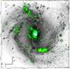 |
Fig. 1. Colour image of M61 compiled from three narrow-line maps used in this survey; red, green and blue colours correspond to [SII], Hα and [OIII], respectively. The background image is the collapsed cube of the MUSE observation. White circles and numbers are the SNRs in the galaxy confirmed by this survey. Magenta stars indicate the locations of previously observed SNe in the field of view. Gold stars show the locations of the three O-rich SNRs in the galaxy. Corresponding stamps of the other host galaxies are available here. |
3.2. Application to NGC 4303
Martínez-Rodríguez et al. (2024) shows the effectiveness of using integral field spectroscopy to search for SNRs, using a conceptually similar technique to that which we have presented, i.e. identifying broadened emission regions. The authors note a lack of O-rich events in their sample. However, the total number of SNRs they discovered is much less than through our methods: 19 in their work compared with a total of more than 300 here, even though Martinez-Rodriguez et al. search for SNRs in a much larger galaxy sample (around a 1000 galaxies compared to the sample of 19 used here). The differences between the detection rates of these studies are likely related to the discovery techniques. While both search for broadened emission, Martínez-Rodríguez et al. (2024) only select the broadest (> 400 km/s) Hα components and therefore the youngest SNR candidates. They therefore ignore the possibility of detecting SNRs with broadened metal lines.
In this subsection we outline our methodology for finding new SNR candidates within MUSE datacubes of nearby galaxies using NGC 4303 as an example case. The datacube of this galaxy is a 3 × 3 MUSE mosaic centered on the galaxy cenntre (leading to a total field size of 3′×3′). Most of the extent of NGC 4303 was thus observed, however the outer spiral arm regions are outside of the FOV. Even though the galaxy is quite face-on, there is an inclination of 27° (Tschöke et al. 2000) which causes, along with the galaxy rotation, redshift and blueshift of the emission lines that is detectable within the MUSE data. To account for this shift, we inspect each cube, spaxel by spaxel, identifying Hα emission and fitting a Gaussian to it. By comparing the shift of the Gaussian mean with the Gaussian mean of the center of the galaxy, we produce a redshift map of the galaxy, describing the effect of the galaxy inclination. Using this redshift map we remove the galaxy rotational effects by estimating the spectral bin drift. In NGC 4303, the rotation causes a drift of ≈2 Å and in other galaxies this can be larger.
We now have our MUSE spectra of NGC 4303 with all spaxels wavelength corrected to a common reference – the galaxy centre. With this in hand, we proceeded to extract off-centered linemaps from the cube. Lines used and their respective bandwidths are listed in Table 1. For example, in the case of the [N II]λ6583 emission line, we extracted a linemap from the red side of the emission line. This linemap is centered at 6588 Å, so we selected the MUSE spectral bin that includes this wavelength as our central point. From this spectral bin, we selected a wavelength range that is 6.25 Å wide, or five spectral bins of 1.25 Å, thus from 6584.88 Å to 6591.13 Å. This range covers the wing of an emission line with a FWHM of about 350 km/s. This methodology is depicted in Fig. 2, as applied to the [S II]λλ6717,6731 doublet. The figure shows how the method applies to a shocked ionised SNR region and also a photoionised HII region, reiterating the point above - SNRs have broader lines the other emission-line sources. The final linemap is produced by summing the flux in the defined wavelength range. In the case of the [O III]λλ4959,5007 doublet, we did not expect to observe any emission lines between them. Therefore, we opted to use a wider bandwidth for the linemap in order to increase the S/N of the oxygen emission without the risk of being contaminated other emission lines.
Emission lines used in our survey, their sampled wavelengths and bandwidths.
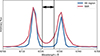 |
Fig. 2. Comparison of [SII]λλ6717,6731 emission lines from a SNR and an HII region, scaled to similar peak fluxes. The area bounded by black vertical lines (black arrows) is extracted and continuum subtracted. The difference in flux extracted between the two sources is apparent. |
Next, we estimated the continuum level to be extracted from the line maps. We did this using regions offset from the emission lines. In the case of [N II]λ6583, we centered them to wavelengths 6530 Å and 6630 Å. For all lines, we used regions offset by ±14 Å from the emission line centre to estimate the continuum at the emission-line wavelength. The continuum tends to be either very weak compared to the emission lines or almost linear in such a narrow passband, so we fit a simple linear continuum model to them. We subtracted this model continuum from the spectrum.
Following the above steps, we were now left with maps showing sources of broadened emission lines – unbroadened sources (e.g. most HII regions) have zero or near-zero flux following the continuum subtraction. Visually inspecting the newly produced continuum-subtracted linemap we could see some extended emission regions related to strong star-formation (for example the northern quadrant of NGC 4303 in Fig. 1). These are caused by high S/N of the emission lines. While the FWHM of an HII region is effectively constant and dominated by instrument broadening, bright HII regions might still have observable wings that bleed into our linemap. We also saw bright unresolved point sources in the maps, which are our points of interest.
For the next step we opted to use SExtractor in order to extract the coordinates of the point sources from the line maps; at this point we were only interested in the centroid of the point source. We iteratively changed the source extraction parameters until no obvious point source is missed in visual inspection. SExtractor produces a catalog of identified sources. Using this catalogue we then extracted the 1D spectra of these point sources from the original MUSE datacube. One spectrum is extracted using an aperture with a width of the seeing at the time of the observation, 0.8″ or 4 pixels in the case of NGC 4303. A second spectrum is extraced using an annular ring around the first extraction region with a size of 0.2″. The second spectrum is used to continuum-subtract the first. We were then left with continuum-subtracted 1D spectra of our point sources and SNR candidates. At these scales the diffuse emission from nearby HII regions and the stellar population is near-homogeneous. By scaling the amount of flux extracted by the ratio of spaxels in both the source aperture and the annulus, we can remove the HII contaminations with a direct subtraction.
With a list of SNR candidate spectra in hand, we visually inspected each one to identify their nature as true SNRs, contaminant HII regions or other sources. We fit Gaussian lines to visible strong lines, specifically Hα, [N II]λ6583 and [S II]λλ6717,6731, to measure their FWHM. Spectra that have self-consistent broadened emission lines, i.e. the detected lines of a given source all have similar FWHMs and are higher than 3 Å (135 km/s), were deemed to be originating from shocked regions and thus be SNRs. We also qualitatively note that these broadened emission sources tend to have stronger [N II]λ6583 and [S II]λλ6717,6731 emission compared to Hα, indicating a shocked source. HII regions contaminating this sample are identified by having emission line widths close to the instrument broadening, indicating photoionization sources. Star contaminants are identified either from their continua, e.g. M-type stars have metal lines such as TiO, or by the shape of the emission line; emission-line stars have strong hydrogen emission lines that have a Lorentzian profile or they show narrow CaIIλλλ8498,8542,8662 emission lines. This process was then repeated for all catalogues of every emission line used to produce the maps (i.e. [O III]5007, Hα, [N II]λ6583 and [S II]λλ6717,6731). In some cases, the same SNR was identified several times from different line maps. The final step is to then cross-match all the detected SNRs from all line maps based on their respective centroid coordinates. Our final product is then a full list of SNR candidates in NGC 4303. We then repeated these steps for all galaxies within our sample.
We found a total of 307 SNRs in our survey across all galaxies in our sample. Out of these, 35 SNRs had detected oxygen emission, with at minimum a detection in the [O III] linemap. This is to be expected as SNRs sometimes exhibit cooling lines such as the [O III]λλ4959,5007 doublet from the SNR interior (Makarenko et al. 2023). During the last visual inspection we also took note of the oxygen emission lines of [O III]λλ4959,5007, [O I]λλ6300,6364 and [O II]λλ7320,7330. From this subset, we noted that seven remnants in particular exhibit unusually strong and broad oxygen lines when compared to Hα, [N II]λ6583 and [S II]λλ6717,6731. We labeled these events as ‘O-rich SNRs’, and we characterise and discuss them in detail in Chapter 4.
3.3. Biases and restrictions
Before the SNR indentification process outlined in the previous subsection, we also needed to consider the completeness of our methodology and what types of false positives we may detect. We assumed that the interesting sources are point sources in the MUSE data. This is mostly fine for compact shocked sources such as young SNRs, but we also have a bias for detecting these. There might be objects with narrower emission lines that are closer to the MUSE spectral resolution, e.g. older SNRs, or there may be resolved objects such as the SNR Cygnus Loop. These latter objects might instead show up as arcs with relatively narrow emission lines, but with high peculiar velocity shift at different position angles of the arc.
We also expect to observe objects, such as emission-line stars, P-Cygni stars and Wolf-Rayet stars. All of these objects have strong broad Hα emission lines, with widths larger than a few hundred km/s. However, these will have very different emission profiles from shocked sources; emission-line stars generally have Lorentzian emission lines with narrow near-IR (NIR) CaII emission lines, while P-Cygni stars show typical blueshifted absorption features. Wolf-Rayet stars have a distinct ‘red bump’ at ∼5808 Å which is observable with MUSE (Gómez-González et al. 2021).
The extracted SNR spectra are shock-excited, meaning that the Case B condition for the estimation of extinction is not fulfilled. We therefore estimated extinctions based on the Balmer decrement and adopted the fluxes for Hα and Hβ from Emsellem et al. (2022) for the environments of each individual SNR. We calculated extinctions assuming reddening law value RV = 3.1 and adopted the model from Cardelli et al. (1989). This may cause inaccuracies as the colour excess is measured on larger scales and does not probe the intrinsic SNR extinction.
3.4. Counterparts at other wavelengths
After the identification of O-rich SNRs in our sample, we searched for counterparts in the archival data of other facilities. SN 1979C, another long-observed SN and SNR 4449-1 have been detected in X-rays (Patnaude et al. 2011; Patnaude & Fesen 2003), IR (Tinyanont et al. 2016) and radio (Weiler et al. 1981; Lacey et al. 2007; Bietenholz et al. 2010). Depending on the age of the remnants and the depth of archival data, we thus expect to find counterparts to these sources as well. We performed archival searches for HST, JWST and Chandra data using MAST and Chandra Data Archive (CDA)7.
For HST, we find that all O-rich SNR host galaxies have been observed with Wide Field Camera 3 with at least filters F275W, F336W, F438W, F555W and F814W, mostly due to PHANGS-HST and the Legacy ExtraGalactic UV Survey (LEGUS).
With JWST the observations for PHANGS-JWST are still ongoing as of writing; NGC 4303 has only partial coverage with the Near Infrared Camera (NIRCam) and does not include the positions of the O-rich SNRs in the galaxy. In the other cases NIRCam observations include filters F200W, F300M, F335M and F360M. JWST’s Mid-Infrared Instrument (MIRI) has observations with filters F770W, F1000W, F1130W and F2100W. In Chandra data, there are usually multiple epochs of data. We measured both the stacked flux and generated a lightcurve based on them. The former assumes a constant flux between the epochs and gives a more accurate flux measurement, while the latter assumes an evolving lightcurve. We used the coordinates from MUSE data and attempted to visually identify point sources in the datasets of other instruments. Absolute coordinate solutions in the publicly available PHANGS-MUSE dataset are validated against Gaia DR1 (Emsellem et al. 2022) and we expect World Coordinate System coordinates in the space telescope archival data to be accurate down to the image quality of MUSE observations, i.e. less than 0.8″.
In this section we have outlined our methodology for discovering new SNRs in our dataset, using NGC 4303 as an example. During the search, we discovered a total of seven unresolved sources, that have broad emission oxygen emission lines. In the following section we define our list of O-rich SNRs and proceed to characterise each event in terms of its observed features at optical wavelengths, compare them to a recovered SN and the prototypical O-rich SNR, SNR 4449-1. We will also discuss the counterparts detected at other wavelengths.
4. Results
Through the methodology outlined in the previous section, we found a total of 307 SNR candidates in the PHANGS-MUSE sample. All detected SNRs are listed in Appendix B. We leave a thorough analysis of this full sample for a future publication. For the newly discovered SNRs, we use a naming convention of SNR XXXX-YY, where XXXX is the galaxy number in the NGC/IC catalogues and YY is the running number of the SNR based on the declination from South to North. The SNRs are presented in Fig. 3 on an emission-line diagnostic plot. The SNR population on average exhibit [S II]λλ6717,6731 and [N II]λ6583 fluxes comparable to the Hα flux. We note a trend in the FWHM of the SNRs, where the linewidth tends to narrow as the SNR gets closer to the photoionized zone in the figure. The outlier remnant with log(Hα/[S II]) > 0.5 is the O-rich SNR 3627-17. For the rest of the O-rich SNRs, the emission lines are either too blended to measure accurately or too weak to detect. A total of seven SNRs (just 2% of the whole sample) exhibit optical emission line features reminiscient of young O-rich SNRs (see Fig. 4).
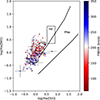 |
Fig. 3. Our sample of broadened emission lines that have detectable Hα, [N II]λ6583 and [S II]λλ6717,6731 emission lines and that we identify as SNRs. Colour of the points represent the FWHM of the [N II]λ6583 with the instrumental broadening removed. The different regions in the figure have been adopted from Meaburn et al. 2010. Most of our sample aligns with the SNR region with log(Hα/[S II]) < 0.5. |
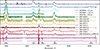 |
Fig. 4. Optical wavelength spectra of all seven O-rich SNRs discovered by our work. We addditionally display the spectra of three SNe at 15–40 years post explosion, SNR 4449-1, and also include a spectrum of SNR 0540-69.3, an old O-rich SNR in the LMC. |
We will discuss each O-rich remnant separately in the succeeding sections. In general, the remnants are heterogenous (as will be outlined below), showing different strength Hα and [S II] emission, but all of them have at least a detectable broad [O III] emission and sometimes also [OII] and [OI] emission lines (defining them as ‘O-rich’). We note that the spectrum of SNR 4449-1 is reminiscient of the O-rich SNRs presented in this paper to varying degrees. Similar features have also been observed in old SNe/young SNRs, including SN1957D, SN1979C, SN1980K, SN1996cr and SN1995N (Long et al. 2012; Fesen et al. 1999; Bauer et al. 2008; Wesson et al. 2023). We will compare all of our sources to both SNR 4449-1 and SN 1979C in the figures. The two sources are similar to each other and they are also most reminiscient to our O-rich SNRs. The spectra are scaled in order to highlight the spectral features and their similarities. We will describe the spectral features, possible counterpart detections and how they compare to other remnants and long-lasting SNe.
Searching the space-telescope archives MAST and CDA, we found that most of the sources have a Chandra counterpart, i.e. an unresolved source within 1″ of the object, (see example of NGC 4303 in Fig. 5). The luminosities for all sources range in the order of few 1037 − 1038 erg/s for these objects based on measurements outlined in Section 3.4 (see Table A.1). These are near the limit of ultra-luminous X-ray sources and around the Eddington limit of neutron star mass objects. These are also comparable to SN 1979C; LX = 6.5 × 1038 erg/s and SN 1957D; LX = 1.7 × 1037 erg/s (Long et al. 2012). HST counterparts are generally only detected in F555W and F814W, with weaker detection or non-detections in other filters such as the near-ultraviolet filter F275W. This seems to agree with previous observations of SNR 4449-1 where the dominant emission features are in visible/NIR oxygen lines (see Fig. 1 in Blair et al. 1983). In JWST we observe bright point sources at these remnant locations. The detections are presented in Fig. 6. Specifically SNR 4303-46 and SNR 3627-17 show very similar features compared to SN 1979C.
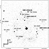 |
Fig. 5. X-ray image of NGC 4303 obtained with Chandra, observed in August 2001. None of the historical SNe have an associated source in X-ray, but both SNR 4303-46 and SNR 4303-20 are detected. SNR 4303-20 is considerably dimmer compared to SNR 4303-46, while SNR 4303-37 has very faint detection. |
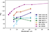 |
Fig. 6. JWST observations of the new O-rich SNRs compared to SN 1979C with JWST and SN 1995N from Wesson et al. (2023). |
Given the similarity between our discovered O-rich SNRs and old SNe/young SNRs, we searched for known SNe at the locations of our SNRs. However, no matches were found. SNR 4303-46 is near SN1926A, but the projected separation is over 5″, corresponding to a distance of 350 pc. We discuss this possible connection in detail below.
Now, we discuss each identified O-rich SNR in detail, characterising its optical-wavelength properties and noting detections at other wavelengths. A summary of the observed properties of our sample is presented in Appendix A.
4.1. SNR 4303-46
SNR 4303-46 was detected in the off-center linemaps in [O III] and Hα, being the brightest point source in the [O III] linemap of NGC 4303 (see Fig. 1). The MUSE spectrum (from 4700 Å to 9400 Å) is presented in Fig. 8. The most striking and dominant component observed is the [O III]λλ4959,5007 emission feature, which is brighter than the rest of the spectrum, defining it as an O-rich SNR. SNR 4303-46 also displays strong, broad lines of [O I]λλ6300,6364 and [O II]λλ7320,7330. A comparatively weak Hα+[N II]λ6583 is also visible, along with a marginal [S II]λλ6717,6731 detection.
The FWHM of the [O III]λλ4959,5007 complex is over 4000 km/s and is asymmetrical. We measure a total flux of 1.8 ± 0.3 × 1038 erg/s. Due to the high S/N of the spectrum we can see that the emission feature is a blend of several [O III] doublets with different velocities with respect to the assumed rest wavelength. Overall this is very similar to both SNR 4449-1 and SN 1979C, especially to the former.
In Fig. 9 we show the scaled [O III]λλ4959,5007 and [O I]λλ6300,6364 lines of SNR 4303-46, SNR 4449-1 and SN 1979C. SN 1979C’s emission lines are clearly blueshifted when centered at the host galaxy’s rest wavelengths (similar figures for the other O-rich SNRs are shown in Appendix D). This could be an indication of some O-rich outflows in SN1979C or an obstruction of the receding shell due to high dust extinction. Still, the red wings of SN 1979C’s and SNR 4303-46’s oxygen lines roughly trace each other, which suggests a similar origin, with SN 1979C only having excess blueshifted emitting material. Similarities to SNR 4449-1 are more clear, with the [O I]λλ6300,6364 lines having effectively the same shape. [O III]λλ4959,5007 lines are also similar, with SNR 4303-46 having a slight blueshifted excess and SNR 4449-1 exhibiting a red bump. Both also show a similar structure that could be explained with blueshifted and redshifted oxygen doublets as previously discussed by Milisavljevic & Fesen 2008. We measured a total flux of [O III]λλ4959,5007 for SNR 4449-1 of 4.6 × 1039 erg/s in the 1996 HST spectra. This is an order of magnitude brighter than SNR 4303-46.
SNR 4303-46 is also detected with HST, JWST and Chandra. Cutouts from HST and JWST images are available online here. We identify a strong point source in filter HST/F555W and JWST/F2100W slightly offset from the MUSE detection centerpoint. In all cases we observe a point source. From the HST images this limits the size of the source to 6 pc, which in turn limits the age of the SNR to less than a thousand years: assuming an ejecta that has a constant speed of 4000 km/s (based on the [O III] doublet) it would reach a radius of 3 pc in about 740 years. Considering the ejecta experiences only deceleration normal circumstances, this age would then be the upper limit for the age of the SNR.
Figure 6 shows the similarity between SN 1979C and SNR 4303-46 JWST SEDs along with our other O-rich sources that we have been detected in the JWST observations. Adopting a distance modulus of 31.03, SNR 4303-52 reaches MAB = −13.14 in F2100W. While SNR 4303-46 is two magnitudes fainter, the similarity in their overall shape is apparent. The slight plateau near the F1130W filter could be an indication of silicate dust, which has an absorption feature around 14 μm.
The SNR is also detected with Chandra in 2001 and 2014, as presentend in Table A.1 in Appendix A. The two epochs have very similar luminosities and by combining the two observations, we estimate a luminosity LX = 5.4 × 1038 erg/s. The same source is also likely observed by ROSAT between July 1996 and January 1998 with a luminosity of 4.3 ± 1.5 × 1038 erg/s; source g indentified in Tschöke et al. (2000) is consistent with the Chandra source when considering ROSAT’s lower spatial resolution. This is comparable to the Chandra observations and could be an indication that the source X-ray luminosity is constant over this period.
As is apparent in Fig. 5, our detection of SNR 4303-53 appears spatially close to the position of SN 1926A. Given that one of our hypothesis presented in this work is that our O-rich SNRs may be related – in time – with old SNe, we decided to further investigate a possible connection of these two events. SN 1926A was discovered and followed up by Max Wolf and Karl Reinmuth at the Heidelberg-Königstuhl State Observatory with the 72 cm Walz reflector telescope (Campbell 1926). The plates have been scanned and are available online8. We analysed a photographic plate dated May 11th 1926. Stars were identified on the old plate and matched to those with positions from Gaia data release 3 (Gaia Collaboration 2016, 2023) (Fig. 7). This provided an astrometric solution with a standard deviation of 1.5″ between the reported coordinates and the star locations. While this is quite a large, the distance between SNR 4303-53 and SN 1926A is 7.8″ which equates to a 5-sigma separation. We adopt new coordinates of RA = 12:21:59.67 Dec = +04:27:13.67 for SN 1926A. Following the above analysis, we do no believe that these to events are physically associated.
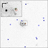 |
Fig. 7. Image of SN 1926A observed on May 11th 1926. We calibrated the coordinate solution based on stars observed by Gaia (blue circles). The SN location is identified (green circle) with the nearby SNR 4303-46 (red circle). The arrow length of the compass is 30″ in the inset. |
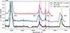 |
Fig. 8. Comparison of SNR 4303-46, SNR 4449-1 and SN 1979C. Solid lines are smoothed spectra, shaded represents the original spectrum. Vertical lines indicate different emission lines; [O III] (cyan), [O I] (magenta), Hα (red), [S II] (pink) and [O II] (yellow). |
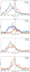 |
Fig. 9. [O III]λλ4959,5007 emission complex in velocity space centered around 5006.8 Å (top) and same for [O I]λλ6300,6364 centered around 6300 Å (second panel). The oxygen lines of SN1979C with the addition of [O II]λλ7320,7330 centered at 7320 Å (third panel) and the same lines for SNR 4303-5 (bottom panel). The spectra are normalized arbitrarily to have similar peak intensities. Corresponding figures to other O-rich SNRs are presented in Appendix D. |
4.2. SNR 4303-20
SNR 4303-20 was detected in all linemaps used in the survey. This is due to a strong Hα+[N II]λ6583 complex, along with strong [S II] and oxygen emission (see Fig. 10). These lines make the remnant to be somewhat reminiscient of a classical SNR, with the exception of the lines being broad: the Hα+[N II]λ6583 complex has a FWHM of about 3700 km/s, comparable to the oxygen lines observed in SNR 4303-46. This complex also seems to be blended; the [S II] doublet has a a total FWHM of about 1700 km/s. While the remnant’s oxygen lines are not the strongest emission sources in the MUSE spectrum they are nevertheless broad as well, with [O III]λλ4959,5007 doublet dominating over the less ionized oxygen lines. The [O III]λλ4959,5007 luminosity was measured to be 7.02 × 1036 erg/s, over two orders of magnitude lower than SNR 4303-46.
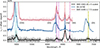 |
Fig. 10. Comparison of SNR 4303-20, SNR 4449-1 and SN 1979C. Solid lines are smoothed spectra, shaded represents the original spectrum. Vertical lines indicate different emission lines; [O III] (cyan), [OI] (magenta), Hα (red), [S II] (pink) and [OII] (yellow). |
SNR 4303-20 was also detected with JWST (Fig. 6) and Chandra (Table A.1). We find no obvious candidate within 1″ of the MUSE location in the HST images. The MUSE spectrum of the region is dominated by a strong blue continuum, which may occlude the weak (compared to SNR 4303-46) emission lines of the SNR.
While there is a difference between SNR 4303-20 and the literature comparisons we have presented, the sources may still have similar origins. The lower luminosity in X-ray together with the detection of optical oxygen emission could be an indication of older age, assuming that the sources are similar at early times. The emergence of the [S II] doublet and stronger [N II]λ6583 emission indicates lower densities as these lines have lower critical densities compared to the [O III] lines. This is further supported by the JWST SED, where we do not detect emission at the shortest filters with MIRI, F770W and F1130W. If the mid-IR emission originates from dust, the temperature would be lower compare to SNR 4303-46 and SN 1979C.
4.3. SNR 3627-1
SNR 3627-1 was detected only in the [O III] linemap and only oxygen lines are visible in the full spectrum, [O III] and [OII] being similar in strength. The sprectrum is faint (presented in Fig. 11), but the linewidths are comparable to SNR 4303-20 (see Fig. 10). The oxygen lines are also asymmetrical with a blueshifted peak and a longer red tail. If we assume the peaks of the [O III], [OII] and [OI] doublets in the spectrum to correspond to the emission lines at 5007 Å, 7320 Å and 6300 Å respectively, peaks are blueshifted roughly by 1400 km/s. The [O III] luminosity is measured to be 2.89 × 1037 erg/s.
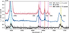 |
Fig. 11. Comparison of SNR 3627-1, SNR 4449-1 and SN 1979C. Solid lines are smoothed spectra, shaded represents the original spectrum. Vertical lines indicate different emission lines; [O III] (cyan), [OI] (magenta), Hα (red), [S II] (pink) and [OII] (yellow). |
SNR 3627-1 is detected with JWST/MIRI, showing a blackbody-like SED with a maxima around 10 μm (Fig. 6). The SNR has a high S/N Chandra counterpart observed in 2008 with a luminosity of 6.5 × 1037 erg/s.
4.4. SNR 3351-5
SNR 3351-5 was detected in all of the linemaps. The spectrum is dominated by a blended Hα+[N II]λ6583 emission, but [O III], very weak [O I] and [S II] are also detected (see Fig. 12). The [O III] doublet is unblended and resolved with a FWHM of 1400 km/s, with a total luminosity of 7 × 1035 erg/s. This source is most reminiscient of a recent SNR detected in M31, identified as a N-rich SNR (Caldwell & Raymond 2023) and therefore we also plot this literature event in Fig. 12. We do not detect the remnant in the JWST observations, but the Chandra observations detect a point source with a luminosity of 4.81 × 1037 erg/s.
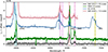 |
Fig. 12. Comparison of SNR 3351-5, SNR 4449-1, SN 1979C and the recently discovered WB92-26 in M31 by Caldwell & Raymond (2023). Solid lines are smoothed spectra, shaded represents the original spectrum. Vertical lines indicate different emission lines; [O III] (cyan), [OI] (magenta), Hα (red), [S II] (pink) and [OII] (yellow). |
4.5. SNR 3627-17
SNR 3627-17 was only detected in the [O III] linemap. It is embedded in a cluster of blue stars. For this source, we removed the stellar continuum using STARLIGHT (Fernandes et al. 2005) and the SEDs of simple stellar populations at different ages with BPASS v2.2.1 (Stanway & Eldridge 2018). The resulting continuum-subtracted spectrum is still noisy, but we detect [O III]λλ4959,5007, [O I]λ6300 and weak Hα and [N II]λ6583 (see Fig. 13). [O III] has the broadest FWHM of all O-rich SNRs in our sample with a width of over 6000 km/s with a total luminosity of 9.1 × 1036 erg/s. We detect the SNR as a bright point-source in both Chandra (see Table A.1 with a total luminosity of 1.35 × 1038 erg/s) and JWST (Fig. 6) observations with a bright red SED; the absolute magnitude with F2100W filter is MAB = −12.18 mag. This remnant and SN 1979C have similar JWST SEDs; there is a small plateau between F1000W and F1130W filters. As with SNR 4303-46, this feature could be indicative of the 14 μm absorption feature inherent to silicate dust.
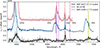 |
Fig. 13. Comparison of SNR 3627-17, SNR 4449-1 and SN 1979C. Solid lines are smoothed spectra, shaded represents the original spectrum. Vertical lines indicate different emission lines; [O III] (cyan), [OI] (magenta), Hα (red), [S II] (pink) and [OII] (yellow). |
4.6. SNR 4303-37
SNR 4303-37 wa detected as a source with a somewhat weak, but broad [O III] emission, with a FWHM of over 2000 km/s for the individual lines in the doublet and a total luminosity of 3.7 × 1036 erg/s, with very weak [OII] and [OI] detections (see Fig. 14). No other line is obvious, but it is reminiscient of SNR 3627-1 and also SNR 4303-20, but without the Hα+[N II]λ6583 and [S II] lines (Figs. 10 and 11). The Chandra data have only a few photons, which is consistent with the diffuse host galaxy flux, giving an upper limit luminosity of 2.1 × 1037 erg/s. The remnant is clearly detected in JWST/MIRI with a blue SED and with an absolute magnitude MAB = −11.99 mag in filter F770W.
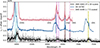 |
Fig. 14. Comparison of SNR 4303-37, SNR 4449-1 and SN 1979C. Solid lines are smoothed spectra, shaded represents the original spectrum. Vertical lines indicate different emission lines; [O III] (cyan), [OI] (magenta), Hα (red), [S II] (pink) and [OII] (yellow). |
4.7. SNR 1566-4
SNR 1566-4 was detected in the [O III] and [S II] linemaps. Only a blueshifted [O III]5007Å is clearly detected with possible blended Hα+[N II]λ6583 and a weak [S II] emission (see Fig. 15). The [O III]λλ4959,5007 lines have FWHM of over 1200 km/s and a total luminosity of 3.7 × 1036 erg/s. It is distinctly different from the other O-rich SNRs in our sample. This could indicate an older age compared to the others, considering the similarity to SNR 0540-69.3 and its reported age of ≈1000 years (Larsson et al. 2021). The SNR is not detected with Chandra or JWST. The X-ray fluxes listed in Table A.1 is based on a single X-ray photon and should be taken as an upper limit.
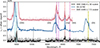 |
Fig. 15. Comparison of SNR 1566-4, SNR 4449-1 and SN 1979C. Solid lines are smoothed spectra, shaded represents the original spectrum. Vertical lines indicate different emission lines; [O III] (cyan), [OI] (magenta), Hα (red), [S II] (pink) and [OII] (yellow). |
5. Discussion
In this article we have presented a new method to search for and identify extragalactic SNRs. We make use of the capabilities of a modern IFU; the fact that SNRs have broad emission lines compared to other emission sources such as photoionized nebulae. In addition, we make use of the compactness of extragalactic SNRs; with the optical quality of MUSE observations the remnants are observed as unresolved point sources. These two considerations allow us to isolate SNRs from the diffuse gas of a host galaxy and other contaminants. We applied our method to a sample of 19 nearby galaxies, the current PHANGS-MUSE catalog. We found a total of 307 SNRs. Of these, seven were found to be O-rich.
The small fraction of O-rich SNRs within the full SNR population indicates that they are observationally rare. They are also only found in 4 of 19 galaxies in our sample. The fraction of O-rich SNRs to all SNRs is consistent with the SNR population in the MW and the Magellanic Clouds. In the literature, out of the roughly 300 SNRs in the MW, only three have been designated to be O-rich. If both of these samples are considered almost complete complete, the rate of O-rich SNRs is only a 1–2% of the SNR population. The Magellanic Clouds host three more previously classified O-rich SNRs and one more has been found in NGC 4449 for a total of seven O-rich SNRs. Our new sample thus doubles the number of known O-rich SNRs. The observed rarity could be due to two reasons:
-
O-rich SNRs are intrinsically rare. This could be because they come from the most massive stars or from a rare progenitor scenario. Other factors affecting rarity include unusually dense CSM and interaction with SN ejecta, or a central compact object interacting with the SN ejecta.
-
O-rich SNRs are only a brief stage in SNR evolution. Age estimates of the known remnants span from a few decades up to a few thousand years. If this stage lasts at most only a few thousand years after the explosion, we will only rarely observe remnants at this stage.
5.1. Observed properties of extragalactic O-rich SNRs
Optical wavelength identification of SNRs has previously been based on empirical line ratios indicating a shocked region. Therefore, their spectra by definition show strong forbidden emission lines of singly-ionised sulphur and nitrogen. O-rich SNRs on the other hand are dominated by emission lines of oxygen with different degrees of ionisation, exemplified by SNR 4449-1. The oxygen lines in some cases are extremely luminous and have high FWHM compared to normal SNRs, upwards of 1038 erg/s and FWHMs exceeding 2000 km/s.
Our sample of O-rich SNRs also have strong detections in both X-rays and the mid-IR. These measurements are extracted from archival observations and hence do not temporally align with the MUSE observations. This also allows us in some cases to give a minimum age to some of the remnants, e.g. SNR 4303-46 was serendipitiously detected by ROSITA already between 1996 and 1998 giving it a current minimum age as 28 years.
5.2. The physical nature of O-rich SNRs
Following the numbers of different SNRs discovered within our sample, we can conclude that O-rich SNRs are rare, but we cannot definitely conclude if this is an intrinsic property or observational effect. Our sample of galaxies in this article also host several historical SNe. We do not detect these SNe in the MUSE dataset, but instead we detect several O-rich SNRs with no known progenitor SN. While the cadence and depth of SN searches within these galaxies have been irregular and sometimes sparse in the hundred years before all-sky surveys, and a more thorough search through old photographic plates should be done in a follow-up study, we can still draw some conclusions on the non-detections. The fact that we do not detect the known SNe with MUSE shows that the SNe ‘normally’ fade away quickly. Even if this ‘O-rich phase’ is a common feature in SNe, it may be typically too faint to be detected. But in some cases we observe bright O-rich SNRs, making them unusual and intrinsically rare. On the other hand, the O-rich phase could be something that happens only to a certain subset of SNe, making them intrinsically rare. Long-term observations of nearby future SNe and a renewed recovery program of historical SNe could shed more light on this issue. If we assume that there is no additional power source accelerating the SN ejecta on long timescales (e.g. at thousands of years post explosion), we can infer that the O-rich SNRs are likely young based on the oxygen line velocities, especially when compared to normal optical SNRs we find outside the MW. The spectral similarity with some historical extragalactic SNe, e.g. SN 1979C, hint that these remnants are indeed middle-aged SNe that have gone undetected.
The high luminosity of O-rich SNRs and their probable longevity requires us to consider the powering methods of the emission. Radioactive nickel and its daughter species are unlikely to be producing the amount of energy we observe in these remnants decades since the explosion. Ejecta-CSM interaction has previously been proposed to be powering the strong emission. Ejecta interacting with dense CSM could cause strong reverse shocks into an O-rich ejecta causing luminous oxygen emission. This scenario would require high mass losses before the explosion with CSM density profiles deviating from r−2 in order to produce a strong reverse shock for decades or hundreds of years. The source of luminosity could also be a compact object injecting extra energy into the ejecta. This could be a magnetar shedding energy from the spin-down or a black hole accreting matter.
Recently, a peculiar type Ib SN, SN 2012au, was observed by Milisavljevic et al. (2018) to exhibit forbidden oxygen emission lines in optical light six years after the explosion. The authors note the possibility of a pulsar or a magnetar embedded in a O-rich ejecta. Similarly, Chevalier & Fransson (1992) had previously showed that a pulsar inside an oxygen-dominated ejecta would produce shells with different ionisations of oxygen. This may explain SN 2012au, as discussed by Milisavljevic et al. (2018), and notably also SNR 3627-1 and SNR 4303-37 in this paper. This may be an indication that SN 2012au and the O-rich SNRs are similar objects. Follow-ups on both the SN and the SNRs should reveal this e.g. if the SN oxygen line keep broadening and the X-ray luminosity stays stable.
Omand & Jerkstrand (2023) has also showed promising numerical models for a magnetar inside ejectas of different compositions. If the compact central object is indeed the main powering mechanism of these SNRs, these models seem to indicate the preference of a highly O-rich ejecta. Otherwise other metals, especially sulfur, would have equal or higher luminosities coming from forbidden emission lines. These lines are also likely not quenched due to high densities, because the critical densities for sulfur lines observable with MUSE are higher than the oxygen lines. Therefore, it is likely that the observed ejecta is O-rich and S-poor. Likewise, this may also give indications of the mass cut for the formation of the compact object. As the proto-neutron star forms, it accretes ∼2 M⊙ of matter. This also includes at least some of the Si-shell of the collapsing star. The Si-shell is also somewhat enriched with sulfur, contrasting to the more S-poor O-shell. It may be that the Si-shell needs to be accreted more or less completely in order to account for the non-detections of sulfur and the strong oxygen emissions.
The cause of the oxygen emission should also ideally explain the strong observed X-ray and mid-IR emissions. Mid-IR implies the precense of warm dust and in the brightest O-rich SNRs in our sample we observe a feature in the SED that can be interpreted as a 14 μm silicon feature. This would still need to be reconciled with the strong X-ray emission. If the X-rays are part of a blackbody emission, this would mean extremely hot gas, which would predicate the destruction of dust. On the other hand, the observed mid-IR excess could be the tail-end of strong synchrotron emission, indicating the presence of a magnetar. If we assume that the X-rays are non-thermal in origin, i.e. arising from a compact object, the presence of dust would be more probable in outer regions, away from the compact object, but the mid-IR excess could still be non-thermal in nature. In any case, detailed and deep observations of these objects with radio and IR (JWST spectra) are needed to better understand their nature.
Considering that these objects resemble both older SNe and specific younger SNRs, they are an important link between SNe and SNRs. The progenitor SN in the case of Cas A was identified as a type IIb, a type of core-collapse SN that initially resembles a H-rich type II, but later evolves into a H-poor type Ib (Filippenko et al. 1993). On the other hand, the SN 1979C used as a comparison in this article was an unusual type II; the SN reached MB ∼ −20, declining linearly with signs of CSM. It was also a bright radio SN. The apparent rarity of O-rich SNRs could also be due to high-mass progenitors. In fact, two O-rich SNRs in our sample are situated in a strongly star-forming regions and SNR 4449-1 is also in a starbursting galaxy. A high mass of the progenitor, implying high mass-losses, may then favour the CSM interaction scenario.
6. Conclusions
In this work, we have reported the discovery of 307 SNRs in the PHANGS-MUSE galaxy catalog. Of these, seven are O-rich SNRs. This doubles the number O-rich SNRs in literature. We also note the similarity of these objects to some long-lasting SNe that exploded a few decades ago. The seven events were found in a search of 19 nearby galaxies and in a total of four host galaxies. This work has thus further outlined the rarity of O-rich SNRs. The methods presented in this paper will be expanded to other nearby galaxies in order to improve our understanding of these objects and to characterise their rarity in the SN/SNR population.
SNRs, and specifically O-rich events, give constraints on the stellar evolutionary pathways that lead to these explosion remnants. In the case of significant CSM interaction, stellar evolution models would need to be able to reproduce the high mass-losses needed to produce the observed results. In compact object powered scenarios the stellar evolution and explosion models need to account for the observed rarity of O-rich SNRs, i.e. why are only some compact central objects related to some specific SNRs? Additional observations and modelling of O-rich SNRs is required to corroborate our findings using optical-wavelength spectroscopy, and further our understanding of the origin and powering mechanism of these SN remnants.
Data availability
Appendix B is available at the CDS via https://cdsarc.cds.unistra.fr/viz-bin/cat/J/A+A/700/A223. Figures of SNR locations in their host galaxies are available at https://doi.org/10.5281/zenodo.15214468. HST and JWST stamps of the O-rich SNR locations are available at https://doi.org/10.5281/zenodo.15214763.
Acknowledgments
This work was funded by ANID, Millennium Science Initiative, ICN12_009. HK was funded by the Research Council of Finland projects 324504, 328898, and 353019. KM acknowledges support from the Japan Society for the Promotion of Science (JSPS) KAKENHI grant (JP20H00174), and by the JSPS Open Partnership Bilateral Joint Research Project (JPJSBP120229923 for Japan-Finland, and JPJSBP120239901 for Japan-Chile). SM acknowledge support from the Research Council of Finland project 350458. Based on observations collected at the European Southern Observatory under ESO programme(s) 1100.B.0651(A-D), 0102.D-0769(A) and/or data obtained from the ESO Science Archive Facility with DOI(s) under https://doi.org/10.18727/archive/47. This research has made use of data obtained from the Chandra Data Archive provided by the Chandra X-ray Center (CXC). This work has made use of data from the European Space Agency (ESA) mission Gaia (https://www.cosmos.esa.int/gaia), processed by the Gaia Data Processing and Analysis Consortium (DPAC, https://www.cosmos.esa.int/web/gaia/dpac/consortium). Funding for the DPAC has been provided by national institutions, in particular the institutions participating in the Gaia Multilateral Agreement.
References
- Anand, G. S., Lee, J. C., Van Dyk, S. D., et al. 2021, MNRAS, 501, 3621 [Google Scholar]
- Bacon, R., Accardo, M., Adjali, L., et al. 2010, in Ground-based and Airborne Instrumentation for Astronomy III, eds. I. S. McLean, S. K. Ramsay, & H. Takami, SPIE Conf. Ser., 7735, 773508 [Google Scholar]
- Balick, B., & Heckman, T. 1978, ApJ, 226, L7 [NASA ADS] [CrossRef] [Google Scholar]
- Bauer, F. E., Dwarkadas, V. V., Brandt, W. N., et al. 2008, ApJ, 688, 1210 [NASA ADS] [CrossRef] [Google Scholar]
- Bertin, E., & Arnouts, S. 1996, A&AS, 117, 393 [NASA ADS] [CrossRef] [EDP Sciences] [Google Scholar]
- Bietenholz, M. F., Bartel, N., Milisavljevic, D., et al. 2010, MNRAS, 409, 1594 [Google Scholar]
- Blair, W. P., & Long, K. S. 1997, ApJS, 108, 261 [NASA ADS] [CrossRef] [Google Scholar]
- Blair, W. P., Kirshner, R. P., & Winkler, P. F., Jr 1983, ApJ, 272, 84 [Google Scholar]
- Blair, W. P., Winkler, P. F., Long, K. S., et al. 2015, ApJ, 800, 118 [Google Scholar]
- Caldwell, N., & Raymond, J. 2023, ArXiv e-prints [arXiv:2308.00754] [Google Scholar]
- Campbell, L. 1926, Popular Astronomy, 34, 402 [Google Scholar]
- Cardelli, J. A., Clayton, G. C., & Mathis, J. S. 1989, ApJ, 345, 245 [Google Scholar]
- Chevalier, R. A., & Fransson, C. 1992, ApJ, 395, 540 [NASA ADS] [CrossRef] [Google Scholar]
- Cid Fernandes, R., Carvalho, M. S., Sanchez, S. F., de Amorim, A. L., & Ruschel-Dutra, D. 2021, ArXiv e-prints [arXiv:2101.12022] [Google Scholar]
- De Looze, I., Barlow, M. J., Swinyard, B. M., et al. 2017, MNRAS, 465, 3309 [NASA ADS] [CrossRef] [Google Scholar]
- de Vaucouleurs, G., de Vaucouleurs, A., Buta, R., Ables, H. D., & Hewitt, A. V. 1981, PASP, 93, 36 [NASA ADS] [CrossRef] [Google Scholar]
- Emsellem, E., Schinnerer, E., Santoro, F., et al. 2022, A&A, 659, A191 [NASA ADS] [CrossRef] [EDP Sciences] [Google Scholar]
- Fernandes, R. C., Mateus, A., Sodré, L., Stasińska, G., & Gomes, J. M. 2005, MNRAS, 358, 363 [CrossRef] [Google Scholar]
- Fernández Arenas, D., Terlevich, E., Terlevich, R., et al. 2018, MNRAS, 474, 1250 [Google Scholar]
- Fesen, R. A., Gerardy, C. L., Filippenko, A. V., et al. 1999, AJ, 117, 725 [NASA ADS] [CrossRef] [Google Scholar]
- Fesen, R. A., Weil, K. E., Cisneros, I. A., Blair, W. P., & Raymond, J. C. 2018, MNRAS, 481, 1786 [Google Scholar]
- Filippenko, A. V., Matheson, T., & Ho, L. C. 1993, ApJ, 415, L103 [NASA ADS] [CrossRef] [Google Scholar]
- Fruscione, A., McDowell, J. C., & Allen, G. E. 2006, in SPIE Conf. Ser., eds. D. R. Silva, & R. E. Doxsey, 6270, 62701V [NASA ADS] [Google Scholar]
- Gaia Collaboration (Prusti, T., et al.) 2016, A&A, 595, A1 [NASA ADS] [CrossRef] [EDP Sciences] [Google Scholar]
- Gaia Collaboration (Vallenari, A., et al.) 2023, A&A, 674, A1 [NASA ADS] [CrossRef] [EDP Sciences] [Google Scholar]
- Gómez-González, V. M. A., Mayya, Y. D., Toalá, J. A., et al. 2021, MNRAS, 500, 2076 [Google Scholar]
- JDADF Developers, Averbukh, J., Bradley, L., et al. 2023, https://doi.org/10.5281/zenodo.10420627 [Google Scholar]
- Krause, O., Birkmann, S. M., Usuda, T., et al. 2008, Science, 320, 1195 [NASA ADS] [CrossRef] [Google Scholar]
- Kuncarayakti, H., Maeda, K., Anderson, J. P., et al. 2016, MNRAS, 458, 2063 [NASA ADS] [CrossRef] [Google Scholar]
- Lacey, C. K., Goss, W. M., & Mizouni, L. K. 2007, AJ, 133, 2156 [Google Scholar]
- Larsson, J., Sollerman, J., Lyman, J. D., et al. 2021, ApJ, 922, 265 [CrossRef] [Google Scholar]
- Lee, J. C., Whitmore, B. C., Thilker, D. A., et al. 2022, ApJS, 258, 10 [NASA ADS] [CrossRef] [Google Scholar]
- Lee, J. C., Sandstrom, K. M., Leroy, A. K., et al. 2023, ApJ, 944, L17 [NASA ADS] [CrossRef] [Google Scholar]
- Leroy, A. K., Schinnerer, E., Hughes, A., et al. 2021, ApJS, 257, 43 [NASA ADS] [CrossRef] [Google Scholar]
- Long, K. S., Blair, W. P., Godfrey, L. E. H., et al. 2012, ApJ, 756, 18 [CrossRef] [Google Scholar]
- Makarenko, E. I., Walch, S., Clarke, S. D., et al. 2023, MNRAS, 523, 1421 [NASA ADS] [CrossRef] [Google Scholar]
- Martínez-Rodríguez, H., Galbany, L., Badenes, C., et al. 2024, ApJ, 963, 125 [Google Scholar]
- Matonick, D. M., & Fesen, R. A. 1997, ApJS, 112, 49 [NASA ADS] [CrossRef] [Google Scholar]
- Meaburn, J., Redman, M. P., Boumis, P., & Harvey, E. 2010, MNRAS, 408, 1249 [Google Scholar]
- Micelotta, E. R., Matsuura, M., & Sarangi, A. 2018, Space Sci. Rev., 214, 53 [NASA ADS] [CrossRef] [Google Scholar]
- Milisavljevic, D., & Fesen, R. A. 2008, ApJ, 677, 306 [Google Scholar]
- Milisavljevic, D., Fesen, R. A., Chevalier, R. A., et al. 2012, ApJ, 751, 25 [NASA ADS] [CrossRef] [Google Scholar]
- Milisavljevic, D., Patnaude, D. J., Chevalier, R. A., et al. 2018, ApJ, 864, L36 [NASA ADS] [CrossRef] [Google Scholar]
- Niculescu-Duvaz, M., Barlow, M. J., Bevan, A., et al. 2022, MNRAS, 515, 4302 [NASA ADS] [CrossRef] [Google Scholar]
- Omand, C. M. B., & Jerkstrand, A. 2023, A&A, 673, A107 [NASA ADS] [CrossRef] [EDP Sciences] [Google Scholar]
- Patnaude, D. J., & Fesen, R. A. 2003, ApJ, 587, 221 [Google Scholar]
- Patnaude, D. J., Loeb, A., & Jones, C. 2011, New Astron., 16, 187 [Google Scholar]
- Schenck, A., Park, S., Burrows, D. N., et al. 2014, ApJ, 791, 50 [Google Scholar]
- Schönberner, D., Balick, B., & Jacob, R. 2018, A&A, 609, A126 [NASA ADS] [CrossRef] [EDP Sciences] [Google Scholar]
- Seaquist, E. R., & Bignell, R. C. 1978, ApJ, 226, L5 [Google Scholar]
- Smith, R. C., Kirshner, R. P., Blair, W. P., Long, K. S., & Winkler, P. F. 1993, ApJ, 407, 564 [Google Scholar]
- Stanway, E. R., & Eldridge, J. J. 2018, MNRAS, 479, 75 [NASA ADS] [CrossRef] [Google Scholar]
- Tinyanont, S., Kasliwal, M. M., Fox, O. D., et al. 2016, ApJ, 833, 231 [NASA ADS] [CrossRef] [Google Scholar]
- Tschöke, D., Hensler, G., & Junkes, N. 2000, A&A, 360, 447 [NASA ADS] [Google Scholar]
- Vogt, F., & Dopita, M. A. 2010, Astrophys. Space Sci., 331, 521 [Google Scholar]
- Weiler, K. W., van der Hulst, J. M., Sramek, R. A., & Panagia, N. 1981, ApJ, 243, L151 [Google Scholar]
- Wesson, R., Bevan, A. M., Barlow, M. J., et al. 2023, MNRAS, submitted [arXiv:2308.09028] [Google Scholar]
Appendix A: Chandra and JWST photometry
This appendix presents the Chandra X-ray observations and JWST photometry.
Measurements of Chandra X-ray fluxes and luminosities based on the absorbed model flux. Luminosity range within the 90% interval is presented in the parentheses. We assume a power law model with a power law index of 2. The last two source have very few photons, 4303-41 has three and 1566-5 only has one. Qualitatively these are likely incidental and the fluxes are just an absolute upper limit. Distances to the host galaxies are adopted from Anand et al. (2021).
Archival JWST observations of sources. All observations are part of the PHANGS-JWST program. The measurements were done with Jdaviz, using an aperture with a radius of four pixels. Background emission was estimated with an annular ring with and inner radius of four pixels and width of two pixels. For the upper limits we use the fluxes obtained from a similar aperture with no background subtraction.
Appendix B: Tables of SNRs
In this appendix we present all of SNRs discovered in our survey of PHANGS-MUSE galaxies. The selected lines are used in Fig. 3 as a diagnostic tool to identify them as SNRs. The tables are available in electronic form at the CDS.
Appendix C: Space telescope observations used
This appendix lists all of the data used from HST, JWST and Chandra. The tables list all filters used, observation dates, exposure times, proposal ID of the programs, their PI’s and the instruments used.
The observations from HST, JWST, and Chandra used in this article for NGC 4303. The tables list the filter and instrument used, observation date, total exposure time, Proposal ID and the PI of the proposal they originate from.
Same as Table C.1 for NGC 3627.
Same as Table C.1 for NGC 3351.
Same as Table C.1 for NGC 1566.
Appendix D: O-rich SNR emission line profile comparisons
The appendix presents the velocity space comparisons of oxygen emission lines of six O-rich SNRs. SNR 4303-46 is presented in the main text, Fig. 9
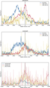 |
Fig. D.1. [O III]λλ4959,5007 emission complex in velocity space centered around 5006.8Å (top) and same for [O I]λλ6300,6364 centered around 6300Å (second panel). The visible-light oxygen lines of SNR 4303-20 in velocity space centered on 5006.8 Å, 6300.3 Å and 7319.9 Å (third panel). The spectra are normalized arbitrarily to have similar peak intensities. |
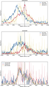 |
Fig. D.2. [O III]λλ4959,5007 emission complex in velocity space centered around 5006.8Å (top) and same for [O I]λλ6300,6364 centered around 6300Å (second panel). The visible-light oxygen lines of SNR 3627-1 in velocity space centered on 5006.8 Å, 6300.3 Å and 7319.9 Å (third panel). The spectra are normalized arbitrarily to have similar peak intensities. |
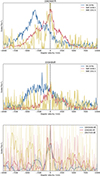 |
Fig. D.3. [O III]λλ4959,5007 emission complex in velocity space centered around 5006.8Å (top) and same for [O I]λλ6300,6364 centered around 6300Å (second panel). The visible-light oxygen lines of SNR 3351-5 in velocity space centered on 5006.8 Å, 6300.3 Å and 7319.9 Å (third panel). The spectra are normalized arbitrarily to have similar peak intensities. |
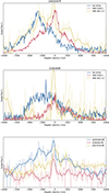 |
Fig. D.4. [O III]λλ4959,5007 emission complex in velocity space centered around 5006.8Å (top) and same for [O I]λλ6300,6364 centered around 6300Å (second panel). The visible-light oxygen lines of SNR 3627-17 in velocity space centered on 5006.8 Å, 6300.3 Å and 7319.9 Å (third panel). The spectra are normalized arbitrarily to have similar peak intensities. |
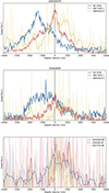 |
Fig. D.5. [O III]λλ4959,5007 emission complex in velocity space centered around 5006.8Å (top) and same for [O I]λλ6300,6364 centered around 6300Å (second panel). The visible-light oxygen lines of SNR 4303-37 in velocity space centered on 5006.8 Å, 6300.3 Å and 7319.9 Å (third panel). The spectra are normalized arbitrarily to have similar peak intensities. |
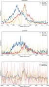 |
Fig. D.6. [O III]λλ4959,5007 emission complex in velocity space centered around 5006.8Å (top) and same for [O I]λλ6300,6364 centered around 6300Å (second panel). The visible-light oxygen lines of SNR 1566-4 in velocity space centered on 5006.8 Å, 6300.3 Å and 7319.9 Å (third panel). The spectra are normalized arbitrarily to have similar peak intensities. |
All Tables
Measurements of Chandra X-ray fluxes and luminosities based on the absorbed model flux. Luminosity range within the 90% interval is presented in the parentheses. We assume a power law model with a power law index of 2. The last two source have very few photons, 4303-41 has three and 1566-5 only has one. Qualitatively these are likely incidental and the fluxes are just an absolute upper limit. Distances to the host galaxies are adopted from Anand et al. (2021).
Archival JWST observations of sources. All observations are part of the PHANGS-JWST program. The measurements were done with Jdaviz, using an aperture with a radius of four pixels. Background emission was estimated with an annular ring with and inner radius of four pixels and width of two pixels. For the upper limits we use the fluxes obtained from a similar aperture with no background subtraction.
The observations from HST, JWST, and Chandra used in this article for NGC 4303. The tables list the filter and instrument used, observation date, total exposure time, Proposal ID and the PI of the proposal they originate from.
All Figures
|
Fig. 1. Colour image of M61 compiled from three narrow-line maps used in this survey; red, green and blue colours correspond to [SII], Hα and [OIII], respectively. The background image is the collapsed cube of the MUSE observation. White circles and numbers are the SNRs in the galaxy confirmed by this survey. Magenta stars indicate the locations of previously observed SNe in the field of view. Gold stars show the locations of the three O-rich SNRs in the galaxy. Corresponding stamps of the other host galaxies are available here. |
| In the text | |
|
Fig. 2. Comparison of [SII]λλ6717,6731 emission lines from a SNR and an HII region, scaled to similar peak fluxes. The area bounded by black vertical lines (black arrows) is extracted and continuum subtracted. The difference in flux extracted between the two sources is apparent. |
| In the text | |
|
Fig. 3. Our sample of broadened emission lines that have detectable Hα, [N II]λ6583 and [S II]λλ6717,6731 emission lines and that we identify as SNRs. Colour of the points represent the FWHM of the [N II]λ6583 with the instrumental broadening removed. The different regions in the figure have been adopted from Meaburn et al. 2010. Most of our sample aligns with the SNR region with log(Hα/[S II]) < 0.5. |
| In the text | |
|
Fig. 4. Optical wavelength spectra of all seven O-rich SNRs discovered by our work. We addditionally display the spectra of three SNe at 15–40 years post explosion, SNR 4449-1, and also include a spectrum of SNR 0540-69.3, an old O-rich SNR in the LMC. |
| In the text | |
|
Fig. 5. X-ray image of NGC 4303 obtained with Chandra, observed in August 2001. None of the historical SNe have an associated source in X-ray, but both SNR 4303-46 and SNR 4303-20 are detected. SNR 4303-20 is considerably dimmer compared to SNR 4303-46, while SNR 4303-37 has very faint detection. |
| In the text | |
|
Fig. 6. JWST observations of the new O-rich SNRs compared to SN 1979C with JWST and SN 1995N from Wesson et al. (2023). |
| In the text | |
|
Fig. 7. Image of SN 1926A observed on May 11th 1926. We calibrated the coordinate solution based on stars observed by Gaia (blue circles). The SN location is identified (green circle) with the nearby SNR 4303-46 (red circle). The arrow length of the compass is 30″ in the inset. |
| In the text | |
|
Fig. 8. Comparison of SNR 4303-46, SNR 4449-1 and SN 1979C. Solid lines are smoothed spectra, shaded represents the original spectrum. Vertical lines indicate different emission lines; [O III] (cyan), [O I] (magenta), Hα (red), [S II] (pink) and [O II] (yellow). |
| In the text | |
|
Fig. 9. [O III]λλ4959,5007 emission complex in velocity space centered around 5006.8 Å (top) and same for [O I]λλ6300,6364 centered around 6300 Å (second panel). The oxygen lines of SN1979C with the addition of [O II]λλ7320,7330 centered at 7320 Å (third panel) and the same lines for SNR 4303-5 (bottom panel). The spectra are normalized arbitrarily to have similar peak intensities. Corresponding figures to other O-rich SNRs are presented in Appendix D. |
| In the text | |
|
Fig. 10. Comparison of SNR 4303-20, SNR 4449-1 and SN 1979C. Solid lines are smoothed spectra, shaded represents the original spectrum. Vertical lines indicate different emission lines; [O III] (cyan), [OI] (magenta), Hα (red), [S II] (pink) and [OII] (yellow). |
| In the text | |
|
Fig. 11. Comparison of SNR 3627-1, SNR 4449-1 and SN 1979C. Solid lines are smoothed spectra, shaded represents the original spectrum. Vertical lines indicate different emission lines; [O III] (cyan), [OI] (magenta), Hα (red), [S II] (pink) and [OII] (yellow). |
| In the text | |
|
Fig. 12. Comparison of SNR 3351-5, SNR 4449-1, SN 1979C and the recently discovered WB92-26 in M31 by Caldwell & Raymond (2023). Solid lines are smoothed spectra, shaded represents the original spectrum. Vertical lines indicate different emission lines; [O III] (cyan), [OI] (magenta), Hα (red), [S II] (pink) and [OII] (yellow). |
| In the text | |
|
Fig. 13. Comparison of SNR 3627-17, SNR 4449-1 and SN 1979C. Solid lines are smoothed spectra, shaded represents the original spectrum. Vertical lines indicate different emission lines; [O III] (cyan), [OI] (magenta), Hα (red), [S II] (pink) and [OII] (yellow). |
| In the text | |
|
Fig. 14. Comparison of SNR 4303-37, SNR 4449-1 and SN 1979C. Solid lines are smoothed spectra, shaded represents the original spectrum. Vertical lines indicate different emission lines; [O III] (cyan), [OI] (magenta), Hα (red), [S II] (pink) and [OII] (yellow). |
| In the text | |
|
Fig. 15. Comparison of SNR 1566-4, SNR 4449-1 and SN 1979C. Solid lines are smoothed spectra, shaded represents the original spectrum. Vertical lines indicate different emission lines; [O III] (cyan), [OI] (magenta), Hα (red), [S II] (pink) and [OII] (yellow). |
| In the text | |
|
Fig. D.1. [O III]λλ4959,5007 emission complex in velocity space centered around 5006.8Å (top) and same for [O I]λλ6300,6364 centered around 6300Å (second panel). The visible-light oxygen lines of SNR 4303-20 in velocity space centered on 5006.8 Å, 6300.3 Å and 7319.9 Å (third panel). The spectra are normalized arbitrarily to have similar peak intensities. |
| In the text | |
|
Fig. D.2. [O III]λλ4959,5007 emission complex in velocity space centered around 5006.8Å (top) and same for [O I]λλ6300,6364 centered around 6300Å (second panel). The visible-light oxygen lines of SNR 3627-1 in velocity space centered on 5006.8 Å, 6300.3 Å and 7319.9 Å (third panel). The spectra are normalized arbitrarily to have similar peak intensities. |
| In the text | |
|
Fig. D.3. [O III]λλ4959,5007 emission complex in velocity space centered around 5006.8Å (top) and same for [O I]λλ6300,6364 centered around 6300Å (second panel). The visible-light oxygen lines of SNR 3351-5 in velocity space centered on 5006.8 Å, 6300.3 Å and 7319.9 Å (third panel). The spectra are normalized arbitrarily to have similar peak intensities. |
| In the text | |
|
Fig. D.4. [O III]λλ4959,5007 emission complex in velocity space centered around 5006.8Å (top) and same for [O I]λλ6300,6364 centered around 6300Å (second panel). The visible-light oxygen lines of SNR 3627-17 in velocity space centered on 5006.8 Å, 6300.3 Å and 7319.9 Å (third panel). The spectra are normalized arbitrarily to have similar peak intensities. |
| In the text | |
|
Fig. D.5. [O III]λλ4959,5007 emission complex in velocity space centered around 5006.8Å (top) and same for [O I]λλ6300,6364 centered around 6300Å (second panel). The visible-light oxygen lines of SNR 4303-37 in velocity space centered on 5006.8 Å, 6300.3 Å and 7319.9 Å (third panel). The spectra are normalized arbitrarily to have similar peak intensities. |
| In the text | |
|
Fig. D.6. [O III]λλ4959,5007 emission complex in velocity space centered around 5006.8Å (top) and same for [O I]λλ6300,6364 centered around 6300Å (second panel). The visible-light oxygen lines of SNR 1566-4 in velocity space centered on 5006.8 Å, 6300.3 Å and 7319.9 Å (third panel). The spectra are normalized arbitrarily to have similar peak intensities. |
| In the text | |
Current usage metrics show cumulative count of Article Views (full-text article views including HTML views, PDF and ePub downloads, according to the available data) and Abstracts Views on Vision4Press platform.
Data correspond to usage on the plateform after 2015. The current usage metrics is available 48-96 hours after online publication and is updated daily on week days.
Initial download of the metrics may take a while.