| Issue |
A&A
Volume 700, August 2025
|
|
|---|---|---|
| Article Number | A228 | |
| Number of page(s) | 22 | |
| Section | Extragalactic astronomy | |
| DOI | https://doi.org/10.1051/0004-6361/202451328 | |
| Published online | 28 August 2025 | |
The physical properties of candidate neutrino-emitter blazars
1
Julius-Maximilians-Universität Würzburg, Fakultät für Physik und Astronomie, Institut für Theoretische Physik und Astrophysik, Lehrstuhl für Astronomie, Emil-Fischer-Str. 31, D-97074
Würzburg, Germany
2
Deutsches Elektronen-Synchrotron DESY, Platanenallee 6, 15738
Zeuthen, Germany
3
Université Paris Cité, CNRS, Astroparticule et Cosmologie, F-75013
Paris, France
⋆ Corresponding author: This email address is being protected from spambots. You need JavaScript enabled to view it.
Received:
1
July
2024
Accepted:
4
July
2025
Abstract
Context. The processes governing the production of astrophysical high-energy neutrinos are still a matter of debate, and the sources that originate them remain an open question. Among the putative emitters, active galactic nuclei (AGN) have gained increasing attention in recent years. Blazars, in particular, stand out due to their capability of accelerating particles in environments with external radiation fields. Recent observations suggest that they may play a role in the production of high-energy neutrinos detected by the IceCube observatory.
Aims. We studied the physical properties of a subsample of 52 blazars, that have been proposed as candidate neutrino emitters, based on a positional cross-correlation statistical analysis between IceCube hotspots and the Fifth Edition of the Roma BZCat catalog. We provide a first characterization of their central engines and inner physical nature, which may help to explore the potential link with neutrino production.
Methods. This study carries out an analysis of the optical spectroscopic properties of a sample of 52 candidate neutrino-emitter blazars, to infer their accretion regime. It is complemented by data at the radio and γ-ray frequencies, which carry the information about the intrinsic power of the relativistic jet. We compared the properties of the sample of candidate neutrino-emitter blazars to other blazar samples from the literature. To this end, we performed statistical tests and also explored, through simulations, the applicability of methods that include limits (censored data) on the quantities of our interest.
Results. Overall, the sample of candidate neutrino-emitter blazars displays properties compatible with those of the reference samples. We observe a mild tendency to prefer objects with intense radiation fields (which are typical of radiatively efficient accretors), and high radio power, such as high-excitation radio galaxies (HERGs). Among the blazars in our sample, 24 are detected in γ-rays; they cover various ranges of γ-ray luminosities, compatible with the overall population. Additionally, we show that the statistical tests commonly used in the literature need to be used with caution, as they are highly sensitive to the amount of censored data and the sample size.
Key words: black hole physics / line: identification / neutrinos / galaxies: active / gamma rays: galaxies / radio continuum: galaxies
Now at Departament d’Astronomia i Astrofísica, Universitat de València, C/ Dr. Moliner, 50, 46100, Burjassot, València, Spain.
© The Authors 2025
 Open Access article, published by EDP Sciences, under the terms of the Creative Commons Attribution License (https://creativecommons.org/licenses/by/4.0), which permits unrestricted use, distribution, and reproduction in any medium, provided the original work is properly cited.
This article is published in open access under the Subscribe to Open model. This email address is being protected from spambots. You need JavaScript enabled to view it. to support open access publication.
1. Introduction
The IceCube Neutrino Observatory at the South Pole is the most sensitive detector currently operating to investigate the origin of astrophysical high-energy neutrinos. Neutrinos are unique messengers that allow us to study our Universe because they travel long cosmological distances almost unimpeded and carry information about the location of their sources. In 2013, the IceCube Collaboration reported the detection of a diffuse high-energy neutrino flux consistent with an astrophysical origin in the ≳100 TeV to 10 PeV energy range (IceCube Collaboration 2013; Aartsen et al. 2016). High-energy neutrinos are created in processes that involve the interaction of cosmic rays with matter or radiation. Therefore, they represent the “smoking gun” signature of cosmic-ray sources. The astrophysical sources that originate them remain largely uncertain.
Among the most luminous and persistent sources in the universe are active galactic nuclei (AGN), which are highly powerful astrophysical objects able to emit throughout the whole electromagnetic spectrum, from radio frequencies up to the γ-ray band. According to theoretical models (Blandford & Payne 1982), they are powered by accretion onto a central supermassive black hole (SMBH), and have masses that range from millions to billions of solar masses. These can be spinning Kerr BHs that release a fraction of their kinetic energy via a large-scale magnetic field (Blandford & Znajek 1977). Blazars are a subclass of AGN, characterized by ultra-relativistic jets that point toward the observer’s line of sight. The spectral energy distribution (SED) of blazars typically displays a double-humped shape, with a low-energy peak typically in the infrared (IR)–X-rays, and the high-energy peak in the hard X-rays and/or γ-rays (Fossati et al. 1998; Fan et al. 2016). The first peak is explained by synchrotron radiation emitted by the population of accelerated electrons in the relativistic jet, while, in leptonic models, the second peak is attributed to inverse Compton radiation. Although this framework has been effective in describing the multiwavelength emission of the majority of blazars, it may be reasonable to expect that hadrons are present alongside leptons. The possibility of relativistic jets being able to accelerate hadrons requires exploring lepto-hadronic and/or hadronic scenarios. Hadronic frameworks, although less favored compared to the leptonic scenario for many blazars, open up the perspective of exploring the link between blazars and neutrinos.
In blazar jets within the hadronic scenarios, neutrinos can be the result of either proton-proton (p-p) or proton-photon (p-γ) interactions (for a review, see Cerruti 2020). In the former case, a proton of higher energy interacts with a less energetic one, producing pions and neutrinos as a result. In the latter case, protons of the jet interact with the lower-energy radiation fields, either internal or external, through photo-meson (or photo-pion) interaction or Bethe-Heitler pair production (Mannheim 1993; Böttcher et al. 2013; Dermer et al. 2014). This leads to muons and neutrinos as by-products.
For this work we were mostly interested in p-γ interactions as the combination of efficient particle acceleration and external radiation fields can foster neutrino production in blazars (Dermer et al. 2014). Blazars can host external radiation fields, i.e., from the accretion disk and the re-processed disk emission by the broad and narrow line region, and the dusty torus through external Compton (EC). The photo-pion production efficiency, i.e., the physics governing the production of neutrinos, is tightly linked to the different modes of accretion. These are primarily traced by emission in the optical–IR band.
Studies in the literature suggest that blazars may originate neutrinos, contributing to the observed high-energy diffuse astrophysical neutrino flux (Mannheim 1993; Dermer et al. 2014; Aartsen et al. 2017a; Abbasi et al. 2022). In 2017, the γ-ray blazar TXS 0506+056was associated with a candidate muon-neutrino event, with a chance association at the 3σ level (IceCube Collaboration 2018). More recent works have provided evidence for a correlation between a subset of 52 blazars and IceCube neutrino data, suggesting that blazars may be the first population of extragalactic high-energy neutrino emitters (Buson et al. 2022a, hereafter PAPER I; Buson et al. 2023, hereafer PAPER II; see also Buson et al. 2022b and Bellenghi et al. 2023).
While the statistical significance indicates that the correlation between the two samples is unlikely to arise by chance, it should not be mistaken for the probability of individual neutrino–blazar associations. It is improbable that all 52 candidates are genuinely connected to the neutrinos. Among them, one should expect a non-negligible number of spurious associations by chance (simply by Poisson probability). Assessing the genuineness of the individual associations remains challenging, especially given the proprietary nature of the IceCube data and analysis tools (see also Barbano et al. (2023), Lincetto et al., in prep.).
Bearing this in mind, in this paper we explore the physical properties of the full set of 52 candidate neutrino-emitters − which may include a non-negligible number of spurious associations − and compare them to those of the general blazar population. Based on the energy of the IceCube neutrino dataset, these candidate neutrino emitters may be capable of accelerating protons to energies up to the petaelectronvolt (PeV) range. Therefore, we refer to them as candidate “PeVatron blazars”.
We provide a first multiwavelength characterization of the intrinsic physical properties of the 52 candidate neutrino-emitter blazars, exploiting optical spectroscopy complemented by radio and γ-ray information from the literature.
As the production of neutrinos depends on the object’s accretion regime and radiation field properties (within lepto-hadronic frameworks), studying the behavior at different frequencies probes various aspects of the underlying physics (see, e.g., Fichet de Clairfontaine et al. 2023; Sanchez Zaballa et al. 2025; Pfeiffer 2022, 2024). Section 2 introduces the blazar classification scheme based on the intrinsic physical properties used in this work. Section 3 addresses the blazar sample. In Sects. 4 and 5, we describe the employed dataset and the procedure that we adopted in the analysis. Then, in Sect. 6 we present our findings about the properties of the sources and discuss the results in the broader context of the overall blazar population. This work assumes a flat ΛCDM cosmology with  , Ω0 = 0.29 and ΩΛ = 0.71.
2. The classification of blazars
2.1. The traditional classification scheme
In the AGN unification model (Urry & Padovani 1995; Urry 2004), jetted AGN are traditionally classified into BL Lacertae (BL Lacs, BLLs) and flat spectrum radio quasars (FSRQs) based on the strength of the lines in the optical spectrum. The historical dividing criterion between the two classes is set by the rest-frame equivalent width (EW) of the emission lines. The latter measures the observed line strength, by definition, being the integrated line flux with respect to the underlying continuum emission. EW < 5 Å defines BLLs and EW > 5 Å FSRQs. Phenomena such as variations in the jet power and the orientation with respect to the observer’s line of sight mean that this purely observational classification is not always reliable and/or consistent over time. Smaller or larger EW values could be due to beaming effects and variability in the nonthermal continuum, without necessarily indicating intrinsically lower or higher line luminosity (Ghisellini et al. 2011b).
Attempts in the literature to follow the observation-driven classification scheme required to coin new nomenclature for subsets of blazars that may show ambiguous properties (e.g., properties of both the FSRQs and BL Lacs classes). This is, for example, the case of “blue flat spectrum radio quasars” (Ghisellini et al. 2012), also known as “high-power high-synchrotron-peak blazars”, also known as “masquerading BL Lacs” (Padovani et al. 2012, 2019). Blue FSRQs (masquerading BLLs) appear as BL Lacs based on the featureless optical spectrum and high synchrotron peak. However, they are proposed to be intrinsically FSRQs with their broad emission lines swamped by the jet’s powerful synchrotron emission.
Similarly, objects that have been observed to transition from BL Lac to FSRQ, and/or vice versa, following the appearance or disappearance of optical lines, have been dubbed as “changing-look blazars” (Vermeulen et al. 1995; Ghisellini et al. 2011b; Ruan et al. 2014; Peña-Herazo et al. 2021, Azzollini et al., in prep.). It remains unclear whether the observed changes correspond to intrinsic physical variations. These transition objects may be sources with highly beamed jets, and radiatively efficient accretion, in which sudden variations in the interplay between the thermal and the nonthermal emission may affect the appearance of the optical spectra, leading to the (apparent) variability of the emission lines over time.
As the nature of AGN is closely related to the accretion of matter onto the central SMBH, a physically driven distinction is based on the different accretion modes. The latter characterizes the AGN activity and the main energy mechanism governing their evolution (Best & Heckman 2012; Heckman & Best 2014). On the one hand, when the dominant energetic output is in the form of electromagnetic radiation, we are dealing with “radiative-mode” AGN (i.e., high-excitation radio galaxies; hereafter HERGs), which show the traditional internal structure of an SMBH surrounded by a geometrically thin, optically thick accretion disk (AD). A hot corona surrounds the accretion disk, which scatters the photons of the disk to X-ray energies. The SMBH and AD are surrounded by a dusty torus (DT) of obscuring molecular gas on larger scales. In this schematic view, the luminous ultraviolet (UV) radiation from the AD illuminates the broad line region (BLR), which is located close to it, and the narrow line region (NLR) further out. The radiatively efficient accretion occurs through cold gas piling up on the core of the AGN, and this leads to the establishment of a stable disk. Objects of this class are generally associated with star formation in the host galaxy. The bulk of the energy output is emitted through radiation, however, they can often show traces of radio jets that extend for tens or hundreds of kiloparsecs. On the other hand, in “jet-mode” AGN (i.e., low-excitation radio galaxies; hereafter LERGs), the radiative emission is usually less powerful, and the energy output is dominated by bulk kinetic energy transported in powerful jets. For this second category, it is suggested that in place of the thin accretion disk, there is a geometrically thick advection-dominated accretion flow (ADAF). These radiatively inefficient accretors are thought to be fuelled via hot gas (“hot-mode” accretion) subject to the Bondi mechanism (Bondi 1952). The distribution of observed radio energies of the two classes covers a broad range. However, HERGs are found to dominate at high radio luminosity, while LERG objects dominate at lower values. Adopting the radio power at 1.4 GHz, the dividing threshold falls at P1.4GHz ∼ 1026 W ⋅ Hz−1 (Best & Heckman 2012).
It has long been argued that the different accretion modes could originate a dichotomy in jetted AGN (e.g., Ghisellini & Celotti 2001; Maraschi & Tavecchio 2003; Ghisellini et al. 2009; Giommi et al. 2012; Antonucci 2012). Ghisellini et al. (2011b) proposed a classification scheme for blazars based on the accretion efficiency: FSRQ objects, where the presence of broad optical emission lines implies intense radiation fields, are related to efficient radiative-mode sources (i.e., HERGs), while BLL objects, which are characterized by the lack of prominent emission lines, correspond to inefficient hot-mode accretors (LERGs). The proposed discriminating parameter is the luminosity of the BLR in Eddington units with the threshold reference LBLR/LEdd ≳ 5 × 10⁻⁴. The γ-ray luminosity in Eddington units is also a good tracer of both the accretion efficiency (in the case of intense radiation fields) and the jet power (in all cases), and the dividing line has been proposed at Lγ/LEdd ≳ 0.1 in this case. The distinction places FSRQs above these thresholds, whereas BL Lacs with the ADAF are found below (Ghisellini et al. 2010, 2011b; Sbarrato et al. 2012, 2014). While there is likely continuity between the two extremes rather than a clear-cut separation between the two classes, this distinction is helpful for depicting the underlying physics. The LBLR/LEdd and Lγ/LEdd are proxies for the accretion power and take into account the differences in black hole mass due to the normalization factor being the Eddington luminosity. Within this physically driven scheme, the LERG–HERG discrimination brings less ambiguity in transitional objects, naturally describing blue FSRQs (masquerading BL Lacs) as HERG objects based on their physical properties. Blue FSRQs encompass sources which are intrinsically FSRQ whose emission lines are washed out by a bright, Doppler-boosted jet continuum, unlike “true” BL Lacs, which are intrinsically weak-line objects (see Ghisellini et al. 2011b; Padovani et al. 2022b). Similarly, for changing-look blazars, the apparent line luminosity variations are due to observational biases, while the underlying physics of the objects remains the same. The boundary between the two regimes is only loosely defined, the quantities have rather large errors and the models involved are rather simplistic. As a consequence, we caution that the HERG–LERG distinction is still expected to suffer from observational limitations and the transition between the two classes is expected to be gradual. In the context of potential neutrino emission, the interesting aspect is not the precise classification of an object, but rather the possible presence or absence of radiation fields external to the jet. HERG-like objects benefit from multiple external radiation fields, including the accretion disk, photons reprocessed in the BLR, and emission from the dusty torus. These additional photon targets for protons may foster neutrino production compared to LERGs.
2.2. This work’s taxonomy
In this work, we departed from the historical observation-driven classifications of blazars and hereafter embraced the physically driven view of HERGs and LERGs, based on the accretion regime and high- and low-excitation properties. In blazars, intense radiation fields are traced by the spectral emission lines produced in the BLR and NLR. The radio power P1.4 GHz and the γ-ray luminosity Lγ carry the information about the intrinsic power of the relativistic jet. In the simplified view that we adopted, the distinction between the two classes may be primarily traced by the following properties,
-
The Eddington-scaled accretion rate to the central black hole mass, which sets the separation between radiatively efficient and radiatively inefficient accretion modes; HERGs are then defined by LBLR/LEdd ≳ 5 × 10⁻⁴;
-
The γ-ray Eddington ratio, where higher values, Lγ/LEdd ≳ 0.1, are typically displayed by HERGs compared to LERGs;
-
The radio power, which informs about the jet power, where HERGs have typically higher power, P1.4 GHz ≳ 1026 W ⋅ Hz−1 compared to LERGs.
This classification based on the radiative efficiency of accretion, the intensity of radiation fields, and the radio and γ-ray power, is similar to the one used in previous works (Ghisellini et al. 2010; Giommi et al. 2012; Best & Heckman 2012; Heckman & Best 2014; Padovani et al. 2022b) for discriminating HERGs–LERGs following physically driven markers. However, the boundaries between HERGs and LERGs are not sharply defined, and the transition between these categories is likely to be gradual.
3. The blazar sample
3.1. Target sample
In our previous studies, we explored the potential link between blazars and high-energy neutrinos (Buson et al. 2022a, 2023, PAPER I and PAPER II). To mitigate biased classifications affecting the selection of our sample, we used the fifth data release of the Roma BZCat catalog (5BZCat, see Massaro et al. 2014). This compilation of 3561 sources does not rely on selections in specific wavelengths or survey strategies and has already proved to be effective in unraveling unexpected discoveries (e.g., the “WISE blazar strip”, Massaro et al. 2011). The 5BZCat catalog is not complete as the sky coverage of the surveys used to build it is not uniform, however, it is rather “pure”. For each object of the 5BZCat, an optical spectrum is available and individually inspected to ensure the blazar nature. In 5BZCat, objects are further taxonomically categorized according to the historical classification based on optical spectroscopy; for example, BL Lacs are indicated as “BZB”, FSRQs as “BZQ”, and blazars of uncertain type as “BZU”. In addition, blazars displaying an optical spectrum dominated by the contribution of the host galaxy are referred to as “BZG”.
In PAPER I and PAPER II, 5BZCat sources were positionally cross-matched with all-sky high-level neutrino data, in the form of the skymaps publicly released by the IceCube Collaboration. For the southern celestial hemisphere (−85° < δ < −5°), the analysis was based on the 7 years data recorded between 2008–2015 (Aartsen et al. 2017b; Buson et al. 2022a). For the northern celestial hemisphere (−3° ≤δ ≤ 81°), the analysis exploited the most recent neutrino sky-map released in Abbasi et al. (2022), that encompasses 9 years of neutrino observations (2011–2020, Buson et al. 2023).
The analysis focused on sky locations displaying the highest discrepancy from background expectations, i.e., “hotspots”, as the most promising locations of putative neutrino cosmic sources. The hotspots are identified by the highest L values, defined as the negative logarithm of the provided local pvalue in the IceCube maps, L = −log(pvalue). The positional cross-correlation analysis was performed separately for the southern and northern celestial hemispheres. The analysis resulted in a post-trial chance probability 2 × 10⁻⁶(4.5σ) for the southern dataset and 6.79 × 10⁻³(2.47σ) for the northern dataset, suggesting that the correlation between the blazar and neutrino samples is unlikely to arise by chance. The investigative approach pinpointed a subset of 52 blazars, ten hosted in the southern and 42 in the northern celestial hemisphere, as promising candidates for the production of IceCube neutrinos. As anticipated in Sect. 1, the sample includes a non-negligible number of spurious associations. The reliability of the individual blazar-neutrino associations is difficult to access and will be addressed in a forthcoming work.
Table A.1 lists the 5BZCat sources proposed as associated with neutrino hotspots. The first four columns report the name, coordinates, and L value of the neutrino hotspots (for more details see PAPER I, PAPER II). The following two columns list the associated 5BZCat blazars with the corresponding redshift information. For the redshift, we report the values collected by inspecting the most recent literature and cross-checking with the optical spectrum available from this work. The seventh column reports the blazar Fermi-LAT counterpart from the Third Data Release of the Fourth Fermi Large Area Telescope (LAT) AGN Catalog (4LAC-DR3, Ajello et al. 2022). Finally, the last column lists the reference to the optical spectrum used for the object. Eight blazars of our sample of interest have already been included in other works as promising candidates for the production of high-energy IceCube neutrinos (IceCube Collaboration 2018; Krauß et al. 2018; Plavin et al. 2020; Hovatta et al. 2021; Padovani et al. 2022a; Stathopoulos et al. 2022; Plavin et al. 2023, see Appendix B for more details on the individual objects). They are highlighted with the ⋄ symbol in Table A.1.
3.2. Comparison samples
We were interested in the properties of the candidate PeVatron blazars in the radio, optical, and γ-ray ranges to investigate the thermal and nonthermal components of their central engine, the accretion properties, and the power of the relativistic jet. First, we characterized the properties of the sources in our sample. Then, we compared them with those of the overall population of blazars. For the latter, we referred to previous literature studies that tackled the physical properties of relatively large sets of blazars. The primary selection criteria were the public availability of optical spectra or line spectroscopy measurements, provided they were obtained using a methodology consistent with our study. Three samples were found to be suitable, i.e., Sbarrato et al. (2012) and Paliya et al. (2017, 2021). By estimating the quantities of interest using a consistent approach, these samples ensured the absence of biases in our analysis while still encompassing a wide range of properties. More details are provided in Sect. 5, in the following we introduce the comparison samples.
In Sbarrato et al. (2012, hereafter S12), the sample of blazars was selected from the Seventh Data Release of the Sloan Digital Sky Survey (SDSS-DR7, analyzed in Shen et al. 2011) and with a Fermi-LAT detection in the First Catalog of Active Galactic Nuclei Detected by the Fermi Large Area Telescope (1LAC, Abdo et al. 2010). The authors also included the optically selected BL Lac candidates with redshift measurement of Plotkin et al. (2011), among which 71 have 1LAC detection and 61 do not. Finally, they considered additional intermediate objects between BLLs and FSRQs selected from SDSS-DR6 (Adelman-McCarthy et al. 2008) and with γ-ray 1LAC counterpart. The S12 sample includes a total of 163 sources, with a measurement or an upper limit (UL) on either Lγ and/or LBLR, and enables us to explore the whole space of radiative efficiency spanned by LERG and HERG objects (see Sect. 6). The paper provides the values of the redshift, the mass of the black hole (MBH[M⊙]), ![Mathematical equation: $ L_{\mathrm{BLR}} \left[ \mathrm{erg} \cdot \mathrm{s}^{-1} \right] $](/articles/aa/full_html/2025/08/aa51328-24/aa51328-24-eq2.gif) and
and ![Mathematical equation: $ L_{\gamma} \left[ \mathrm{erg} \cdot \mathrm{s}^{-1} \right] $](/articles/aa/full_html/2025/08/aa51328-24/aa51328-24-eq3.gif) , either measured or with UL, for each object.
, either measured or with UL, for each object.
In Paliya et al. (2017, hereafter P17), the Candidate Gamma-Ray Blazar Survey Catalog (CGRaBS, Healey et al. 2008) was cross-matched with the Fermi-LAT catalogs (3FGL, 2FGL, 1FGL, and 0FGL, sequentially; Acero et al. 2015; Nolan et al. 2012; Abdo et al. 2010, 2009) considering all the data up to 2016 April 1. This sample was further reduced based on the availability of multiwavelength data, particularly X-rays, in the HEASARC archive (Paliya et al. 2017). This results in two subsamples of objects with and without LAT detection (324 “γ-loud” and 191 “γ-quiet” sources, respectively). Several techniques were used to estimate the physical quantities, including also optical spectroscopy (P17 optical). To ensure consistency with our analysis strategy (see Sect. 5), for the accretion properties, we narrowed down to the 54 objects that were analyzed by optical spectroscopy (50 γ-loud, and four γ-quiet). The redshift, MBH, Ldisk and size of the BLR (rBLR[cm]) are available from the study. The advantage of this sample is that it allows us to explore both γ-ray-detected and nondetected sources using properties derived in a consistent way (optical spectroscopy). Although the γ-quiet blazars we consider are only four, they complement the γ-quiet sources overview along with the sample of S12.
The sample of Paliya et al. (2021, hereafter P21) includes all the γ-ray emitting blazars and blazar candidates listed in the LAT 10-years Source Catalog (4FGL-DR2, Ballet et al. 2020), that have been cross-matched with SDSS-DR16 (Ahumada et al. 2020) and the optical spectroscopy literature. This sample of 1016 objects includes both measurements (for 674 objects) and upper limits (for 342 sources) on the optical lines’ luminosities. The paper provides the redshift and the lines’ parameters (luminosity Lline and full width at half maximum FWHMline) for each object. Using these, we estimated the physical properties of interest using the approach described in Sect. 5. By selection, this sample offers a view of γ-ray-detected blazars.
The main characteristics of these three comparison samples are listed in Table 1, which reports each sample with the corresponding total number of sources and of the subsample for which the physical properties were analyzed via optical spectroscopy. The fourth, fifth and sixth column reports the number of objects for which either the luminosity of the broad line region (LBLR), the γ-ray luminosity (Lγ) or both are estimated through upper limits. The last column lists the quantities that are provided in the corresponding papers.
Summary of the main characteristics of the chosen comparison samples.
As visualized in the Venn diagram in Fig. 1, among the blazars in the three comparison samples, there is a certain amount of overlap:
-
There are 41 S12 sources that are also included in P17. They are all γ-loud.
-
There are 99 common sources between S12 and P21. Among them, 53 blazars have no upper limits in either sample, while P21 provides limits for 46. Of these 46, S12 includes limits on both LBLR, Lγ for 31, on LBLR for 11 and measurements for four objects.
-
There are 230 common sources between P17 and P21.
-
Among our PeVatron blazar candidates, one is also included in S12, seven in P17 and seven in P21.
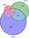 |
Fig. 1. Venn diagram showing the overlap between the three comparison samples S12 (Sbarrato et al. 2012), P17 (Paliya et al. 2017) and P21 (Paliya et al. 2021). |
4. The multiwavelength dataset
In this section, we describe the collection of multiwavelength data in the different bands, available for the 52 candidate PeVatron blazars. Optical spectroscopy constitutes the basis of our data sample. At these energies, we can delve into the mass accretion process on the central SMBH. Broad emission lines may appear in the spectra as a result of the gas of the BLR photoionized by the radiation produced in the accretion disk. The optical dataset is complemented with ancillary properties at radio and γ-ray energies.
4.1. Optical spectroscopy
We collected the data from public archives and the literature when available. We observed 12 objects for which neither a public spectrum was available in the archives, nor information in the literature (see also Table A.1 and Appendix E). For two of them, we acquired spectra with the European Southern Observatory (ESO) Very Large Telescope at Paranal Observatory (VLT) X-Shooter spectrograph (Vernet et al. 2011). The observations employed all three arms (NIR, VIS, and UVB) of the instrument. We observed three other targets using the R150 grism of the Gemini Multi-Object Spectrographs of Gemini South (GMOS-S, Murowinski et al. 1998; Gimeno et al. 2016). We observed seven additional targets with the R1000B grism of the Optical System for Imaging and low-Intermediate-Resolution Integrated Spectroscopy of the Gran Telescopio Canarias (GTC OSIRIS, Cepa et al. 2003). Further details on the complete spectroscopic dataset are provided in Appendix B.
4.2. Gamma-ray properties
When measured, the γ-ray luminosity of blazars is a good tracer of both the luminosity of the accretion disk and the power of the relativistic jet (Ghisellini et al. 2010; Sbarrato et al. 2014). The Lγ provides a lower limit on the power of the jet as some of the energy will inevitably go toward accelerating the plasma and, thus, it is proportional to the fraction of the energy that goes into radiation (Sbarrato et al. 2012). Among the candidate PeVatron blazars, 24 are detected in γ-rays. We collected the information for these sources from the Third Data Release of the Fourth Fermi Large Area Telescope (LAT) AGN Catalog (4LAC-DR3, Ajello et al. 2022), which encompasses frequencies between ν1 = 1.21 × 10²² Hz(50 MeV) and ν2 = 2.41 × 1027 Hz(1 TeV). To estimate the luminosity Lγ, we adopted the following method,
 (1)
(1)
Here dL is the luminosity distance of the source1, αγ = Γγ − 1 was evaluated from the photon spectral index Γγ in the LAT energy band (Ghisellini et al. 2009). Sγ(ν1,ν2) is the γ-ray energy flux between the frequencies ν1 and ν2, calculated as integration of a power-law spectrum over the Fermi-LAT band as,
![Mathematical equation: $$ \begin{aligned} S_{\gamma } \left( \nu _{1}, \nu _{2} \right) = {\left\{ \begin{array}{ll} \frac{\alpha _{\gamma } h \nu _{1} F_{\gamma }}{1 - \alpha _{\gamma }} \cdot \left[ \left( \frac{\nu _{2}}{\nu _{1}} \right)^{1 - \alpha _{\gamma }} -1 \right]&\text{ for } \alpha _{\gamma } \ne 1 , \\ h \nu _{1} F_{\gamma } \ln \left( \frac{\nu _{2}}{\nu _{1}} \right)&\text{ for } \alpha _{\gamma } = 1 \, \end{array}\right.} \end{aligned} $$](/articles/aa/full_html/2025/08/aa51328-24/aa51328-24-eq5.gif) (2)
(2)
where ![Mathematical equation: $ F_{\gamma} \left[ \mathrm{ph} \cdot \mathrm{cm}^{-2} \cdot \mathrm{s}^{-1} \right] $](/articles/aa/full_html/2025/08/aa51328-24/aa51328-24-eq6.gif) is the photon flux. For the remaining 28 blazars with no LAT detection, we placed an upper limit on the γ-ray luminosity considering the sensitivity of the instrument for a power-law-spectrum point-source and 10 yr exposure2 (Fγ = 5 × 10⁻¹⁰ ph ⋅ cm−2 ⋅ s−1, Γγ = 2.0). While these limits provide straightforward initial information about the jet’s power, they should be interpreted with caution. This is especially true for objects whose high-energy emission may elude detection in the LAT band (e.g., those expected to peak at γ-ray energies ≲MeV range).
is the photon flux. For the remaining 28 blazars with no LAT detection, we placed an upper limit on the γ-ray luminosity considering the sensitivity of the instrument for a power-law-spectrum point-source and 10 yr exposure2 (Fγ = 5 × 10⁻¹⁰ ph ⋅ cm−2 ⋅ s−1, Γγ = 2.0). While these limits provide straightforward initial information about the jet’s power, they should be interpreted with caution. This is especially true for objects whose high-energy emission may elude detection in the LAT band (e.g., those expected to peak at γ-ray energies ≲MeV range).
4.3. Radio properties
The radio power offers a complementary proxy for the intrinsic jet power (Sbarrato et al. 2014; Heckman & Best 2014), especially useful for objects with no detection at γ rays. Besides, the radio power P1.4 GHz yields further insights regarding the HERG–LERG nature (see Sects. 2 and 2.2). We used the radio information provided by 5BZCat. For each blazar, the catalog lists the radio flux density at 1.4 GHz from NRAO VLA Sky Survey (NVSS, Condon et al. 1998) or Very Large Array (VLA) Faint Images of the Radio Sky at Twenty-cm (FIRST, White et al. 1997).
5. Optical spectroscopy data analysis
5.1. Data reduction procedure
The first step was the reduction of the optical spectra for the sources that we observed. For the X-Shooter spectra, we used the EsoReflex version 2.11.5 pipeline (Freudling et al. 2013) and, for GMOS-S, the Data Reduction for Astronomy from Gemini Observatory North and South (DRAGONS) software v3.1.0 (Labrie et al. 2019). For the OSIRIS spectra, we used the PypeIt v1.16.0 pipeline (Prochaska et al. 2020). The reduction was performed through the standard steps of bias and dark current subtraction, flat field correction, and cosmic ray removal. The arc lamp exposures were reduced separately and used for the wavelength calibration. Then, sky subtraction was applied to remove the background contribution from the science spectra. The spectra of the correspondent standard star were also reduced separately and used for the estimation of the sensitivity curve. Finally, flux calibration was applied to the science data. After that, for the X-Shooter dataset, the Molecfit version 4.2.3 (Smette et al. 2015; Kausch et al. 2015) software tool was used to correct the science spectra for atmospheric contamination features, in particular the contribution of telluric absorption lines.
The remaining blazars in the sample were investigated using various pipelines to extract and examine spectra from different archives. The data taken from the Six-degree Field Galaxy Survey (6dFGS, Jones et al. 2004, 2009), and the 2dF QSO Redshift Survey (2QZ, Smith et al. 1998; Croom et al. 2004) catalogs are not flux calibrated, and in this case, we used the conversion factor ct = 7.69 × 10⁻¹⁷ erg ⋅ s−1 ⋅ cm−2⋅ Å−1 from photon counts to flux density units (Koss et al. 2017). For low-resolution spectra of the Large Sky Area Multi-Object Fiber Spectroscopic Telescope (LAMOST, Zhao et al. 2012), the flux calibration is relative. This affects the accuracy level of the absolute flux, which is in units of  . More details are provided in Appendix B.
5.2. Estimation of physical quantities
We extracted and visually inspected the optical spectra of interest to identify possible emission line profiles. The hydrogen recombination lines of the Lyman or Balmer series Lyα, Hα and Hβ are among the strongest lines detected in the environment of an AGN. They are produced in the BLR along with the more highly ionized permitted Mg ii, C ivlines. Instead, [O ii] and [O iii] spectral lines are emitted in the NLR and produced by forbidden transitions. Permitted transitions (e.g., those occurring in the BLR) are electric dipole transitions with high probabilities (∼105 − 109 s−1) and originate in regions of higher-density plasma (on average, ne ≳ 109 cm−3 in observed BLRs, Osterbrock & Ferland 2006). The observed broad line profiles are the result of permitted transitions, while forbidden transitions give rise to narrow profiles. For broad lines, the density of the forming region is so high that all levels of the ions that would be otherwise responsible for forbidden transitions are collisionally de-excited (Osterbrock & Ferland 2006). In forbidden transitions, electrons have much lower probabilities (∼10−6 − 102 s−1) of being excited to (or de-excited from) these levels and require very low electron densities ≲106 cm−3 to populate the levels above the ground state via electron collisions (Longair 1994).
We applied a rebinning of the spectra when needed, identified the lines, and then cross-checked the redshift available from the literature with our estimate. We used the SpectRes PYTHON tool (Carnall 2017) for the rebinning. Then, we used the Image Reduction and Analysis Facility (IRAF, Tody et al. 1986; Tody 1993) software to fit the detected lines with either one or multiple Gaussian functions according to the morphological shape of the profile. The results from the fit3 were extracted, compared to independent fits performed with SciPy4 and used for further analysis. We used the flux, EW, and full width at half maximum (FWHM) to estimate the central engine properties of the blazars in our sample (similarly to Celotti et al. 1997; Ghisellini & Tavecchio 2008; Shen et al. 2011; Shen & Liu 2012; Paliya et al. 2017; Padovani et al. 2019; Paliya et al. 2021). The total luminosity of the spectral line was estimated as  . The corresponding errors with the fitted quantities are usually ∼5% for the line flux and 10% for the FWHM (Decarli et al. 2008, 2011).
Thirteen targets lack BLR lines. They display either a featureless optical spectrum or only NLR lines. Therefore, for these, we estimated upper limits on the luminosity of the nondetected emission lines: a power-law fit was applied to a region of 500 Å at the position of the expected line, depending on the redshift (following the approach of Sbarrato et al. 2012). Then, we simulated an emission line of Gaussian profile with fixed FWHM  (Decarli et al. 2011) and flux Fline. We assumed an uncertainty of 10% on the flux Fline, and let Fline vary up to a maximum value of 1% of the fitted continuum. To determine the upper limit, we performed a χ2 test and accepted as flux limit, the value Fline for which χ2 < χ2(99%).
Thereafter, we employed the luminosity (or the upper limit) of the emission lines to infer the total luminosity of the broad line region,
 (3)
(3)
with Lrel. frac. = 77, 22, 34, 63 for Hα, Hβ, Mg iiand C iv, respectively, being the contribution of each line to the total BLR luminosity as estimated based on the composite spectrum of Francis et al. (1991), assuming a relative flux of 100 for Lyα. The total broad line flux is  (Francis et al. 1991). When more than one emission line was present in the spectrum, we estimated the BLR luminosity by averaging the measured line profiles (Celotti et al. 1997; Sbarrato et al. 2012).
To estimate the BLR luminosity, which is then used to infer the accretion regime, we used only the BLR line fluxes or limits. Although for some objects NLR lines are detected, and works suggest to use them to derive estimates for the BLR luminosity (Padovani et al. 2019, 2022a), based on our tests, the procedure leads to not fully consistent values of the accretion regime in our sample (Azzollini et al., in prep.). The luminosity of the disk is estimated by assuming a thin Shakura-Sunyaev accretion disk (Shakura & Sunyaev 1973) with BLR covering factor of 0.1 to it, so that LBLR ≃ 10% Ldisk (Sbarrato et al. 2012; Ghisellini et al. 2014). It directly links the accretion disk luminosity with the observed broad emission lines and provides an estimation independent of the viewing angle (the lines are assumed to be isotropically emitted) and it avoids contamination from the nonthermal continuum. The expected average uncertainty on the resulting value is a factor of 2 (Sbarrato et al. 2012; Ghisellini et al. 2014).
Optical spectral emission lines inform about the bolometric thermal luminosity of the accretion flow in AGN. To this end, we used the broad Hβ, Mg iilines and the narrow [O ii], [O iii] lines, when available (Punsly & Zhang 2011; Padovani et al. 2019),
 (4)
(4)
where the coefficients are (a,b)= (12.32 ± 0.20, 0.78 ± 0.01), (16.76±0.26,0.68±0.01), (26.50±0.32,0.46±0.01), (33.96±0.33,0.29±0.01) for Hβ, Mg ii, [O ii] and [O iii], respectively.
The luminosity and FWHM of the lines, and the empirical scaling laws of Shen et al. (2011) and Shen & Liu (2012) were employed in the estimation of the virial mass of the central black hole. The approach assumes that the BLR is gravitationally bounded to the central BH potential, in such a way that we can estimate the mass of the central object by evaluating the orbital radius and Doppler velocity of the region through an inspection of the emitted lines. The evaluation was made through the following equation:
 (5)
(5)
Here the coefficients are (Shen et al. 2011; McLure et al. 2004; Vestergaard & Osmer 2009),
 (6)
(6)
The typical uncertainty on the value of MBH is a factor of 4 (Vestergaard & Peterson 2006). From the black hole mass, we derived the Eddington luminosity of the sources as  (Eddington 1926; Lang 1974). The resulting value only depends on the mass of the central accreting object. By definition, it sets an upper limit on the accretion luminosity of the central compact core. Therefore, the disk luminosity in Eddington units traces the normalized accretion rate (Shen et al. 2011; Ghisellini et al. 2014)
  , where η is the radiative efficiency of accretion. For geometrically thin accretion disks, it depends on the location of the innermost stable orbit of the disk and the spin of the central black hole.
At Ldisk ≲ 10−2 LEdd, the accretion structure becomes radiatively inefficient, with the standard accretion disk turning into a hot accretion flow (ADAF). The dependence of the disk luminosity on the accretion rate changes ( ). This leads to an analogous change in the dependence of LBLR on Ṁ (Ghisellini et al. 2014; Sbarrato et al. 2014). However, the response of the jet to these different inner physical properties of the black hole is not known and remains an open debate.
In this model, the radiation component takes into account the contributions of the emission disk, the broad line region, the dusty torus surrounding the disk, and the part of the radiation that is intercepted in the IR and re-emitted. This structure allows us to estimate the size of the broad line region and the dusty torus from the luminosity of the disk. Following the works of Ghisellini & Tavecchio (2008), Ghisellini et al. (2014, 2017), we derive the radius of the BLR and the torus as
 (7)
(7)
 (8)
(8)
The resulting quantities are listed in Table A.2.
6. Comparison with reference blazar samples
In this section, we discuss the adopted approach and present the outcomes of our study. We investigated the physical properties of the sample of candidate neutrino-emitter blazars and the reference samples presented in Sect. 3.2 in light of the more physically driven approach we adopted. To this end, we focused on the accretion regime traced by the LBLR/LEdd and Lγ/LEdd, and the jet power traced by the radio power P1.4 GHz alongside the Lγ. The results for the accretion regime properties are presented in Fig. 2. Our sample (in black, with TXS 0506+056, PKS 1424+240, and 5BZB J0630-2406 highlighted in cyan, lime, and magenta, respectively; see Sect. 6.3 for further details) is compared to the γ-loud and γ-quiet blazars studied in P17 and P21 and the sources in S12 (see Sect. 3.2). The arrows indicate the estimated upper limits on either the optical and/or γ-ray luminosity (see also Appendix C). The dotted lines represent the distinction for the accretion efficiency regime, respectively LBLR/LEdd ∼ 5 × 10⁻⁴ and Lγ/LEdd ∼ 0.1 (Ghisellini et al. 2011b; Sbarrato et al. 2012, 2014). On the sides, the histograms show the distribution of the two ratios for all the samples, excluding estimated limits. The black solid lines indicate the median value for the candidate PeVatron blazars. In Fig. 3, the luminosity of the broad line region as a function of the radio power allowed us to study the disk-jet connection even in the sources that are not-detected at γ-rays (see a similar approach in Sbarrato et al. 2014). We compared our sample to the other samples (S12, P17, P21), cross-matching them with NVSS (Condon et al. 1998) and FIRST (White et al. 1997) to infer the P1.4 GHz.
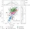 |
Fig. 2. LBLR/LEdd (accretion regime proxy) vs. Lγ/LEdd (power of the jet proxy) of the candidate PeVatron blazars (black). The three blue FSRQs (masquerading BL Lacs) TXS 0506+056, PKS 1424+240, and 5BZB J0630-2406 that were previously identified as promising neutrino-emitter blazar candidates are highlighted in cyan, lime, and magenta, respectively (see Sect. 6.3). As a comparison, the plot also shows the samples of S12, P17, and P21 (see Sect. 3.2). For P17, we plot the subsample with properties analyzed through optical spectroscopy. The arrows represent upper limits on either one or both of the shown quantities (see also Appendix C). The dotted gray lines represent the boundaries for the different accretion efficiencies, respectively LBLR/LEdd ∼ 5 × 10⁻⁴ and Lγ/LEdd ∼ 0.1 (Ghisellini et al. 2011b; Sbarrato et al. 2012). On the sides are the histograms of the corresponding quantities for all the samples, excluding all the upper limits. Here the black solid lines represent the median values for the candidate PeVatron blazars. |
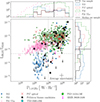 |
Fig. 3. Accretion regime LBLR/LEdd as a function of the radio power at 1.4 GHz, compared to the samples of (S12, P17, and P21 in the plot, Sbarrato et al. 2012; Paliya et al. 2017, 2021, see Sect. 3.2 for further details). For P17 we plot the subsample whose properties are analyzed through optical spectroscopy. The arrows indicate the upper limits on the optical luminosity. The three blue FSRQs (masquerading BL Lacs) TXS 0506+056, PKS 1424+240, and 5BZB J0630-2406 that were already identified as promising neutrino-emitter blazar candidates are highlighted in cyan, lime, and magenta, respectively (see Sect. 6.3). The dashed horizontal gray line represents the separation limits for the accretion efficiency LBLR/LEdd ∼ 5 × 10⁻⁴ (Ghisellini et al. 2011b; Sbarrato et al. 2012). Instead, the vertical dotted line is the threshold P1.4 GHz ∼ 1026 W ⋅ Hz−1 above which HERGs dominate over LERGs (Best & Heckman 2012; Padovani et al. 2019). On the sides are the normalized histograms of the corresponding quantities for the samples, excluding all the upper limits. Here, the black solid lines represent the median value for the candidate PeVatron blazars. |
Figure 4 shows the distribution of the other estimated quantities, i.e., the histograms of the redshift, black hole mass, disk luminosity, size of the BLR and DT, and γ-ray luminosity, aside from the accretion regime and the radio power, shown in Figs. 2–3. The vertical black solid line represents the median for our sample.
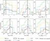 |
Fig. 4. Distribution of the redshift, black hole mass, disk luminosity, size of the broad line region and dusty torus, and γ-ray luminosity. The comparison samples are Sbarrato et al. (2012), Paliya et al. (2017, 2021) (S12, P17, P21, respectively), BZCat and 4LAC-DR3, with the exclusion of upper limits on the plotted quantity. The black solid lines correspond to the median value for the candidate PeVatron blazars. |
6.1. Statistical analysis procedure
We addressed to which extent the properties of the target sample, i.e., the candidate neutrino-emitter objects, are compatible with those of the other reference samples, by means of statistical tests. We quantified this first by using the Anderson-Darling (A-D) statistical test (Anderson & Darling 1952) on the physical properties of different populations, considering only the measurements of the interested quantity (i.e., excluding limits). As a check, we then included the upper limits, as if they were actual measurements, and by repeating the same analysis we verified that the overall findings of the A-D test remained consistent.
However, this approach is not ideal and has limited statistical power for samples which contain both measured values and a significant fraction of upper limits. To address this limitation, we explored the applicability of alternative methods that incorporate upper limits, as utilized in previous studies, i.e., the Kaplan-Meier estimator used in combination with the logrank and the Peto logrank statistical tests (e.g., Feigelson & Nelson 1985; Padovani 1992; Padovani et al. 2022b; Paiano et al. 2023).
To this end, the Kaplan-Meier estimator was used to estimate the survival function of a given physical property, in a stepwise manner, considering both measured values and including censored data (limits; similar to the approach in Lavalley et al. 1992; Feigelson & Nelson 1985; Isobe et al. 1986; Avni et al. 1980; Pfleiderer & Krommidas 1982). We, then, assessed the performance of the logrank and the Peto logrank tests for comparing survival curves across different samples through simulations, focusing in particular on Type I errors, i.e., false positives. As discussed in Appendix D, these methods are highly sensitive to the number and distribution of censored data points, as well as variations in sample sizes, requiring strong caution when interpreting the outcomes. Tailored investigations can assess the robustness of each statistically significant result individually (see Appendix D for further details). In this study, we present the results only for the Peto logrank test, which we found to be less affected by differences in the censoring patterns between the two samples (as previously discussed in Feigelson & Nelson 1985). For reference, we performed the analysis by using the PYTHON package lifelines5, and the ASURV routine (Lavalley et al. 1992), finding consistent results between the two.
The main findings are summarized in Table A.3. The first column reports the analyzed quantity, while the second, third, and fourth columns detail the tested samples, including the number of measurements and the number of upper limits either excluded or included in the analysis. The fifth and sixth columns present the resulting pre-trial pvalues from the A-D and Peto logrank tests, respectively. Our focus is on comparisons that yield significant results in the pre-trial Peto logrank test, noting that the corresponding A-D test outcomes generally follow those of the Peto logrank test. Before discussing the implications of the observed findings, there are a few caveats to note.
-
The tests we performed are strongly correlated. A statistically significant result in one test can increase the likelihood of significant findings in related tests, due to the inherent correlations among the variables. This interdependence can affect the interpretation of pvalues and the overall significance of the findings.
-
When conducting multiple statistical tests, the likelihood of observing at least one significant result due to chance increases, that is known as the look-elsewhere effect. To account for this, a correction is needed to limit the overall Type I error rate.
In this exploratory study, where identifying potential leads for further investigation is a priority, we used the Benjamini-Hochberg procedure to correct for trials (Benjamini & Hochberg 1995). This is suitable for independent and positively correlated tests, and offers a more balanced approach by controlling the false discovery rate (FDR), allowing for a higher rate of true discoveries while maintaining control over false positives.
To correct for trials, first we ranked the pre-trial pvalues in ascending order. For each pvalue, we computed the Benjamini-Hochberg critical value using the formula,
Critical Value = 
where i is the rank, m the total number of tests (i.e., 32 in our case), and Q the chosen FDR level (i.e., 0.003 in our case).
In this case, the Benjamini-Hochberg critical values are,
We identified that the third-ranked pre-trial pvalue, 1.53 × 10⁻⁴, obtained from comparing the radio power of the target sample to the S12 one, is the largest pvalue that does not exceed its corresponding critical value. Following the Benjamini-Hochberg procedure, all pvalues ranked up to and including this rank are considered statistically significant. They are highlighted with a * symbol in Table A.3 (see Appendix D).
6.2. Discussion
The three highest post-trial significances ( ≳ 3σ) are observed for the comparison of MBH between the target sample and P17, while the other two are found when comparing the redshift and P1.4 GHz with S12. All of the other quantities are found statistically compatible with the reference samples, according to the Benjamini−Hochberg test.
Comparing the MBH distributions between the target sample and the P17 sample, we observed a significance ( ≳ 3σ) and noted that the former sample includes 38% censored data. To assess the robustness of this result, we conducted simulations to evaluate potential biases introduced by the high rate of censored data. These simulations, presented in Appendix D, suggest that the observed discrepancy may arise from an intrinsic difference between the two samples. The mass distribution of the candidate PeVatron blazars extends to larger values, with two objects above ≳1010 M⊙ and with ∼35% of the objects (18 out of 52) above ≳109 M⊙, compared to the P17 sample, which instead comprises objects with MBH values up to 2.40 × 10⁹ M⊙, six of which (∼13%) above ≳109 M⊙. This suggests that our target sample tends to host more massive black holes than those in P17. However, no significant discrepancy is observed when compared to other reference samples, indicating that these properties remain consistent with the overall population of γ-loud blazars (P21) and sources with diverse accretion properties (S12).
Referring to Fig. 3, most candidate PeVatron blazars (∼63%) show powerful relativistic jets and occupy the region of the P1.4 GHz distribution dominated by HERGs (Padovani et al. 2022b; Kalfountzou et al. 2012; Best & Heckman 2012). In this case, the median value is  , above the P1.4 GHz ∼ 1026 W ⋅ Hz−1 HERG–LERG threshold. As displayed in Table A.3, the P1.4 GHz distribution of our sample is compatible with the other samples except in the case of S12, for which a difference at ≳3σ level with the Peto logrank is found. A similar difference is found with the redshift distribution of S12. The distributions of the S12 sample are skewed toward lower redshifts and reduced radio powers relative to our sample. Among the S12 sample, only the 29% of the objects (40 out of 138) lie above P1.4 GHz ≳ 1026 W ⋅ Hz−1. As mentioned in Sect. 3.2, the S12 reference sample allows for an exploration of the full parameter space of HERG and LERG populations. These findings reinforce, from both the P1.4 GHz and redshift distribution perspectives, the mild tendency shown by the candidate neutrino-emitting blazars to preferably exhibiting HERG-like characteristics.
A consistent picture to the P1.4 GHz distribution emerges looking at the LBLR/LEdd properties: candidate PeVatron blazars show a mild preference (∼61%) for populating the region of the LBLR/LEdd occupied by sources with efficient accretion properties and, therefore, by HERG-like objects. Although from a statistical standpoint their accretion properties remain consistent with those of the other samples, the effectiveness of these tests is limited by the presence of a large number of censored data. As shown in Fig. 2, our sample displays a median value  and
and  . When excluding objects with upper limits, as expected, ∼87% occupy the HERG region, with
  and
and  .
.
For what concerns the γ-ray luminosity, the blazars in our sample (24 γ-loud and 28 γ-quiet) are distributed among a broad range of values, from 1.43 × 1042 erg ⋅ s−1 to 1.21 × 1048 erg ⋅ s−1. The median value of the detections is  , and the 79% lies between 1044 ≲ Lγ ≲ 1047 erg ⋅ s−1. In terms of γ-ray luminosity, the candidate PeVatron blazars are compatible with the overall population, as suggested by the results of the Peto logrank test with the 5BZCat and 4LAC-DR3.
6.3. Blue FSRQs – masquerading BL Lacs among the candidate PeVatron blazars
Among the sample of candidate PeVatron blazars, four objects had been proposed as blue FSRQs (masquerading BL Lacs) in the literature: TXS 0506+056, PKS 1424+240, 5BZB J0630-2406, and 5BZB J0035+1515. In this work, we conclude that the first three of them share HERG-like characteristics. Based on our newly acquired optical data of the fourth object, we establish the LERG nature of 5BZB J0035+1515.
The candidate IceCube neutrino source TXS 0506+056 (5BZB J0509+0541), was identified as belonging to the subclass of masquerading BL Lacs following the detection of the [O ii] and [O iii] lines in an optical spectrum taken with the Gran Telescopio Canarias (GTC) between the end of 2017 and the beginning of 2018 (Paiano et al. 2018; Padovani et al. 2019). Historically classified as a BL Lac, the HERG nature of this source is supported by the high radio power and [O ii], [O iii] luminosity (P1.4 GHz ∼ 1.8 × 1026 W ⋅ Hz−1 and L[O II], [O III] ∼ 2 × 1041 erg · s−1, respectively) and the accretion regimes LBLR/LEdd ∼ 10−3, Lγ/LEdd ∼ 0.7 (Padovani et al. 2019).
Similarly, the PeVatron blazar candidate PKS 1424+240 (5BZB J1427+2348) has been previously identified as a potential neutrino source and blue FSRQ (masquerading BL Lac). PKS 1424+240 displayed [O ii] and [O iii] emission lines in a Gran Telescopio Canarias (GTC) spectrum taken in 2015 (Paiano et al. 2017). It was proposed as a HERG object based on the high power P1.4 GHz ∼ 5 × 1026 W ⋅ Hz−1, L[O II] ∼ 4×1041 erg·s−1, and efficient accretion regimes LBLR/LEdd ≳ 1.5 × 10⁻³, Lγ/LEdd > 2 (Padovani et al. 2022a).
5BZB J0630-2406 has been traditionally classified as a BL Lac object. Ghisellini et al. (2012) highlighted its high power, unusual for BL Lacs, and proposed that it belongs to the subclass of blue FSRQ (masquerading BL Lacs). We analyzed the VLT spectrum obtained by Shaw et al. (2013) in 2012. We confirmed the absence of emission lines in the spectrum, and the lower limit estimate z ≳ 1.239 for the redshift, which was placed by the authors based on the absorption features. A recent study estimated an upper limit z < 1.33 based on the effect of the extragalactic background light attenuation (Lainez et al. 2024).
Assuming the value of z ≳ 1.239, we placed an upper limit on the luminosities of the Mg ii λ2798 Å and [O II]λ3727 Å lines as explained in Sect. 5.2. We found Ldisk < 2.53 × 1045 erg ⋅ s−1, LBLR/LEdd < 5.79 × 10⁻⁴ and Lγ/LEdd ∼ 1.02. In the plot of Figure 2 it is located next to TXS 0506+056 and PKS 1424+240, within the HERG regime. The inferred black hole mass is < 3.79 × 10⁹, which is toward the upper hand of the values usually observed. We note that a lower BH mass estimate than this limit would lead to a higher accretion efficiency, keeping the validity of the HERG-nature hypothesis.
The nature of this blazar appears consistent with the HERG-like behavior, as further supported by its radio power P1.4 GHz = 9.64 × 1026 W ⋅ Hz−1 and theoretical modeling. In a previous study, we modeled the quasi-simultaneous broadband spectral energy distribution of 5BZB J0630-2406, revealing that the source hosts a luminous (Ldisk ∼ 4 × 1045 erg ⋅ s−1) accretion disk with accretion rates LBLR/LEdd ∼ 2 × 10⁻⁴, Lγ/LEdd ∼ 0.15 and dissipation radius on the outer edge of the BLR (Fichet de Clairfontaine et al. 2023). The conclusions are in agreement with the results of Ghisellini et al. (2012), in which a limit Ldisk ∼ 5.5 × 1045 erg ⋅ s−1 was obtained using an empirical relation between LBLR − Lγ6, and are in agreement with this work. The overall findings suggest the likely presence of external radiation fields (accretion disk, narrow and broad line regions) whose emission is overcome by the jet’s synchrotron emission.
The nature of 5BZB J0035+1515 as blue FSRQ was discussed in previous works (Ghisellini et al. 2012; Padovani et al. 2012). Starting from the featureless SDSS spectrum available for this source, the works assumed an average mass MBH = 5 × 10⁸ M⊙ and adopted the photometric redshift z = 1.28 to derive the values Lγ ∼ 1045erg ⋅ s−1, LBLR < 3 × 1044erg ⋅ s−1 and P1.4 GHz = 1.58 × 1026 W ⋅ Hz−1, leading to the blue FSRQ scenario. However, the lack of a spectroscopic redshift determination at the time prevented the authors to settle the debate. As noted, a smaller value of the redshift would result in lower luminosity estimations and different conclusions, i.e., the source is intrinsically a LERG (Ghisellini et al. 2012). Our new GTC OSIRIS observation resulted in the detection of Mg ii and [O ii] emission lines. We estimated a redshift of z = 0.57, which is consistent with the lower limit of z > 0.55 reported (Paiano et al. 2017). We derived LBLR/LEdd ∼ 1.79 × 10⁻⁴ and Lγ/LEdd ∼ 0.182, while for the radio power, we found a value below the ∼1026 W ⋅ Hz−1. Therefore, we conclude that 5BZB J0035+1515 belongs to the LERG class, based on the accretion regime and radio power properties. This is consistent with what was already foreseen in case of a redshift lower than the photometric estimation (Ghisellini et al. 2012).
Adopting the physically motivated classification describes the three known blue FSRQs (masquerading BL Lacs) TXS 0506+056, PKS 1424+240, and 5BZB J0630-2406 included in our sample with less ambiguity as high emitting power sources with their broad emission lines swamped by the jet synchrotron emission (Giommi et al. 2013; Padovani et al. 2022b). The implications of their intrinsic nature are explored in further detail in the next Sect. 6.4 in the context of neutrino stacking studies. TXS 0506+056, PKS 1424+240, and 5BZB J0630-2406 are highlighted in cyan, lime, and magenta in Figs. 2–3. Their location beside the other HERG-like sources is consistent with the mild tendency shown by the candidate PeVatron blazars to preferentially exhibit intense radiation fields, radiatively efficient accretion and powerful jets.
6.4. Implications for neutrino multimessenger studies
Several studies have been hampered by blindly adhering to the historical categorization of objects, sometimes relying solely on catalog classifications or attempting to fit them in observation-based schemes, leading to classifications that change over time (Antonucci 2012). A notorious example in the field of multimessenger neutrino astrophysics is TXS 0506+056, the first probable high-energy neutrino source. Due to its featureless optical spectrum, historically it was classified as a BLL and therefore considered a LERG-like object with no prominent radiation fields. Later, it was proposed to be an FSRQ-like object, therefore being intrinsically a HERG. As addressed in the previous section, this is not a standalone case in the context of candidate neutrino-emitter blazars. The impact on previous neutrino studies focused on blazars may be not negligible.
For instance, several works investigated the contribution of γ-ray blazars to the IceCube neutrino diffuse flux (Aartsen et al. 2017a). The studies performed a neutrino stacking analysis of the whole blazar sample, along with an analysis of the separate BLL and FSRQ subsamples. They derived limits on the maximal contributions to the diffuse neutrino flux: 19%−27% for the whole blazar sample; 3%−13% for BL Lacs, and 5%−17% for FSRQs (Aartsen et al. 2017a).
The rationale behind examining different blazar subpopulations was due to their distinct physical environments and potential neutrino production mechanisms. In FSRQs, characterized by strong radiation fields, the leading hypothesis for neutrino production is proton-photon interactions. In contrast, BL Lacs, with no or weaker radiation fields, are hypothesized to produce neutrinos primarily through proton-synchrotron mechanisms (Mücke et al. 2003). In light of their observational-driven classification, the aforementioned stacking study listed TXS 0506+056, PKS 1424+240, and 5BZB J0630-2406 among the BLL subsample. However, as discussed in Sect. 6.3, they belong to the HERG class and display quasar-like properties, hence should be accounted for within the FSRQ subsample. As pointed out by our earlier works (PAPER I, PAPER II), these promising neutrino-emitters are associated with fairly prominent anisotropies in the time-integrated IceCube skymap, therefore their contribution to a stacking analysis would unlikely be negligible. Similar objects may be present in the considered sample of γ-ray blazars, and erroneously included in the BL Lacs subpopulation. Our findings advocate for the need to embrace the physical-driven selection of blazars and put into question the limits (possibly also the nondetection) derived from the individual subsamples.
7. Summary and conclusions
In this work we studied a selected sample of candidate neutrino-emitter blazars proposed as counterparts of IceCube hotspots (i.e., the 52 candidate PeVatron blazars), using a multiwavelength approach, collecting information in optical, radio, and γ-rays. The sample includes sources classified both as BL Lacs and FSRQs according to the traditional scheme based on the EW of the spectral lines. To infer the nature of these objects, we adopted a physically driven approach, which allowed us to pinpoint with less ambiguity the HERGs or LERGs properties (Ghisellini et al. 2011b; Sbarrato et al. 2012, 2014; Best & Heckman 2012; Padovani et al. 2022b). To this end, we investigated the mass accretion properties of the central engine and the relativistic jet power. We performed statistical tests to compare the properties of our target sample of candidate neutrino-emitter blazars with reference samples from the literature. We explored the applicability of methods that include limits in the analysis, showing that these are highly sensitive to the number and distributions of limits, and sample sizes, requiring caution when interpreting the results.
Our work suggests discrepancies at the ≳3σ level post-trial in three cases, where the black hole mass, redshift and radio power of the candidate PeVatron blazars extend to larger values compared to two of the reference samples. The findings suggest that these blazars are more HERG-like in terms of jet power, as evidenced by a slightly higher representation of HERG sources. This may indicate a preference for objects with higher accretion efficiency, stronger radiation fields, and significant radio power. In a multimessenger view, this would be consistent with theoretical models that predict enhanced neutrino production in such environments (Dermer et al. 2014), and with evidence supporting radio-bright objects as neutrino candidate emitters (Plavin et al. 2020, 2021; Zhou et al. 2021; Kun et al. 2022; Plavin et al. 2023; Kovalev et al. 2023; Kouch et al. 2024).
The presence of blue FSRQs (also known as masquerading BLLs) among candidate PeVatron blazars warrants caution in interpreting previous stacking studies that constrain the diffuse flux contribution from different blazar subpopulations. Our findings challenge the limit, and potentially even the nondetection, derived from individual subsamples (Aartsen et al. 2017a), and emphasize the need for a physically driven selection of blazars. While our statistical analysis did not provide conclusive evidence for a difference in the overall behavior of the candidate neutrino-emitter blazars, this initial investigation of the candidate PeVatron blazar sample revealed a broad range of properties. The challenge in confirming individual neutrino – blazar associations currently limits definitive conclusions about the properties of candidate neutrino-emitter blazars. Future dedicated studies will focus on assessing the genuineness of these associations to shed light on the connection between blazars and neutrinos.
The estimation employs the value of the redshift and the Astropy cosmology package. For more details, see https://docs.astropy.org/en/stable/cosmology/index.html
See https://www.slac.stanford.edu/exp/glast/groups/canda/lat_Performance.htm for further details.
Splot function for profile deblending and Gaussian fitting: https://astro.uni-bonn.de/~sysstw/lfa_html/iraf/noao.onedspec.splot.html
See https://lifelines.readthedocs.io/en/latest/Survival%20analysis%20with%20lifelines.html for further details.
The empirical relation links the BLR and γ-ray luminosity through  (see Sbarrato et al. (2012), Ghisellini et al. (2012) for further details).
Acknowledgments
The authors thank the anonymous referee for the insightful comments that helped improve the manuscript. We are thankful to Andrea Tramacere, Stefano Marchesi, Marco Ajello, Paola Marziani, Nicola Masetti, Roger Romani, and Karl Mannheim for the constructive discussions. AA thanks German Gimeno and Kathleen Labrie for their support during the phases of observation and reduction of the Gemini data, and Tapio Pursimo for the help with the NOT spectrum. This work was supported by the European Research Council, ERC Starting grant MessMapp, S.B. Principal Investigator, under contract no. 949555. Based on observations collected at the European Southern Observatory under ESO programs 109.22WZ.001, 109.22WZ.001, 084.B − 0711(A), 087.B − 0614(A), 077.B − 0045. Based on observations obtained at the international Gemini Observatory, a program of NSF’s NOIRLab [Program ID GS-2022B-DD-201], which is managed by the Association of Universities for Research in Astronomy (AURA) under a cooperative agreement with the National Science Foundation on behalf of the Gemini Observatory partnership: the National Science Foundation (United States), National Research Council (Canada), Agencia Nacional de Investigación y Desarrollo (Chile), Ministerio de Ciencia, Tecnología e Innovación (Argentina), Ministério da Ciência, Tecnologia, Inovações e Comunicações (Brazil), and Korea Astronomy and Space Science Institute (Republic of Korea). This work is (partly) based on data obtained with the instrument OSIRIS, built by a Consortium led by the Instituto de Astrofísica de Canarias in collaboration with the Instituto de Astronomía of the Universidad Autónoma de México. OSIRIS was funded by GRANTECAN and the National Plan of Astronomy and Astrophysics of the Spanish Government. This work is (partly) based on data from the GTC Public Archive at CAB (INTA-CSIC), developed in the framework of the Spanish Virtual Observatory project supported by the Spanish MINECO through grants AYA 2011-24052 and AYA 2014-55216. The system is maintained by the Data Archive Unit of the CAB (INTA-CSIC). This research has made use of the NASA/IPAC Extragalactic Database, which is funded by the National Aeronautics and Space Administration and operated by the California Institute of Technology. Guoshoujing Telescope (the Large Sky Area Multi-Object Fiber Spectroscopic Telescope LAMOST) is a National Major Scientific Project built by the Chinese Academy of Sciences. Funding for the project has been provided by the National Development and Reform Commission. LAMOST is operated and managed by the National Astronomical Observatories, Chinese Academy of Sciences. The 2dF QSO Redshift Survey (2QZ) was compiled by the 2QZ survey team from observations made with the 2-degree Field on the Anglo-Australian Telescope. Funding for the Sloan Digital Sky Survey IV has been provided by the Alfred P. Sloan Foundation, the U.S. Department of Energy Office of Science, and the Participating Institutions. SDSS-IV acknowledges support and resources from the Center for High-Performance Computing at the University of Utah. The SDSS website is http://www.sdss4.org. SDSS-IV is managed by the Astrophysical Research Consortium for the Participating Institutions of the SDSS Collaboration including the Brazilian Participation Group, the Carnegie Institution for Science, Carnegie Mellon University, Center for Astrophysics | Harvard & Smithsonian, the Chilean Participation Group, the French Participation Group, Instituto de Astrofísica de Canarias, The Johns Hopkins University, Kavli Institute for the Physics and Mathematics of the Universe (IPMU)/University of Tokyo, the Korean Participation Group, Lawrence Berkeley National Laboratory, Leibniz Institut für Astrophysik Potsdam (AIP), Max-Planck-Institut für Astronomie (MPIA Heidelberg), Max-Planck-Institut für Astrophysik (MPA Garching), Max-Planck-Institut für Extraterrestrische Physik (MPE), National Astronomical Observatories of China, New Mexico State University, New York University, University of Notre Dame, Observatário Nacional/MCTI, The Ohio State University, Pennsylvania State University, Shanghai Astronomical Observatory, United Kingdom Participation Group, Universidad Nacional Autónoma de México, University of Arizona, University of Colorado Boulder, University of Oxford, University of Portsmouth, University of Utah, University of Virginia, University of Washington, University of Wisconsin, Vanderbilt University, and Yale University. This research has made use of the SIMBAD database, operated at CDS, Strasbourg, France. Part of this work is based on archival data, software, or online services provided by the Space Science Data Center – ASI.
References
- Aartsen, M. G., Abraham, K., Ackermann, M., et al. 2016, ApJ, 833, 3 [Google Scholar]
- Aartsen, M. G., Abraham, K., Ackermann, M., et al. 2017a, ApJ, 835, 45 [Google Scholar]
- Aartsen, M. G., Abraham, K., Ackermann, M., et al. 2017b, ApJ, 835, 151 [Google Scholar]
- Aartsen, M. G., Ackermann, M., Adams, J., et al. 2020, Phys. Rev. Lett., 124, 051103 [Google Scholar]
- Abbasi, R., Ackermann, M., Adams, J., et al. 2022, Science, 378, 538 [CrossRef] [PubMed] [Google Scholar]
- Abdo, A. A., Ackermann, M., Ajello, M., et al. 2009, ApJS, 183, 46 [NASA ADS] [CrossRef] [Google Scholar]
- Abdo, A. A., Ackermann, M., Ajello, M., et al. 2010, ApJ, 715, 429 [Google Scholar]
- Abdurro’uf, Accetta, K., Aerts, C., et al. 2022, ApJS, 259, 35 [NASA ADS] [CrossRef] [Google Scholar]
- Acero, F., Ackermann, M., Ajello, M., et al. 2015, ApJS, 218, 23 [Google Scholar]
- Adelman-McCarthy, J. K., Agüeros, M. A., Allam, S. S., et al. 2008, ApJS, 175, 297 [NASA ADS] [CrossRef] [Google Scholar]
- Ahumada, R., Allende Prieto, C., Almeida, A., et al. 2020, ApJS, 249, 3 [NASA ADS] [CrossRef] [Google Scholar]
- Ajello, M., Baldini, L., Ballet, J., et al. 2022, ApJS, 263, 24 [NASA ADS] [CrossRef] [Google Scholar]
- Anderson, T., & Darling, D. 1952, Ann. Math. Stat., 23, 193 [Google Scholar]
- Antonucci, R. 2012, Astron. Astrophys. Transac., 27, 557 [Google Scholar]
- Appenzeller, I., Fricke, K., Fürtig, W., et al. 1998, The Messenger, 94, 1 [NASA ADS] [Google Scholar]
- Avni, Y., Soltan, A., Tananbaum, H., & Zamorani, G. 1980, ApJ, 238, 800 [Google Scholar]
- Baldi, R. D., Laor, A., Behar, E., et al. 2022, MNRAS, 510, 1043 [Google Scholar]
- Ballet, J., Burnett, T. H., Digel, S. W., & Lott, B. 2020, arXiv e-prints [arXiv:2005.11208] [Google Scholar]
- Barbano, E., Buson, S., de Clairfontaine, G. F., et al. 2023, PoS, ICRC2023, 1540 [Google Scholar]
- Bellenghi, C., Padovani, P., Resconi, E., & Giommi, P. 2023, arXiv e-prints [arXiv:2309.03115] [Google Scholar]
- Benjamini, Y., & Hochberg, Y. 1995, J. Roy. Stat. Soc.: Ser. B (Methodol.), 57, 289 [Google Scholar]
- Best, P. N., & Heckman, T. M. 2012, MNRAS, 421, 1569 [NASA ADS] [CrossRef] [Google Scholar]
- Blandford, R. D., & Payne, D. G. 1982, MNRAS, 199, 883 [CrossRef] [Google Scholar]
- Blandford, R. D., & Znajek, R. L. 1977, MNRAS, 179, 433 [NASA ADS] [CrossRef] [Google Scholar]
- Bondi, H. 1952, MNRAS, 112, 195 [Google Scholar]
- Böttcher, M., Reimer, A., Sweeney, K., & Prakash, A. 2013, ApJ, 768, 54 [Google Scholar]
- Buson, S., Tramacere, A., Pfeiffer, L., et al. 2022a, ApJ, 933, L43 [NASA ADS] [CrossRef] [Google Scholar]
- Buson, S., Tramacere, A., Pfeiffer, L., et al. 2022b, ApJ, 934, L38 [Google Scholar]
- Buson, S., Tramacere, A., Oswald, L., et al. 2023, arXiv e-prints [arXiv:2305.11263] [Google Scholar]
- Cao, X., & Jiang, D. R. 1999, MNRAS, 307, 802 [NASA ADS] [CrossRef] [Google Scholar]
- Carnall, A. C. 2017, arXiv e-prints [arXiv:1705.05165] [Google Scholar]
- Celotti, A., Padovani, P., & Ghisellini, G. 1997, MNRAS, 286, 415 [NASA ADS] [CrossRef] [Google Scholar]
- Cepa, J., Aguiar-Gonzalez, M., Bland-Hawthorn, J., et al. 2003, in Instrument Design and Performance for Optical/Infrared Ground-based Telescopes, eds. M. Iye, & A. F. M. Moorwood, SPIE Conf. Ser., 4841, 1739 [NASA ADS] [CrossRef] [Google Scholar]
- Cerruti, M. 2020, Galaxies, 8, 72 [NASA ADS] [CrossRef] [Google Scholar]
- Chen, Y., Gu, Q., Fan, J., et al. 2021, ApJ, 913, 93 [NASA ADS] [CrossRef] [Google Scholar]
- Condon, J. J., Cotton, W. D., Greisen, E. W., et al. 1998, AJ, 115, 1693 [Google Scholar]
- Croom, S. M., Smith, R. J., Boyle, B. J., et al. 2004, MNRAS, 349, 1397 [NASA ADS] [CrossRef] [Google Scholar]
- Decarli, R., Labita, M., Treves, A., & Falomo, R. 2008, MNRAS, 387, 1237 [NASA ADS] [CrossRef] [Google Scholar]
- Decarli, R., Dotti, M., & Treves, A. 2011, MNRAS, 413, 39 [CrossRef] [Google Scholar]
- Deconto-Machado, A., del Olmo Orozco, A., Marziani, P., Perea, J., & Stirpe, G. M. 2023, A&A, 669, A83 [NASA ADS] [CrossRef] [EDP Sciences] [Google Scholar]
- Dermer, C. D., Murase, K., & Inoue, Y. 2014, J. High Energy Astrophys., 3, 29 [NASA ADS] [Google Scholar]
- Drinkwater, M. J., Webster, R. L., Francis, P. J., et al. 1997, MNRAS, 284, 85 [NASA ADS] [Google Scholar]
- Du, L. M., Bai, J. M., & Xie, Z. H. 2013, New A, 18, 1 [Google Scholar]
- Dwelly, T., Salvato, M., Merloni, A., et al. 2017, MNRAS, 469, 1065 [Google Scholar]
- Eddington, A. S. 1926, The Internal Constitution of the Stars (Cambridge University Press) [Google Scholar]
- Fan, J. H., Yang, J. H., Liu, Y., et al. 2016, ApJS, 226, 20 [CrossRef] [Google Scholar]
- Feigelson, E. D., & Nelson, P. I. 1985, ApJ, 293, 192 [NASA ADS] [CrossRef] [Google Scholar]
- Fichet de Clairfontaine, G., Buson, S., Pfeiffer, L., et al. 2023, ApJ, 958, L2 [NASA ADS] [CrossRef] [Google Scholar]
- Fischer, J. U., Hasinger, G., Schwope, A. D., et al. 1998, Astron. Nachr., 319, 347 [NASA ADS] [CrossRef] [Google Scholar]
- Fossati, G., Maraschi, L., Celotti, A., Comastri, A., & Ghisellini, G. 1998, MNRAS, 299, 433 [Google Scholar]
- Francis, P. J., Hewett, P. C., Foltz, C. B., et al. 1991, ApJ, 373, 465 [NASA ADS] [CrossRef] [Google Scholar]
- Freudling, W., Romaniello, M., Bramich, D. M., et al. 2013, A&A, 559, A96 [NASA ADS] [CrossRef] [EDP Sciences] [Google Scholar]
- Ghisellini, G., & Celotti, A. 2001, A&A, 379, L1 [NASA ADS] [CrossRef] [EDP Sciences] [Google Scholar]
- Ghisellini, G., & Tavecchio, F. 2008, MNRAS, 387, 1669 [NASA ADS] [CrossRef] [Google Scholar]
- Ghisellini, G., Maraschi, L., & Tavecchio, F. 2009, MNRAS, 396, L105 [NASA ADS] [Google Scholar]
- Ghisellini, G., Tavecchio, F., Foschini, L., et al. 2010, MNRAS, 402, 497 [Google Scholar]
- Ghisellini, G., Tagliaferri, G., Foschini, L., et al. 2011a, MNRAS, 411, 901 [Google Scholar]
- Ghisellini, G., Tavecchio, F., Foschini, L., & Ghirlanda, G. 2011b, MNRAS, 414, 2674 [NASA ADS] [CrossRef] [Google Scholar]
- Ghisellini, G., Tavecchio, F., Foschini, L., et al. 2012, MNRAS, 425, 1371 [NASA ADS] [CrossRef] [Google Scholar]
- Ghisellini, G., Tavecchio, F., Maraschi, L., Celotti, A., & Sbarrato, T. 2014, Nature, 515, 376 [NASA ADS] [CrossRef] [Google Scholar]
- Ghisellini, G., Righi, C., Costamante, L., & Tavecchio, F. 2017, MNRAS, 469, 255 [NASA ADS] [CrossRef] [Google Scholar]
- Gimeno, G., Roth, K., Chiboucas, K., et al. 2016, in Ground-based and Airborne Instrumentation for Astronomy VI, eds. C. J. Evans, L. Simard,&H. Takami, SPIE Conf. Ser., 9908, 99082S [NASA ADS] [Google Scholar]
- Giommi, P., Padovani, P., Polenta, G., et al. 2012, MNRAS, 420, 2899 [NASA ADS] [CrossRef] [Google Scholar]
- Giommi, P., Padovani, P., & Polenta, G. 2013, MNRAS, 431, 1914 [CrossRef] [Google Scholar]
- Graham, A. W. 2007, MNRAS, 379, 711 [NASA ADS] [CrossRef] [Google Scholar]
- Healey, S. E., Romani, R. W., Taylor, G. B., et al. 2007, ApJS, 171, 61 [Google Scholar]
- Healey, S. E., Romani, R. W., Cotter, G., et al. 2008, ApJS, 175, 97 [Google Scholar]
- Heckman, T. M., & Best, P. N. 2014, ARA&A, 52, 589 [Google Scholar]
- Hewett, P. C., & Wild, V. 2010, MNRAS, 405, 2302 [NASA ADS] [Google Scholar]
- Homan, D. C., Cohen, M. H., Hovatta, T., et al. 2021, ApJ, 923, 67 [NASA ADS] [CrossRef] [Google Scholar]
- Hovatta, T., Lindfors, E., Kiehlmann, S., et al. 2021, A&A, 650, A83 [NASA ADS] [CrossRef] [EDP Sciences] [Google Scholar]
- IceCube Collaboration 2013, Science, 342, 1242856 [Google Scholar]
- IceCube Collaboration (Aartsen, M. G., et al.) 2018, Science, 361, eaat1378 [NASA ADS] [Google Scholar]
- Inskip, K. J., Tadhunter, C. N., Morganti, R., et al. 2010, MNRAS, 407, 1739 [Google Scholar]
- Isobe, T., Feigelson, E. D., & Nelson, P. I. 1986, ApJ, 306, 490 [Google Scholar]
- Jones, D. H., Saunders, W., Colless, M., et al. 2004, MNRAS, 355, 747 [NASA ADS] [CrossRef] [Google Scholar]
- Jones, D. H., Read, M. A., Saunders, W., et al. 2009, MNRAS, 399, 683 [Google Scholar]
- Kalfountzou, E., Jarvis, M. J., Bonfield, D. G., & Hardcastle, M. J. 2012, MNRAS, 427, 2401 [NASA ADS] [CrossRef] [Google Scholar]
- Kausch, W., Noll, S., Smette, A., et al. 2015, A&A, 576, A78 [NASA ADS] [CrossRef] [EDP Sciences] [Google Scholar]
- Koss, M., Trakhtenbrot, B., Ricci, C., et al. 2017, ApJ, 850, 74 [Google Scholar]
- Kouch, P. M., Lindfors, E., Hovatta, T., et al. 2024, A&A, 690, A111 [NASA ADS] [CrossRef] [EDP Sciences] [Google Scholar]
- Kovalev, Y. Y., Plavin, A. V., Pushkarev, A. B., & Troitsky, S. V. 2023, Galaxies, 11, 84 [NASA ADS] [CrossRef] [Google Scholar]
- Krauß, F., Deoskar, K., Baxter, C., et al. 2018, A&A, 620, A174 [EDP Sciences] [Google Scholar]
- Kun, E., Bartos, I., Becker Tjus, J., et al. 2022, ApJ, 934, 180 [NASA ADS] [CrossRef] [Google Scholar]
- Labrie, K., Anderson, K., Cárdenes, R., Simpson, C., & Turner, J. E. H. 2019, in Astronomical Data Analysis Software and Systems XXVII, eds. P. J. Teuben, M. W. Pound, B. A. Thomas, & E. M. Warner, ASP Conf. Ser., 523, 321 [Google Scholar]
- Lainez, M., Dominguez, A., Paliya, V. S., et al. 2024, 38th International Cosmic Ray Conference, 558 [Google Scholar]
- Landoni, M., Falomo, R., Paiano, S., & Treves, A. 2020, ApJS, 250, 37 [NASA ADS] [CrossRef] [Google Scholar]
- Lang, K. 1974, Astrophysical Formulae: Volume I & Volume II: Radiation, Gas Processes and High Energy Astrophysics/Space, Time, Matter and Cosmology (Springer Science& Business Media) [Google Scholar]
- Lavalley, M., Isobe, T., & Feigelson, E. 1992, in Astronomical Data Analysis Software and Systems I, eds. D. M. Worrall, C. Biemesderfer, & J. Barnes, ASP Conf. Ser., 25, 245 [Google Scholar]
- León-Tavares, J., Valtaoja, E., Chavushyan, V. H., et al. 2011, MNRAS, 411, 1127 [Google Scholar]
- Longair, M. S. 1994, High Energy Astrophysics. Vol. 2: Stars, the Galaxy and the Interstellar Medium (Cambridge University Press), 2 [Google Scholar]
- Mannheim, K. 1993, A&A, 269, 67 [NASA ADS] [Google Scholar]
- Maraschi, L., & Tavecchio, F. 2003, ApJ, 593, 667 [Google Scholar]
- Massaro, F., D’Abrusco, R., Ajello, M., Grindlay, J. E., & Smith, H. A. 2011, ApJ, 740, L48 [NASA ADS] [CrossRef] [Google Scholar]
- Massaro, E., Maselli, A., Leto, C., et al. 2014, Multifrequency Catalogue of Blazars, 5th edn. [Google Scholar]
- Massaro, F., Landoni, M., D’Abrusco, R., et al. 2015, A&A, 575, A124 [NASA ADS] [CrossRef] [EDP Sciences] [Google Scholar]
- McLure, R. J., & Dunlop, J. S. 2004, in Multiwavelength AGN Surveys, eds. R.~ Mújica, & R. Maiolino, 389 [Google Scholar]
- Mingo, B., Hardcastle, M. J., Croston, J. H., et al. 2014, MNRAS, 440, 269 [Google Scholar]
- Morris, S. L., Stocke, J. T., Gioia, I. M., et al. 1991, ApJ, 380, 49 [Google Scholar]
- Mücke, A., Protheroe, R. J., Engel, R., Rachen, J. P., & Stanev, T. 2003, Astropart. Phys., 18, 593 [Google Scholar]
- Murowinski, R. G., Bond, T., Crampton, D., et al. 1998, in Optical Astronomical Instrumentation, ed. S. D’Odorico, SPIE Conf. Ser., 3355, 188 [Google Scholar]
- Nolan, P. L., Abdo, A. A., Ackermann, M., et al. 2012, ApJS, 199, 31 [Google Scholar]
- Osmer, P. S., Porter, A. C., & Green, R. F. 1994, ApJ, 436, 678 [Google Scholar]
- Osterbrock, D. E., & Ferland, G. J. 2006, Astrophysics Of Gas Nebulae and Active Galactic Nuclei (University science books) [Google Scholar]
- Padovani, P. 1992, MNRAS, 257, 404 [Google Scholar]
- Padovani, P., Giommi, P., & Rau, A. 2012, MNRAS, 422, L48 [NASA ADS] [CrossRef] [Google Scholar]
- Padovani, P., Resconi, E., Giommi, P., Arsioli, B., & Chang, Y. L. 2016, MNRAS, 457, 3582 [Google Scholar]
- Padovani, P., Oikonomou, F., Petropoulou, M., Giommi, P., & Resconi, E. 2019, MNRAS, 484, L104 [NASA ADS] [CrossRef] [Google Scholar]
- Padovani, P., Boccardi, B., Falomo, R., & Giommi, P. 2022a, MNRAS, 511, 4697 [CrossRef] [Google Scholar]
- Padovani, P., Giommi, P., Falomo, R., et al. 2022b, MNRAS, 510, 2671 [NASA ADS] [CrossRef] [Google Scholar]
- Paiano, S., Landoni, M., Falomo, R., et al. 2017, ApJ, 837, 144 [Google Scholar]
- Paiano, S., Falomo, R., Treves, A., & Scarpa, R. 2018, ApJ, 854, L32 [NASA ADS] [CrossRef] [Google Scholar]
- Paiano, S., Falomo, R., Treves, A., & Scarpa, R. 2020, MNRAS, 497, 94 [CrossRef] [Google Scholar]
- Paiano, S., Falomo, R., Treves, A., et al. 2023, MNRAS, 521, 2270 [NASA ADS] [CrossRef] [Google Scholar]
- Paliya, V. S., Marcotulli, L., Ajello, M., et al. 2017, ApJ, 851, 33 [NASA ADS] [CrossRef] [Google Scholar]
- Paliya, V. S., Domínguez, A., Ajello, M., Olmo-García, A., & Hartmann, D. 2021, ApJS, 253, 46 [NASA ADS] [CrossRef] [Google Scholar]
- Park, J., & Trippe, S. 2017, ApJ, 834, 157 [CrossRef] [Google Scholar]
- Peña-Herazo, H. A., Massaro, F., Gu, M., et al. 2021, AJ, 161, 196 [CrossRef] [Google Scholar]
- Pfeiffer, L. 2022, Master Thesis, Julius-Maximilians-Universität Würzburg [Google Scholar]
- Pfeiffer, L. 2024, Master Thesis, Julius-Maximilians-Universität Würzburg [Google Scholar]
- Pfleiderer, J., & Krommidas, P. 1982, MNRAS, 198, 281 [Google Scholar]
- Piranomonte, S., Perri, M., Giommi, P., Landt, H., & Padovani, P. 2007, A&A, 470, 787 [NASA ADS] [CrossRef] [EDP Sciences] [Google Scholar]
- Plavin, A., Kovalev, Y. Y., Kovalev, Y. A., & Troitsky, S. 2020, ApJ, 894, 101 [Google Scholar]
- Plavin, A. V., Kovalev, Y. Y., Kovalev, Y. A., & Troitsky, S. V. 2021, ApJ, 908, 157 [Google Scholar]
- Plavin, A. V., Kovalev, Y. Y., Kovalev, Y. A., & Troitsky, S. V. 2023, MNRAS, 523, 1799 [NASA ADS] [CrossRef] [Google Scholar]
- Plotkin, R. M., Markoff, S., Trager, S. C., & Anderson, S. F. 2011, MNRAS, 413, 805 [Google Scholar]
- Prochaska, J., Hennawi, J., Westfall, K., et al. 2020, J. Open Source Software, 5, 2308 [NASA ADS] [CrossRef] [Google Scholar]
- Punsly, B., & Zhang, S. 2011, MNRAS, 412, L123 [NASA ADS] [CrossRef] [Google Scholar]
- Ramos Almeida, C., Bessiere, P. S., Tadhunter, C. N., et al. 2013, MNRAS, 436, 997 [NASA ADS] [CrossRef] [Google Scholar]
- Rector, T. A., Stocke, J. T., Perlman, E. S., Morris, S. L., & Gioia, I. M. 2000, AJ, 120, 1626 [NASA ADS] [CrossRef] [Google Scholar]
- Ren, J. J., Rebassa-Mansergas, A., Luo, A. L., et al. 2014, A&A, 570, A107 [NASA ADS] [CrossRef] [EDP Sciences] [Google Scholar]
- Ruan, J. J., Anderson, S. F., Plotkin, R. M., et al. 2014, ApJ, 797, 19 [NASA ADS] [CrossRef] [Google Scholar]
- Sanchez Zaballa, J. M., Buson, S., Marchesi, S., et al. 2025, ApJ, 988, 120 [Google Scholar]
- Santoro, F., Tadhunter, C., Baron, D., Morganti, R., & Holt, J. 2020, A&A, 644, A54 [NASA ADS] [CrossRef] [EDP Sciences] [Google Scholar]
- Sbarrato, T., Ghisellini, G., Maraschi, L., & Colpi, M. 2012, MNRAS, 421, 1764 [Google Scholar]
- Sbarrato, T., Padovani, P., & Ghisellini, G. 2014, MNRAS, 445, 81 [NASA ADS] [CrossRef] [Google Scholar]
- Sbarufatti, B., Ciprini, S., Kotilainen, J., et al. 2009, AJ, 137, 337 [NASA ADS] [CrossRef] [Google Scholar]
- Shakura, N. I., & Sunyaev, R. A. 1973, A&A, 24, 337 [NASA ADS] [Google Scholar]
- Shaw, M. S., Romani, R. W., Cotter, G., et al. 2012, ApJ, 748, 49 [CrossRef] [Google Scholar]
- Shaw, M. S., Romani, R. W., Cotter, G., et al. 2013, ApJ, 764, 135 [NASA ADS] [CrossRef] [Google Scholar]
- Shen, Y., & Liu, X. 2012, ApJ, 753, 125 [NASA ADS] [CrossRef] [Google Scholar]
- Shen, Y., Richards, G. T., Strauss, M. A., et al. 2011, ApJS, 194, 45 [Google Scholar]
- Smette, A., Sana, H., Noll, S., et al. 2015, A&A, 576, A77 [NASA ADS] [CrossRef] [EDP Sciences] [Google Scholar]
- Smith, R. J., Boyle, B. J., Shanks, T., et al. 1998, in New Horizons from Multi-Wavelength Sky Surveys, eds. B. J. McLean, D. A. Golombek, J. J. E. Hayes,&H. E. Payne, 179, 348 [Google Scholar]
- Song, Y.-H., Luo, A. L., Comte, G., et al. 2012, RAA, 12, 453 [Google Scholar]
- Stathopoulos, S. I., Petropoulou, M., Giommi, P., et al. 2022, MNRAS, 510, 4063 [CrossRef] [Google Scholar]
- Titov, O., Stanford, L. M., Johnston, H. M., et al. 2013, AJ, 146, 10 [Google Scholar]
- Tody, D. 1986, in Instrumentation in astronomy VI, ed. D. L. Crawford, SPIE Conf. Ser., 627, 733 [Google Scholar]
- Tody, D. 1993, in Astronomical Data Analysis Software and Systems II, eds. R. J. Hanisch, R. J. V. Brissenden, & J. Barnes, ASP Conf. Ser., 52, 173 [Google Scholar]
- Torrealba, J., Chavushyan, V., Cruz-González, I., et al. 2012, Rev. Mexicana Astron. Astrofis., 48, 9 [Google Scholar]
- Truebenbach, A. E., & Darling, J. 2017, ApJS, 233, 3 [CrossRef] [Google Scholar]
- Urry, C. 2004, in AGN Physics with the Sloan Digital Sky Survey, eds. G. T. Richards, & P. B. Hall, ASP Conf. Ser., 311, 49 [Google Scholar]
- Urry, C. M., & Padovani, P. 1995, PASP, 107, 803 [NASA ADS] [CrossRef] [Google Scholar]
- Vermeulen, R. C., Ogle, P. M., Tran, H. D., et al. 1995, ApJ, 452, L5 [NASA ADS] [Google Scholar]
- Vernet, J., Dekker, H., D’Odorico, S., et al. 2011, A&A, 536, A105 [NASA ADS] [CrossRef] [EDP Sciences] [Google Scholar]
- Vestergaard, M., & Osmer, P. S. 2009, ApJ, 699, 800 [Google Scholar]
- Vestergaard, M., & Peterson, B. M. 2006, ApJ, 641, 689 [Google Scholar]
- Wang, J.-M., Staubert, R., & Ho, L. C. 2002, ApJ, 579, 554 [NASA ADS] [CrossRef] [Google Scholar]
- White, R. L., Becker, R. H., Helfand, D. J., & Gregg, M. D. 1997, ApJ, 475, 479 [Google Scholar]
- Xiao, H., Fan, J., Ouyang, Z., et al. 2022, ApJ, 936, 146 [CrossRef] [Google Scholar]
- Xie, Z. H., & Li, Z. 2012, PASJ, 64, 33 [Google Scholar]
- Xiong, D., Zhang, X., Bai, J., & Zhang, H. 2015, MNRAS, 450, 3568 [Google Scholar]
- Zhao, G., Zhao, Y., Chu, Y., & Jing, Y. 2012, arXiv e-prints [arXiv:1206.3569] [Google Scholar]
- Zhou, B., Kamionkowski, M., & Liang, Y.-F. 2021, Phys. Rev. D, 103, 123018 [CrossRef] [Google Scholar]
Appendix A: The target sample properties
Table A.1 lists the 5BZCat sources proposed as associated with neutrino hotspots. The first four columns report the name, coordinates, and L value of the neutrino hotspots (for more details see PAPER I, PAPER II). The following two columns list the associated 5BZCat blazars with the corresponding redshift information. For the redshift, we report the values collected by inspecting the most recent literature and cross-checking with the optical spectrum available from this work. The seventh column reports the blazar Fermi-LAT counterpart from the Third Data Release of the Fourth Fermi Large Area Telescope (LAT) AGN Catalog (4LAC-DR3, Ajello et al. 2022). Finally, the last column lists the reference to the optical spectrum used for the object. Eight blazars of our sample of interest have already been included in other works as promising candidates for the production of high-energy IceCube neutrinos (IceCube Collaboration 2018; Krauß et al. 2018; Plavin et al. 2020; Hovatta et al. 2021; Padovani et al. 2022a; Stathopoulos et al. 2022; Plavin et al. 2023, see Appendix B for more details on the individual objects). They are highlighted with the ⋄ symbol in Table A.1.
Table A.2 lists the physical properties of the candidate neutrino emitter-blazars, estimated as explained in Section 5.
Table A.3 summarizes the main findings of the statistical analysis (Section 6.1). The first column reports the analyzed quantity, while the second, third, and fourth columns detail the tested samples, including the number of measurements and the number of upper limits either excluded or included in the analysis. The fifth and sixth columns present the resulting pre-trial pvalues from the A-D and Peto logrank tests, respectively. The * symbol indicates the statistically significant (≳3σ) post-trial pvalues (see also Appendix D).
List of candidate PeVatron blazars–neutrino hotspot associations from PAPER I and PAPER II.
Physical properties of the candidate PeVatron blazar sample estimated in this work.
Results of the statistical analysis.
Appendix B: Instruments and datasets
In this section, we provide additional information about the data collected via optical spectroscopy. Table B.1 lists the instrument, observation date, and total exposure time for each spectrum used in the analysis. For two of the candidate PeVatron blazars located in the southern celestial hemisphere, a spectrum was already available in the Third Data Release of the Six-degree Field Galaxy Survey (6dFGS-DR3, Jones et al. 2004, 2009) and 2dF QSO Redshift Survey (2QZ; Smith et al. 1998; Croom et al. 2004). The literature provides useful information about two other southern objects. We observed the remaining five sources with the X-Shooter (Vernet et al. 2011) spectrograph on the European Southern Observatory (ESO) Very Large Telescope (VLT) and the Gemini South Multi-Object Spectrographs (GMOS, Murowinski et al. 1998; Gimeno et al. 2016). In the northern hemisphere, 20 out of 42 objects have a publicly available optical spectrum in the Data Release 17 of the Sloan Digital Sky Survey (SDSS-DR17, Abdurro’uf et al. 2022), the ZBLLAC database (Landoni et al. 2020) and the Fifth Data Release of the Large Sky Area Multi-Object Fiber Spectroscopic Telescope (LAMOST-DR5, Zhao et al. 2012). The LAMOST catalog provides spectra with relative flux calibration. This may affect the accuracy of the absolute flux level but does not dramatically impact the spectroscopic determinations (Ren et al. 2014; Song et al. 2012). The literature provides all the desired properties for 15 objects. Five other blazars appear in several published papers, with only information about the redshift and no public spectrum. In addition, we observed seven of the northern objects with the GTC OSIRIS spectrograph. As mentioned in Section 5.2, to estimate the accretion properties, we only used the permitted lines coming from the broad line region (Hα λ6563Å, Hβ λ4861Å, C IV λ1549Å, Mg II λ2798Å) either through detection or limit estimation. In this work, other BLR lines and the oxygen transitions originated in the NLR are analyzed to check the redshift value and the intensity of external radiation fields.
B.1. Very Large Telescope
We observed 5BZB J2243−0609 with the European Southern Observatory (ESO) Very Large Telescope at Paranal Observatory (VLT) X-Shooter spectrograph in the ESO-VLT-U3 telescope on September 23rd, 2022 (MJD 59845), program id 109.22WZ.001 in the three arms of the instrument at a maximum airmass of 1.5 and seeing of 2.0′′. The median signal-to-noise ratio per order and the reference spectral resolving power were, respectively, 9.56 and 5573 in the NIR (slitwidth = 0.9′′), 13.84 and 8935 in the VIS (slitwidth = 0.9′′), 8.00 and 5453 in the UVB (slit = 0.9′′). Consistently with the redshift z = 0.30, we detected Hα , Hβ , Mg ii, and [O ii] emission lines (rest-frame EW = 7.43, 0.91, 4.18, 2.34, respectively).
Instead, we observed 5BZQ J0256−2137 on July 26th, 2022 (MJD 59786), program id 109.22WZ.001, at a maximum airmass of 1.8 and seeing of 2.0′′. The median signal-to-noise ratio per order and the reference spectral resolving power were, respectively, 2.86 and 5573 in the NIR (slitwidth = 0.9′′), 12.72 and 8935 in the VIS (slitwidth = 0.9′′), 18.69 and 5453 in the UVB (slit = 1.0′′). In agreement with the redshift z = 1.47, we identified the emission lines of Hα , Hβ , C iv, Mg ii, and [O iii] (rest-frame EW = 210.53, 3.68, 15.51, 14.57, 25.92, respectively).
For 5BZB J0630-2406, the spectrum was obtained by Shaw et al. (2013) with the Focal Reducer and low dispersion spectrograph (FORS2; Appenzeller et al. 1998). This appears featureless in terms of emission, but the presence of absorption lines (Fe ii2344.2, 2374.4, 2382.7, 2586.6, 2600.1 Å) due to intervening systems (either a galaxy or low-excitation clouds in the halo of the host galaxy) places a firm lower limit on the redshift z > 1.239. Also, the absence of the hydrogen Lyα line in absorption places a statistically based upper limit zmax < 1.91, using the constraints imposed by the signal-to-noise ratio of the spectrum. For our analysis, we adopted the procedure described in Section 5.2 to estimate upper limits.
B.2. Gemini South
We observed three sources using the R150 grism of the Gemini Multi-Object Spectrographs of Gemini South (GMOS-S, Gimeno et al. 2016) within the program GS-2022B-DD-201. We set the central wavelength on the grism to 950 nm and used a 1.0′′ slit width. The grating has a resolution R = 631, and dispersion of 0.193 nm ⋅ pixel−1.
Two spectra of 5BZQ J2036−2146 in four exposures of 300 s each were taken on October 1st, 2022 (MJD 59853) and four exposures of 800 s on November 18th 2022 (MJD 59901). The mean airmass for the observations was 1.02 and 1.33, respectively.
For 5BZB J0359−2615, we acquired two spectra: four exposures of 300 s each on October 1st, 2022 (MJD 59853) and four exposures of texp = 1.8 ks on November 20th 2022 (MJD 59903). The mean airmass was 1.17 and 1.61, respectively.
Finally, for 5BZQ J2304−3625, six exposures of 300 s each were taken on November 16th, 2022 (MJD 59899), two exposures of 1.35 ks on November 19th 2022 (MJD 59902) and four exposures (two of 1.35 ks, and two of 300 s) on November 23rd 2022 (MJD 59906). The mean airmass was 1.02, 1.10 and 1.24, respectively.
Instrumental issues on the CCD of the spectrograph contaminated the acquisition, making part of the spectra unusable. Careful adjustments had to be applied during the reduction procedure and the analysis had to be limited to the wavelength range of 4900 to 10100 Å. Due to this contamination, we made no tentative identification of emission features and placed upper limits on the lines instead.
B.3. Gran Telescopio Canarias
We observed seven sources with the R1000B Optical System for Imaging and low-Intermediate-Resolution Integrated Spectroscopy of the Gran Telescopio Canarias (GTC OSIRIS, Cepa et al. 2003).
We observed 5BZB J0035+1515 on November 5th, 2023 (MJD 60253) with two exposures of 1 ks each. The mean airmass was 1.09 and 1.12. We detected Mg iiand [O ii] (with rest-frame EW = 0.63 Å and 1.04 Å, respectively), which lead to the redshift estimation z = 0.57.
We observed 5BZQ J2238+0724 on November 11th, 2023 (MJD 60252) with two exposures of 700 s each. The mean airmass was 1.08 and 1.07. We detected C iii], Mg ii, and [O ii] (rest-frame EW = 19.72, 40.01, 0.68, respectively), which lead to the confirmation of the redshift z = 1.011.
We observed 5BZU J0220+2509 on November 4th, 2023 (MJD 60252) with two exposures of 500 s each. The mean airmass was 1.01 and 1.02. We detected Hβ , Mg ii, [O ii], and [O iii] (rest-frame EW = 8.82, 121.08, 3.52, 25.52, respectively), which lead to the confirmation of the redshift z = 0.48.
The new GTC spectrum of 5BZQ J1740+4348 was acquired on March 19th, 2024 (MJD 60388) with a single exposure of 1.5 ks at airmass 1.31. We detected Lyα, C iv, He ii, and C iii] (rest-frame EW = 112.75, 37.92, 1.89, 18.92, respectively), confirming the redshift z = 2.246.
We observed 5BZB J2247+4413 on November 3rd, 2023 (MJD 60251) with two exposures of 700 s each, airmass 1.04. The result is a featureless spectrum, on which we placed limits.
We performed two acquisitions of 1 ks each for 5BZQ J0514+5602 on November 5th, 2023 (MJD 60253), at airmass 1.19 and 1.17. The detection of Lyα, C iv, and C iii] emission lines (rest-frame EW = 41.13, 114.33, 16.77, respectively) allowed us to confirm the redshift value z = 2.19.
Finally, we observed 5BZB J1848+6537 on April 5th, 2024 (MJD 60405) with two exposures of 1 ks each, at airmass 1.39 and 1.36. No emission line appears in the resulting spectrum, therefore we estimated upper limits on the properties of this blazar.
B.4. Properties from the literature
Some blazars of our sample already appeared in previous works. Here we list the information collected from the literature.
For 5BZQ J2003−3251, we used the average of the published physical properties (Xiong et al. 2015; Cao & Jiang 1999; Osmer et al. 1994; Paliya et al. 2017). This blazar was also observed in Deconto-Machado et al. (2023).
For 5BZU J1819−6345, the paper of Mingo et al. (2014) provided the black hole mass and Eddington luminosity as measured from the Ks and r magnitudes (Inskip et al. 2010; Ramos Almeida et al. 2013) using the MBH − LK and MBH − Lr correlations (Graham 2007). They concluded that the spectra showed clear traces of an optical disk and dust lane.
We took the values of black hole mass and disk luminosity for 5BZQ J0239−0234, 5BZQ J0312+0133, 5BZQ J0422+0219, and 5BZQ J0808+4950 from Paliya et al. (2017). 5BZQ J0422+0219 appeared also in Ghisellini et al. (2011a), in which the authors perform the SED leptonic modeling and report the resulting physical parameters. 5BZQ J0808+4950 was also included in the samples of Shen et al. (2011) and Paliya et al. (2021).
The blazar 5BZQ J2238+0724 was identified as a good candidate for IceCube high-energy neutrinos production in Hovatta et al. (2021), Plavin et al. (2023).
The value of the redshift for 5BZB J0502+1338 was estimated in Truebenbach & Darling (2017). Plavin et al. (2020, 2023), Hovatta et al. (2021) identified this blazar as a promising candidate for IceCube high-energy neutrino emission.
The blazars 5BZQ J1420+1205 and 5BZU J1706+3214 were included in the sample of Shen et al. (2011), in which they provided the values of the redshift, the bolometric luminosity, and the black hole mass.
The literature provided several different attempts to inspect 5BZB J0035+1515, first classified as a BL Lac (Fischer et al. 1998): the SDSS spectrum analyzed in Shaw et al. (2013) appeared featureless as the follow-up observation performed with the 10 m Gran Telescopio Canarias by Paiano et al. (2017). Based on the signal-to-noise ratio and the minimum expected equivalent width, they placed a lower limit of z > 0.55 on the redshift, consistent with our estimation.
The SDSS−DR17 optical spectra of 5BZQ J1143+1843, 5BZQ J1617+3801, 5BZQ J1327+5008 were also analyzed in Shen et al. (2011).
For 5BZB J1150+2417, we used the redshift estimate of Truebenbach & Darling (2017) and the VLT−FORS1 spectrum (Sbarufatti et al. 2009). The source was also included in the sample studied in Ghisellini et al. (2011b), in which they reported no detection of emission lines but listed the physical properties used as parameters for the theoretical SED modeling. The SDSS−DR6 spectrum of this blazar was also used in Sbarrato et al. (2012) to place upper limits.
The blazar PKS 1424+240 (5BZB J1427+2348) was already identified as a promising candidate neutrino emitter (Aartsen et al. 2020), and its properties extensively studied in the literature (Paiano et al. 2017; Padovani et al. 2022a).
The two objects 5BZB J0737+2846 and 5BZB J1004+3752 were studied in León-Tavares et al. (2011) and Xiong et al. (2015), which provided the values of the black hole mass as obtained from stellar velocity dispersion estimations and the jet kinetic power. We assumed the value of Pjet as an upper limit for the luminosity of the accretion disk, and derived the other physical quantities of our interest consequently.
The properties of 5BZB J0208+3523 were also available from the literature (Du et al. 2013; Wang et al. 2002; Morris et al. 1991). The spectrum was used for the redshift estimation and employed for placing 3σ limits on the lines’ luminosities.
To study 5BZB J1210+3929 and 5BZG J1156+4238, we took the limits on the luminosity of emission lines from Rector et al. (2000) and the black hole mass from Wang et al. (2002). From these, we estimated the other quantities of our interest. Stathopoulos et al. (2022) identified 5BZB J1210+3929 as a promising candidate for neutrinos emission during X-ray flares detected by the X-ray Telescope of the Neil Gehrels Swift Observatory (Swift XRT).
The value of the redshift of the object 5BZQ J1243+4043 was estimated by the analysis of Titov et al. (2013) on a spectrum taken with the Alhambra Faint Object Spectrograph and Camera (ALFOSC) on the 2.5 m Nordic Optical Telescope (NOT), which we used in our analysis. This blazar, along with 5BZU J0143−3200, 5BZQ J1125+2610 and 5BZQ J1047+2635, were also studied in the survey of Peña-Herazo et al. (2021) on changing-look blazars. 5BZQ J1125+2610 was reported as a good candidate for IceCube high-energy neutrinos emission also in Hovatta et al. (2021), Plavin et al. (2023).
Two featureless optical spectra of 5BZB J2247+4413 were taken with the Double Spectrograph on the 200′′ Hale Telescope at Mt. Palomar and the 4 m Mayall telescope at the Kitt Peak National Observatory (KPNO) and analyzed by Shaw et al. (2013) and Massaro et al. (2015), however, they are not publicly available.
The object 5BZU J1647+4950 was included in the analysis of Paliya et al. (2021), Xiao et al. (2022).
The position of 5BZB J0540+5823 was already identified as consistent with an IceCube event (Padovani et al. 2016). We used the GTC OSIRIS spectrum of Paiano et al. (2020) to place limits.
The redshift of 5BZB J1848+6537 was determined in the work of Piranomonte et al. (2007), based the identification of galaxy absorption features typical of ellipticals.
The spectra of 5BZQ J1927+7358 were broadly studied in the literature (Torrealba et al. 2012; Park & Trippe 2017; Koss et al. 2017). It appeared also in the discussion of Xie & Li (2012) about the accretion disk-jet connection when exploring the correlation between the observed BLR flux and the radio, near-IR, and X-ray fluxes.
For 5BZQ J1357+7643, the Palomar 200′′ Double Spectrograph (DBSP) spectrum was analyzed in the work of Shaw et al. (2012). The object was also included in the samples of Paliya et al. (2017) and Chen et al. (2021).
Details about the spectral dataset.
Appendix C: Discussion about the upper limits
To exploit at best the information available from the optical spectroscopy, for featureless spectra we estimated limits on the physical quantities. Analogously, we placed limits on the γ-ray luminosity of sources without Fermi-LAT detection. In Fig.2, we showed the trend of the LBLR/LEdd ratio as a function of Lγ/LEdd for inspecting the accretion regime. The approach is similar to Sbarrato et al. (2012, 2014), however, we used a different orientation of the arrows to indicate limits on both the optical and γ-rays. To explore the space of parameters for the LBLR/LEdd − Lγ/LEdd plane when LBLR, LEdd and Lγ are upper limits, we chose the starting values of the three quantities and made them vary. Since LBLR and LEdd are always related through Eqs. 5 and 3, in the simulation we used the coefficients corresponding to Mg ii and constrained the range of variability. As shown in Fig.C.1, the initial point (the red star) moved vertically only downward and horizontally in both directions. The area spanned as the quantities change is shown by the gray points, while the final values are indicated with the gray stars.
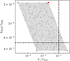 |
Fig. C.1. Trend of the accretion regime LBLR/LEdd as a function of Lγ/LEdd in the case of upper limits on both the optical and γ-rays. The red star is the chosen initial value, the gray points indicate the region spanned when the three quantities LBLR, LEdd, and Lγ vary. The gray stars represent the final values of the parameter simulation. The dotted black lines represent the separation limits for the accretion efficiency, respectively LBLR/LEdd ∼ 5 × 10⁻⁴ and Lγ/LEdd ∼ 0.1 (Ghisellini et al. 2011b; Sbarrato et al. 2012). In this case, LBLR varies between [1044,1046] erg ⋅ s−1, Lγ between [1045,1047] erg ⋅ s−1. |
Appendix D: Evaluating the reliability of statistical methods for handling censored data
In our study of PeVatron blazar candidates and comparison samples, we assessed the applicability of statistical methods that incorporate censored data, i.e., upper and/or lower limits (“left-” and “right-censored” data, respectively) into the analysis. Previous studies have utilized survival analysis techniques to handle such censored data effectively. Specifically, the Kaplan–Meier estimator is employed to estimate the survival function of a given quantity in a sample, accommodating both uncensored and censored observations. To compare properties across different samples, tests such as the logrank and Peto logrank are utilized, which include weighting schemes to account for censored data points (Feigelson & Nelson 1985; Lavalley et al. 1992; Padovani 1992; Homan et al. 2021; Baldi et al. 2022; Padovani et al. 2022b; Paiano et al. 2023).
We investigated both the logrank test and the Peto logrank test, the latter being reported to be less affected by differences in censoring patterns between samples (Feigelson & Nelson 1985; Padovani et al. 2022b; Paiano et al. 2023), and found that the results are highly sensitive to the rate of censored data and the sample size. To evaluate the suitability of these methodologies for our study, we conducted several analyses, especially covering cases where significant discrepancies were observed in Section 6. Below, we summarize the findings most pertinent to our study.
D.1. Experiment setup and findings
We utilized samples which list only measurements, such as the 5BZCat redshift, with a total of 2753 values, 4LAC-DR3 γ-ray luminosity (1846), and P17 black hole mass (47). We initially constructed comparison subsamples comprising only detections by randomly selecting values from the parent dataset. We generated multiple test subsamples with increasing sizes to evaluate the consistency of these subsamples with the original datasets. To do this, we employed the Kaplan–Meier estimator alongside the logrank and Peto logrank tests. As expected, these distributions remained compatible, regardless of the physical quantities tested, as illustrated in the left panels of Fig. D.1. In this way, we assessed and confirmed their comparability to the original datasets, and also validated the expected performance of both the logrank and Peto logrank tests.
Subsequently, we generated mock samples by introducing left-censored data. These mock samples were constructed to have the same size and distribution as the original dataset, with the only difference being that some measurements were flagged as ULs. This involved randomly selecting an increasing number of measurements and flagging them as ULs. We adopted the more extreme scenario of turning the measurements into upper limits, resulting in the lowest pvalues, as this represents the most conservative approach. We, then, applied survival analysis to compare these mock samples to the original sample, as shown in the right panels of the same Fig. D.1. Our findings revealed that the Peto logrank test is less biased by censoring patterns compared to the standard logrank test, as discussed in Feigelson & Nelson (1985). Consequently, we based our analysis on the Peto logrank test. However, the resulting pvalues, plotted against the number of ULs, showed increasing discrepancies as the fraction of limits grows, highlighting potential limitations in the test’s applicability.
As an additional test, we evaluated the reliability of this method as a function of the fraction of upper limits relative to the total sample size, considering different sample sizes equal to 20, 50, 100, 200. From the parent sample, we extracted two subsamples of the same size. One was kept unmodified, i.e., its values are the same as the original sample and considered as measurements. In the second subsample, a progressively larger number of them were flagged as UL. In this way, the second subsample includes both measurements and limits, but the overall distribution is identical to the parent sample by construction. We recorded the Peto logrank pvalues obtained over 100 realizations for each scenario and estimated their median. The results obtained using the 5BZCat redshift are shown in Fig. D.2. The Figure illustrates the median Peto logrank pvalues plotted against the percentage of ULs relative to the total sample size. The horizontal dashed-dotted and dashed lines indicate the 3σ and 5σ levels, respectively. This analysis demonstrated that, as the proportion of ULs increases, the pvalues tend to decrease, indicating a higher likelihood of running into Type I errors. Another finding is that increasing the sample size, while maintaining the same percentage of censored data, increased the likelihood of false positives. This occurs because a larger sample inherently includes more censored data.
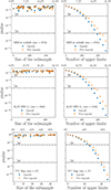 |
Fig. D.1. Redshift distribution of 5BZCat (top), the Lγ distribution of 4LAC-DR3 (middle) and the MBH distribution of P17 (bottom) are used to access the reliability of the statistical approaches. The left panels show the result of the logrank (blue points) and Peto logrank tests (orange squares) performed on the original population (only measurements) vs. comparison subsamples of progressively larger size, constructed by randomly selecting measured values from the parent dataset. The pvalue is shown as a function of the size of the selected subsample. The right panels show the result of the logrank (blue points) and Peto logrank (orange squares) tests performed on the parent populations (only measurements) vs. mock samples of the same size as the parent population, where a progressively larger number of values is flagged as censored data. The pvalue is shown as a function of the number of limits. In both panels, the upper axis indicates the percentage with respect to the total size of the sample (see Appendix D). |
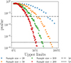 |
Fig. D.2. Peto logrank pvalues as a function of the number of upper limits (in percentage with respect to the total sample size). From the 5BZCat redshift sample, two subsamples of equal size were extracted: the first is kept unmodified (only measurements), in the second a progressively larger number of measurements were flagged as UL. In this way, the second subsample includes both measurements and censored data. The Peto logrank test was applied to subsamples of the same size at each step. The results for subsample size =20 in blue, 50 in orange, 100 in green, and 200 in red are shown by plotting, for each case, the median of the pvalues obtained over 100 realizations. |
D.2. Applicability in the context of our study
In the analysis presented in Section 6, three tests highlighted significant discrepancies ( ≳ 3σ) with the Peto logrank approach. These are marked with the symbol * in the rightmost column of Table A.3. Two of these tests involved only measurements or a small amount of censored data. Specifically, these included the comparison with S12 of the redshift, where the total sample sizes were 49 vs 162, with 6% censored data, and P1.4 GHz, with total sample sizes of 52 vs 74. These cases are similar to the simulations presented in Figures D.1 (bottom) and D.2 (orange, green, red), which demonstrated that when testing samples with little or no censored data, the Peto logrank test performs as expected and can therefore be regarded as reliable. They are also consistent with the corresponding A-D pvalues.
The third test compared the MBH distributions between the target sample and the P17 sample. The target sample consisted of 52 observations, approximately 38% of which were censored data, while the P17 sample comprised 47 measurements with no censored data. To assess the robustness of this result, we referred to simulations shown in Figures D.1 (bottom) and D.2 (orange). These simulations with sample sizes and an UL fraction closest to those of the observed pvalue 1.70 × 10⁻⁶ conservatively results in a pvalue of > 10−2. Thus, we expect the 38% UL of the MBH test against P17 to have underestimated its intrinsic pvalue by a factor of > 10−2 in the worst-case scenario. In other words, the UL-corrected pvalue is expected to be < 1.70 × 10⁻⁶/0.01 = 1.70 × 10⁻⁴, placing it at the third rank. Since the third rank Benjamini-Hochberg critical threshold is ∼2.8 × 10⁻⁴ and the UL-corrected pvalue is conservatively < 1.70 × 10⁻⁴, we conclude that the MBH test using P17 is significant at the ≳3σ level and may be attributable to an intrinsic difference between the tested samples.
Appendix E: Atlas of optical spectra
In this section, we show the new optical spectra acquired for this work in Fig.E.1 (see Table B.1 and Appendix B for all the details, also for the spectra that were already available in the literature and/or public archives).
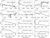 |
Fig. E.1. Newly acquired optical spectra for this work. The flux on the y-axis is in units [erg·cm−2·s−1 · Å−1], the wavelengths on the x-axis in [Å] (see Table B.1 and Appendix B for all the details). |
All Tables
List of candidate PeVatron blazars–neutrino hotspot associations from PAPER I and PAPER II.
Physical properties of the candidate PeVatron blazar sample estimated in this work.
All Figures
|
Fig. 1. Venn diagram showing the overlap between the three comparison samples S12 (Sbarrato et al. 2012), P17 (Paliya et al. 2017) and P21 (Paliya et al. 2021). |
| In the text | |
|
Fig. 2. LBLR/LEdd (accretion regime proxy) vs. Lγ/LEdd (power of the jet proxy) of the candidate PeVatron blazars (black). The three blue FSRQs (masquerading BL Lacs) TXS 0506+056, PKS 1424+240, and 5BZB J0630-2406 that were previously identified as promising neutrino-emitter blazar candidates are highlighted in cyan, lime, and magenta, respectively (see Sect. 6.3). As a comparison, the plot also shows the samples of S12, P17, and P21 (see Sect. 3.2). For P17, we plot the subsample with properties analyzed through optical spectroscopy. The arrows represent upper limits on either one or both of the shown quantities (see also Appendix C). The dotted gray lines represent the boundaries for the different accretion efficiencies, respectively LBLR/LEdd ∼ 5 × 10⁻⁴ and Lγ/LEdd ∼ 0.1 (Ghisellini et al. 2011b; Sbarrato et al. 2012). On the sides are the histograms of the corresponding quantities for all the samples, excluding all the upper limits. Here the black solid lines represent the median values for the candidate PeVatron blazars. |
| In the text | |
|
Fig. 3. Accretion regime LBLR/LEdd as a function of the radio power at 1.4 GHz, compared to the samples of (S12, P17, and P21 in the plot, Sbarrato et al. 2012; Paliya et al. 2017, 2021, see Sect. 3.2 for further details). For P17 we plot the subsample whose properties are analyzed through optical spectroscopy. The arrows indicate the upper limits on the optical luminosity. The three blue FSRQs (masquerading BL Lacs) TXS 0506+056, PKS 1424+240, and 5BZB J0630-2406 that were already identified as promising neutrino-emitter blazar candidates are highlighted in cyan, lime, and magenta, respectively (see Sect. 6.3). The dashed horizontal gray line represents the separation limits for the accretion efficiency LBLR/LEdd ∼ 5 × 10⁻⁴ (Ghisellini et al. 2011b; Sbarrato et al. 2012). Instead, the vertical dotted line is the threshold P1.4 GHz ∼ 1026 W ⋅ Hz−1 above which HERGs dominate over LERGs (Best & Heckman 2012; Padovani et al. 2019). On the sides are the normalized histograms of the corresponding quantities for the samples, excluding all the upper limits. Here, the black solid lines represent the median value for the candidate PeVatron blazars. |
| In the text | |
|
Fig. 4. Distribution of the redshift, black hole mass, disk luminosity, size of the broad line region and dusty torus, and γ-ray luminosity. The comparison samples are Sbarrato et al. (2012), Paliya et al. (2017, 2021) (S12, P17, P21, respectively), BZCat and 4LAC-DR3, with the exclusion of upper limits on the plotted quantity. The black solid lines correspond to the median value for the candidate PeVatron blazars. |
| In the text | |
|
Fig. C.1. Trend of the accretion regime LBLR/LEdd as a function of Lγ/LEdd in the case of upper limits on both the optical and γ-rays. The red star is the chosen initial value, the gray points indicate the region spanned when the three quantities LBLR, LEdd, and Lγ vary. The gray stars represent the final values of the parameter simulation. The dotted black lines represent the separation limits for the accretion efficiency, respectively LBLR/LEdd ∼ 5 × 10⁻⁴ and Lγ/LEdd ∼ 0.1 (Ghisellini et al. 2011b; Sbarrato et al. 2012). In this case, LBLR varies between [1044,1046] erg ⋅ s−1, Lγ between [1045,1047] erg ⋅ s−1. |
| In the text | |
|
Fig. D.1. Redshift distribution of 5BZCat (top), the Lγ distribution of 4LAC-DR3 (middle) and the MBH distribution of P17 (bottom) are used to access the reliability of the statistical approaches. The left panels show the result of the logrank (blue points) and Peto logrank tests (orange squares) performed on the original population (only measurements) vs. comparison subsamples of progressively larger size, constructed by randomly selecting measured values from the parent dataset. The pvalue is shown as a function of the size of the selected subsample. The right panels show the result of the logrank (blue points) and Peto logrank (orange squares) tests performed on the parent populations (only measurements) vs. mock samples of the same size as the parent population, where a progressively larger number of values is flagged as censored data. The pvalue is shown as a function of the number of limits. In both panels, the upper axis indicates the percentage with respect to the total size of the sample (see Appendix D). |
| In the text | |
|
Fig. D.2. Peto logrank pvalues as a function of the number of upper limits (in percentage with respect to the total sample size). From the 5BZCat redshift sample, two subsamples of equal size were extracted: the first is kept unmodified (only measurements), in the second a progressively larger number of measurements were flagged as UL. In this way, the second subsample includes both measurements and censored data. The Peto logrank test was applied to subsamples of the same size at each step. The results for subsample size =20 in blue, 50 in orange, 100 in green, and 200 in red are shown by plotting, for each case, the median of the pvalues obtained over 100 realizations. |
| In the text | |
|
Fig. E.1. Newly acquired optical spectra for this work. The flux on the y-axis is in units [erg·cm−2·s−1 · Å−1], the wavelengths on the x-axis in [Å] (see Table B.1 and Appendix B for all the details). |
| In the text | |
Current usage metrics show cumulative count of Article Views (full-text article views including HTML views, PDF and ePub downloads, according to the available data) and Abstracts Views on Vision4Press platform.
Data correspond to usage on the plateform after 2015. The current usage metrics is available 48-96 hours after online publication and is updated daily on week days.
Initial download of the metrics may take a while.