| Issue |
A&A
Volume 700, August 2025
|
|
|---|---|---|
| Article Number | A12 | |
| Number of page(s) | 26 | |
| Section | Extragalactic astronomy | |
| DOI | https://doi.org/10.1051/0004-6361/202451860 | |
| Published online | 01 August 2025 | |
Narrow-line AGN selection in CEERS: Spectroscopic selection, physical properties, and X-ray and radio analysis
1
Dipartimento di Fisica e Astronomia, Università di Bologna, Via Gobetti 93/2, I-40129 Bologna, Italy
2
INAF –Osservatorio di Astrofisica e Scienza dello Spazio di Bologna, Via Gobetti 93/3, I-40129 Bologna, Italy
3
Kavli Institute for Cosmology, University of Cambridge, Madingley Road, Cambridge CB30HA, UK
4
Cavendish Laboratory, University of Cambridge, 19 JJ Thomson Avenue, Cambridge CB3 0HE, UK
5
Department of Physics and Astronomy, University College London, Gower Street, London WC1E6BT, UK
6
Dipartimento di Fisica e Astronomia, Università di Firenze, Via G. Sansone 1, 50019 Sesto Fiorentino, Firenze, Italy
7
INAF – Osservatorio Astrofisico di Arcetri, Largo Enrico Fermi 5, 50125 Firenze, Italy
⋆ Corresponding author: This email address is being protected from spambots. You need JavaScript enabled to view it.
Received:
11
August
2024
Accepted:
7
February
2025
Abstract
The transformative era opened by the James Webb Space Telescope (JWST) on the high-z Universe allows us to investigate the early stages of supermassive black hole (SMBH) evolution, with the first results showing a greater than expected number of active galactic nuclei (AGNs) at very early times. In this work, we spectroscopically select narrow-line AGNs (NLAGNs) among the ∼300 publicly available medium-resolution spectra of the Cosmic Evolution Early Release Science Survey (CEERS). Using both traditional and newly identified emission line NLAGN diagnostics diagrams, we identified 52 NLAGNs at 2 ≲ z ≲ 9, on which we performed a detailed multiwavelength analysis. We also identified four new z ≲ 2 broad-line AGNs (BLAGNs), in addition to the eight previously reported z > 4.5 BLAGNs. We found that the traditional BPT diagnostic diagrams are not suited to identifying high-z AGNs, while most of the high-z NLAGN were selected using the recently proposed AGN diagnostic diagrams based on the [O III] λ4363 auroral line or high-ionization emission lines. We compared the emission line velocity dispersion and the obscuration levels of the sample of NLAGNs with those of the parent sample without finding significant differences between the two distributions, suggesting a population of AGNs heavily buried and not significantly impacting the host galaxies’ physical properties, as was further confirmed by spectral energy distribution fitting. The bolometric luminosities of the high-z NLAGNs selected in this work are ∼1.5 dex below the ones sampled by surveys before JWST, potentially explaining the weak impact of these AGNs. Finally, we investigated the X-ray properties of the selected NLAGNs and of the sample of high-z BLAGNs. We found that all but four NLAGNs are undetected in the deep X-ray image of the field, as well as all the high-z BLAGNs. We did not obtain a detection even by stacking the undetected sources, resulting in an X-ray weakness of ∼1 − 2 dex from what was expected based on their bolometric luminosities. To discriminate between a heavily obscured AGN scenario or an intrinsic X-ray weakness of these sources, we performed a radio (1.4GHz) stacking analysis, which did not reveal any detection and left open the questions about the origin of the X-ray weakness.
Key words: galaxies: active / galaxies: high-redshift / galaxies: ISM
© The Authors 2025
 Open Access article, published by EDP Sciences, under the terms of the Creative Commons Attribution License (https://creativecommons.org/licenses/by/4.0), which permits unrestricted use, distribution, and reproduction in any medium, provided the original work is properly cited.
This article is published in open access under the Subscribe to Open model. This email address is being protected from spambots. You need JavaScript enabled to view it. to support open access publication.
1. Introduction
Thanks to the successful launch of the James Webb Space Telescope (JWST; Gardner et al. 2023; Rigby et al. 2023), we are now able to investigate with a high resolution and an unprecedented sensitivity both the photometric and spectroscopic properties of galaxies up to z ∼ 14 (Carniani et al. 2024; Curtis-Lake et al. 2023; Robertson et al. 2023). Within this context, recent studies, exploiting both spectroscopic and imaging data from JWST, have revealed a large population of active galactic nuclei (AGNs) at high redshift (Kocevski et al. 2023; Übler et al. 2023, 2024; Matthee et al. 2024; Maiolino et al. 2024a,b; Greene et al. 2024; Bogdán et al. 2023; Goulding et al. 2023; Kokorev et al. 2023; Furtak et al. 2024; Juodžbalis et al. 2024a; Scholtz et al. 2025; Chisholm et al. 2024), providing a unique opportunity to study the properties of supermassive black hole (SMBH) and AGN-galaxy coevolution since very early times.
Different works, selecting AGNs at high-z using JWST NIR and MIR photometry, have shown that the AGN population at z > 3 is larger than previously expected and that it is probably dominated by obscured or even heavily obscured sources, as is predicted by some
coevolutional models Hopkins et al. (2008), Hickox & Alexander (2018). Yang et al. (2023), taking advantage of the JWST-MIRI photometry of the Cosmic Evolution
Early Release Science Survey (CEERS; Finkelstein et al. 2022), investigated the AGN population using spectral energy distribution (SED) modeling and found a black-hole accretion rate density (BHARD) at z > 3 ∼ 0.5 dex higher than what was expected from previous X-ray AGN studies (Vito et al. 2016, 2018). Also, Lyu et al. (2024), performing a similar analysis using the JWST/MIRI data of the SMILES survey, selected a remarkable fraction of AGNs among the MIRI-detected sources (∼7%) and found a statistically significant increase in the obscured AGN fraction with redshift, as had previously been found in other works (Signorini et al. 2023; Gilli et al. 2022; Buchner et al. 2015; Aird et al. 2015).
The existence of a larger-than-expected AGN population at z > 4 has also been shown by spectroscopic studies. For example, Maiolino et al. (2024b) and Harikane et al. (2023), by selecting broad-line AGNs (BLAGNs, or type I) among JWST/NIRSpec spectra, found a significant AGN excess at z > 4 with respect to the AGN luminosity functions derived using X-ray data (Giallongo et al. 2019).
JWST data not only allow for the identification of a higher fraction of AGNs at high-z but also show some new and unexpected features in this early population of SMBHs. Studies have revealed that early SMBHs tend to be overmassive relative to the host galaxy stellar mass, when compared with the local AGN distribution (Maiolino et al. 2024b; Bogdán et al. 2023; Furtak et al. 2024; Juodžbalis et al. 2024a), suggesting that the early stages of the coevolution between the SMBH and the host galaxy can be dominated by SMBH growth. This could further suggest that the preferred driving channel for the SMBH formation is the so-called “direct collapse black hole” scenario, together with (or alternatively) episodes of super-Eddington accretion (Scholtz et al. 2024a).
Another remarkable feature of high-z newly discovered AGNs is that they seem to be X-ray-weak compared to the low-redshift AGN population. X-rays have traditionally been used to select AGNs because at typical AGN X-ray luminosities (log LX ≥ 42), the level of contamination by stellar processes is low, allowing for a generally pure AGN selection. However, even if X-ray photons are able to penetrate through dense environments, they are almost completely absorbed at Compton-thick (CTK) hydrogen column densities (log(NH/cm−2) ≥ 24), making the X-ray identification of heavily obscured AGNs challenging (Vignali et al. 2015; Lanzuisi et al. 2018; Goulding et al. 2023; Maiolino et al. 2025).
Specifically, most of the newly selected AGNs, including BLAGNs, lack any X-ray emission (Maiolino et al. 2025; Yue et al. 2024), even if they are located in fields covered by some of the deepest extragalactic X-ray observations ever performed. Given the very few exceptions (Goulding et al. 2023; Kovács et al. 2024; Maiolino et al. 2025) of X-ray AGN detections in the early Universe, it is possible that the X-ray weakness could be due to intrinsic properties of high-z AGNs, as has also been suggested for some low-z AGNs (Simmonds et al. 2018; Zhang et al. 2024). In this view, AGNs can be characterized by a different accretion-disk and/or X-ray corona structure that can determine, for example, a larger ratio of the optical to X-ray emission (αOX) due to a much lower efficiency of the corona in producing X-ray photons, or simply a lack of corona (Proga 2005). Recently, Maiolino et al. (2025), analyzing the lack of X-ray emission in a large sample of high-z sources unambiguously identified as AGNs, suggested that their X-ray weakness could also be ascribed to the presence, in the inner region of the AGNs, of a spherical distribution of clouds with CTK column densities and very low dust content, such as the broad-line region (BLR) clouds. In this hypothesis, high-z BLAGNs do not need to be characterized by any kind of intrinsic X-ray weakness, as their lack of X-ray emission would simply be caused by the inner CTK BLR gas.
JWST spectroscopy can give us information on the nature of the observed sources, allowing us to identify and investigate not only the population of BLAGNs, which is probably only the tip of the iceberg of the entire AGN census, but also the vast and hidden population of narrow-line AGNs (NLAGNs, also called type II). An additional significant difference between high-z and low-z AGNs lies in the remarkably different physical environments constituted by their host galaxies. Indeed, early galaxies are systematically more metal-poor and characterized by younger stellar populations (Curti et al. 2023) that increase their ionization parameters in the ISM (log U; Cameron et al. 2023; Curti et al. 2023). These two effects have a significant impact on the selection of NLAGNs, traditionally based on optical emission-line diagnostic diagrams, because the lower metallicities and the larger log U make star-forming galaxies (SFGs) and AGNs move toward each other and eventually overlap on the traditional diagnostic diagrams (Übler et al. 2023; Kocevski et al. 2023; Maiolino et al. 2024b; Scholtz et al. 2025; Mazzolari et al. 2024).
However, the identification of the elusive population of NLAGNs is crucial in order to have a complete census of the AGN population, especially at high-z, and to build up statistical AGN samples that can solve the problems in AGN identification and properties at high-z. So far, a systematic search for NLAGNs at z > 3 has only been attempted by a few works. In Scholtz et al. (2025), the authors selected 42 NLAGNs among ∼200 medium-resolution (MR) spectra of the JADES survey (Eisenstein et al. 2023; Bunker et al. 2023). In particular, they used JADES spectra to select NLAGN through a series of rest-frame optical, rest-frame UV diagnostic diagrams, and by exploiting the detection of high-ionization emission lines, which usually require an AGN as a photoionizing source. The selected sample allowed the authors to investigate the population of AGNs up to z ∼ 9, down to bolometric luminosities of log Lbol ∼ 42 and host galaxy stellar masses of 107 M⊙, vastly expanding the region of the parameter space populated by these objects at early times.
In this work, we perform a similar analysis, investigating the NLAGN population hidden among the sample of MR spectra collected in the CEERS survey. The paper is organized as follows. In Sect. 2, we present the data and the sample of spectra analyzed throughout this work and the techniques involved in the subsequent analysis: emission line fitting, spectral stacking, SED-fitting, and X-ray and radio stacking. In Sect. 3, we describe the different emission line diagnostic diagrams involved in the NLAGN selection and the results of the selection. Then, in Sect. 4, we discuss the physical properties of the selected NLAGNs: the AGN prevalence (Sect. 4.4), the distribution in velocity dispersion and obscuration (Sect. 4.5, Sect. 4.6), the bolometric luminosities (Sect. 4.7), the host galaxies properties (Sect. 4.8), and finally, in Sect. 4.9 and Sect. 4.10, the X-ray and radio analysis, respectively. We assume a flat ΛCDM Universe with H0 = 70 km s−1 Mpc−1, Ωm = 0.3, and ΩΛ = 0.7.
2. Data and methods
2.1. CEERS observational data
We used publicly available MR JWST NIRSpec (Jakobsen et al. 2022) Micro-Shutter Assembly (MSA; Ferruit et al. 2022) data from the CEERS program (Program ID:1345, Finkelstein et al. 2022). The CEERS NIRSpec observations consist of six pointings in the ‘Extended Groth Strip’ field (EGS; Rhodes et al. 2000; Davis et al. 2007), all of which utilized the three grating and filter combination of G140M/F100LP, G235M/F170LP, and G395M/F290LP. This provided a spectral resolution of R ∼1000 over the wavelength range of approximately 1–5 μm (Jakobsen et al. 2022). Each grating and filter combination was observed for a total of 3107s for each pointing.
In particular, we considered the 313 spectra reduced and published by the CEERS collaboration in their latest data release, DR-0.71. The data reduction was performed by the CEERS collaboration using the JWST Calibration Pipeline version 1.8.5 (Bushouse et al. 2022), using the CRDS context “jwst_1029.pmap.” The spectra were reduced using standard processing pipeline parameters, with some specific deviation in particular regarding the “jump” parameters and the so-called “snowball” corrections. Nodded background subtraction was employed. The pipeline was instructed that all targets should be treated as point sources, determining each 1D spectrum to be extracted from the 2D spectral data file over a specified range of pixels in the cross-dispersion direction. Extraction apertures on the 2D spectra were determined for each object by interactive visual inspection and were specified explicitly for the pipeline step “extract_1d.” Most faint galaxies are compact, and the extraction apertures adopted for nearly all objects have heights ranging from 3 to 6 pixels (scale = 0.10 arcsec/pixel), with a median value of 4 pixels. The default pipeline path-loss correction was employed. This calibration is based primarily on pre-flight modeling, assuming the targets are point sources and determining these corrections to be incomplete for significantly extended sources, but this is not the case for the large majority of the targets. Flux calibration uses the default reference files for the adopted CRDS context.
For this work, we used the spectra with the three single grating spectra combined together. The data from the individual MR gratings were resampled to a common wavelength vector in the overlapping regions, adopting the wavelength grating that in the overlap region has the worst spectral resolution. The flux values in the overlap regions are the average of the individual grating values weighted by the flux errors, excluding pixels affected by masked artefacts.
After a careful visual inspection of the 313 single MR spectra available, we were able to attribute a secure redshift to 217 sources, constituting our parent sample throughout this work.
Harikane et al. (2023) already investigated a limited sample of these spectra (i.e., only those at z > 3.8) to look for BLAGN, selecting 10 AGNs at z = 4.015 − 6.936 (2 of which are marked only as candidates) whose broad component is only seen in the permitted Hα or Hβ lines and not in the forbidden [O III] λ5007 line. In the rest of the paper we mark the 8 most reliable BLAGNs selected in Harikane et al. (2023) as the sample of high-z BLAGNs.
2.2. Emission line fitting
The NLAGN selection performed in this work is based on emission line diagnostics diagrams, where the AGN selection is provided by demarcation lines taken from the literature or by comparing the distribution of the sources with photoionization models, following the procedure done in Scholtz et al. (2025)2.
We used a modified version of the publicly available code QubeSpec (Scholtz et al. 2025; D’Eugenio et al. 2025) to fit the spectra of the sources. We fit the emission lines considering only small wavelength ranges around the single (or group of) emission lines (∼ 500 Å), with each emission line fit using a single Gaussian component. The continuum was fit with a power law model, and in most of the spectra it was not detected. This approach for the fit of the continuum is sufficient for describing a narrow continuum range around an emission line of interest, and we found no instances of a strong continuum that required more sophisticated (e.g., stellar emission) modeling. QubeSpec uses a Bayesian approach, which requires defining prior probability distributions for each model parameter. In our fit, we assume log-uniform priors for the peak of the Gaussian describing each line and also for the continuum normalization. The prior on the lines full-width half maximum (FWHMs) is set to a uniform distribution spanning from the minimum resolution of the NIRSpec/MSA (∼200 km/s) up to a maximum of 700 km/s. For the fit of the high-z BLAGNs identified in Harikane et al. (2023) we also include in the fit a broad component in the Hα (with a FWHM uniform prior between 900 − 5000 km/s) to carefully disentangle the broad Hα emission from the narrow one, which is the only component used in the diagnostic diagrams. The prior on the redshift is a normal distribution centered on the redshift obtained from the visual inspection with a standard deviation of 100 km/s.
To estimate the posterior probability distribution of all these parameters, we use a Markov chain Monte Carlo integrator (emcee; Foreman-Mackey et al. 2013).
To address the NLAGN selection, we performed a fit of the following rest-frame optical and UV emission line blocks:
-
Hα + [N II] λλ6548,83 + [S II] λλ6716,31
-
[O I] λ6300
-
Hβ + [O III] λλ4959,5008 + He II λ4686
-
Hγ + [O III] λ4363
-
[O II] λλ3726,29 + [Ne III] λ3869
-
[Ne V] λ3426
-
[Ne IV] λλ2422,24
-
C III] λλ1907,10
-
[O III] λλ1660,66 + He II λ1640 +C IV λλ 1548,51
-
N IV] λλ1483,86
-
Lyα + N V λ1240.
For the components of the [O III] λλ4959,5008 and [N II] λλ6548,84 doublets, we fixed the ratios between the two components to be 1:3 given by the relative Einstein coefficients of the two transitions. Given the resolution of the NIRSpec MR spectra, we fit the [O II] λλ3726,29, [Ne IV] λλ2422,24, C IV λλ 1548,51, [O III] λλ1660,66, C III] λλ1907,10, and N IV] λλ1483,86 doublets as single Gaussians, centered at the mean wavelength between the two components. The signal-to-noise ratio (S/N) of each line was evaluated considering the same equations reported in Mignoli et al. (2019) and Lenz & Ayres (1992):
 (1)
(1)
where Δλ is the sampling interval of the spectrum, (S/N)0 is the peak S/N (i.e., (S/N)0 = f0/σ0, where f0, σ0 are the flux density and the noise level at the central pixel), and C is a proportionality constant whose values are reported in Table 1 of Lenz & Ayres (1992). We also checked the S/N using the following equation:
 (2)
(2)
where fi and σi are the flux densities and associated errors for flux bins falling inside the Gaussian profile of the fit, and we found results consistent with those derived from Eq. (1). We required at least S/N > 5 for the detection. Then, we visually inspected all the detected lines to exclude any possible false detection. In case of undetection, we derived the upper limit to the flux of each line as 3σ errors (with σ the error returned by QubeSpec).
While fitting the Hα line, we found 4 sources at z ≤ 2 for which the residuals from the narrow-line-only fit were too large, and a broad component was required. These sources were not selected as in Harikane et al. (2023) because in that work the authors investigated only sources at z > 3.8. We identify these sources as new BLAGNs at low-z; their spectra are presented in Appendix A. In fitting all the BLAGNs, we did not find any significant broad component either in the Hβ or in the [O III] λ5007 lines.
2.3. Spectral stacking
Once the final sample of 52 NLAGNs has been selected, to get the average emission line properties of the SFGs and NLAGN samples, we stacked the MR spectra for each of the emission line complexes investigated in this work. The spectral stacking was performed by normalizing all the NLAGN and SFG spectra by the peak flux of the [O III] λ5007 line in order not to be biased toward the brightest objects. The [O III] λ5007 line is the most common and well-detected line among the CEERS MR spectra, but is not available in 8 AGNs and in 14 SFG spectra because for these sources the line falls into a detector gap. Therefore, we excluded them from the stacking. We shifted all the spectra to the rest frame, and then we resampled each of the spectra to a uniform and common wavelength grid, given that the three components of each spectrum (corresponding to the three different gratings) have different resolutions and wavelength bins. The new and uniform wavelength grid was defined, for each line complex, by the wavelength bin allowing for the best spectral resolution among the different resolutions of the spectra involved in the stacking of the line(s). We checked that the results do not significantly change, taking the wavelength bin corresponding to the worst spectral resolution among the spectra. Before stacking the spectra, we also fit and subtracted the continuum from the rest-frame rebinned spectra.
We finally opted for spectral stacking involving a bootstrap procedure, given the number of sources involved. The stacked spectrum and uncertainties of each spectral bin were derived taking the median and standard deviation of 250 bootstrap realizations of the input spectra. The resulting spectra from the stacking of all NLAGNs and SFGs are presented in Fig. 1.
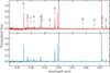 |
Fig. 1. Stacked spectra of the final sample of NLAGNs (red) and non-AGNs (blue) derived in the manner described in Sect. 2.3. We also marked the positions of some relevant lines. |
2.4. SED fitting
To investigate the physical properties of the host galaxies of the selected NLAGNs and to compare them with the properties of the parent sample, we performed a SED fitting analysis using CIGALE (Boquien et al. 2019). Starting from the 217 spectra of the MR sample with a secure redshift, we first crossmatch the target coordinates with the HST+JWST publicly available photometric catalog of the CEERS field reported in the DJA archive3. Considering a 0.5″matching radius we found 117 counterparts. This catalog includes seven HST bands (F435W, F606W, F814W, F105W, F125W, F140W, F160W) and ten JWST/NIRCam and MIRI bands (F115W, F150W, 182M, F200W, 210M, F277W, F356W, F410M, F444W, F770W). Since not the whole CEERS MR sample is covered by JWST imaging, we also crossmatched the remaining sources with the 3D-HST multiwavelength catalog (Momcheva et al. 2016; Skelton et al. 2014), covering the EGS field and using the same crossmatching radius to avoid false matches. We found 93 additional counterparts, bringing the total number of sources with an associated optical/NIR photometry to 210. For the remaining seven spectra, we did not find a counterpart closer than 0.5″, but their counterparts are returned when we considered a larger crossmatching radius (0.5″ < r < 1.2″). For sources detected in the JWST+HST catalog, we did not consider the additional photometry of the 3D-HST catalog since most of these sources are undetected in photometric bands bluer than the HST bands (being at high-z), while the photometry at longer wavelengths than HST bands is already covered by JWST (the deepest in the near and mid-infrared).
The SED fitting was performed considering two different parameter grids, reported in Appendix B, one for sources at z < 3 and the other for sources at z > 3. We used delayed star formation history (SFH) models for both redshift groups because they are able to reproduce both early-type and late-type galaxies, with an additional term that allows for a recent (and constant) variation in the star formation rate (SFR) that can be in the burst or in the quench phase. We adopted stellar templates from Bruzual & Charlot (2003), and a Chabrier initial mass function (Chabrier 2003). We also include the nebular emission module that is extremely important to account for the contribution of emission lines in the broad-band photometry (Schaerer & de Barros 2012; Salvato et al. 2019), in particular for the low-mass and high-z regimes, where emission lines can account for a consistent fraction of the wideband photometric flux. This module is computed by CIGALE based on a grid of user-provided parameters and in a self-consistent manner using a grid of Cloudy photoionization calculations Ferland et al. (2013). For the attenuation of the stellar continuum emission, we considered the dustatt_modified_CF00 module (Charlot & Fall 2000), which allows different attenuations for the young and old stellar populations. We also include dust emission in the IR following the empirical templates of Dale et al. (2014). The main differences in the z > 3 grid with respect to the low-z one consist in the larger parameter space explored for the possible final starburst state of high-z galaxies and in the lower metallicities and higher ionization parameters allowed in the stellar and nebular modules, according with recent JWST results (Endsley et al. 2024; Tang et al. 2023). Indeed, SFGs at high-z are observed to be more frequent in a bursty SF regime (Faisst et al. 2020; Dressler et al. 2023; Looser et al. 2025) and also, the gas metallicities are generally 0.5–1 dex lower than in the local Universe (Curti et al. 2024; Nakajima et al. 2023).
For sources classified as AGNs based on our NLAGN selection, as well as the BLAGNs selected in Harikane et al. (2023), we included AGN modules in the SED fitting to account for the AGN emission. We employed the skirtor2016 module introduced in Yang et al. (2020), which is widely used in the community and has demonstrated reliability in studying various aspects of AGN (e.g., Mountrichas et al. 2022; López et al. 2023; Yang et al. 2023). The SED produced by the AGN combines emissions from the accretion disk, torus, and polar dust. The accretion disk, responsible for the UV-optical emission at the central region, is parameterized according to Schartmann et al. (2005), with a typical delta value of −0.36. Photons from the accretion disk can be obscured and scattered by dust in the vicinity, within the torus and/or in the polar direction. Specifically, for the torus, the skirtor2016 module employs a clumpy two-phase model (Stalevski et al. 2016), based on the 3D radiative-transfer code SKIRT (Baes et al. 2011; Camps & Baes 2015). As our photometry does not cover the restframe mid-IR, we fixed the optical depth at 9.7 μm at τ = 3. For the polar dust component, we used the Small Magellanic Cloud (SMC) extinction curve, recommended due to its preference in AGN observations (e.g., Bongiorno et al. 2012). The extinction amplitude, parameterized as E(B − V), is a user-defined free parameter for which we chose a typical value of E(B − V) = 0.04. Emission from the polar dust maintains energy conservation, assuming isotropic emission and a “gray body” model (Casey 2012). Finally, we allowed inclination values from 50 to 80 degrees and varied the AGN fraction (defined as the ratio between the AGN luminosity and the host galaxy luminosity between 0.15 and 2 microns) from 0.1 (weak AGN contamination) to 0.7 (dominant AGN emission).
2.5. X-ray and radio stacking
To investigate the multiwavelength properties of the CEERS NLAGNs selected using the diagnostic diagrams, we looked at their counterparts in the X-rays and Radio images of the EGS field.
The Chandra AEGIS-XD field is the third deepest X-ray field ever performed, with an exposure that reaches ∼800 ks. The X-ray observations and the related X-ray catalog are described in Nandra et al. (2015). The X-ray catalog contains 937 X-ray sources, and 553 of these sources (those with enough photon counts) also have an X-ray spectral analysis performed by Buchner et al. (2015). By crossmatching the CEERS MR catalog with the X-ray catalog, we found seven matches, involving sources at 0.5 < z < 3. The X-ray spectral analysis classified two of these sources as galaxies (CEERS-3060, CEERS-3051), the other 5 (CEERS-2919, CEERS-2808, CEERS-2904, CEERS-2989, CEERS-2900) as AGN. In particular, CEERS-2904, CEERS-2989, and CEERS-2919 are part of the new low-redshift BLAGN sample presented in Appendix A.
Four out of the five X-ray AGNs were selected as NLAGNs by our spectroscopic selection, as we are going to present in Sect. 3. However, none of the other 48 NLAGNs selected show any indication of X-ray emission. Therefore, we decided to perform an X-ray stacking analysis of the NLAGNs not X-ray detected using the publicly available code CSTACK v4.5 Miyaji & Griffiths (2008). For each target, CSTACK provides the net (background-subtracted) count rate in the soft (0.5–2 keV) and hard (2–8 keV) bands using all the observations from the AEGIS-XD survey and the associated exposure maps. Since the survey is a mosaic, multiple observations at different off-axis angles can cover the same position. Due to the variation in the Chandra PSF with the off-axis angle, for each observation of an object, CSTACK defines a circular source extraction region with the size determined by the 90% encircled counts fraction radius (r90) (with a minimum of 1″), to optimize the S/N of the stacked signals. We set the background region for each source to be a 30 × 30 arcsec2 area centered on the object, excluding the region around the object used to compute the net counts. Moreover, the code excludes the photon counts of the background circular regions around all the detected X-ray sources, with radii that depend on the net counts of the X-ray source. We derived the count rates in the soft band (0.5–2 keV, SB), the band for which the detector is most sensitive and can, therefore, provide tighter constraints on the X-ray analysis. Then we converted the count rates into fluxes assuming an X-ray power spectrum with an intrinsic spectral index Γ = 1.9 and using the Chandra tool PIMMS4.
The field targeted by the CEERS survey is also covered by 1.4 GHz observations, the AEGIS20 described in Ivison et al. (2007). This radio survey was performed in 2006 with the Very Large Array (VLA) over an area of ∼0.75 deg2 and reaching, in the central region, a rms of ∼10 μJy. The resulting radio catalog (Ivison et al. 2007) contains 1123 individual radio sources, of which only two are part of the CEERS MR sample, CEERS-2900 and CEERS-3129, the first (that is also X-ray detected) showing the typical morphology of a radio-loud AGN. Both these sources were also identified as AGNs by our selection, but none of the other NLAGNs have any radio counterparts. Therefore, we performed a radio stacking analysis to investigate the radio statistical properties of the NLAGN population below the survey detection threshold. We applied a pixel-by-pixel median stacking, taking 30 × 30 arcsec2 cutouts around the sources we wanted to stack. This method was proved (White et al. 2007) to be more robust (compared to the mean stacking, for example) toward systematic effects (i.e., confusion) and also less affected by possible high-flux density contaminants. Since the CEERS survey covers only a very small region of the radio image on which the rms is almost uniform, we did not weigh each radio cutout for the corresponding noise value in the stacking procedure. We also estimated the final rms of the stacking images using a median absolute deviation procedure, following Keller et al. (2024).
3. Results
Here, we present the result of the NLAGN selection performed on the sample of the 217 MR CEERS spectra with a secure redshift identification. The NLAGN selection was performed using emission line diagnostic diagrams.
In all the diagrams, we plot both the observed data points and also the line ratios derived from the photoionization models described in Feltre et al. (2016) and Gutkin et al. (2016). These models were computed using the Cloudy code (Ferland et al. 2013) for SFG and AGN NL regions and for various gas metallicities, ionization parameters, dust content, and ISM densities, and considering a wide range of the parameters space (for the full grid of values covered by the parameter space we refer to Table 1 in Feltre et al. 2016). To allow for a sufficiently comprehensive coverage of the SFG models but to avoid physical conditions rarely (or never) found in the general populations of SFG in the local or high-z Universe, we applied to these models the same cut in the parameter space as presented and discussed in Scholtz et al. (2025). In particular, we selected all models with metallicities between 0.001 and 0.02 (corresponding to 0.06–1.3 solar) and a dust-to-metal mass ratio of 0.3, which is intermediate between the range observed in the most metal-poor absorbers (Konstantopoulou et al. 2023) and the Milky-Way value of 0.45. We consider all models with carbon to oxygen abundance ratio in the range 0.38–1.00 solar to describe a variety of different or less common star formation grids. Through the work, photoionization models for AGN and SFG will be shown in red and in blue, respectively. We also mark with distinctive colors the seven sources that are X-ray detected (gold), the two radio-detected sources (green), and the eight sources that were selected as BLAGNs at z > 4.5 by Harikane et al. (2023) (red). In each diagnostic diagram, the sources with magenta edges are those selected as NLAGN in that specific diagnostic.
It is worth noting that the line fluxes involved in the diagnostic diagrams described in the next Sections are not corrected for the effect of dust. This is because we are always considering ratios between lines close in wavelength to each other, hence subjected to almost the same reddening, making the ratio insensible to the presence of dust. The few exceptions are discussed and justified. The acronyms used for the line ratios are reported in Table 1.
Definitions of line ratios adopted throughout the paper.
3.1. Optical diagnostics
In Fig. 2, we show the traditional BPT diagram (Baldwin et al. 1981), the R3S2 (also called VO87), and the R3O1 (Veilleux & Osterbrock 1987) diagnostics diagrams based on the R3-N2, R3-S2, and R3-O1 line ratios, respectively. The traditional demarcation lines between SFG and AGN provided by Kauffmann et al. (2003) and Kewley et al. (2001) already proved to be way less effective in selecting high-z AGNs compared to the local Universe (Scholtz et al. 2025; Übler et al. 2023; Maiolino et al. 2024b). Indeed, the lower metallicities of high-z sources make [N II] (but also [S II] ) emission lines fainter, shifting the objects (AGN included) toward the left part of the BPT diagram. At the same time, the higher ionization parameter of the high-z SFG (Cameron et al. 2023; Sanders et al. 2023; Topping et al. 2024), due to, on average, the presence of younger stars and lower metallicities compared to the local Universe, moves the SFG toward higher R3 ratios, generating a large overlap between AGN and SFGs. Therefore, in the R3N2 and R3S2 diagnostics, we used the conservative demarcation lines provided in Scholtz et al. (2025), derived considering the distribution of the photoionization models of Gutkin et al. (2016), Feltre et al. (2016) and Nakajima & Maiolino (2022).
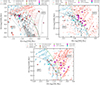 |
Fig. 2. Left: R3N2 diagnostic diagram (also called BPT). The gray points represent the parent sample of galaxies analyzed in this work. Gold, green and red colors are used, respectively, for X-ray detected sources, radio-detected sources, and the high-z BLAGNs reported in Harikane et al. (2023). The NLAGNs selected using this diagram are marked with magenta edges. In magenta and cyan, we show the line ratios derived from the stacked spectra of all the selected NLAGN (52 sources) and non-AGN sources. The dashed lines refer to three different demarcation lines, as labeled, the one in green is the more conservative demarcation line derived in Scholtz et al. (2025). The shaded blue and red area represents the regions covered by the SFG and AGN photoionization models computed in Gutkin et al. (2016) and Feltre et al. (2016). The gray contours mark the distribution of SDSS sources (taken from SDSS DR7; Abazajian et al. 2009). In the lower-right corner are reported the median errors of the sample. Right: R3S2 diagnostic diagram (also called VO87) with the demarcation line originally presented in Kewley et al. (2001) (in black) and the new (more conservative) demarcation derived in Scholtz et al. (2025). Bottom: R3O1 diagnostic diagram with the demarcation line presented in Kewley et al. (2001) (dashed black line) and the new one derived in this work (solid green line). |
Since the R3O1 diagnostic diagram was not included in the analysis of Scholtz et al. (2025), we followed the same fitting method to the photoionization models to find more conservative demarcation lines with respect to those presented in Kewley et al. (2001). We derived the following dividing line between the AGN and SFG population:
 (3)
(3)
As it is possible to see from the three plots, none of the BLAGNs at high-z are in the AGN region of the three diagnostics, based on the new demarcation lines, and only one would be selected considering the traditional demarcation lines in the R3S2 and R3O1 diagrams (is the same source, CEERS-1665).
The five AGNs selected with the R3N2 diagram are all at z < 2.9. Three of them are X-ray-detected AGNs (one is also radio-detected, i.e., CEERS-2900), and one is another radio-detected source (CEERS-3129). It is worth noting that even the X-ray source at the highest redshift (i.e., CEERS-2808 at z = 3.38), does not fall in the pure-AGN region of this diagnostic diagram.
The R3S2 diagnostic diagram appears effective in selecting AGN also at a higher redshift compared to the BPT. The new demarcation line provided in Scholtz et al. (2025) partially overlaps with the traditional one proposed in Kewley et al. (2001). In this case, we select 21 AGNs, six of which at z > 3, one at z = 5.27. None of the BLAGNs is selected as AGN based on this diagnostic, while three X-ray sources and the two radio sources are confirmed as AGN also in this diagnostic.
Also the R3O1 diagnostic diagram is more effective in identifying NLAGN compared to the R3N2. In this diagram, we select 12 AGNs, 7 at z < 3 (including 2 X-ray sources), and 5 at z > 3, one of these at z ∼ 6. We further discuss the effectiveness of this diagnostic and of the R3S2 in Sect. 4.1.
In Fig. 3, we show the diagnostic based on the He2 versus N2 lines ratio. In this case, the demarcation line is the original one provided by Shirazi & Brinchmann (2012), which still holds even at high-z, as also reported in Dors et al. (2024) and Tozzi et al. (2023). Overall, we detect He II λ4686 in seven sources: all except one of these are classified as AGN. None of the CEERS BLAGNs show detection of the He II λ4686 line. In this diagnostic, there are also five sources that are selected as AGN only based on the N2 ratio.
The last diagnostics exploiting rest-frame optical lines are the two diagnostics based on the O3Hg ratio and proposed in Mazzolari et al. (2024). Hereafter, we refer with M1 to the O3Hg versus O32 diagnostic diagram and with M2 to the O3Hg versus Ne3O2 diagram. These diagnostics proved to be effective in selecting those AGN characterized by high O3Hg ratios at a given ratio of O32 or Ne3O2, and were able to select NLAGN also at z > 6 (Mazzolari et al. 2024). The [O III] λ4363 line is sensitive to the electron temperature of the ISM. The effectiveness of these diagnostics is related to the fact that the average energy of AGN’s ionizing photons is higher than that of young stars in SFGs, because the AGN ionizing source (the accretion disk) produces a harder SED with respect to stars. Therefore, AGN can more efficiently heat the gas, boosting the [O III] λ4363 line. Using the two diagnostic diagrams reported in Fig. 4, we were able to select 15 distinct NLAGN, up to z ∼ 6. In the case of the left panel of Fig. 4, the O32 line ratio can suffer from the effect of dust reddening due to the wavelength distance of the two lines involved. However, the effect of dust attenuation on this diagnostic moves sources toward the right, without contaminating the AGN-only region with SFGs, allowing us to select only pure AGN.
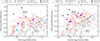 |
Fig. 4. M1 and M2 diagnostic diagrams, firstly presented and discussed in Mazzolari et al. (2024). The colors follow the same scheme as in Fig. 2. |
We note that in the diagnostics presented in Figs. 2, 3, 4 there are some sources lying close enough to the demarcation lines that their line ratios’ error can potentially place them outside from the AGN-only region of the diagrams. We considered all the selected NLAGN whose 1σ uncertainties are compatible with SF-driven photoionization, and we double-checked if they were safely identified as NLAGN in other diagnostics (i.e., without 1σ errors crossing the demarcation line). We identified four NLAGNs with errors compatible with SFG ionization – CEERS-2668, CEERS-3535, CEERS-1836, and CEERS-3585 – and we conservatively decided to mark them only as candidates NLAGNs. CEERS-2900 should also be included in this sample, but given its detection in both the X-ray and radio image of the field it can be safely considered a NLAGN.
3.2. UV diagnostic
In this section, we focus on the diagnostic diagrams involving rest-frame UV lines (Mingozzi et al. 2024; Mascia et al. 2024; Scholtz et al. 2025; Feltre et al. 2016). In particular, we considered the UV diagnostic diagram C3He2-C43 and the diagnostic diagrams involving the so-called high-ionization emission lines, N IV] λ1486, N V λ1243, and [Ne IV] λ2425.
The C3He2-C43 diagnostic diagram reported in Fig. 5 allows us to select one single NLAGN (CEERS-613), whose selection is based on a clear detection of the He II λ1640 line, which places the source well into the AGN-dominated region according to the demarcation lines presented in Hirschmann et al. (2023). The detection of the UV lines involved in this diagram is challenging with only ∼50min of JWST exposure (the average on-source exposure time of the CEERS survey). Also in Scholtz et al. (2025) the number of detections of these lines is low, even if the exposure time per target of the JADES survey was ∼8 times longer than the CEERS observations.
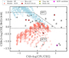 |
Fig. 5. C3He2 versus C43 diagnostic diagrams, selecting only one NLAGN due to the difficulties in detecting rest-UV lines in high-z galaxies with the short exposure times of the CEERS survey. The stacking line ratios and the average errors are not reported because of the poor statistics. The colors follow the same scheme as in Fig. 2. The demarcation lines are those defined in Hirschmann et al. (2023). |
The high-ionization emission lines are characterized by high-photoionization energies that are more likely to be produced in AGNs, due to their harder ionizing radiation, and therefore can be used as indicators of the presence of an AGN, even if hidden. In the diagnostics diagrams involving these lines, we base the identification of NLAGN on the position of the sources compared to the distribution of AGN and SFG photoionization models of Gutkin et al. (2016) and Feltre et al. (2016). In the top panel of Fig. 6 we show the diagnostic diagram involving the N IV] λ1486 emission line, which has an ionization potential of 47eV. This diagnostic allows us to select two NLAGN (CEERS-496, CEERS-1019), based on their extreme position with respect to the distribution of both SFG and AGN photoionization models. However, given the unclear detection of the He II λ1640 line in both these sources, and given the uncertainties in the extension of the SFG region in the diagnostic, we decided to mark these NLAGNs only as candidates. In particular, the source in the upper part of the diagram is CEERS-1019, whose AGN nature has already been discussed in multiple works in the literature, some supporting the presence of an AGN based on a low-significance broad Hβ detection (Mascia et al. 2024; Larson et al. 2023) and some discarding it (Tang et al. 2023) and attributing its spectral properties to exotic SF. In the middle panel of the same figure is represented the diagnostic diagram involving the N V λ1240 emission line (ionization potential of 77eV). In this case, we could select only one source with a N V λ1240 detection, CEERS-23, which we again marked as a candidate due to the undetection of the He II λ1640 line. In the last panel of Fig. 6, we show the [Ne IV] 2424 emission line diagnostic, whose ionization potential is 63eV. We detect the [Ne IV] 2424 line in three different sources (CEERS-1029, CEERS-13061, CEERS-4210), and all of them occupy a region of the diagram covered only by the AGN models, even considering the upper limits in He II λ1640. In this diagnostic diagram (where the [Ne IV] and [Ne III ]lines are ∼ 1000 Å apart one from the other) the dust correction would move the points toward the right, to even more AGN-extreme values.
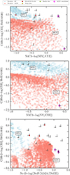 |
Fig. 6. From top to the bottom: C3He2 versus N4C3, C3He2 versus N5C3, C3He2 versus Ne4C3 diagnostic diagrams. The stacking line rations and the average errors are not reported because of the poor statistics. The colors follow the same scheme as in Fig. 2. |
Furthermore, we detect the [Ne V] 3426 emission line (97eV of ionization potential) in one source (CEERS-8299, at z = 2.15) that we marked as AGN given the extremely high-ionization energy required to produce this line. Even if at high-z it has been proposed that the [Ne V] 3426 could also be associated with SF processes (Cleri et al. 2023), it was always related to AGN activity at z < 3 (Mignoli et al. 2013; Barchiesi et al. 2024). Overall, we selected 52 NLAGNs among the initial 217 sources.
3.3. Stack of the AGN and non-AGN samples
In each of the diagnostic diagrams reported in Sect. 3, we also report the line ratios of the stacked spectra of all the selected NLAGN and of the non-AGN selected sources, derived as presented in Sect. 2.3 and shown in Fig. 1. The two stacked spectra were then fit to measure emission line fluxes using Qubspec, following the same procedure as for all the other single spectra and described in Sect. 2.2.
As it is possible to see from the R3N2 diagram, the position of the stacked NLAGN and the non-AGN sources are very close together, with AGN having a slightly larger R3 line ratio. This clearly shows how the BPT diagram and its traditional demarcation lines are no longer useful in effectively separating the AGN population from SFG, probably even for relatively low redshifts (z > 2). We further discuss this point in Sect. 4.1. On the contrary, in the R3S2 diagnostic diagram, the line ratios of the stacked NLAGN spectrum clearly lie in the AGN region of the diagnostic, while the non-AGN one is in the SFG-dominated region. The R3S2 line ratios seem to be still informative for the AGN selection also at (relatively) high-z, as we discuss in Sect. 4.1. The same applies to the R3O1 diagnostic diagram. As for the He2N2 diagram, we note that while the NLAGN stacked spectrum shows a clear detection of the He II 4686 line, which places the final NLAGN stack clearly in the AGN region of the diagnostic, for the non-AGN sample the He II λ4686 line is not detected and the line ratios fall in the SFG region, as expected. This is also a strong point in favor of the goodness of our NLAGN selection since the He II λ4686 line was detected with high-enough S/N only in 5/52 of the NLAGN, 4 of them at z < 3. The fact that this line is clearly detected in the NLAGN spectral stack and that the stack line ratios fall in the AGN region of the diagnostic means that signatures of AGN emission are widely present among our NLAGN sample.
In both the diagnostic diagrams involving the [O III] λ4363 auroral line, NLAGN are characterized by a larger (∼0.3 dex) [O III] λ4363/Hγ line ratio compared to the non-AGN, while the two have a similar O3O2 or Ne3O2 line ratios, meaning that the NLAGN selection is mainly driven by a stronger [O III] λ4363 auroral line in AGN, as discussed in Mazzolari et al. (2024).
We did not put the results of the stack in the rest-UV diagnostic diagrams. This is because the He II λ1640 and C IV lines are available only for 33/155 non-AGN and 7/52 NLAGN, and both these lines are not significantly detected in none of the two stacked spectra. This is expected given the faintness of these lines, the possible stronger effect of obscuration at rest-UV wavelengths, and the observing time of the CEERS survey. The same goes for the high-ionization emission line diagnostics: none of the high-ionization emission lines involved in the diagnostics in Fig. 6 is clearly detected in our stack.
4. Discussion
The IDs and the main physical properties (that will be presented and discussed in the next Sections) of all the 52 NLAGN selected in Sect. 3 are reported in Table C.1.
4.1. Comparison of AGN selection methods
In this section, we discuss the effectiveness of the different diagnostic diagrams reported in Sect. 3. For the discussion below, the term effectiveness refers to the ability of a diagnostic diagram to efficiently select (i.e., isolate in the diagram) NLAGN among all the considered sources.
As presented in the top panel of Fig. 7, most of the NLAGN are selected based on only one single diagnostic diagram (35/52, the 65%), 13 are selected in two different AGN diagnostics, while 4 are selected based on more than two diagnostics diagrams. The approach chosen for the NLAGN selection in this work clearly favors the high-completeness instead of the high-purity criterium, selecting as NLAGN all the sources showing the dominance of the AGN photoionization in at least one diagnostic diagram. However, the fact that most of the NLAGN are selected based on one single NLAGN diagnostic is not surprising. The NLAGN diagnostic diagrams used in our work involve emission lines that cover a wide wavelength range (from rest-UV to rest-optical), over which the spectral features of sources at 1 ≲ z ≲ 9 can vary a lot depending on many parameters (metallicities, stellar population in the host galaxy, radio or X-ray emission, etc.). Given this, different NLAGN diagnostic diagrams are intrinsically sensitive to different AGN properties and, in turn, can become ineffective (and therefore less useful in separating AGNs from SFGs) under different conditions. Additionally, given the wide redshift range of the sources analyzed in this work, not all of them have in their observed spectra all the lines used for the diagnostic reported in Sects. 3.1, 3.2, mostly because lines might be redshift out from the observed wavelength range or fall into a spectral gap.
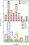 |
Fig. 7. Summarizing plots of the NLAGN selection. Upper: NLAGN counts in the different redshift bins, color-coded by the number of diagnostics in which each NLAGN has been selected. Lower: Distribution of the NLAGN according to the different diagnostic diagrams presented in Sect. 3, as labeled. |
Looking at the lower panel of Fig. 7, we see the distribution of the sources selected by the different diagnostic diagrams with respect to their redshift. The diagnostic diagram that selected the larger number of the AGN is the R3S2, in particular at z < 3, but with a non-negligible number of NLAGN also selected at z ∼ 5. The effectiveness of the R3S2 (but also of the R3O1) diagnostic diagram in the low-metallicity (more frequent at high-z) regime was already pointed out in some recent works investigating the effectiveness of traditional NLAGN diagnostic diagrams to select AGN among low-metallicity dwarf galaxies (Polimera et al. 2022). In particular, they show that the S2 and the O1 line ratios are less metallicity-sensitive and more successful in identifying AGN in these dwarf environments (more similar to those at high-z) than the R3N2 diagnostic. The lower effectiveness of the R3N2 at low metallicities (hence at high redshift) can be a consequence of the nitrogen production channel (Henry et al. 2000) that can determine nitrogen abundance to scale about quadratically with metallicity (at Z > 0.1 Z⊙), hence the [NII]/Hα ratio drops strongly. On the contrary, Sulfur and oxygen aboundances, being directly produced by massive stars through α-processes, can be less dependent on metallicity (Dopita et al. 2013). We also notice that [N II] and [S II] get redshifted out from the reddest grating of the spectra at z ∼ 6.7, while the [O I] gets redshifted out at z ∼ 7.
We further note that [O I] emission can sometimes be excited also by shocks, producing high [O I] /Hα ratios not necessarily driven by a dominant AGN ionization. However, shocks in SFG are generally sub-dominant, as evidenced by the distribution of SDSS galaxies in the BPT and by works selecting this kind of population among SDSS SFG [e.g.][found that shock-dominated SFG are < 1% of the SDSS DR7 SFG]Alatalo16. For this reason, it would be unlikely that such a large fraction of SFG at higher redshift would exhibit shock-driven emission. Shocks can also be an important source of ionizing power in mergers (Medling et al. 2015) and, of course, in AGN (Best et al. 2000). While, after a visual inspection, we did not find strong evidence of ongoing mergers in the majority of the sources selected as NLAGN by the R3O1 diagnostic, we note that 8 out of the 12 NLAGN selected using the R3O1 line ratios are also selected as NLAGN in other diagnostic diagrams, supporting the scenario in which for most of the sources the [O I] line should be driven by AGN photoionization.
In general, at z < 3 the most effective AGN diagnostic diagrams are the R3S2, N2He2, and R3N2, while the large majority of the AGN at z > 3 are selected based on the auroral line diagnostics (both M1 and M2), or based on the detection of high-ionization emission lines. This supports the fact that traditional AGN diagnostic diagrams (in particular the R3N2) become less effective at high-z, mainly due to metallicity-related effects, while diagnostic based on high-ionization emission lines or on the [O III] λ4363 line proved to be effective in selecting AGN also in the early Universe, as already pointed out by Maiolino et al. (2024b), Übler et al. (2023) and Scholtz et al. (2025).
The spectra of the NLAGN selected at z > 6 (together with the main spectral features that lead to the NLAGN classification) are presented in Appendix D.
4.2. Selection of X-ray and radio sources in the diagnostics
In this section, we want to summarize the results related to the X-rays and radio sources involved in our analysis. Among the seven X-ray sources with a spectrum in the CEERS MR sample, two sources (CEERS-3050 and CEERS-3061) are at z < 0.5, and their rest-frame optical and UV lines are not available in JWST spectra. These sources were classified as SFG by the X-ray spectral analysis performed in Buchner et al. (2015). Among the other five X-ray sources, four are selected as NLAGN in at least one of the diagnostics. In particular, the one at highest redshift (CEERS-2808, z = 3.384) is selected as NLAGN only in the R3S2 diagnostic diagram and not in the R3N2 (considering the more conservative demarcation line reported in Scholtz et al. 2025). The only three X-ray sources selected as NLAGN in the BPT diagram are CEERS-2919, CEERS-2904, and CEERS-2900, all at z ≲ 2, the first two also showing a broad Hα emission line (see Appendix A). The only X-ray source not selected in any of the diagnostics is CEERS-2989, at z = 1.433, whose spectrum shows only Hα and [N II] detections and we could not define the R3 line ratio to place it in the above-mentioned diagnostics. It is worth noting that the lack of [O III] λ5007 and Hβ detections in this source is probably due to high obscuration levels. Considering the analysis in Sect. 4.6, we found a lower limit to the ISM obscuration corresponding to AV ∼ 6 mag. The large AGN obscuration of this source is further supported by the CTK obscuration level derived by the X-ray analysis performed in Buchner et al. (2015). However, this source shows a faint broad Hα component, as reported in Fig. A.1.
The two radio-detected sources are CEERS-2900 (that is also X-ray detected) and CEERS-3129, both selected in the R3N2 diagram as well as in the R3S2 one. They also both show strong [N II] emission, in particular CEERS-3129, which could be indicative of a shock (Allen et al. 2008; Nesvadba et al. 2017). Furthermore, CEERS-3129 shows a significant broad Hα component, but no indication of X-ray emission, as we further explore in Sect. 4.9.
4.3. Comparison with previous CEERS AGN selections
Calabrò et al. (2023) attempted to select AGN among the CEERS sources with a MR spectrum using near-infrared emission line diagnostics. To do so, they restricted the redshift range of the sources to 1 < z < 3, therefore considering only 65 sources. Using the R3N2 and R3S2 diagnostic diagrams, the authors selected 8 NLAGN that were classified as NLAGNs also based on at least one NIR diagnostic: CEERS-2919, CEERS-3129, CEERS-2904, CEERS-2754, CEERS-5106, CEERS-12286, CEERS-16406, and CEERS-17496. The first three were marked as BLAGN, as we also found in Appendix A.1. Five of the sources selected as NLAGN by Calabrò et al. (2023) are also selected in our work, while the other three sources were not selected because of the more conservative demarcation lines used in the R3S2 and R3N2 diagnostics or because the [S II] line was not considered detected with enough significance by our fit. The authors also selected five NLAGNs using near-infrared diagnostic diagrams that were classified as SFG based on the optical diagnostic diagrams: CEERS-2900, CEERS-8515, CEERS-8588, CEERS-8710, and CEERS-9413. Among these, the only one that is classified as NLAGN also in our selection is CEERS-2900; the other three were selected as SFG also by our optical diagnostics (even if CEERS-8588 shows a tentative [Ne V] line emission, but we conservatively decided to mark it as a non-detection).
In Davis et al. (2024) the authors investigate the presence of extreme emission-line galaxies (EELG) at 4 < z < 9 using JWST NIRCam photometry in the CEERS program. They used a method to photometrically identify EELGs with Hβ + [O III] or Hα emission of observed-frame equivalent width > 5000 Å. Among the photometrically selected EELGs there are 39 sources with a NIRSpec PRISM or MR spectrum, 25 with a match in our MR parent sample. Among these, 6 are selected as NLAGNs in our work, in other words ∼25%, supporting the non-negligible AGN contamination in the photometric selection of this kind of source, as has already been shown by other works (Amorín et al. 2015).
4.4. AGN prevalence
In Fig. 8, we show the fraction of the selected NLAGN among the CEERS MR sample. In particular, we consider as parent sample all the galaxies with a MR spectrum and with a secure redshift (217 sources). Then we divided the distribution into four redshift bins of Δz = 2 between z = 0 and z = 9, and for each bin, we computed the fraction of AGN compared to the parent sample. The number of sources in the different redshift bins is 122, 85, 59, and 49, going from the lower to the higher redshift bin. We derived an almost constant fraction of AGN among the CEERS MR sources ∼20%. This fraction does not necessarily represent the intrinsic AGN fraction at these redshifts, given the fact that the original selection function of the CEERS spectroscopic survey (necessary to correctly account for completeness corrections) is extremely hard to derive. However, this result agrees well with what was found for the NLAGN selection in the JADES survey by Scholtz et al. (2025). Given the different sensitivities reached by the CEERS and JADES surveys, one would probably expect a lower fraction of NLAGN selected in the CEERS sample since, in most cases, the AGN selection is based on the detection of faint emission lines. At the same time, as we are going to show in Sect. 4.7, the median bolometric luminosity of the NLAGN in the CEERS sample is ∼1 dex higher compared to those selected in JADES, and so the fact that the targets are brighter partially compensate for the shorter exposure times.
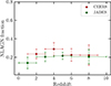 |
Fig. 8. Fraction of the spectroscopically selected NLAGN with respect to the parent sample in this work (CEERS, in red) and in the JADES survey (green) (program ID 1210&3215, Scholtz et al. 2025) in different redshift bins. The errors account for the statistical uncertainties and are computed considering a Poissonian noise. |
4.5. Velocity dispersion
In Fig. 9, we show the distribution of the intrinsic narrow line FWHM of the [O III] λ5007 emission line compared to the redshift of the sources. In particular, we considered only sources with the [O III] λ5007 line detected at S/N > 5. To estimate the intrinsic FWHM, the observed FWHM retrieved by the fit was deconvolved by subtracting in quadrature the instrumental resolution of the grating at the observed wavelength of the [O III] λ5007 line. The instrumental velocity resolution was derived from the [point_source_lsf_f290lp_g395m_QD1_i185_j85.csv] line spread function file, which was calculated from the instrument model (Ferruit et al. 2022), assuming a point-source geometry and a target located in the first MSA quadrant, at the center of shutter (i,j) = (185,85); this procedure is described in de Graaff et al. (2024). The median value of the instrumental resolution is ∼160 km/s.
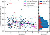 |
Fig. 9. Redshift distribution of the intrinsic [O III] λ5007 line FWHM, resulting from the line-fitting procedure and subtracting the instrumental FWHM. On the left, we also report the median values of the FWHM of NLAGN (magenta), non-AGN (cyan) and of the global population (black) in five different redshift bins. Errors are derived using a bootstrap procedure. There is no significant trend of the FWHM of the sources with redshift. On the right, we report the histogram of the NL-FWHM distribution for AGN (red) and non-AGN (blue). |
The lower and upper boundaries of the observed FWHM distribution are limited by the prior on the width of the line given to Qubespec; that is, 200 km/s < FWHM < 700 km/s. None of the sources, after the subtraction of the instrumental resolution, shows a negative FWHM, but there is a non-negligible number of sources with an FWHM < 200 km/s, meaning that in these cases we are really detecting emission lines at the limits of JWST resolution. Indeed, the cut in S/N and a careful visual inspection confirm beyond any doubt that these lines are real, and, actually, such narrow FWHMs are expected given the trend of decreasing host galaxy stellar mass with redshift and given the fact that with JWST high-resolution spectroscopy were recovered FWHM up to ∼100 km/s (Maiolino et al. 2024b). On the other hand, there are six sources with an intrinsic FWHM > 400 km/s. Four out of these six were classified as AGN using the diagnostic diagrams discussed above; in particular, three of these NLAGN are also low-redshift BLAGN reported in Fig. A.1. Among the analyzed spectra, we did not find any significant residual from the fit of the narrow [O III] λ5007 line that could be indicative of the presence of an outflow component.
In Fig. 9, we also report the median values of the FWHM of the NLAGN population and of the non-AGN in five equally spaced redshift bins. The distribution of AGN and non-AGN, considering the errors, do not differ significantly in any of the redshift bins. We also perform the Kolmogorov-Smirnov (KS) test on the global marginal distributions in FWHM of the two populations (histogram on the right panel), finding a p-value = 0.62, which does not point toward different parent samples of the two distributions. This indicates that the NLAGN we spectroscopically selected among JWST spectra did not significantly impact their host-galaxy ISM, contrary to what was found in other studies on NLAGN samples, where, however, the NLAGN were selected based on other AGN activity tracers. For example, in the X-ray selected AGN sample of the KASHz survey, investigating sources at Cosmic Noon, Harrison et al. (2016) found that ∼50% of the targets have ionized gas velocities indicative of gas dominated by outflows and/or highly turbulent material, with [O III] λ5007 FWHM ≥ 600 km/s. We further discuss the AGN impact on the sources studied in this work in the next sections.
4.6. Obscuration
In Fig. 10, we show the distribution of the AV values obtained from the Balmer line decrement. In particular, to derive the AV we considered the SMC attenuation law (Gordon et al. 2003)5 (RV = 2.74) for sources at z > 3 and the Calzetti et al. (2000) attenuation law for sources at z < 3 (with RV = 3.1). While the Calzetti et al. (2000) attenuation law has been extensively used in the low-z Universe to account for the effects of dust, the choice of the SMC attenuation law is more appropriate for the high-z Universe (Reddy et al. 2015; Shapley et al. 2023), where galaxies are smaller and more compact than in the local Universe (Ono et al. 2023). In particular, we select only those sources that have both Hα and Hβ detected. We assumed CASE B recombination; that is, an intrinsic Hα /Hβ ratio of 2.866. We also considered sources with upper limits in Hβ to derive lower limitsin AV.
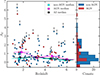 |
Fig. 10. Redshift distribution of the values of AV inferred from the Balmer decrement in sources with detected Hα and Hβ lines. For sources with upper limits on Hβ we derived lower limits on AV. On the left, we also report the median values of AV for NLAGN (magenta), non-AGN (cyan) and for the global population (black) in four different redshift bins. Errors are derived using the bootstrap procedure. On the right, we report the histogram of the AV distribution for AGN (red) and non-AGN (blue). |
We note that a small number of galaxies in Fig. 10 scatter to either surprisingly high values of AV or else negative values, meaning an Hα /Hβ line ratio lower than the dust-free minimum value of 2.86. Sources with a dust-free Hα /Hβ line ratio lower than CASE-B recombination have also been reported recently in the literature (Scarlata et al. 2024; Yanagisawa et al. 2024; McClymont et al. 2024), but in our case these sources all have Hα /Hβ line ratios compatible at 1–2σ with 2.86. However, there is also the possibility that a small number of these outliers is due to small systematics in the NIRSpec grating-to-grating flux calibration; that is, when Hβ and Hα are measured in different gratings. A similar result was indeed also observed in Shapley et al. (2023) on the same sample analyzed here. Even if present, these calibration issues do not affect our NLAGN selection, because the line ratios of the diagnostics presented above involve lines close to each other, and so generally in the samegrating.
In Fig. 10, we also plot the median value of the obscuration considering four different redshift bins and taking separately the two populations of NLAGN and sources not identified as AGN. We did not consider for the median values the upper limits in AV. We did not find a significant evolution of AV with redshift. We also note that the AGN population is characterized, in the lower redshift bin (1 < z < 2.5), by a ∼0.7 mag higher obscuration. At z < 2.5 the average NLAGN obscuration is 1.15 mag compared to the 0.5 mag of non-AGN. On the contrary, when the whole NLAGN and non-AGN populations are taken into account, the average value of the obscuration across all redshifts is very similar, around 0.3 − 0.5 mag.
4.7. Bolometric luminosities
In this section, we investigate the bolometric luminosities of the NLAGN selected in this work. The way to compute the AGN bolometric luminosity is not unique, and it can be done starting from the X-ray luminosity, the luminosity of the BL emission or the UV continuum emission determined by the accretion disk. However, in our case, the majority of the sources are not X-ray detected, they do not have a BL emission, and their continuum is generally undetected. Therefore to estimate the bolometric luminosities, we rely on the dust-corrected narrow line fluxes of the Hβ line, using the calibrations reported in Netzer (2009). These fiducial Lbol for the sample of NLAGN (with available Hβ line) are reported with red squares in Fig. 11. In the same figure, we also report, with a fainter marker, the value of Lbol estimated from the same line fluxes but with the calibration used in Scholtz et al. (2025) and taken from Hirschmann et al. (in prep). In this second case, the bolometric luminosity depends quadratically on the luminosity of the Hβ line, while the Netzer (2009) calibration is linear, determining a difference in the estimated Lbol that can go up to ∼1 dex (on average the bolometric luminosities computed using Hirschmann et al. calibrations are 0.8 dex lower). To verify the reliability of our fiducial values of Lbol we also considered the bolometric luminosity calibrations derived in Lamastra et al. (2009) where the NLAGN bolometric luminosities are derived from the dust corrected [O III] λ5007 line. The Lbol computed using the calibration in Netzer (2009) and those computed using the calibrations in Lamastra et al. (2009) agree well, with a median discrepancy of only ∼0.25 dex.
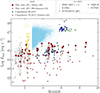 |
Fig. 11. Bolometric luminosities versus redshift of the sample of NLAGN selected in this work (red squares) compared to the bolometric luminosities of other AGN samples selected using JWST spectroscopic observations or pre-JWST, as labeled. The darker red squares represent the baseline bolometric luminosities, derived using Netzer (2009) calibration, while the fainter red squares show the values of the bolometric luminosities obtained using the same calibration adopted in Scholtz et al. (2025). The compilation of JWST selected BLAGN includes the sources taken from Maiolino et al. (2024b), Harikane et al. (2023), Matthee et al. (2024), Übler et al. (2023), Kocevski et al. (2023). SDSS BLAGN at z > 3 (light blue crosses) are taken from Wu & Shen (2022). AGN from the KASHz and SUPER surveys at Cosmic Noon (gray and red gold crosses) are taken from Harrison et al. (2016) and Kakkad et al. (2020), respectively. QSOs samples at Epoch of Reionization are taken from Zappacosta et al. (2023) (green crosses, HYPERION sample), and Mazzucchelli et al. (2023) (dark-blue crosses, XQR-30). |
However, It is worth noting that all these calibrations assume that the lines used to derive Lbol are dominated by the AGN emission. This assumption is not necessarily true for the whole sample of NLAGN, and therefore, our Lbol should be generally taken as upper limits. For BLAGN at z ≤ 2 presented in Fig. A.1, we computed the bolometric luminosities considering the same relation used in Harikane et al. (2023) to determine the bolometric luminosities of the BLAGN at z > 4.5 of this sample, i.e the bolometric luminosity calibration derived in Greene & Ho (2005) from the (dust corrected) broad Hα emission.
In Fig. 11, we compare the distribution of Lbol of our sample with the AGN bolometric luminosities of other samples at comparable redshifts and taken from the literature. In particular, we report AGN bolometric luminosities derived both from JWST spectroscopic studies and from pre-JWST surveys. Given the bolometric luminosities of z > 3 AGN detected before the advent of JWST, it is clear that we are now able to sample a completely new regime in the luminosity-redshift space. Comparing the bolometric luminosities of our sample with those of the NLAGN selected sample from Scholtz et al. (2025), we note that our targets are on average ∼1.5 dex more luminous considering our fiducial calibration, but still more luminous even considering the luminosities derived with the calibration of Hirshman et al. (in prep). On the opposite, the AGN luminosities of our sample are comparable, in the same redshift range, with the distribution of Lbol derived from multiple samples of BLAGN detected with JWST.
4.8. Host galaxies’ properties
In Fig. 12, we show the results from the SED-fitting performed on the whole sample of 217 sources that is described in Sect. 2.4. In particular, we compare the trend with redshift of the ratio between the SFR derived from the CIGALE SED fitting and the one obtained from the main sequence (MS) reported in Popesso et al. (2023) at the stellar mass (M*, obtained from the fit) and redshift of each source. We note that sources at z < 4 are generally distributed almost symmetrically with respect to the MS, with the median value of log SFR/SFRMS ∼ 0.1. On the contrary, at z > 4, sources appear to be systematically above the corresponding MS, with a median value of log SFR/SFRMS ∼ 0.4, in other words with SFRs 2-3 times larger than the respective MS SFR. Sources with larger SFRs are also the sources with the lower M*, some of them reaching log M* ≲ 8. This means that the high-z galaxies analyzed in this sample seem to have, on average, a higher MS normalization, being less massive and more star-forming than expected from the MS. Different works, taking advantage of JWST spectroscopy, have already shown that high-z galaxies are frequently in a state of intense or bursty SF (Dressler et al. 2023; Looser et al. 2025; Endsley et al. 2024), probably driven by a higher SF efficiency related to the lower metallicities of high-z galaxies. However, this apparent above-MS behavior at high-z could also be due to a selection effect. Indeed, given that we are investigating a spectroscopic sample, we are probably more biased toward high SFR, in particular at high-z.
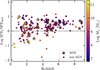 |
Fig. 12. Redshift distribution of the ratio between the SFR derived from the SED-fitting and the SFR computed from the MS relation derived by Popesso et al. (2023) at the redshift and M* of each source. We plot AGN and non-AGN sources with stars and circles, respectively. The sources are color-coded based on the stellar mass, as derived from the SED-fitting. |
For sources not selected as AGN, we also compared the SFR inferred from CIGALE to the values obtained from the Hα line (using the measured dust-corrected Hα luminosity and the relations reported in Shapley et al. 2023). On average, we find a good agreement, with log SFRHα = 0.7 log SFRSED − 0.1 with 0.25 dex of scatter.
The AGN distribution in Fig. 12 is in agreement with the distribution of the other sources not selected as AGN: considering the median distribution of the ratios of the two SFRs, even in different redshift bin, AGN and SFG are indistinguishable, as already found by other works (Ramasawmy et al. 2019). The AGN quenching effect on the host galaxy SF is still a largely debated topic (Bugiani et al. 2025; Man & Belli 2018; Beckmann et al. 2017; Scholtz et al. 2018), and in this case, we do not note a negative impact of the AGN feedback on SF in the host galaxy. This finding is also in line with recent studies based on various cosmological simulations, according to which star formation quenching is not primarily driven by the instantaneous AGN activity but the integrated black hole accretion (as traced by black hole mass Piotrowska et al. 2022; Bluck et al. 2023; Scholtz et al. 2024b). The AGN contribution to the final SED is measured in CIGALE by the parameter fAGN, which corresponds to the fraction of the AGN luminosity with respect to the galaxy one in the rest-frame 0.1–2 μm. As expected, given the NLAGN nature of our sources, for most of the NLAGN, the fit returned a fAGN < 0.5 according to the scenario, already discussed in Sect. 4.5 and Sect. 4.6, that the AGN activity of the selected NLAGN is significantly buried by the host galaxy, in particular in the rest-frame optical part of the SED traced by the available photometry. This scenario, and the absence of asignificant impact of the AGN activity over the host galaxy properties, is even more supported by the fact that we did not find relevant signatures of outflows in our spectroscopic analysis, in particular in the high-z galaxies.
From the NLAGN SED-fitting, we also derived the AGN bolometric luminosities (sum of the disk emission plus the one reprocessed by the tours). However, due to the limited photometric range (the reddest filter is F770W for sources with JWST photometry and IRAC4 for sources with 3D-HST photometry), in most of the cases, we were not able to explore the rest-frame MIR NLAGN emission and the AGN bolometric luminosity is usually largely unconstrained. By selecting only those sources with a reliable bolometric luminosity from the SED-fitting, and comparing these values with the Lbol estimated in Sect. 4.7, we found that the median distributions agree well: the median value of the bolometric luminosity from the Hβ line is ∼0.23dex larger than the one derived from the SED-fitting, but the scatter goes up to ∼1 dex.
4.9. X-ray weakness
As is described in Sect. 2.5, we performed a detailed analysis of the X-ray and radio counterparts of the selected NLAGN. Four out of five of the X-ray sources classified as AGNs by the X-ray analysis in Buchner et al. (2015) are also classified as AGNs by our NLAGN diagnostics. All the other 48 NLAGN do not show any X-ray counterpart. Therefore, we decided to perform an X-ray stacking analysis on our sample, using CSTACK as is described in Sect. 2.5. In particular, we decided to divide the sample of NLAGN in two redshift bins, equally populated, using z = 4.5 as the dividing threshold. We also include in our analysis the BLAGN selected at z > 4.5 in CEERS by Harikane et al. (2023), since none of them show any indication of X-ray emission and to perform a more complete analysis on the AGNsample among the CEERS MR spectra. We did not stack the sample of low-z BLAGNs presented in Appendix A because 3 out of 4 of these sources are X-ray detected (except CEERS-3129, which will be discussed later). The median redshifts of the three AGN samples are 2.37 for the low-redshift NLAGNs, 5.50 for the high-z NLAGNs, and 5.43 for the high-z BLAGN sample. In Fig. 13, we show the stacking maps in the SB and HB for the two NLAGN redshift bins and for the BLAGNs, respectively. Given the median redshift of the samples, and considering the SB as the reference observing band since it provides the deepest constraint, we are investigating, on average, the following rest-frame X-ray energy bands: ∼1.7–6.5 keV for the low-z NLAGN sample and ∼3.5 − 13keV for the other two samples. The stacking analysis did not reveal any X-ray detection in any of the sub-samples. This is quite surprising given the rest-frame energy range tested and the depth of the X-ray observations. To check whether the non-detections in the stacking of the NLAGN were due to possible galaxy contamination in the NLAGN sample, we also performed the same stacking but considering only NLAGN selected in more than two diagnostics diagrams, but again, the X-ray analysis did not reveal any detection. Therefore, we wanted to test if such X-ray non-detections would be compatible or not with the expected X-ray luminosities of these objects.
 |
Fig. 13. 30″×30″cutouts of the X-ray stacking image in the observed SB (0.5–2 keV) and HB (2–8 keV) of the three samples taken into account. From top to bottom: BLAGNs, NLAGNs at z > 4.5, and NLAGNs at z < 4.5. None of the samples show a detection in either band. |
We used the Lbol − L2−10 keV luminosity relations derived by Duras et al. (2020) to compute the expected X-ray luminosities given the baseline dust-corrected bolometric luminosities computed in Sect. 4.7 for our sample of NLAGN. For the BLAGN, instead, we used the bolometric luminosities computed in Harikane et al. (2023) using the Hα broad emission. The comparison between the expected X-ray luminosities and the upper limits derived from the stacking is shown in Fig. 14. For all the AGNs, the upper limits of their observed X-ray luminosities are largely below the expected X-ray luminosities, posing severe constraints on their X-ray production and emission. The X-ray deficit is ∼1.3 dex for BLAGNs and for the sample of NLAGNs at z > 4.5, and is ∼2 dex for the NLAGNs at z < 4.5. The X-ray deficit of this last sample is particularly surprising, given the fact that most of these low-z NLAGNs were selected using the traditional BPTs diagnostic diagrams, which are not expected to fail the NLAGN selection at low-z.
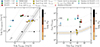 |
Fig. 14. Results coming from the X-ray stacking, showing a significant X-ray weakness of all three samples of NLAGNs at z < 4.5, NLAGNs at z > 4.5, and high-z BLAGNs. Left: Expected X-ray luminosity versus observed X-ray luminosity (in the 2–10 keV band) of the three AGN samples we used for the stacking, as labeled. We also plot the sources in the CEERS MR sample with an X-ray detection color-coded by their obscuration level, as derived from the X-ray spectral analysis (Buchner et al. 2015). Diamonds refer to observed X-ray luminosities, while circles refer to the intrinsic X-ray luminosities derived from the X-ray analysis. Errors bars mark the error on the intrinsic X-ray luminosities of the sources reported in Buchner et al. (2015). The result from the X-ray stacking of these X-ray detected sources is reported as a gold diamond, while the gold circle considers the median of the intrinsic X-ray luminosities of the X-ray sources. The dashed lines correspond to the shift from the observed to intrinsic X-ray luminosities. In cyan, we report the z = 1.037 BLAGN CEERS-3129, presented in Appendix A. Right: Ratio between the mean bolometric luminosity of the three AGN samples (derived using the values computed in Sect. 4.7) and the observed X-ray luminosity upper limits versus the mean bolometric luminosities. The orange line shows the reference L2 − 10 keV − Lbol relation derived by Duras et al. (2020) and used to derive the expected X-ray luminosity of the sources. The empty hexagons represent the lower limits derived from the X-ray stack of the JWST-selected BLAGNs (red) and NLAGNs (green for z > 3 and blue for z < 3) on the CDFS and CDFN (Maiolino et al. 2025). |
We further check that even taking the bolometric luminosities derived using the calibration of Hirschmann et al. (in prep.) (shown as faint red squares in Fig. 11) the results remain almost unchanged, with the median expected X-ray luminosities of the two NLAGN samples decreasing only of ∼0.2 dex.
In Fig. 14, we also show the distribution of the X-ray detected sources in our MR spectroscopic sample together with the position of their X-ray stack. In particular, for each X-ray source, we plot with a diamond the observed X-ray luminosity derived from their X-ray flux assuming Γ = 1.9, namely applying the same procedure as was done for the stack of the other sources. As expected, X-ray sources whose spectral analysis revealed larger column densities are on the left of the 1:1 relation, with a deviation up to ∼1.5 dex for CEER-2989, whose spectral analysis revealed a column density of log (NH/cm−2) ∼ 25. This is because the spectral index, Γ = 1.9, does not properly account for the harder spectrum of these heavily obscured sources. For each X-ray source, we also plot with circles the intrinsic, absorption corrected, X-ray luminosity derived in Buchner et al. (2015), which generally reduces the deviation from the 1:1 relation, especially if we take into account the large uncertainties on the intrinsic X-ray luminosities of the most obscured X-ray AGN. The same applies to the position of the stack of these X-ray sources: when we considered the observed X-ray luminosity (derived from the X-ray stacking) the point slightly deviates from the median expected X-ray luminosity, but if we correct for the absorption the X-ray luminosities (considering the median intrinsic X-ray luminosity on the x axis), then the golden circle perfectly aligns with the median expected X-ray luminosity of these sources.
The same conclusions about the different samples can also be drawn by looking at the right panel in Fig. 14 where we compare the position of the sources with respect to the Lbol − L2−10 keV relation of Duras et al. (2020). In the plot on the right we also show the lower limits derived in Maiolino et al. (2025) from the X-ray stacking analysis performed on JWST selected BLAGN and NLAGN on the Chandra Deep Field South (CDFS, with 7Ms of Chandra observations Liu et al. 2017) and Chandra Deep Field North (CDFN, 2Ms Xue et al. 2016).
In both figures, we also show in cyan the position of the peculiar source CEERS-3129. This is a BLAGN at z = 1.037 (whose broad Hα component is shown in Appendix A), it is not detected in the X-ray image and shows an X-ray deficit of ∼2 dex. This source is also characterized by a consistent dust obscuration: from the Balmer decrement derived in Sect. 4.6 we found AV = 2.12. Since the broad Hβ component is not detected and its upper limit would return an extremely large AV, we assumed for the dust correction of the broad Hα emission (and therefore for the bolometric luminosity) the value of AV derived from the NLR. However, this implies that the bolometric luminosity of CEERS-3129 might be underestimated and, consequently, also its expected X-ray luminosity and the amount of its X-ray weakness. Considering the dust-corrected bolometric luminosity, the lower limit to the X-ray weakness of CEERS-3129 is ∼2 dex.
s Assuming that these sources are really AGNs, the two possible scenarios that can justify such a lack of X-ray emission are:
-
Obscuration coming from large column densities, larger than the CTK limit (log (NH/cm−2) > 24), and/or
-
An intrinsic X-ray weakness due to a possible different accretion disk/corona structure. This can determine, for example, a larger ratio between optical and X-ray fluxes due to a lower efficiency of the corona in producing X-rayphotons.
Yue et al. (2024), analyzing a sample of so-called “little red dots” (LRDs) showing clear AGN signatures (as the detection of a broad Hα component) and selected from various fields covered by JWST imaging and spectroscopy, found a similar result. The amount of X-ray weakness in the LRD is comparable to what we found in this work for the sample of BLAGN at high-z, while they did not investigate the population of NLAGN. In Yue et al. (2024), the authors suggest an intrinsic X-ray weakness as a possible origin of this discrepancy or a wrong AGN classification of these sources; in the latter case, the broad Hα component might be due to fast galactic outflows (with velocities ∼1000km/s). In our case, however, we did not detect any signature of outflows in any of the forbidden lines of the BLAGN. More evidence and strong arguments against the outflow scenario have been presented by Juodžbalis et al. (2024b).
Also Maiolino et al. (2025), considering a large sample of BLAGNs and NLAGNs spectroscopically selected in the JADES survey over the CDFS and CDFN, show that almost all the AGNs discovered by JWST lack any X-ray detection, even in the stack. In this work, the authors investigated different possible origins of this X-ray weakness, focusing in particular on the three possibilities reported above and finding indications in support of one or the other. In particular, they found an enhanced EW(Hαbroad) in these sources, which could suggest that the BLR is distributed with a large covering factor around the central source, acting as a dense dust-free absorbing medium that can potentially reach CTK column densities. On the other hand, the authors also find that many of the AGNs newly discovered by JWST have features in common with the population of narrow-line Seyfert 1 (NLS1), which are known to have a steep X-ray spectrum (with Γ > 2 − 3, and therefore more shifted toward a softer X-ray emission) and/or are characterized by high accretion rates, which are expected to result in a weaker X-ray emission, especially at high redshift, where higher rest frame energies are probed in the Chandra bands.
4.10. Radio stacking to discriminate the nature of X-ray weakness
To discriminate between the heavily obscured versus intrinsic X-ray weakness scenario and explain the observed X-ray weakness of these AGNs, we took into account the 1.4GHz radio image of the EGS field (Ivison et al. 2007). Different works have shown that the physical processes and the magnetic fields at the origin of the hot corona, where the inverse Compton scattering produces the AGN X-ray emission, are also responsible for (at least part of) the synchrotron radiation at the origin of the AGN-related radio emission (Laor & Behar 2008; Panessa et al. 2019). The connection between these two emissions is also at the basis of the so-called fundamental plane relations (Merloni et al. 2003) or of X-ray – radio luminosity relations reported in different works in the literature (D’Amato et al. 2022; Panessa et al. 2019; Fan & Bai 2016). Radio emission is generally largely unaffected by obscuration and can pass freely even from the most obscured environments, contrary to the X-rays that are almost completely absorbed at CTK hydrogen column densities.
However, some works show that even the radio emission can be partially or completely absorbed by the BLR clouds if their uniform distribution is also dense enough to determine free-free absorption (Juodžbalis et al. 2024b, Mazzolari et al., in prep.). However, it is still not clear whether the X-ray and radio emissions originate and are distributed on the same scale, and, therefore, if the effect of obscuration from BLR clouds can suppress both or not (Paul et al. 2024). For example, in Laor & Behar (2008) the authors found that the smallest possible scale of radio emission (ν ∼ 1 − 5 GHz) in radio-quiet (RQ) AGN, e.g., coming from a compact radio corona or jet base, should originate from a region ≥100 times the extent of the X-ray emitting core. In this case, the radio emission would probably originate (or be being mainly distributed) outside of the BLR without being absorbed. Therefore, in the following, we assume that there is not a free-free absorption effect on the radio emission of the NLAGN and BLAGN investigated in this work, and we leave a more detailed discussion to Mazzolari et al. (in prep.).
Consequently, if these AGNs are normal AGNs (in terms of bolometric to intrinsic X-ray luminosity), and heavily obscured (but without absorbing also the radio emission), we might expect not to detect their X-ray emission, but we would expect to detect their radio emission at the level returned by the intrinsic X-ray to radio luminosity relations derived in the literature. On the contrary, if the radio image is deep enough to detect the expected AGN radio emission, but none is detected, we would prefer a scenario in which both the radio and X-ray emissions are intrinsically lower with respect to what is observed in normal AGN at lower redshifts. None of the NLAGNs or BLAGNs are detected in the 1.4 GHz image of the field, apart from two sources CEERS-2900 and CEERS-3129. Therefore, we performed a detailed stacking analysis at the position of the sources, as is described in Sect. 2.5, considering the same three samples as for the X-ray stacking. The radio stacking analysis did not recover any 1.4GHz detection (see Fig. 15), but allowed us to derive upper limits on the median radio luminosities of the sources in the three samples. We compared these values with the expected AGN radio luminosities. Given the expected (and intrinsic) X-ray luminosities of the sources derived in Sect. 4.9, we can estimate the expected 1.4 GHz luminosities using the L1.4 GHz − L2 − 10 keV luminosity relation derived for radiatively efficient radio-quiet (RQ) AGN by D’Amato et al. (2022). The assumption that the sources are RQ is reasonable given that the fraction of radio-loud (RL) AGN has been found to be ∼10% of the radio AGN population by different works, and it is not observed to vary with redshift (Liu et al. 2021; Williams & Röttgering 2015).
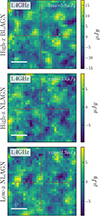 |
Fig. 15. Median radio stacking of the three AGN samples taken into account. From top to bottom, we report 25″×25″cutouts of BLAGNs, NLAGNs at z > 4.5, and NLAGNs at z < 4.5. None of the samples show radio detection. For each stack, we report the noise (rms) value in the top right corner. |
It is worth noting that the effectiveness of this test also depends on the fact that the AGN-related radio emission has to be dominant over the radio emission coming from star formation in the host galaxy. To check this, we considered the SFRs derived for these AGNs from the SED fitting in Sect. 4.8, and we converted them into radio luminosities using the relations reported in Novak et al. (2017), Delvecchio et al. (2021). For all the three AGN samples the median 1.4GHz luminosities due to star formation are ∼1.5 dex lower than the AGN radio luminosity derived from the L1.4 GHz − L2 − 10 keV luminosity relation of D’Amato et al. (2022).
The comparison between the observed and the expected 1.4 GHz luminosities of the three AGN samples is presented in Fig. 16, together with the upper limits of the single sources in the three samples. Unfortunately, the AEGIS20 radio image is too shallow to give conclusive constraints on the nature of the X-ray weakness of these AGN, being the upper limits of the stack compatible with the expected radio luminosities. We also explore the possibility that the bulk of the sources are instead RL, and, therefore, we computed the expected radio luminosities of the three stacks considering the L1.4 GHz − L2 − 10 keV luminosity relation of Fan & Bai (2016), derived for radiatively inefficient RL AGN. In this case, the observed upper limits on the 1.4 GHz luminosities are different orders of magnitudes lower than expected. This excludes that the bulk of our sources is dominated by RL AGN.
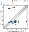 |
Fig. 16. Expected 1.4 GHz radio luminosity versus observed radio luminosity from the stack of the three AGN samples, as labeled. The diamonds refer to the assumption that AGN are RQ, while circles to the hypothesis that sources are RL. We also show the positions of the single sources according to the color of the respective sample. With a cyan diamond, we report the z = 1.037 BLAGN CEERS-3129 (presented in Appendix A). The purple diamond represents the position of CEERS-2900 with the expected L1.4GHz derived using the RQ AGN relation, while the purple circle marks the expected L1.4GHz derived using the RL AGN relation. The shaded gray region represents the dispersion of the L1.4GHz − L2 − 10keV luminosity relation derived for radio-quiet AGN by D’Amato et al. (2022). |
In Fig. 16, we also report the position of the two radio-detected sources, CEERS-2900 and CEERS-3129, at z = 1.9 and z = 1.03, respectively. The first has a 1.4 GHz radio flux of 58 mJy, which corresponds to an observed radio luminosity of L1.4 GHz ∼ 1043 erg/s. If we assume that CEERS-2900 is a RQ AGN, the expected radio luminosity given its intrinsic 2–10 keV X-ray luminosity reported in Buchner et al. (2015) (where the source is classified as a CTK AGN) is only L1.4 GHz,exp = 6 × 1039 erg/s. This strongly points toward the RL nature of this source. Indeed, considering the RL L1.4 GHz − log L2−10 keV luminosity relation reported in Fan & Bai (2016), the observed and expected radio luminosities correspond almost perfectly.
CEERS-3129 has instead a 1.4 GHz radio flux of 286 μJy that translates into a radio luminosity L1.4 GHz ∼ 1040erg/s. The value of the expected L1.4 GHz, computed starting from the expected L2 − 10 keV luminosity, is almost consistent with the hypothesis of CEERS-3129 being a RQ AGN, since the observed and expected radio luminosities are consistent within 2σ. This is even truer if we recall that the expected L2 − 10 keV, derived from Lbol computed using the dust-corrected broad Hα emission, is probably underestimated because the obscuration of the broad Hα component is probably larger than the one derived from the narrow-line Balmer decrement (see Sect. 4.9).
The fact that the expected and observed radio luminosities of CEERS-3129 almost correspond supports the extreme CTK scenario to explain the observed X-ray weakness of this source. However, this scenario is not free from problematics. For example, it requires the CTK envelope around the central SMBH absorbing the X-ray emission to be almost completely dust-free to allow the broad Hα emission to escape. A natural solution to this problem is that the BLR clouds themselves, with large column densities distributed with approximately a 4π covering factor, absorb the X-ray photons, as discussed and analyzed in Maiolino et al. (2025).
5. Conclusions
In this work, we have analyzed the public JWST/NIRSpec MR spectra of the CEERS survey (PID.1340) to identify NLAGNs using multiple emission-line diagnostic diagrams. First, we attributed spectroscopic redshift to 217 out of the 313 targets observed with the JWST/NIRSpec MR setup. We performed spectral line fitting using QubeSpec, and fitting separately different complexes of emission lines, ranging from rest-UV to rest-optical. We considered ten different emission line diagnostic diagrams to perform the NLAGN selection, using both demarcation lines taken from the literature and also exploiting the distribution of SFG and AGN photoionization models taken from Gutkin et al. (2016) and Feltre et al. (2016). This process led to the identification of 52 NLAGNs, whose IDs and main physical parameters are reported in Table C.1 to allow the scientific community to perform further studies. The main results are the following:
-
Traditional AGN diagnostic diagrams, in particular the BPT (R3N2), are less effective in selecting AGNs at z > 3, because high-z galaxies and AGNs generally overlap in these diagnostics due to the different physical conditions of high-z sources. For the high-z regime, the most effective AGN diagnostic diagrams are the ones based on the [O III] λ4363 line (Mazzolari et al. 2024) or on the high-ionization emission lines.
-
We selected ten NLAGNs at z > 6 (four of them marked only as candidate NLAGNs), whose spectra are reported in Appendix D.
-
The NLAGN selection includes only one out of the eight BLAGNs at z > 4.5 selected in Harikane et al. (2023) – CEERS-1244 – four out of five of the X-ray sources with a CEERS MR spectrum and classified as AGNs by the X-ray spectral analysis in Buchner et al. (2015), and both the radio detected sources reported in the radio catalog of Ivison et al. (2007).
-
NLAGN represent ∼20% of the sources analyzed in this work. This fraction is almost constant across different redshifts and agrees well with what was found by Scholtz et al. (2025) for the NLAGN population selected among the spectra of the JADES survey.
-
We analyzed the distributions of [O III] λ5007 narrow-line FWHMs of the AGN and non-AGN samples without finding significant differences in the distributions of the two populations. This suggests that the NLAGNs identified in this work are not significantly impacting the ISM of their host galaxies. This is probably due to the fact that, thanks to the sensitivity of JWST, we are selecting a fainter NLAGN population that is characterized by having a weaker impact on the host galaxy and lacking powerful outflows (contrary to what has been observed for other NLAGN samples at lower redshifts). Furthermore, in many cases, and in particular for low-mass high-redshift sources, the FWHMs are very close to the resolution limit of JWST.
-
We also investigated the average obscuration level of the sources by computing the AV values from the Balmer decrements. We did not find a significant evolution with redshift in the value of AV. We also note that the AGN population is characterized, in the lower-redshift bin 1 < z < 2.5, by a ∼0.7 mag larger obscuration, while in the other redshift bins the median value of obscuration of NLAGNs and non-AGN sources is almost the same.
-
We computed the bolometric luminosities of the sources using the dust-corrected Hβ fluxes and the scaling relation reported in Netzer (2009). The range of Lbol spanned by our NLAGN sample at z > 3 is much lower than the AGN bolometric luminosities reported in any pre-JWST samples, but ∼1 dex larger than bolometric luminosities of the JWST selected NLAGN reported in Scholtz et al. (2025) selected in the JADES survey (where the exposure times are significantly longer). We tested the robustness of the derived bolometric luminosities by comparing our baseline results with the ones derived using the calibrations reported in Lamastra et al. (2009) for the [O III] λ5007 line, finding a good agreement between the two.
-
We performed a SED-fitting analysis using CIGALE to derive the main physical properties of the host galaxies for the sample of NLAGNs and non-AGNs. We found that, on average, sources at z > 4 deviate from the main sequence of Popesso et al. (2023), moving toward higher SFR values than what is predicted by the MS. The range of stellar masses extends down to ∼107M*. We did not find any significant difference in the SFR or M* distribution of the NLAGN compared to the ones of the parent sample, suggesting that any potential positive or negative AGN feedback on the host-galaxy SFR is not significantly taking place. This is in agreement with the lack of significant outflow detections in their spectra.
-
We investigated the X-ray properties of the selected NLAGNs and of the BLAGNs selected in Harikane et al. (2023). We found that none of the BLAGNs is detected in the X-ray image of the field and that only 4 of the 52 NLAGNs are X-ray detected. We performed an X-ray stacking analysis on the AGNs that are not X-ray-detected, finding a significant X-ray deficit between their expected X-ray luminosities (given their bolometric luminosity) and what comes from the X-ray stacking. This observed X-ray weakness is ∼1.3 dex for the high-z BLAGNs and for the sample of NLAGN at z > 4.5, and ∼2 dex for the NLAGN at z < 4.5. We tried to investigate the origin of the X-ray weakness by studying the radio emission of these sources, which can help to disentangle the heavily obscured AGN scenario from the intrinsic X-ray weak one. Unfortunately, the radio observation covering the region of the CEERS survey is not deep enough to provide a conclusive answer. However, this shows the key role that present and future deep radio continuum observations can have in helping us understand the problem of the X-ray weakness of high-z AGNs. Interestingly, one of the low-redshift BLAGNs, CEERS-3129, is undetected in the deep X-ray image (showing an X-ray deficit of ∼2 dex), but it is detected in the radio image of the field, with a radio luminosity compatible with a RQ AGN nature. The radio detection of CEERS-3129 supports the CTK AGN scenario at the origin of the observed X-ray weakness.
JWST is allowing us to reveal the population of heavily obscured AGNs up to very high redshifts (z > 8) and, at the same time, to investigate the NLAGN population at low redshifts with a spectroscopic sensitivity never explored by pre-JWST surveys. This work highlights the necessity of defining new NLAGN diagnostic diagrams and, in general, different and complementary AGN selection techniques suited for the identification of high-redshift AGNs. Future works will have to explore in more detail the actual number density and the demography of these objects in the early Universe, carefully accounting for the selection function of each spectroscopic campaign. We also stress that a multiwavelength approach, such as the one outlined in this work, is necessary to explore and potentially provide answers to the peculiar features characterizing high-redshift AGNs. In this sense, the future Square Kilometer Array Observatory (SKAO) and the Advanced X-Ray Imaging Satellite (AXIS) will be crucial to reveal the actual radio and X-ray properties of these objects.
We used for the attenuation curve a fit to the average SMC-bar Aλ/AV data points reported in Table 4 of Gordon et al. (2003). We found that the Aλ/AV analytic expression reported in their Eqs. (4)–(5) does not correctly fit their observed data points at λ > 3030 Å and has A(λ = 5500 Å)/AV ≠ 1.
Te = 104, ne = 100 cm−3 (Osterbrock & Ferland 2006).
Acknowledgments
GM acknowledges useful conversations with Andrea Comastri, Roberto Decarli, Sandro Tacchella, William Baker, Callum Witten, Lola Danhaive, Ignas Juodzbalis, Amanda Stoffer, Brian Xing Jiang, and William McClaymont. FDE, JS, RM, and XJ acknowledge support by the Science and Technology Facilities Council (STFC), from the ERC Advanced Grant 695671 “QUENCH”, and by the UKRI Frontier Research grant RISEandFALL. RM also acknowledges funding from a research professorship from the Royal Society. HÜ gratefully acknowledges support by the Isaac Newton Trust and by the Kavli Foundation through a Newton-Kavli Junior Fellowship. IEL acknowledges support from the Cassini Fellowship program at INAF-OAS and the European Union’s Horizon 2020 research and innovation program under Marie Sklodowska-Curie grant agreement No. 860744 “Big Data Applications for Black Hole Evolution Studies” (BiD4BESt).
References
- Abazajian, K. N., Adelman-McCarthy, J. K., Agüeros, M. A., et al. 2009, ApJS, 182, 543 [Google Scholar]
- Aird, J., Coil, A. L., Georgakakis, A., et al. 2015, MNRAS, 451, 1892 [Google Scholar]
- Alatalo, K., Cales, S. L., Rich, J. A., et al. 2016, ApJS, 224, 38 [NASA ADS] [CrossRef] [Google Scholar]
- Allen, M. G., Groves, B. A., Dopita, M. A., Sutherland, R. S., & Kewley, L. J. 2008, ApJS, 178, 20 [Google Scholar]
- Amorín, R., Pérez-Montero, E., Contini, T., et al. 2015, A&A, 578, A105 [NASA ADS] [CrossRef] [EDP Sciences] [Google Scholar]
- Baes, M., Verstappen, J., De Looze, I., et al. 2011, ApJS, 196, 22 [Google Scholar]
- Baldwin, J. A., Phillips, M. M., & Terlevich, R. 1981, PASP, 93, 5 [Google Scholar]
- Barchiesi, L., Vignali, C., Pozzi, F., et al. 2024, A&A, 685, A141 [NASA ADS] [CrossRef] [EDP Sciences] [Google Scholar]
- Beckmann, R. S., Devriendt, J., Slyz, A., et al. 2017, MNRAS, 472, 949 [NASA ADS] [CrossRef] [Google Scholar]
- Best, P. N., Röttgering, H. J. A., & Longair, M. S. 2000, MNRAS, 311, 23 [NASA ADS] [CrossRef] [Google Scholar]
- Bluck, A. F. L., Piotrowska, J. M., & Maiolino, R. 2023, ApJ, 944, 108 [NASA ADS] [CrossRef] [Google Scholar]
- Bogdán, Á., Goulding, A. D., Natarajan, P., et al. 2023, arXiv e-prints [arXiv:2305.15458] [Google Scholar]
- Bongiorno, A., Merloni, A., Brusa, M., et al. 2012, MNRAS, 427, 3103 [Google Scholar]
- Boquien, M., Burgarella, D., Roehlly, Y., et al. 2019, A&A, 622, A103 [NASA ADS] [CrossRef] [EDP Sciences] [Google Scholar]
- Bruzual, G., & Charlot, S. 2003, MNRAS, 344, 1000 [NASA ADS] [CrossRef] [Google Scholar]
- Buchner, J., Georgakakis, A., Nandra, K., et al. 2015, ApJ, 802, 89 [Google Scholar]
- Bugiani, L., Belli, S., Park, M., et al. 2025, ApJ, 981, 25 [NASA ADS] [CrossRef] [Google Scholar]
- Bunker, A. J., Saxena, A., Cameron, A. J., et al. 2023, A&A, 677, A88 [NASA ADS] [CrossRef] [EDP Sciences] [Google Scholar]
- Bushouse, H., Eisenhamer, J., Dencheva, N., et al. 2022, https://doi.org/10.5281/zenodo.7429939 [Google Scholar]
- Calabrò, A., Pentericci, L., Feltre, A., et al. 2023, A&A, 679, A80 [NASA ADS] [CrossRef] [EDP Sciences] [Google Scholar]
- Calzetti, D., Armus, L., Bohlin, R. C., et al. 2000, ApJ, 533, 682 [NASA ADS] [CrossRef] [Google Scholar]
- Cameron, A. J., Saxena, A., Bunker, A. J., et al. 2023, A&A, 677, A115 [NASA ADS] [CrossRef] [EDP Sciences] [Google Scholar]
- Camps, P., & Baes, M. 2015, Astron. Comput., 9, 20 [Google Scholar]
- Carniani, S., Hainline, K., D’Eugenio, F., et al. 2024, Nature, 633, 318 [CrossRef] [Google Scholar]
- Casey, C. M. 2012, MNRAS, 425, 3094 [Google Scholar]
- Miyaji, T., Griffiths, R. E., & C-COSMOS Team 2008, AAS/High Energy Astrophys, 10, 4.01 [Google Scholar]
- Chabrier, G. 2003, PASP, 115, 763 [Google Scholar]
- Charlot, S., & Fall, S. M. 2000, ApJ, 539, 718 [Google Scholar]
- Chisholm, J., Berg, D. A., Endsley, R., et al. 2024, MNRAS, 534, 2633 [NASA ADS] [CrossRef] [Google Scholar]
- Cleri, N. J., Olivier, G. M., Hutchison, T. A., et al. 2023, ApJ, 953, 10 [NASA ADS] [CrossRef] [Google Scholar]
- Curti, M., D’Eugenio, F., Carniani, S., et al. 2023, MNRAS, 518, 425 [Google Scholar]
- Curti, M., Maiolino, R., Curtis-Lake, E., et al. 2024, A&A, 684, A75 [NASA ADS] [CrossRef] [EDP Sciences] [Google Scholar]
- Curtis-Lake, E., Carniani, S., Cameron, A., et al. 2023, Nat. Astron., 7, 622 [NASA ADS] [CrossRef] [Google Scholar]
- Dale, D. A., Helou, G., Magdis, G. E., et al. 2014, ApJ, 784, 83 [Google Scholar]
- D’Amato, Q., Prandoni, I., Gilli, R., et al. 2022, A&A, 668, A133 [NASA ADS] [CrossRef] [EDP Sciences] [Google Scholar]
- Davis, M., Guhathakurta, P., Konidaris, N. P., et al. 2007, ApJ, 660, L1 [NASA ADS] [CrossRef] [Google Scholar]
- Davis, K., Trump, J. R., Simons, R. C., et al. 2024, ApJ, 974, 42 [NASA ADS] [CrossRef] [Google Scholar]
- de Graaff, A., Rix, H.-W., Carniani, S., et al. 2024, A&A, 684, A87 [NASA ADS] [CrossRef] [EDP Sciences] [Google Scholar]
- Delvecchio, I., Daddi, E., Sargent, M. T., et al. 2021, A&A, 647, A123 [NASA ADS] [CrossRef] [EDP Sciences] [Google Scholar]
- D’Eugenio, F., Cameron, A. J., Scholtz, J., et al. 2025, ApJS, 277, 4 [Google Scholar]
- Dopita, M. A., Sutherland, R. S., Nicholls, D. C., Kewley, L. J., & Vogt, F. P. A. 2013, ApJS, 208, 10 [NASA ADS] [CrossRef] [Google Scholar]
- Dors, O. L., Cardaci, M. V., Hägele, G. F., et al. 2024, MNRAS, 527, 8193 [Google Scholar]
- Dressler, A., Vulcani, B., Treu, T., et al. 2023, ApJ, 947, L27 [NASA ADS] [CrossRef] [Google Scholar]
- Duras, F., Bongiorno, A., Ricci, F., et al. 2020, A&A, 636, A73 [NASA ADS] [CrossRef] [EDP Sciences] [Google Scholar]
- Eisenstein, D. J., Willott, C., Alberts, S., et al. 2023, ApJS, submitted [arXiv:2306.02465] [Google Scholar]
- Endsley, R., Stark, D. P., Whitler, L., et al. 2024, MNRAS, 533, 1111 [NASA ADS] [CrossRef] [Google Scholar]
- Faisst, A. L., Schaerer, D., Lemaux, B. C., et al. 2020, ApJS, 247, 61 [NASA ADS] [CrossRef] [Google Scholar]
- Fan, X.-L., & Bai, J.-M. 2016, ApJ, 818, 185 [NASA ADS] [CrossRef] [Google Scholar]
- Feltre, A., Charlot, S., & Gutkin, J. 2016, MNRAS, 456, 3354 [Google Scholar]
- Ferland, G. J., Porter, R. L., van Hoof, P. A. M., et al. 2013, Rev. Mex. Astron. Astrofis., 49, 137 [Google Scholar]
- Ferruit, P., Jakobsen, P., Giardino, G., et al. 2022, A&A, 661, A81 [NASA ADS] [CrossRef] [EDP Sciences] [Google Scholar]
- Finkelstein, S. L., Bagley, M. B., Arrabal Haro, P., et al. 2022, ApJ, 940, L55 [NASA ADS] [CrossRef] [Google Scholar]
- Foreman-Mackey, D., Hogg, D. W., Lang, D., & Goodman, J. 2013, PASP, 125, 306 [Google Scholar]
- Furtak, L. J., Labbé, I., Zitrin, A., et al. 2024, Nature, 628, 57 [NASA ADS] [CrossRef] [Google Scholar]
- Gardner, J. P., Mather, J. C., Abbott, R., et al. 2023, PASP, 135, 068001 [NASA ADS] [CrossRef] [Google Scholar]
- Giallongo, E., Grazian, A., Fiore, F., et al. 2019, ApJ, 884, 19 [Google Scholar]
- Gilli, R., Norman, C., Calura, F., et al. 2022, A&A, 666, A17 [NASA ADS] [CrossRef] [EDP Sciences] [Google Scholar]
- Gordon, K. D., Clayton, G. C., Misselt, K. A., Landolt, A. U., & Wolff, M. J. 2003, ApJ, 594, 279 [NASA ADS] [CrossRef] [Google Scholar]
- Goulding, A. D., Greene, J. E., Setton, D. J., et al. 2023, ApJ, 955, L24 [NASA ADS] [CrossRef] [Google Scholar]
- Greene, J. E., & Ho, L. C. 2005, ApJ, 630, 122 [NASA ADS] [CrossRef] [Google Scholar]
- Greene, J. E., Labbe, I., Goulding, A. D., et al. 2024, ApJ, 964, 39 [CrossRef] [Google Scholar]
- Gutkin, J., Charlot, S., & Bruzual, G. 2016, MNRAS, 462, 1757 [Google Scholar]
- Harikane, Y., Zhang, Y., Nakajima, K., et al. 2023, ApJ, 959, 39 [NASA ADS] [CrossRef] [Google Scholar]
- Harrison, C. M., Alexander, D. M., Mullaney, J. R., et al. 2016, MNRAS, 456, 1195 [Google Scholar]
- Henry, R. B. C., Edmunds, M. G., & Köppen, J. 2000, ApJ, 541, 660 [NASA ADS] [CrossRef] [Google Scholar]
- Hickox, R. C., & Alexander, D. M. 2018, ARA&A, 56, 625 [Google Scholar]
- Hirschmann, M., Charlot, S., Feltre, A., et al. 2023, MNRAS, 526, 3610 [NASA ADS] [CrossRef] [Google Scholar]
- Hopkins, P. F., Hernquist, L., Cox, T. J., & Kereš, D. 2008, ApJS, 175, 356 [Google Scholar]
- Ivison, R. J., Chapman, S. C., Faber, S. M., et al. 2007, ApJ, 660, L77 [NASA ADS] [CrossRef] [Google Scholar]
- Jakobsen, P., Ferruit, P., Alves de Oliveira, C., et al. 2022, A&A, 661, A80 [NASA ADS] [CrossRef] [EDP Sciences] [Google Scholar]
- Juodžbalis, I., Maiolino, R., Baker, W. M., et al. 2024a, Nature, 636, 594 [CrossRef] [Google Scholar]
- Juodžbalis, I., Ji, X., Maiolino, R., et al. 2024b, MNRAS, 535, 853 [CrossRef] [Google Scholar]
- Kakkad, D., Mainieri, V., Vietri, G., et al. 2020, A&A, 642, A147 [NASA ADS] [CrossRef] [EDP Sciences] [Google Scholar]
- Kauffmann, G., Heckman, T. M., Tremonti, C., et al. 2003, MNRAS, 346, 1055 [Google Scholar]
- Keller, P. M., Thyagarajan, N., Kumar, A., Kanekar, N., & Bernardi, G. 2024, MNRAS, 528, 5692 [NASA ADS] [CrossRef] [Google Scholar]
- Kewley, L. J., Dopita, M. A., Sutherland, R. S., Heisler, C. A., & Trevena, J. 2001, ApJ, 556, 121 [Google Scholar]
- Kocevski, D. D., Onoue, M., Inayoshi, K., et al. 2023, ApJ, 954, L4 [NASA ADS] [CrossRef] [Google Scholar]
- Kokorev, V., Fujimoto, S., Labbe, I., et al. 2023, ApJ, 957, L7 [NASA ADS] [CrossRef] [Google Scholar]
- Konstantopoulou, C., De Cia, A., Krogager, J.-K., et al. 2023, A&A, 674, C1 [NASA ADS] [CrossRef] [EDP Sciences] [Google Scholar]
- Kovács, O. E., Bogdán, Á., Natarajan, P., et al. 2024, ApJ, 965, L21 [CrossRef] [Google Scholar]
- Lamastra, A., Bianchi, S., Matt, G., et al. 2009, A&A, 504, 73 [NASA ADS] [CrossRef] [EDP Sciences] [Google Scholar]
- Lanzuisi, G., Civano, F., Marchesi, S., et al. 2018, MNRAS, 480, 2578 [Google Scholar]
- Laor, A., & Behar, E. 2008, MNRAS, 390, 847 [NASA ADS] [CrossRef] [Google Scholar]
- Larson, R. L., Finkelstein, S. L., Kocevski, D. D., et al. 2023, ApJ, 953, L29 [NASA ADS] [CrossRef] [Google Scholar]
- Lenz, D. D., & Ayres, T. R. 1992, PASP, 104, 1104 [NASA ADS] [CrossRef] [Google Scholar]
- Liddle, A. R. 2007, MNRAS, 377, L74 [NASA ADS] [Google Scholar]
- Liu, T., Tozzi, P., Wang, J.-X., et al. 2017, ApJS, 232, 8 [NASA ADS] [CrossRef] [Google Scholar]
- Liu, Y., Wang, R., Momjian, E., et al. 2021, ApJ, 908, 124 [Google Scholar]
- Looser, T. J., D’Eugenio, F., Maiolino, R., et al. 2025, A&A, 697, A88 [NASA ADS] [CrossRef] [EDP Sciences] [Google Scholar]
- López, I. E., Brusa, M., Bonoli, S., et al. 2023, A&A, 672, A137 [NASA ADS] [CrossRef] [EDP Sciences] [Google Scholar]
- Lyu, J., Alberts, S., Rieke, G. H., et al. 2024, ApJ, 966, 229 [NASA ADS] [CrossRef] [Google Scholar]
- Maiolino, R., Scholtz, J., Witstok, J., et al. 2024a, Nature, 627, 59 [NASA ADS] [CrossRef] [Google Scholar]
- Maiolino, R., Scholtz, J., Curtis-Lake, E., et al. 2024b, A&A, 691, A145 [NASA ADS] [CrossRef] [EDP Sciences] [Google Scholar]
- Maiolino, R., Risaliti, G., Signorini, M., et al. 2025, MNRAS, 538, 1921 [Google Scholar]
- Man, A., & Belli, S. 2018, Nat. Astron., 2, 695 [NASA ADS] [CrossRef] [Google Scholar]
- Mascia, S., Pentericci, L., Calabrò, A., et al. 2024, A&A, 685, A3 [NASA ADS] [CrossRef] [EDP Sciences] [Google Scholar]
- Matthee, J., Naidu, R. P., Brammer, G., et al. 2024, ApJ, 963, 129 [NASA ADS] [CrossRef] [Google Scholar]
- Mazzolari, G., Übler, H., Maiolino, R., et al. 2024, A&A, 691, A345 [NASA ADS] [CrossRef] [EDP Sciences] [Google Scholar]
- Mazzucchelli, C., Bischetti, M., D’Odorico, V., et al. 2023, A&A, 676, A71 [NASA ADS] [CrossRef] [EDP Sciences] [Google Scholar]
- McClymont, W., Tacchella, S., D’Eugenio, F., et al. 2024, MNRAS, submitted [arXiv:2405.15859] [Google Scholar]
- Medling, A. M., U, V., Rich, J. A., et al. 2015, MNRAS, 448, 2301 [Google Scholar]
- Merloni, A., Heinz, S., & di Matteo, T. 2003, MNRAS, 345, 1057 [Google Scholar]
- Mignoli, M., Vignali, C., Gilli, R., et al. 2013, A&A, 556, A29 [NASA ADS] [CrossRef] [EDP Sciences] [Google Scholar]
- Mignoli, M., Feltre, A., Bongiorno, A., et al. 2019, A&A, 626, A9 [NASA ADS] [CrossRef] [EDP Sciences] [Google Scholar]
- Mingozzi, M., James, B. L., Berg, D. A., et al. 2024, ApJ, 962, 95 [Google Scholar]
- Momcheva, I. G., Brammer, G. B., van Dokkum, P. G., et al. 2016, ApJS, 225, 27 [Google Scholar]
- Mountrichas, G., Buat, V., Yang, G., et al. 2022, A&A, 663, A130 [NASA ADS] [CrossRef] [EDP Sciences] [Google Scholar]
- Nakajima, K., & Maiolino, R. 2022, MNRAS, 513, 5134 [NASA ADS] [CrossRef] [Google Scholar]
- Nakajima, K., Ouchi, M., Isobe, Y., et al. 2023, ApJS, 269, 33 [NASA ADS] [CrossRef] [Google Scholar]
- Nandra, K., Laird, E. S., Aird, J. A., et al. 2015, ApJS, 220, 10 [NASA ADS] [CrossRef] [Google Scholar]
- Nesvadba, N. P. H., Drouart, G., De Breuck, C., et al. 2017, A&A, 600, A121 [NASA ADS] [CrossRef] [EDP Sciences] [Google Scholar]
- Netzer, H. 2009, MNRAS, 399, 1907 [CrossRef] [Google Scholar]
- Novak, M., Smolčić, V., Delhaize, J., et al. 2017, A&A, 602, A5 [NASA ADS] [CrossRef] [EDP Sciences] [Google Scholar]
- Ono, Y., Harikane, Y., Ouchi, M., et al. 2023, ApJ, 951, 72 [NASA ADS] [CrossRef] [Google Scholar]
- Osterbrock, D. E., & Ferland, G. J. 2006, Astrophysics of gaseous nebulae and active galactic nuclei (University Science Books) [Google Scholar]
- Panessa, F., Baldi, R. D., Laor, A., et al. 2019, Nat. Astron., 3, 387 [Google Scholar]
- Paul, J. D., Plotkin, R. M., Brandt, W. N., et al. 2024, ApJ, 974, 66 [Google Scholar]
- Piotrowska, J. M., Bluck, A. F. L., Maiolino, R., & Peng, Y. 2022, MNRAS, 512, 1052 [NASA ADS] [CrossRef] [Google Scholar]
- Polimera, M., Kannappan, S., Richardson, C., et al. 2022, Am. Astron. Soc. Meeting Abstr., 54, 241.25 [Google Scholar]
- Popesso, P., Concas, A., Cresci, G., et al. 2023, MNRAS, 519, 1526 [Google Scholar]
- Proga, D. 2005, ApJ, 630, L9 [NASA ADS] [CrossRef] [Google Scholar]
- Ramasawmy, J., Stevens, J., Martin, G., & Geach, J. E. 2019, MNRAS, 486, 4320 [Google Scholar]
- Reddy, N. A., Kriek, M., Shapley, A. E., et al. 2015, ApJ, 806, 259 [NASA ADS] [CrossRef] [Google Scholar]
- Rhodes, J., Refregier, A., & Groth, E. J. 2000, ApJ, 536, 79 [NASA ADS] [CrossRef] [Google Scholar]
- Rigby, J., Perrin, M., McElwain, M., et al. 2023, PASP, 135, 048001 [NASA ADS] [CrossRef] [Google Scholar]
- Robertson, B. E., Tacchella, S., Johnson, B. D., et al. 2023, Nat. Astron., 7, 611 [NASA ADS] [CrossRef] [Google Scholar]
- Salvato, M., Ilbert, O., & Hoyle, B. 2019, Nat. Astron., 3, 212 [NASA ADS] [CrossRef] [Google Scholar]
- Sanders, R. L., Shapley, A. E., Topping, M. W., Reddy, N. A., & Brammer, G. B. 2023, ApJ, 955, 54 [NASA ADS] [CrossRef] [Google Scholar]
- Scarlata, C., Hayes, M., Panagia, N., et al. 2024, arXiv e-prints [arXiv:2404.09015] [Google Scholar]
- Schaerer, D., & de Barros, S. 2012, IAU Symp., 284, 20 [NASA ADS] [Google Scholar]
- Schartmann, M., Meisenheimer, K., Camenzind, M., Wolf, S., & Henning, T. 2005, A&A, 437, 861 [NASA ADS] [CrossRef] [EDP Sciences] [Google Scholar]
- Scholtz, J., Alexander, D. M., Harrison, C. M., et al. 2018, MNRAS, 475, 1288 [NASA ADS] [CrossRef] [Google Scholar]
- Scholtz, J., Witten, C., Laporte, N., et al. 2024a, A&A, 687, A283 [NASA ADS] [CrossRef] [EDP Sciences] [Google Scholar]
- Scholtz, J., D’Eugenio, F., Maiolino, R., et al. 2024b, arXiv e-prints [arXiv:2405.19401] [Google Scholar]
- Scholtz, J., Maiolino, R., D’Eugenio, F., et al. 2025, A&A, 697, A175 [NASA ADS] [CrossRef] [EDP Sciences] [Google Scholar]
- Shapley, A. E., Sanders, R. L., Reddy, N. A., Topping, M. W., & Brammer, G. B. 2023, ApJ, 954, 157 [NASA ADS] [CrossRef] [Google Scholar]
- Shirazi, M., & Brinchmann, J. 2012, MNRAS, 421, 1043 [NASA ADS] [CrossRef] [Google Scholar]
- Signorini, M., Marchesi, S., Gilli, R., et al. 2023, A&A, 676, A49 [NASA ADS] [CrossRef] [EDP Sciences] [Google Scholar]
- Simmonds, C., Buchner, J., Salvato, M., Hsu, L. T., & Bauer, F. E. 2018, A&A, 618, A66 [NASA ADS] [CrossRef] [EDP Sciences] [Google Scholar]
- Skelton, R. E., Whitaker, K. E., Momcheva, I. G., et al. 2014, ApJS, 214, 24 [Google Scholar]
- Stalevski, M., Ricci, C., Ueda, Y., et al. 2016, MNRAS, 458, 2288 [Google Scholar]
- Tang, M., Stark, D. P., Chen, Z., et al. 2023, MNRAS, 526, 1657 [NASA ADS] [CrossRef] [Google Scholar]
- Topping, M. W., Stark, D. P., Senchyna, P., et al. 2024, MNRAS, 529, 3301 [NASA ADS] [CrossRef] [Google Scholar]
- Tozzi, G., Maiolino, R., Cresci, G., et al. 2023, MNRAS, 521, 1264 [NASA ADS] [CrossRef] [Google Scholar]
- Übler, H., Maiolino, R., Curtis-Lake, E., et al. 2023, A&A, 677, A145 [NASA ADS] [CrossRef] [EDP Sciences] [Google Scholar]
- Übler, H., Maiolino, R., Pérez-González, P. G., et al. 2024, MNRAS, 531, 355 [CrossRef] [Google Scholar]
- Veilleux, S., & Osterbrock, D. E. 1987, ApJS, 63, 295 [Google Scholar]
- Vignali, C., Iwasawa, K., Comastri, A., et al. 2015, A&A, 583, A141 [NASA ADS] [CrossRef] [EDP Sciences] [Google Scholar]
- Vito, F., Gilli, R., Vignali, C., et al. 2016, MNRAS, 463, 348 [NASA ADS] [CrossRef] [Google Scholar]
- Vito, F., Brandt, W. N., Yang, G., et al. 2018, MNRAS, 473, 2378 [Google Scholar]
- White, R. L., Helfand, D. J., Becker, R. H., Glikman, E., & de Vries, W. 2007, ApJ, 654, 99 [Google Scholar]
- Williams, W. L., & Röttgering, H. J. A. 2015, MNRAS, 450, 1538 [NASA ADS] [CrossRef] [Google Scholar]
- Wu, Q., & Shen, Y. 2022, ApJS, 263, 42 [NASA ADS] [CrossRef] [Google Scholar]
- Xue, Y. Q., Luo, B., Brandt, W. N., et al. 2016, ApJS, 224, 15 [Google Scholar]
- Yanagisawa, H., Ouchi, M., Nakajima, K., et al. 2024, ApJ, 974, 180 [Google Scholar]
- Yang, G., Boquien, M., Buat, V., et al. 2020, MNRAS, 491, 740 [Google Scholar]
- Yang, G., Caputi, K. I., Papovich, C., et al. 2023, ApJ, 950, L5 [NASA ADS] [CrossRef] [Google Scholar]
- Yue, M., Eilers, A.-C., Ananna, T. T., et al. 2024, ApJ, 974, L26 [CrossRef] [Google Scholar]
- Zappacosta, L., Piconcelli, E., Fiore, F., et al. 2023, A&A, 678, A201 [NASA ADS] [CrossRef] [EDP Sciences] [Google Scholar]
- Zhang, H., Behroozi, P., Volonteri, M., et al. 2024, MNRAS, 531, 4974 [Google Scholar]
Appendix A: Broad-line AGN at z ≲ 2
Here, we present the spectra and line fitting of the four broad-line AGN at z ≤ 2 selected in our work. The four sources are CEERS-2904 (z = 2.024), CEERS-2919 (z = 1.717), CEERS-3129 (z = 1.037), and CEERS-2898 (z = 1.433). Three of these sources are X-ray detected (CEERS-2904, CEERS-2919, CEERS-2989), while one is radio detected (CEERS-3129). These sources were first fit in the range around the Hα line using a narrow-line only fit (as is described in Sect. 2.2) and then adding a single broad component accounting for the emission of the BLR around the AGN, as presented in Fig. A.1. In order to test the significance of the broad Hα component we used the Bayesian Information Criterion (BIC) parameter (Liddle 2007), we found that the BLR model is strongly preferred to the narrow-only fit (ΔBIC = BICHαNL − BICHαBL > 40 for all the sources). The ΔBIC values for the single fit are shown in the right part of each panel in Fig. A.1. In fitting the Hβ and [O III] λ5007 lines complex of these sources we did not find any significant broad component in none of the two lines.
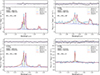 |
Fig. A.1. Fit of the Hα, [N II], and [S II] complex including both a broad and a narrow components of the Hα emission line, as is described in Sect. 2.2. The global fit is presented in red, while the narrow and broad Hα components are in green and yellow, respectively. The blue line represents the fit of the narrow [N II] doublet. In the upper panel are shown the residuals of the fit compared with the distribution of the 1σ (blue) and 3σ (red) errors on the fluxes. On the upper left part of the plots are reported the id, redshift, FWHMs derived from the fits, and the difference between the BIC value computed from the narrow-only line fit and the one from the fit with the additional broad Hα component |
Appendix B: CIGALE SED fitting parameters grid
Here we report the grid of parameters used for the SED-fitting with CIGALE described in Sect. 2.4
CIGALE parameters used for the SED fitting.
Appendix C: Final narrow-line AGN table
List of NLAGN selected in this work among CEERS MR spectra.
Appendix D: Spectra of the NLAGN at z > 6
Here, we report the 1D and 2D spectra of the NLAGN selected at z > 6.
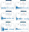 |
Fig. D.1. Spectra of the sources selected as NLAGN at z > 6. In each plot, we highlight in the box the main spectral features that led to the identification as a NLAGN (showing both the 1D and 2D spectrum). CEERS-613, CEERS-1019, CEERS-23 and CEERS-496 are marked only as tentative selections. The first because of the dubious He II λ1640 line in the 2D spectrum, while the other because of their dubious position in the diagnostic diagrams reported in Sect. 3 |
All Tables
All Figures
|
Fig. 1. Stacked spectra of the final sample of NLAGNs (red) and non-AGNs (blue) derived in the manner described in Sect. 2.3. We also marked the positions of some relevant lines. |
| In the text | |
|
Fig. 2. Left: R3N2 diagnostic diagram (also called BPT). The gray points represent the parent sample of galaxies analyzed in this work. Gold, green and red colors are used, respectively, for X-ray detected sources, radio-detected sources, and the high-z BLAGNs reported in Harikane et al. (2023). The NLAGNs selected using this diagram are marked with magenta edges. In magenta and cyan, we show the line ratios derived from the stacked spectra of all the selected NLAGN (52 sources) and non-AGN sources. The dashed lines refer to three different demarcation lines, as labeled, the one in green is the more conservative demarcation line derived in Scholtz et al. (2025). The shaded blue and red area represents the regions covered by the SFG and AGN photoionization models computed in Gutkin et al. (2016) and Feltre et al. (2016). The gray contours mark the distribution of SDSS sources (taken from SDSS DR7; Abazajian et al. 2009). In the lower-right corner are reported the median errors of the sample. Right: R3S2 diagnostic diagram (also called VO87) with the demarcation line originally presented in Kewley et al. (2001) (in black) and the new (more conservative) demarcation derived in Scholtz et al. (2025). Bottom: R3O1 diagnostic diagram with the demarcation line presented in Kewley et al. (2001) (dashed black line) and the new one derived in this work (solid green line). |
| In the text | |
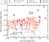 |
Fig. 3. He2N2 diagnostic diagram. The colors follow the same scheme as in Fig. 2 |
| In the text | |
|
Fig. 4. M1 and M2 diagnostic diagrams, firstly presented and discussed in Mazzolari et al. (2024). The colors follow the same scheme as in Fig. 2. |
| In the text | |
|
Fig. 5. C3He2 versus C43 diagnostic diagrams, selecting only one NLAGN due to the difficulties in detecting rest-UV lines in high-z galaxies with the short exposure times of the CEERS survey. The stacking line ratios and the average errors are not reported because of the poor statistics. The colors follow the same scheme as in Fig. 2. The demarcation lines are those defined in Hirschmann et al. (2023). |
| In the text | |
|
Fig. 6. From top to the bottom: C3He2 versus N4C3, C3He2 versus N5C3, C3He2 versus Ne4C3 diagnostic diagrams. The stacking line rations and the average errors are not reported because of the poor statistics. The colors follow the same scheme as in Fig. 2. |
| In the text | |
|
Fig. 7. Summarizing plots of the NLAGN selection. Upper: NLAGN counts in the different redshift bins, color-coded by the number of diagnostics in which each NLAGN has been selected. Lower: Distribution of the NLAGN according to the different diagnostic diagrams presented in Sect. 3, as labeled. |
| In the text | |
|
Fig. 8. Fraction of the spectroscopically selected NLAGN with respect to the parent sample in this work (CEERS, in red) and in the JADES survey (green) (program ID 1210&3215, Scholtz et al. 2025) in different redshift bins. The errors account for the statistical uncertainties and are computed considering a Poissonian noise. |
| In the text | |
|
Fig. 9. Redshift distribution of the intrinsic [O III] λ5007 line FWHM, resulting from the line-fitting procedure and subtracting the instrumental FWHM. On the left, we also report the median values of the FWHM of NLAGN (magenta), non-AGN (cyan) and of the global population (black) in five different redshift bins. Errors are derived using a bootstrap procedure. There is no significant trend of the FWHM of the sources with redshift. On the right, we report the histogram of the NL-FWHM distribution for AGN (red) and non-AGN (blue). |
| In the text | |
|
Fig. 10. Redshift distribution of the values of AV inferred from the Balmer decrement in sources with detected Hα and Hβ lines. For sources with upper limits on Hβ we derived lower limits on AV. On the left, we also report the median values of AV for NLAGN (magenta), non-AGN (cyan) and for the global population (black) in four different redshift bins. Errors are derived using the bootstrap procedure. On the right, we report the histogram of the AV distribution for AGN (red) and non-AGN (blue). |
| In the text | |
|
Fig. 11. Bolometric luminosities versus redshift of the sample of NLAGN selected in this work (red squares) compared to the bolometric luminosities of other AGN samples selected using JWST spectroscopic observations or pre-JWST, as labeled. The darker red squares represent the baseline bolometric luminosities, derived using Netzer (2009) calibration, while the fainter red squares show the values of the bolometric luminosities obtained using the same calibration adopted in Scholtz et al. (2025). The compilation of JWST selected BLAGN includes the sources taken from Maiolino et al. (2024b), Harikane et al. (2023), Matthee et al. (2024), Übler et al. (2023), Kocevski et al. (2023). SDSS BLAGN at z > 3 (light blue crosses) are taken from Wu & Shen (2022). AGN from the KASHz and SUPER surveys at Cosmic Noon (gray and red gold crosses) are taken from Harrison et al. (2016) and Kakkad et al. (2020), respectively. QSOs samples at Epoch of Reionization are taken from Zappacosta et al. (2023) (green crosses, HYPERION sample), and Mazzucchelli et al. (2023) (dark-blue crosses, XQR-30). |
| In the text | |
|
Fig. 12. Redshift distribution of the ratio between the SFR derived from the SED-fitting and the SFR computed from the MS relation derived by Popesso et al. (2023) at the redshift and M* of each source. We plot AGN and non-AGN sources with stars and circles, respectively. The sources are color-coded based on the stellar mass, as derived from the SED-fitting. |
| In the text | |
|
Fig. 13. 30″×30″cutouts of the X-ray stacking image in the observed SB (0.5–2 keV) and HB (2–8 keV) of the three samples taken into account. From top to bottom: BLAGNs, NLAGNs at z > 4.5, and NLAGNs at z < 4.5. None of the samples show a detection in either band. |
| In the text | |
|
Fig. 14. Results coming from the X-ray stacking, showing a significant X-ray weakness of all three samples of NLAGNs at z < 4.5, NLAGNs at z > 4.5, and high-z BLAGNs. Left: Expected X-ray luminosity versus observed X-ray luminosity (in the 2–10 keV band) of the three AGN samples we used for the stacking, as labeled. We also plot the sources in the CEERS MR sample with an X-ray detection color-coded by their obscuration level, as derived from the X-ray spectral analysis (Buchner et al. 2015). Diamonds refer to observed X-ray luminosities, while circles refer to the intrinsic X-ray luminosities derived from the X-ray analysis. Errors bars mark the error on the intrinsic X-ray luminosities of the sources reported in Buchner et al. (2015). The result from the X-ray stacking of these X-ray detected sources is reported as a gold diamond, while the gold circle considers the median of the intrinsic X-ray luminosities of the X-ray sources. The dashed lines correspond to the shift from the observed to intrinsic X-ray luminosities. In cyan, we report the z = 1.037 BLAGN CEERS-3129, presented in Appendix A. Right: Ratio between the mean bolometric luminosity of the three AGN samples (derived using the values computed in Sect. 4.7) and the observed X-ray luminosity upper limits versus the mean bolometric luminosities. The orange line shows the reference L2 − 10 keV − Lbol relation derived by Duras et al. (2020) and used to derive the expected X-ray luminosity of the sources. The empty hexagons represent the lower limits derived from the X-ray stack of the JWST-selected BLAGNs (red) and NLAGNs (green for z > 3 and blue for z < 3) on the CDFS and CDFN (Maiolino et al. 2025). |
| In the text | |
|
Fig. 15. Median radio stacking of the three AGN samples taken into account. From top to bottom, we report 25″×25″cutouts of BLAGNs, NLAGNs at z > 4.5, and NLAGNs at z < 4.5. None of the samples show radio detection. For each stack, we report the noise (rms) value in the top right corner. |
| In the text | |
|
Fig. 16. Expected 1.4 GHz radio luminosity versus observed radio luminosity from the stack of the three AGN samples, as labeled. The diamonds refer to the assumption that AGN are RQ, while circles to the hypothesis that sources are RL. We also show the positions of the single sources according to the color of the respective sample. With a cyan diamond, we report the z = 1.037 BLAGN CEERS-3129 (presented in Appendix A). The purple diamond represents the position of CEERS-2900 with the expected L1.4GHz derived using the RQ AGN relation, while the purple circle marks the expected L1.4GHz derived using the RL AGN relation. The shaded gray region represents the dispersion of the L1.4GHz − L2 − 10keV luminosity relation derived for radio-quiet AGN by D’Amato et al. (2022). |
| In the text | |
|
Fig. A.1. Fit of the Hα, [N II], and [S II] complex including both a broad and a narrow components of the Hα emission line, as is described in Sect. 2.2. The global fit is presented in red, while the narrow and broad Hα components are in green and yellow, respectively. The blue line represents the fit of the narrow [N II] doublet. In the upper panel are shown the residuals of the fit compared with the distribution of the 1σ (blue) and 3σ (red) errors on the fluxes. On the upper left part of the plots are reported the id, redshift, FWHMs derived from the fits, and the difference between the BIC value computed from the narrow-only line fit and the one from the fit with the additional broad Hα component |
| In the text | |
|
Fig. D.1. Spectra of the sources selected as NLAGN at z > 6. In each plot, we highlight in the box the main spectral features that led to the identification as a NLAGN (showing both the 1D and 2D spectrum). CEERS-613, CEERS-1019, CEERS-23 and CEERS-496 are marked only as tentative selections. The first because of the dubious He II λ1640 line in the 2D spectrum, while the other because of their dubious position in the diagnostic diagrams reported in Sect. 3 |
| In the text | |
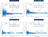 |
Fig. D.2. Continuation of Figure D.1 |
| In the text | |
Current usage metrics show cumulative count of Article Views (full-text article views including HTML views, PDF and ePub downloads, according to the available data) and Abstracts Views on Vision4Press platform.
Data correspond to usage on the plateform after 2015. The current usage metrics is available 48-96 hours after online publication and is updated daily on week days.
Initial download of the metrics may take a while.