| Issue |
A&A
Volume 700, August 2025
|
|
|---|---|---|
| Article Number | A104 | |
| Number of page(s) | 26 | |
| Section | Extragalactic astronomy | |
| DOI | https://doi.org/10.1051/0004-6361/202453534 | |
| Published online | 12 August 2025 | |
Euclid: Early Release Observations of diffuse stellar structures and globular clusters as probes of the mass assembly of galaxies in the Dorado group⋆
1
Université de Strasbourg, CNRS, Observatoire astronomique de Strasbourg, UMR 7550, 67000 Strasbourg, France
2
Institute of Astronomy, University of Cambridge, Madingley Road, Cambridge CB3 0HA, UK
3
INAF-Osservatorio di Astrofisica e Scienza dello Spazio di Bologna, Via Piero Gobetti 93/3, 40129 Bologna, Italy
4
Sterrenkundig Observatorium, Universiteit Gent, Krijgslaan 281 S9, 9000 Gent, Belgium
5
Institut universitaire de France (IUF), 1 rue Descartes, 75231 PARIS CEDEX 05, France
6
Laboratoire d’Astrophysique de Bordeaux, CNRS and Université de Bordeaux, Allée Geoffroy St. Hilaire, 33165 Pessac, France
7
INAF – Osservatorio Astronomico d’Abruzzo, Via Maggini, 64100 Teramo, Italy
8
INAF-Osservatorio Astronomico di Trieste, Via G. B. Tiepolo 11, 34143 Trieste, Italy
9
Université Paris-Saclay, Université Paris Cité, CEA, CNRS, AIM, 91191 Gif-sur-Yvette, France
10
INAF-Osservatorio Astronomico di Roma, Via Frascati 33, 00078 Monteporzio Catone, Italy
11
Observatorio Nacional, Rua General Jose Cristino, 77-Bairro Imperial de Sao Cristovao, Rio de Janeiro 20921-400, Brazil
12
Max Planck Institute for Extraterrestrial Physics, Giessenbachstr. 1, 85748 Garching, Germany
13
Institute for Astronomy, University of Edinburgh, Royal Observatory, Blackford Hill, Edinburgh EH9 3HJ, UK
14
European Southern Observatory, Karl-Schwarzschild-Str. 2, 85748 Garching, Germany
15
INAF-Osservatorio Astrofisico di Arcetri, Largo E. Fermi 5, 50125 Firenze, Italy
16
Department of Astrophysics/IMAPP, Radboud University, PO Box 9010 6500 GL Nijmegen, The Netherlands
17
Leiden Observatory, Leiden University, Einsteinweg 55, 2333 CC Leiden, The Netherlands
18
Universität Innsbruck, Institut für Astro- und Teilchenphysik, Technikerstr. 25/8, 6020 Innsbruck, Austria
19
Institute of Physics, Laboratory of Astrophysics, Ecole Polytechnique Fédérale de Lausanne (EPFL), Observatoire de Sauverny, 1290 Versoix, Switzerland
20
Visiting Fellow, Clare Hall, University of Cambridge, Cambridge, UK
21
Kapteyn Astronomical Institute, University of Groningen, PO Box 800 9700 AV Groningen, The Netherlands
22
Space physics and astronomy research unit, University of Oulu, Pentti Kaiteran katu 1, FI-90014 Oulu, Finland
23
Max-Planck-Institut für Astronomie, Königstuhl 17, 69117 Heidelberg, Germany
24
Department of Physics, Université de Montréal, 2900 Edouard Montpetit Blvd, Montréal, Québec H3T 1J4, Canada
25
Ciela Institute – Montréal Institute for Astrophysical Data Analysis and Machine Learning, Montréal, Québec, Canada
26
Mila – Québec Artificial Intelligence Institute, Montréal, Québec, Canada
27
Universitäts-Sternwarte München, Fakultät für Physik, Ludwig-Maximilians-Universität München, Scheinerstrasse 1, 81679 München, Germany
28
ESAC/ESA, Camino Bajo del Castillo, s/n., Urb. Villafranca del Castillo, 28692 Villanueva de la Cañada, Madrid, Spain
29
INAF-Osservatorio Astronomico di Brera, Via Brera 28, 20122 Milano, Italy
30
IFPU, Institute for Fundamental Physics of the Universe, via Beirut 2, 34151 Trieste, Italy
31
INFN, Sezione di Trieste, Via Valerio 2, 34127 Trieste, TS, Italy
32
SISSA, International School for Advanced Studies, Via Bonomea 265, 34136 Trieste, TS, Italy
33
Dipartimento di Fisica e Astronomia, Università di Bologna, Via Gobetti 93/2, 40129 Bologna, Italy
34
INFN-Sezione di Bologna, Viale Berti Pichat 6/2, 40127 Bologna, Italy
35
INAF-Osservatorio Astronomico di Padova, Via dell’Osservatorio 5, 35122 Padova, Italy
36
Centre National d’Etudes Spatiales – Centre spatial de Toulouse, 18 avenue Edouard Belin, 31401 Toulouse Cedex 9, France
37
Dipartimento di Fisica, Università di Genova, Via Dodecaneso 33, 16146 Genova, Italy
38
INFN-Sezione di Genova, Via Dodecaneso 33, 16146 Genova, Italy
39
Department of Physics “E. Pancini”, University Federico II, Via Cinthia 6, 80126 Napoli, Italy
40
INAF-Osservatorio Astronomico di Capodimonte, Via Moiariello 16 80131 Napoli, Italy
41
INFN section of Naples, Via Cinthia 6, 80126 Napoli, Italy
42
Dipartimento di Fisica, Università degli Studi di Torino, Via P. Giuria 1, 10125 Torino, Italy
43
INFN-Sezione di Torino, Via P. Giuria 1, 10125 Torino, Italy
44
INAF-Osservatorio Astrofisico di Torino, Via Osservatorio 20, 10025 Pino Torinese (TO), Italy
45
INAF-IASF Milano, Via Alfonso Corti 12, 20133 Milano, Italy
46
Centro de Investigaciones Energéticas, Medioambientales y Tecnológicas (CIEMAT), Avenida Complutense 40, 28040 Madrid, Spain
47
Port d’Informació Científica, Campus UAB, C. Albareda s/n, 08193 Bellaterra (Barcelona), Spain
48
Institute for Theoretical Particle Physics and Cosmology (TTK), RWTH Aachen University, 52056 Aachen, Germany
49
Institute of Cosmology and Gravitation, University of Portsmouth, Portsmouth PO1 3FX, UK
50
Dipartimento di Fisica e Astronomia “Augusto Righi” – Alma Mater Studiorum Università di Bologna, Viale Berti Pichat 6/2, 40127 Bologna, Italy
51
Instituto de Astrofísica de Canarias, Calle Vía Láctea s/n, 38204 San Cristóbal de La Laguna, Tenerife, Spain
52
Jodrell Bank Centre for Astrophysics, Department of Physics and Astronomy, University of Manchester, Oxford Road, Manchester M13 9PL, UK
53
European Space Agency/ESRIN, Largo Galileo Galilei 1, 00044 Frascati, Roma, Italy
54
Université Claude Bernard Lyon 1, CNRS/IN2P3, IP2I Lyon, UMR 5822, Villeurbanne F-69100, France
55
Institut de Ciències del Cosmos (ICCUB), Universitat de Barcelona (IEEC-UB), Martí i Franquès 1, 08028 Barcelona, Spain
56
Institució Catalana de Recerca i Estudis Avançats (ICREA), Passeig de Lluís Companys 23, 08010 Barcelona, Spain
57
UCB Lyon 1, CNRS/IN2P3, IUF, IP2I Lyon, 4 rue Enrico Fermi, 69622 Villeurbanne, France
58
Department of Astronomy, University of Geneva, ch. d’Ecogia 16, 1290 Versoix, Switzerland
59
INFN-Padova, Via Marzolo 8, 35131 Padova, Italy
60
INAF-Istituto di Astrofisica e Planetologia Spaziali, via del Fosso del Cavaliere, 100, 00100 Roma, Italy
61
Space Science Data Center, Italian Space Agency, via del Politecnico snc, 00133 Roma, Italy
62
FRACTAL S.L.N.E., calle Tulipán 2, Portal 13 1A, 28231 Las Rozas de Madrid, Spain
63
Dipartimento di Fisica “Aldo Pontremoli”, Università degli Studi di Milano, Via Celoria 16, 20133 Milano, Italy
64
Institute of Theoretical Astrophysics, University of Oslo, P.O. Box 1029 Blindern 0315 Oslo, Norway
65
Jet Propulsion Laboratory, California Institute of Technology, 4800 Oak Grove Drive, Pasadena, CA 91109, USA
66
Felix Hormuth Engineering, Goethestr. 17, 69181 Leimen, Germany
67
Technical University of Denmark, Elektrovej 327, 2800 Kgs. Lyngby, Denmark
68
Cosmic Dawn Center (DAWN), Copenhagen, Denmark
69
Institut d’Astrophysique de Paris, UMR 7095, CNRS, and Sorbonne Université, 98 bis boulevard Arago, 75014 Paris, France
70
NASA Goddard Space Flight Center, Greenbelt, MD 20771, USA
71
Department of Physics and Helsinki Institute of Physics, Gustaf Hällströmin katu 2, 00014 University of Helsinki, Finland
72
Aix-Marseille Université, CNRS/IN2P3, CPPM, Marseille, France
73
Université de Genève, Département de Physique Théorique and Centre for Astroparticle Physics, 24 quai Ernest-Ansermet, CH-1211 Genève 4, Switzerland
74
Department of Physics, P.O. Box 64 00014 University of Helsinki, Finland
75
Helsinki Institute of Physics, Gustaf Hällströmin katu 2, University of Helsinki, Helsinki, Finland
76
Aix-Marseille Université, CNRS, CNES, LAM, Marseille, France
77
NOVA optical infrared instrumentation group at ASTRON, Oude Hoogeveensedijk 4, 7991PD Dwingeloo, The Netherlands
78
University of Applied Sciences and Arts of Northwestern Switzerland, School of Engineering, 5210 Windisch, Switzerland
79
Universität Bonn, Argelander-Institut für Astronomie, Auf dem Hügel 71, 53121 Bonn, Germany
80
INFN-Sezione di Roma, Piazzale Aldo Moro, 2 – c/o Dipartimento di Fisica, Edificio G. Marconi, 00185 Roma, Italy
81
Dipartimento di Fisica e Astronomia “Augusto Righi” – Alma Mater Studiorum Università di Bologna, via Piero Gobetti 93/2, 40129 Bologna, Italy
82
Department of Physics, Institute for Computational Cosmology, Durham University, South Road, Durham DH1 3LE, UK
83
Université Paris Cité, CNRS, Astroparticule et Cosmologie, 75013 Paris, France
84
CNRS-UCB International Research Laboratory, Centre Pierre Binetruy, IRL2007, CPB-IN2P3, Berkeley, USA
85
Institut de Física d’Altes Energies (IFAE), The Barcelona Institute of Science and Technology, Campus UAB, 08193 Bellaterra (Barcelona), Spain
86
School of Mathematics and Physics, University of Surrey, Guildford, Surrey GU2 7XH, UK
87
European Space Agency/ESTEC, Keplerlaan 1, 2201 AZ Noordwijk, The Netherlands
88
DARK, Niels Bohr Institute, University of Copenhagen, Jagtvej 155, 2200 Copenhagen, Denmark
89
Waterloo Centre for Astrophysics, University of Waterloo, Waterloo, Ontario N2L 3G1, Canada
90
Department of Physics and Astronomy, University of Waterloo, Waterloo, Ontario N2L 3G1, Canada
91
Perimeter Institute for Theoretical Physics, Waterloo, Ontario N2L 2Y5, Canada
92
Institute of Space Science, Str. Atomistilor, nr. 409 Măgurele, Ilfov 077125, Romania
93
Dipartimento di Fisica e Astronomia “G. Galilei”, Università di Padova, Via Marzolo 8, 35131 Padova, Italy
94
Departamento de Física, FCFM, Universidad de Chile, Blanco Encalada 2008, Santiago, Chile
95
Institut d’Estudis Espacials de Catalunya (IEEC), Edifici RDIT, Campus UPC, 08860 Castelldefels, Barcelona, Spain
96
Satlantis, University Science Park, Sede Bld 48940, Leioa-Bilbao, Spain
97
Institute of Space Sciences (ICE, CSIC), Campus UAB, Carrer de Can Magrans, s/n, 08193 Barcelona, Spain
98
Departamento de Física, Faculdade de Ciências, Universidade de Lisboa, Edifício C8, Campo Grande, PT1749-016 Lisboa, Portugal
99
Instituto de Astrofísica e Ciências do Espaço, Faculdade de Ciências, Universidade de Lisboa, Tapada da Ajuda, 1349-018 Lisboa, Portugal
100
Universidad Politécnica de Cartagena, Departamento de Electrónica y Tecnología de Computadoras, Plaza del Hospital 1, 30202 Cartagena, Spain
101
Institut de Recherche en Astrophysique et Planétologie (IRAP), Université de Toulouse, CNRS, UPS, CNES, 14 Av. Edouard Belin, 31400 Toulouse, France
102
Infrared Processing and Analysis Center, California Institute of Technology, Pasadena, CA 91125, USA
103
Centre for Information Technology, University of Groningen, P.O. Box 11044 9700 CA Groningen, The Netherlands
104
INAF, Istituto di Radioastronomia, Via Piero Gobetti 101, 40129 Bologna, Italy
105
INFN-Bologna, Via Irnerio 46, 40126 Bologna, Italy
106
Aurora Technology for European Space Agency (ESA), Camino bajo del Castillo, s/n, Urbanizacion Villafranca del Castillo, Villanueva de la Cañada, 28692 Madrid, Spain
107
Institut d’Astrophysique de Paris, 98bis Boulevard Arago, 75014 Paris, France
108
ICL, Junia, Université Catholique de Lille, LITL, 59000 Lille, France
⋆⋆ Corresponding author: This email address is being protected from spambots. You need JavaScript enabled to view it.
Received:
19
December
2024
Accepted:
23
June
2025
Abstract
Deep surveys have helped to unveil the history of past and present galaxy mergers, and, in particular, uncovering their tidal debris and co-located globular clusters (GCs). Euclid’s unique combination of capabilities (spatial resolution, depth, and wide sky coverage) will make it a groundbreaking tool for galactic archaeology in the Local Universe, bringing low-surface-brightness (LSB) science into the era of large-scale astronomical surveys. Euclid’s Early Release Observations (ERO) demonstrate this potential with a field of view that includes several galaxies in the Dorado group. In this paper, we aim to derive from this image a mass assembly scenario for its main galaxies: NGC 1549, NGC 1553, and NGC 1546. We detected their internal and external diffuse structures, and identified candidate GCs. By analysing the colours and distributions of the diffuse structures and candidate GCs, we can place constraints on the galaxies’ mass assembly and merger histories. The results demonstrate that feature morphology, surface brightness, colours, and GC density profiles are consistent with galaxies that have undergone different merger scenarios. We classify NGC 1549 as a pure elliptical galaxy that has undergone a major merger. NGC 1553 appears to have recently transitioned from a late-type galaxy to early type, after a series of radial minor to intermediate mergers. NGC 1546 is a rare specimen of galaxy with an undisturbed disk and a prominent diffuse stellar halo, which we infer has been fed by minor mergers and then disturbed by the tidal effect from NGC 1553. Finally, we identify limitations specific to the observing conditions of this ERO, in particular, stray light in the visible and persistence in the near-infrared bands. Once these issues are addressed and the extended emission from LSB objects is preserved by the data-processing pipeline, the Euclid Wide Survey will allow for studies of the Local Universe to be extended to statistical ensembles over a large part of the extragalactic sky.
Key words: galaxies: interactions / galaxies: groups: individual: Dorado / galaxies: star clusters: general / galaxies: structure
This paper is published on behalf of the Euclid Consortium.
Deceased.
© The Authors 2025
 Open Access article, published by EDP Sciences, under the terms of the Creative Commons Attribution License (https://creativecommons.org/licenses/by/4.0), which permits unrestricted use, distribution, and reproduction in any medium, provided the original work is properly cited.
This article is published in open access under the Subscribe to Open model. This email address is being protected from spambots. You need JavaScript enabled to view it. to support open access publication.
1. Introduction
The dark energy, cold dark matter standard model, coupled with hierarchical mass assembly theory, suggests that galaxies originate from the agglomeration of baryonic matter within small and low-mass dark matter halos in the early Universe (e.g. Dekel & Silk 1986; Klypin et al. 1999; Moore et al. 1999). According to this paradigm, one of the galaxy mass accretion channels is via the mergers they have undergone during their history (e.g. Conselice 2014; Somerville & Davé 2015). These events are known to have several repercussions on the resultant galaxies. Key outcomes of such mergers could include an increase in the activity of an active galactic nucleus (e.g. Sanders & Mirabel 1996; Ellison et al. 2019), interactions between the central black holes of the progenitors leading to a binary and, possibly, a fusion (e.g. Koss et al. 2023; Blumenthal & Barnes 2018), and the initiation of starbursts due to the collision of gas clouds from the merging galaxies (e.g. Barnes 2004; Kim et al. 2009; Saitoh et al. 2009; Renaud et al. 2022). These processes often result in morphological changes, primarily due to a violent relaxation of the stars and tidal effects. Those tidal effects produce a wealth of debris and extended stellar structures around galaxies.
Among those debris, tidal tails, which are large elongations on either side of a galaxy, are the most well known through particularly illustrative systems such as the Antennae galaxies (e.g. Lahén et al. 2018). Such structures appear during a major merger. Tails can appear as bridges between two interacting galaxies in the early phase of the merger, or less elongated ‘plumes’ when the progenitors are of early type (e.g. Arp 1966; Toomre & Toomre 1972; Mihos et al. 1995). Stellar streams are the tidal tails of satellites which have been disrupted and then accreted by their host galaxy. They are thus witnesses of minor mergers (e.g. Bullock & Johnston 2005; Belokurov et al. 2006; Ibata et al. 2021; Martin et al. 2022). Finally, shells are shaped like arcs, usually sharing the same centre as the galaxy. They form during radial collisions, when galactic material is expelled radially (e.g. Quinn 1984; Prieur 1990). Cosmological simulations show that tidal features disappear by phase-mixing after two to eight billion years (e.g. Pop et al. 2018; Mancillas et al. 2019).
Diffuse stellar features, including extended halos, can be traced by individual compact sources that are related to them: red giant branch and asymptotic giant branch stars, H II regions, planetary nebulae, and globular clusters (GCs), enabling their chemo-dynamical mapping (e.g. Cohen 2000; Durrell et al. 2003; Coccato et al. 2009; Usher et al. 2012; Pota et al. 2013; Greggio et al. 2014; Voggel et al. 2016; Koch et al. 2018; Rejkuba et al. 2022; Hartke et al. 2022). Recent studies observed GC alignment and dynamics along tidal features for various galactic systems in the Local Universe, including M31 (Mackey et al. 2010, 2019; Veljanoski et al. 2013; Huxor et al. 2014), NGC 4651 (Foster et al. 2014), NGC 0474 2017ApJ...835..123L, and NGC 5128 (Hughes et al. 2021). These works have led to the detection of several GCs associated with tails, streams, and shells. Nevertheless, the use of GC clustering for detecting tidal features remains to be proven.
For more distant Local Universe galaxies not resolved into stars, tidal features appear in the form of diffuse structures that may be faint in terms of stellar surface brightness. Noteworthy contributions for unveiling the low-surface-brightness (LSB) Universe include both amateur (e.g. Martínez-Delgado et al. 2010; Karachentsev et al. 2015; Javanmardi et al. 2016; Mosenkov et al. 2020) and professional facilities (e.g. Merritt et al. 2014; Greco et al. 2018; Borlaff et al. 2019; Müller et al. 2019; Carlsten et al. 2022; Paudel et al. 2023). Examples worth mentioning are the Dragonfly telephoto array (e.g. Abraham & van Dokkum 2014), the Hyper Suprime-Cam Subaru Strategic Program (HSC-SSP) (e.g. Aihara et al. 2017), the Large Binocular Telescope (Smallest Scale of Hierarchy survey: Annibali et al. 2020; LBT Imaging of Galactic Halos and Tidal Structures: Trujillo et al. 2021), the Sloan Digital Sky Survey (SDSS; e.g. York et al. 2000; Belokurov et al. 2006; Morales et al. 2018), the Dark Energy Spectroscopic Instrument (DESI) Legacy imaging surveys (e.g. the Dark Energy Camera Legacy Survey [DECaLS]; Dey et al. 2019), the 2 m Fraunhofer Wendelstein Telescope (Hopp et al. 2014; Kluge et al. 2020; Zöller et al. 2024), and the VLT Survey Telescope (VST) Early-type GAlaxy Survey (VEGAS; Capaccioli et al. 2015) as well as research conducted at the Canada-France-Hawaii Telescope (Mass Assembly of early-Type GaLAxies with their fine Structures, MATLAS: Duc et al. 2015; Bílek et al. 2020, Canada-France Imaging Survey CFIS: Ibata et al. 2017, Next Generation Virgo Cluster Survey NGVS: Ferrarese et al. 2012). Several future projects will be compatible with LSB studies, taking this science into the era of large-scale surveys. These include the Vera Rubin Observatory (Ivezić et al. 2019; Brough et al. 2020), Nancy Roman Grace Space Telescope (Koekemoer & Roman Deep Fields Working Group 2023; Montes et al. 2023), and ARRAKIHS (Guzmán 2024).
Euclid (Euclid Collaboration: Mellier et al. 2025), launched in July 2023, is leading a six-year cosmological mission to observe the extragalactic sky in a unique combination of spatial resolution, coverage, photometric bands, and depth. Its capabilities, particularly in terms of its detection limits in surface brightness and its high image resolution associated with a sharp point spread function (PSF), offer promising prospects of both tracing tidal features (Euclid Collaboration: Borlaff et al. 2022) and studying the distribution of GCs (e.g. Lançon et al. 2021; Euclid Collaboration: Voggel et al. 2025). The Euclid Wide Survey (EWS; Euclid Collaboration: Scaramella et al. 2022) thus raises the possibility to extend the study of both tidal features and GCs in numerous galactic systems and across an extensive area of the sky (nearly 14 000 deg2).
Euclid’s Early Release Observations (ERO) programme (Cuillandre et al. 2025) managed by the European Space Agency (ESA) provides a new perspective on numerous objects within the Local Universe, showcasing this telescope’s potential in LSB science and galactic archaeology across various scales. It spans from detecting tidal tails around Milky Way GCs (Massari et al. 2025) and dwarf galaxies of the Perseus galaxy cluster (Marleau et al. 2025) to investigating the intricacies of intra-cluster light (Kluge et al. 2025). Among the images acquired as part of the ERO programme, one pointing is well suited for investigation of surroundings of massive galaxies in Dorado, a rich galaxy group located at a distance of 17.7 Mpc (e.g. Huchra & Geller 1982; Firth et al. 2006; Kourkchi & Tully 2017). In the observed field of view (FoV), several early-type galaxies (ETGs; NGC 1549, NGC 1553, and NGC 1546) are particularly striking showcases of tidal distortions. In particular, NGC 1549 and NGC 1553 are known to form an interacting pair, and NGC 1546 displays also a system of tidal features (e.g. Malin & Carter 1983; Dupraz et al. 1987; Weil & Hernquist 1993).
Already on photographic plates, the NGC 1553 / NGC 1549 (S0 / E) pair was identified as hosting streamer and ripple features located at around and beyond a radius of 5′ from the centre of these galaxies (Freeman 1975; Jedrzejewski 1987; Bridges & Hanes 1990). The study of the central regions of those galaxies, presented in Ricci et al. (2023), reveals that NGC 1553 has a Low-Ionization Nuclear Emission-line Region (LINER) featuring a broad component, an X-ray core (She et al. 2017; Bi et al. 2020), and coronal [Ne V] emission in the mid-infrared (Rampazzo et al. 2013). The Sa galaxy NGC 1546 (Comerón et al. 2014) is located at a projected distance about 140 kpc from the pair and its tidal feature system has not been described in detail.
Rampazzo et al. (2020, 2021, 2022) investigated the star formation of the Dorado galaxies, comparing their emission in Hα (Las Campanas Observatory Hα[N II] narrow bands observations) and far-ultraviolet (Astrosat-UVIT FUV.CaF2 observations) with earlier research on their emission in H I (de Vaucouleurs et al. 1991; Kilborn et al. 2005), respectively. Those studies clarify why, among the three ETGs, only NGC 1546 has H I: dissipative events would have initiated star formation and exhausted the H I in NGC 1549 as in NGC 1553, whose far-ultraviolet emission are each associated with a disk structure. Additionally, far-ultraviolet imaging reveal NGC 1549, NGC 1553, and NGC 1546 inner and resonance rings and H II regions for NGC 1546 and NGC 1553. Unlike NGC 1549, which appears as a purely quenched elliptical galaxy, NGC 1553 has a star-formation rate above the average for ETGs, and presents star-forming clumps and rotation. Finally, Hubble Space Telescope and recent JWST images of NGC 1546 revealed its flocculent spiral galaxy nature.
Several hypotheses have been proposed to explain the position of these galaxies in the structure of the Dorado group (and its connection with the nearby clusters, Fornax and Eridanus; e.g. Raj et al. 2024). Garcia (1993) considered that NGC 1549 was associated with an independent group centred around NGC 1553, while later Kilborn et al. (2005) estimated both galaxies to be part of a group with NGC 1566 at its core. Also, Makarov & Karachentsev (2011) envisioned that NGC 1553 is one of the centres of two independent groups forming Dorado. Finally, Iovino (2002) presents NGC 1549, NGC 1553, and NGC 1546 as forming, with the edge-on late-type galaxy (LTG) IC 2058, the compact group SCG 0414−5559 at the barycentre of Dorado.
This paper focuses on the merging histories and current interactions of these galaxies, which are studied based on the analysis of their LSB stellar structures together with their GC populations. This study allows for the evaluation of the substantial benefits and limitations of Euclid for detection of LSB Local Universe objects that are not resolved into individual stars. The article is organised as follows. The Euclid ERO Dorado (ERO-D) data and the methods employed to investigate the galaxies’ past history are described in Sect. 2. Section 4 outlines the results associated with these analyses, with their limitations discussed in Sect. 5. A proposition of recent merger history for the ERO-D galaxies is also provided in this section, as well as prospects on Euclid detection. Our findings are summarised in Sect. 6.
2. Data
2.1. The ERO-D dataset
We used imaging data from the Euclid visible (VIS) instrument (Cropper et al. 2018; Euclid Collaboration: Cropper et al. 2025), employing the IE optical filter with a pixel scale of  and from the Near Infrared Spectrometer and Photometer (NISP) instrument (Euclid Collaboration: Schirmer et al. 2022; Euclid Collaboration: Jahnke et al. 2025), using the near-infrared (NIR) filters YE, JE, and HE, each with a pixel scale of
  . In this paper, we use the AB system and adopt the following convention: apparent magnitudes are denoted as IE, YE, JE, and HE, while the absolute magnitudes are denoted as MIE, MYE, MJE, and MHE.
ERO-D was observed in November 2023 using one reference observational sequence (ROS), namely four 560-second exposures in the IE filter and four 87.2-second exposures in each of the NISP instrument’s filters. This process mirrors the approach that will be adopted for the EWS, with the exception that a non-optimal position of the spacecraft with respect to the Sun makes the presence of significant stray light possible in the ERO-D IE image (Cuillandre et al. 2025).
The raw single exposures were processed through a dedicated pipeline, which produces the stacks used in this paper. This processing is described in Cuillandre et al. (2025), along with further detail about each ERO dataset. In particular, for ERO-D, the limiting surface brightness for extended emission, measured in mag arcsec−2 on a 10″ × 10″ scale (Román et al. 2020), is estimated as 30.05 in IE, 28.41 in YE, 28.58 in JE, and 28.60 in HE.
In Fig. 1, the ERO-D coverage (approximately  centred on
  ,
,  ) is shown in red. It notably includes four major galaxies of the Dorado group: NGC 1553, NGC 1549, NGC 1546, and IC 2058. The IE surface brightness map and the colour image of the Euclid ERO-D field is displayed in Fig. 2.
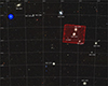 |
Fig. 1. DECaLS colour image of the Dorado group. The brightest members are labeled in the figure. The HEALPix Multi-Order Coverage map (Fernique et al. 2014) of the Euclid ERO-D FoV is added to the image as a red-transparent overlay. The coordinates are given in RA, Dec. |
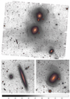 |
Fig. 2. Euclid surface brightness maps in the IE band with a scale in mag arcsec−2 indicated to the bottom. Colour images made by co-adding the IE, the YE, and the HE bands using Astropy (Astropy Collaboration 2013, 2018, 2022) are super-imposed in the inner regions of the main galaxies. Top: Whole FoV (≈56 arcmin2) of the ERO-D observations. Lower-left: 300″ × 300″ cutout around IC 2058 and the dwarf galaxy PGC 75125. Lower-right: 600″ × 600″ cutout around NGC 1546. In this figure, north is up, east is to the left. |
2.2. Diffuse light contaminants
The ERO-D observations were acquired with one single ROS and therefore share the same depth as the standard EWS. As such they may be used as a test-bed on the Euclid capability to detect and analyse extended LSB structures like tidal debris. In this subsection, we list the potential contaminants for each Euclid filter.
The instrument PSF is usually one of the main limiting factors in LSB studies (e.g. Sandin 2014; Abraham & van Dokkum 2014; Karabal et al. 2017). Indeed, in many studies using non-optimised cameras, the wings of the PSF introduce an additional, artificial diffuse component in the surrounding of every source, including extended galaxies. In this paper, for diffuse light photometry, we do not use deconvolution by an extended PSF of Euclid. Instead, we make careful decisions in terms of photometric methods (as described in Sect. 3) that minimise its impact (which is already limited due to its notable sharpness and the low level of its wings, according to Cuillandre et al. 2025). For more details regarding the impact of Euclid’s PSF and on the regimes for which omitting deconvolution when producing surface brightness profiles of nearby galaxies is possible, we refer the reader to Appendix B of Mondelin et al. (2025).
Euclid’s NISP instrument covers not only imaging in the YE, JE, and HE bands, but also acquisition of spectra using a grism, which creates artefacts on IR images. They take the form of parallel linear persistence charge features centred on bright objects. In areas of the image affected by persistence, measured photometry, and therefore colour, of LSB objects is less reliable. If masked incorrectly, these contaminants can also alter the surface brightness profiles of the outer regions of galaxies. The problem is partially corrected through modelling and subtraction during the ERO pipeline run (Cuillandre et al. 2025), but there are still sources that present this issue in the ERO-D FoV. In addition, the NIR images are subject to detector levels differences, which are still visible in the stacks. These two issues can hinder the detection of faint features, as shown in Fig. 3.
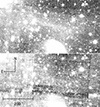 |
Fig. 3. Impact of varying detector sensitivities and persistence on tidal feature detection in NIR bands. Top: IE image centred on a diffuse feature at the north of NGC 1546. Bottom: Same field in HE, where the feature is much less visible. |
During the visual inspection of the IE image, we detect a large diffuse light component which affects mainly the southern part of the image, and reaches IC 2058 (see Fig. 2). There is no bright pattern in NIR that matches this diffuse emission in IE, which can, in principle, be explained by the lower depth of Euclid’s IR bands (and implies that no reliable colour information is available for this component). Three possible interpretation of this diffuse component were explored.
-
The presence of an intra-group light. Nevertheless, the shape of this emission areas seemed suspicious, tracing sometimes the boundaries of the CCDs.
-
Galactic cirrus within the ERO-D FoV. This type of structure can indeed take on characteristic shapes with preferred directions. However, checking IR images of the FoV region suggests that the risk of such contamination is limited: in Fig. 4, the WISE (Wright et al. 2010; Miville-Deschênes et al. 2016) data do not show such structures in the ERO-D FoV.
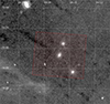
Fig. 4. View of the 12 μm photometric band of the WISE IR survey (reprocessed by Meisner & Finkbeiner 2014), allowing us to probe the presence of Galactic cirrus. The ERO-D FoV is displayed in semi-transparent red. The coordinates are given in RA, Dec.
-
Stray light contamination. Due to observing constrains during the ERO observations, the telescope was not oriented in a position minimising stray light (Cuillandre et al. 2025), as will be done for the regular Euclid survey.
The comparison and striking similarity of this diffuse emission with early, incomplete stray light maps from the first Euclid data (Schirmer & Soldano, priv. comm.) convinced us to favour the latter hypothesis throughout this article, although a combination of several of the previously described origins remains possible. This region should be the subject of a dedicated study on intra-group light once re-observed as part of the EWS.
3. Methods
3.1. Large-scale diffuse light component subtraction and comparison with ground-based data
Regardless of its nature, the large-scale diffuse light component may interfere with the individual photometry of smaller features, prompting us to create a large-scale diffuse light subtracted version of the IE image dedicated to this analysis.
In the absence of a model to subtract this large-scale diffuse component, we are opting for a local background approach. For this, we need to mask not only the galaxies but also their faint features, so that only the sky and large-scale diffuse light component remain unmasked. This can be achieved with MTObjects, a segmentation algorithm optimised for faint extended sources, based on a Max-Tree method (Teeninga et al. 2015); TeeningaMoschiniTragerWilkinson+2016. To obtain a mask, we run this software on the IE image, re-binned six times to enhance the signal-to-noise ratio (S/N) of the galaxy features (central panel of Fig. 5). During this step, MTObject is used with its default configuration, except for the move_factor which is set to 0, ensuring extensive masks. Finally, we calculate the local background on the original grid with the resampled MTObjects mask using the source-extractor (Bertin & Arnouts 1996) Python version sep (Barbary 2016) with a cell size of 100 pixels × 1000 pixels (≈1.7′×1.7′). The large-scale diffuse light component unmasked and above this scale is removed, and the background is flattened (right panel of Fig. 5). Although useful for the photometry of individual few arcminute-sized features, the corrected image might have removed real, very extended LSB stellar structures and cannot be used as a reference image for other tasks, such as calculating the photometric profile at large distances from the galaxy centre. The large-scale diffuse light subtracted image is therefore used solely for the photometry of smaller-scale individual structures and their qualitative comparison in colour maps. Additionally, in the following, we specify the use of the image with large-scale diffuse light subtracted by referring to it as the IE corrected image. We employ Gnuastro Astwarp (Akhlaghi & Ichikawa 2015) to create a version of the IE corrected image, which is reprojected on NIR images, ensuring alignment with the NIR bands’ pixel scale and grid.
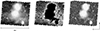 |
Fig. 5. Large-scale diffuse light component correction for the IE image. Left: Original IE image. Centre: sep background map. The MTObjects masks are in black. Right: sep local background-subtracted output IE image. |
To further investigate the instrumental contamination on the diffuse light, in particular the stray light, we compare the Euclid original IE image to non-background-subtracted data from the ground-based DECaLS survey, which fully covers the ERO-D region (tiles 412-5540, 413-5540, 417-5540, and 418-5622). We used the i band, which is close to the Euclid IE band (despite the latter covering also a part of the DECaLS r band and having a higher throughput). We subtract a constant background, and then co-add the DECaLS i images using GnuAstro AstWarp. We estimate the DECaLS i surface brightness map and finally subtract it from the Euclid IE surface brightness map. It is worth noting that ERO-D has a surface brightness limit (30.05 mag arcsec−2 for IE, Cuillandre et al. 2025) fainter than that of DECaLS (up to 29 mag arcsec−2, Miró-Carretero et al. 2023). Consequently, in the left panel of Fig. 6, the dark areas reveal both where Euclid detects more flux and features than DECaLS, and where Euclid is potentially still affected by stray light.
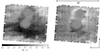 |
Fig. 6. Residual image subtracting the DECaLS i-band surface brightness map from the EuclidIE surface brightness map. The scale gives the residual in mag arcsec−2. Left: Residual image using the original IE image. The extended dark area in the lower part of the image indicates the possible presence of stray light. Right: Residual image using the IE corrected surface brightness map. |
The stray light issue has been noted for several data sets in the Euclid ERO programme (Cuillandre et al. 2025), leading to a redefinition of the orientation of the telescope during the EWS (Euclid Collaboration: Mellier et al. 2025). As a result, the impact of this source of contamination will be drastically reduced in the future data releases. In agreement with the middle panel of Fig. 5, we show in Fig. 6 that some diffuse halo-light was included in the local background map we used to construct our IE corrected image.
3.2. Identification and characterisation of tidal features and substructures
3.2.1. Cutouts and sources masking
We generated cutouts centred on each bright galaxy of interest and encapsulating its visible halo, stellar features, and enough sky area to estimate the background value for modelling and photometry. Specifically, the cutouts for galaxies NGC 1549 and NGC 1553 are created with a dimension of 1200″ × 1200″, whereas the cutout for NGC 1546 and IC 2058 are smaller, measuring 600″ × 600″ and 330″ × 330″, respectively.
We created a version of the IE original image which is reprojected on the pixel grid of the NIR bands, which is useful for the feature detection (since this process increases their S/N) and colour maps and profiles (see Sect. 3.2.3). Precise galaxy modelling requires masking all foreground stars and background galaxies in the FoV. Our method consists in producing binary masks with the help of segmentation maps of both cutouts and complete FoV images using the MTObjects tool.
3.2.2. Unsharp masking
We used unsharp masking to make the tidal features more prominent and to highlight internal structures. This technique involves subtracting a smoothed version of the initial image from the original. To prevent excessive subtraction in the innermost regions of the galaxies of interest, we started by creating an image with a flattened dynamic range. This was achieved by applying an asinh stretch to the original image. For each filter, we then subtracted a stretched, smoothed, and star-masked image from the stretched image.
3.2.3. Ellipse fitting, colours, and profiles
To model the major galaxies of the ERO-D FoV, we opted for an ellipse fitting approach. AutoProf (Stone et al. 2021) is an automated non-parametric ellipse fitting PYTHON tool that takes as inputs the cutouts and associated masks described in Sect. 3.2.1. We ran the software on the non-re-binned cutouts (for the IE band, we used the non-corrected image) to subtract a constant background and extract surface brightness profiles for the galaxies NGC 1549, NGC 1553, NGC 1546, and IC 2058. During this profile extraction process, all the parameters (centre, ellipticity, position angle) were allowed to vary, in order to achieve high-precision galaxy subtraction for each band.
We note that the galaxies NGC 1549 and NGC 1553 partially overlap. To avoid any issues related to this overlap, we performed their ellipse fitting in two steps. We first carry out an ellipse fitting for NGC 1553, allowing us to subtract this galaxy before performing the final ellipse fitting on NGC 1549. The opposite approach is applied when fitting NGC 1553. Subtracting the galaxy models, we obtain residuals images in the IE (both original and corrected), YE, JE, and HE bands.
Before examining the colours, we note that in this region of the sky, the extinction is negligible (Schlegel et al. 1998; Schlafly & Finkbeiner 2011). To examine the colour profiles of the main galaxies, we used AutoProf with the prepared cutouts and masks, this time using a forced photometry mode (i.e. the centre, ellipticity, and position angle are fixed to the values obtained for the IE-band profile). This choice facilitates the consistent comparison of surface brightness profiles across different bands. The final step involves subtracting the surface brightness profiles of one band from another, yielding colour profiles (in particular, IE − HE and IE − JE) for each galaxy.
In addition to colour profiles, we also generate 2D colour maps. In order to do this, we make use of the IE corrected image. We first estimate the background level for the full FoV, both rebinned IE and original JE, YE, and HE images. We make use of MTObjects masking and a method derived from the AutoProf algorithm, using as background value the first prominent peak of the smoothed histogram of pixel values of the image. We then constructed detailed surface brightness maps for each band by replacing flux with surface brightness in each pixel. The colour maps are produced by subtracting the pairs of surface brightness maps. It is worth noting that for the photometric results presented in this paper (both profiles and values), we propagated the uncertainty arising from the width of the first histogram peak used to determine the background.
3.2.4. Detecting, classifying, and characterising features with annotations
We used the Jafar annotation tool (Sola et al. 2022) to perform a visual inspection of the images and identification of tidal features. This online software enables users to navigate images, zoom in and out, and to draw the shapes of LSB features superimposed on deep images. In practice, it is necessary to precisely delineate the boundaries of each feature using polygonal shapes and assign labels, describing the type of the structure. Two other experts verify the final annotations visually. The coordinates of the contours and annotation labels are stored in a database, allowing for the subsequent retrieval of quantitative measurements and the creation of feature masks. The annotations are made taking into account the IE and colour images, but also ellipse fitting residual and unsharp masked images for probing the inner features.
The colour maps alone enable a qualitative study, but they are not representative of the individual feature photometry. Indeed, the galaxy models were not subtracted, so the colour of the features ends up mixed with that of the extended halos of these galaxies. It is then necessary to perform individual feature photometry, which heavily depends on local background variations near the studied structure. To minimise these variations, and thereby the uncertainty in the photometry of individual features, we used the IE corrected image.
We generated masks that precisely match the shape of each structure using the contours extracted from Jafar. To avoid flux contamination by the host galaxy, we used the ellipse fitting residual images to perform this photometry. We considered the remaining background to be flat.
For each feature and in each photometric band, we used a cutout that encompasses the structure and its immediate surroundings. We masked stars and distant galaxies using MTObjects and the tidal feature, using its contour extracted from the Jafar annotation tool. The background value estimation method that follows is similar to the one described in Sect. 3.2.3. To measure the feature integrated flux, small sources inside the structure have to be masked. For the segmentation step, MTObjects, which is optimised for more extended sources masking, is then replaced by sep. Its default parameters were used here, except thresh, which is set to 1.5, and err to the global background RMS.
3.3. Globular clusters (GCs)
3.3.1. GC identification
The spatial resolution of Euclid IE images, combined with the optical and NIR colours of Euclid, as well as the ground-based surveys, enables us to identify GC candidates within the ERO-D FoV. Additional information from the GCs, including their spatial distribution and colours, can provide further insights into investigating the mass assembly of the two interacting galaxies, NGC 1549 and NGC 1553, in this ERO field. We identified GCs in the FoV through several steps, including creating PSF models, source detection, photometry, injecting artificial GCs, and finally, selecting GC candidates. This procedure is similar to the methodology in Saifollahi et al. (2025a) for the Euclid ERO Fornax galaxy cluster (ERO-F) with some modifications to the colour selection. Furthermore, in this work, we also used g, r, and i band images from the Dark Energy Survey (DES; DES Collaboration 2021). The additional colour information provided by these images helps to reduce contamination from foreground stars and background compact sources.
We started the analysis by producing PSF models in all seven bands (four Euclid and three DES bands) using bright, non-saturated stars within the FoV. Next, we generated a multi-wavelength source catalogue with photometry in seven bands. Sources were detected by applying unsharp-masking on the original IE image (Saifollahi et al. 2025b) and using SExtractor with DETECT_THRESH = 1.5. We used similar SExtractor parameters as provided in Table 3 in Saifollahi et al. (2025a). Subsequently, forced aperture photometry was carried out using photutils (Bradley et al. 2016) in all bands at the given coordinates of the detected sources. In addition, we measured a compactness index of sources in IE within aperture diameters of two and four pixels (Peng et al. 2011). Here, the aperture photometry was done on background-subtracted images using a 12 pixel × 12 pixel background mesh size. Such a small mesh size is needed to estimate the local background close to the central regions of massive galaxies, where the slope of the light profile is changing rapidly; however, this mesh size does not influence the photometry of small sources by more than 1%. Based on our analysis of artificial GCs, the completeness of source detection in the IE band is above 98% at IE < 25 (which corresponds to the faintest GCs for a Gaussian globular cluster luminosity function (GCLF) around massive galaxies, Saifollahi et al. 2025a), with 80% and 50% completeness limits at IE = 25.4 and IE = 25.6, respectively. Later, for GC selection, we apply a compactness index, ellipticity, and various colour criteria to select GC candidates that will reduce completeness by 20%. We examined not only the completeness as a function of the magnitude, but also the completeness of source detection as a function of the location in the FoV (called spatial completeness hereafter). An initial visual inspection shows that outside the central 1 kpc of the main galaxies our detection procedure does not miss point sources. To further evaluate this, we conducted a straightforward test aimed at assessing the completeness of source detection by selecting foreground stars. We identified these stars across the FoV based on their full width at half maximum (FWHM) and IE − YE colour. Our analysis revealed that the distribution of stars was uniform throughout the frame. Furthermore, we evaluated the completeness of source detection within the ERO-D FoV using artificial GCs, and found a consistent level of spatial completeness for sources with IE < 24 in the field, including the regions around NGC 1553 and NGC 1549 (see Fig. 7).
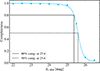 |
Fig. 7. GC completeness of ERO-D as a function of IE, SIM, the magnitude of artificial GCs injected in the data. Note: at the distance of the Dorado galaxies, real GCs are expected to be distributed between IE = 21 and IE = 25. |
In the next step, we performed the GC identification. We used the created PSF models and produce artificial GCs (using the King profile, King 1966) of sizes (half-light radius) between 2 pc and 5 pc, absolute IE magnitude between −11 and −5, and colours IE − YE = 0.45, YE − JE = 0.1, JE − HE = 0, g − r = 0.6, and g − i = 0.9. The artificial GCs are then distributed uniformly across the frames. Using the artificial GCs, we estimate the uncertainties in the measured parameters of GCs at a given magnitude. Given these uncertainties, we define flux-dependent selection criteria for compactness index (in IE), colours, and ellipticity (in IE) for GCs. These criteria select the artificial GCs within 5–95, 1–99, and 1–99 percentiles in compactness index, ellipticity and colours (5 colours), and overall, 80%. Taking into account the completeness in source detection (above 97%), our methodology selects 77% of the artificial GCs.
The scatter in the colours of the artificial GCs only takes into account the measurement uncertainty. For colour selection of GC candidates, we broaden the range of colours of the artificial GCs by the width of the colours for old GCs (older than 7 Gyr) with sub-solar metallicities (Z < 0.02) from stellar population models (See Appendix A in Saifollahi et al. 2025a). This broadening is the same across magnitude and is about ±0.3, ±0.15, ±0.15, ±0.3, and ±0.3 mag for IE − YE, YE − JE, JE − HE, g − r, and g − i, respectively. This means that for the fainter sources that are not detected in the DES bands, only Euclid bands and colours are used for colour selection. Once the GC candidates are selected, we continue with the analysis of GC distribution around galaxies and across the FoV of ERO-D, as well as their colours.
Lastly, considering that our analysis is based on artificial GCs with a half-light radius between 2 and 5 pc, we expected to miss those GCs that are smaller and larger than these limits. Based on the analysis of the ERO-F data in Saifollahi et al. (2025a), we expected at least 30% of the GCs to be too small to be resolved in Euclid IE images. Considering this, we expect an overall completeness of about 50% in the GC selection applied here, but this also depends on the properties of the GC population of each galaxy. For more details on the general method of GC selection and completeness estimation, we refer the reader to Saifollahi et al. (2025b).
3.3.2. From GC distribution to GC colours in features
To study the distribution of GCs over the ERO-D FoV, we generate density maps. We consider GC candidates verifying IE < 24, which is about 1 mag fainter than the turn-over magnitude of the GCLF (based on the GCLF for massive galaxies in Fig. 14 of Saifollahi et al. 2025a which peaks at IE ≈ 23 mag, see also Harris 2001; Rejkuba 2012). We therefore reduce the number of contaminant sources (non-GCs), which increase at the fainter magnitudes (Saifollahi et al. 2025a). In the following, we refer to this set as the ‘bright GC candidates’. Isodensity contours can then be easily obtained from the catalogue using the gaussian_kde function from the SciPy Python package. The kernel bandwidth to obtain the smoothed distribution respects the Scott’s rule, described in Eq. (1) as
 (1)
(1)
where h is the bandwidth in degree, n is the number of data points, and d is the dimensionality of the data.
By selecting GC candidates in concentric rings around each galaxy, and dividing their number by the area of these rings, we can generate radial density profiles. It is worth noting that the GC counts described in this paper are not adjusted for contamination or completeness and simply reflect the number of identified candidates. We used the following galaxy centre coordinates, obtained from the ellipse fitting:  for NGC 1549,
  for NGC 1553,
  for NGC 1546, and
  for IC 2058 (ICRS coordinates, epoch J2000). We can also isolate the associated GC candidates in each feature with the help of the contours extracted from the Jafar annotation tool. We then calculated the weighted average GC colour for each pair of filters. We also applied the same method on each galaxy, for determining their GC colours and compare with those of their associated features.
4. Results
4.1. NGC 1549, NGC 1553, NGC 1546, and IC 2058 properties
The main characteristics of the studied galaxies extracted from the literature are given in Table 1. Here, we adopt the hypothesis of Iovino (2002) asserting that IC 2058, NGC 1549, NGC 1553, and NGC 1546 are located at the same distance, forming a compact group of interacting galaxies. This assumption is consistent with both the radial velocities of the four galaxies of interest which are similar according to Table 1 and the literature on the estimated distances of these galaxies. NGC 1549 and NGC 1553 are located at  Mpc and
  Mpc according to Blakeslee et al. (2001), which uses surface brightness fluctuations method. The distances of NGC 1546 and IC 2058 are respectively
  Mpc and
  Mpc, taken from Tully & Fisher (1988) and Nasonova et al. (2011), which use the Tully-Fisher relation. Those distances agree within the uncertainties. We accept as the common distance of IC 2058, NGC 1549, NGC 1553, and NGC 1546 that with the smallest uncertainty (18.4 Mpc).
Main properties of the brightest galaxies of the ERO Dorado FoV.
4.1.1. Light profiles
In Fig. 8, we show the AutoProf ellipse fitting method applied to the three most massive galaxies in the field. IC 2058 will not be discussed here, as its nature as an edge-on LTG makes variations in its profile less reliable. We note the presence of Type III profiles in the classification of Pohlen & Trujillo (2006) and Erwin et al. (2008): the inner profile follows a relatively steep exponential shape, which transitions to a shallower profile beyond a break radius. This outer up-bending is also called ‘antitruncation’. In the IE band, the breaks for NGC 1549, NGC 1553 and NGC 1546 are respectively located at around 100, 70, and 30 arcsec, and corresponding surface brightnesses of 23, 21.5, and 21 mag arcsec−2. Those profiles are compatible with both minor (Younger et al. 2007) and major (Borlaff et al. 2014) mergers origin, thus confirming a tumultuous past that remains to be investigated. However, this analysis does not allow for a clear distinction between the two types of mergers based on these profiles alone.
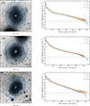 |
Fig. 8. Left: IE cutouts of the three galaxies of interest, displayed using hybrid histogram equalisation and logarithmic scale. Ellipses of the AutoProf profiles are displayed in blue. Right: Corresponding surface brightness profiles (solid lines) and their uncertainties (semi-transparent areas). The limiting surface brightness for extended emission on a 10″ × 10″ scale is taken from Cuillandre et al. (2025) and is shown as a dotted line for each band. |
Further out (beyond 600, 550, and 250 arcsec, respectively; or approximately 55, 50, and 20 kpc), the NGC 1549, NGC 1553, and NGC 1546 profiles drop sharply. The presence of this decline is confirmed by visual inspection and persists when the constant background value used by AutoProf is slightly varied. We extract from the surface brightness profiles the total magnitude and effective (or half-light) radius in each Euclid filter, for the three galaxies of interest. We report our results in Table 2 and Table 3.
AutoProf estimation of magnitudes of the main galaxies of the ERO Dorado FoV.
AutoProf estimation of effective (half-light) radii of the main galaxies of the ERO Dorado FoV in the different filters.
Table 2 shows similar NIR magnitudes for NGC 1549 and NGC 1553, indicating they have at first order comparable masses (since NIR bands are less sensitive to variations in the mass-to-light ratio caused by different stellar populations and ages; e.g. Bell & de Jong 2001). The magnitudes of NGC 1546 and IC 2058 confirm their significantly lower mass, but their difference in IE magnitude imply different star-formation histories (or might also be due to differences in dust attenuation).
4.1.2. Bright GC candidate number and distribution
The selection process described in Sect. 3.3.1 ends up with 790 bright GC candidates. Most of them are measured in both VIS and NISP images, and have associated colours. We divided this sample into two subsamples based on their IE − HE colour. Although we did not find a clear bimodality in the distribution of this colour for our GC candidates, the spread in the observed colours is larger than the measurement uncertainties and we expect the two halves of the distributions to contain different proportions of red and blue clusters as defined in the literature (e.g. Kundu & Whitmore 2001; Peng et al. 2006). Hereafter, the definition of red and blue GCs used is based on whether IE − HE is larger or smaller than the median value (0.68), which is not identical to the definitions used in those previous studies.
Table 4 presents the bright GC candidates counts for the three main galaxies. To cope with the overlap between NGC 1549 and NGC 1553 (see Figs. 2 and 9), we artificially separated their GC population at an isophote of 25.5 mag arcsec−2 in the IE band (roughly, 33 kpc or 370 arcsec for NGC 1549, 29.5 kpc or 330 arcsec for NGC 1553, and 13.5 kpc or 150 arcsec for NGC 1546). We count GCs within that isophote.
Number (non-corrected for completeness) of bright (IE ≤ 24) GC candidates for each galaxy.
To compare the numbers of expected bright GCs to those we find in Table 4, we used the method described in Euclid Collaboration: Voggel et al. (2025). This paper describes a code to predict the total number of GCs in a given galaxy using a Monte Carlo simulation based on the empirical trend with galaxy magnitude and uses the dispersion of GC specific frequency as a function of host stellar mass to estimate the range of expected GCs (see also details in Figs. 3 and 4 of that paper). We find that the mean predicted total number of GCs in NGC 1553, NGC 1549, and NGC 1546 are 475, 324, and 77, respectively, which is consistent with the total GC numbers estimated in Harris et al. (2013), apart from NGC 1546. Considering the magnitude limit IE = 24 we use in this study for GC detection, we find respectively 259, 178, and 42 GCs that should be brighter than that limit and be detectable. Comparing this number of detected GCs (Table 4) with the expected number of GCs from the prediction method, we find that we detected 50%, 90%, and 20% of all potential GCs brighter than our selection limit. The low detection fraction of GCs detected in NGC 1546 is likely due to much of its outskirts not being covered by the Euclid FoV, and the choice of the IE = 25.5 isophote as search radius. The 90 % of recovered GCs for NGC 1549 is probably unrealistically high and likely means that the total GC system size prediction is underestimated for this case, and this galaxy hosts an above average number of GCs. The true efficiency of our selection method is likely somewhere between the 50 % of NGC 1553 and the 90 % fraction of NGC 1549.
The spatial distribution of the bright GC candidates across the FoV is presented through the density maps in Fig. 9. Blue GCs seem to be more uniformly distributed, which aligns with expectations if this GC component is accreted from (minor) mergers (Brodie & Strader 2006). Red GCs can form either through in situ processes (Forbes et al. 2018) or as a result of past mergers involving metal-rich satellites. Consequently, their higher concentration compared to bluer GCs aligns with expectations.
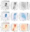 |
Fig. 9. Bright GC candidates density maps of the full ERO-D FoV (left column), with zooms on the NGC 1549-NGC 1553 pair (middle column), and on NGC 1546 (right column). The colour scale is the same for both zooms, where the density fields were re-evaluated locally using the samples within the cutouts. All GCs, blue GCs, and red GCs are represented in the upper, middle, and lower rows, respectively. Blue and red GCs are defined relative to the median IE − HE colour of the GC candidates, which is not indicative of an intrinsically bimodal population within our data. |
We also generated radial density profiles in Fig. 10. To determine the radius at which to stop the GC density estimation, we applied the same criterion detailed earlier. The three galaxies of interest show the expected trend: a high central concentration of GCs that decreases with increasing radius.
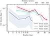 |
Fig. 10. GC density radial profiles for the three galaxies of interest. The shaded area around each curve represents the Poisson noise in the GC counts, computed for each bin. |
4.2. Properties of detected tidal features
4.2.1. Detection of tidal debris
In Fig. 11, we show that the original image together their unsharp masking and ellipse fitting residuals versions present numerous tidal debris, demonstrating the Euclid space telescope’s ability to detect such structures. We identify and classify those structures with the Jafar annotation tool. We list these features, in addition to several dwarf galaxies of interest and internal substructures (like rings or spiral arms), as seen in the top left panel of Fig. 12. Tidal features have been detected around NGC 1549, NGC 1553, and NGC 1546, but not around IC 2058.
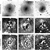 |
Fig. 11. IE surface brightness maps (top row), ellipse fitting residuals (middle row) and unsharp masked images (bottom row) for re-binned cutouts of the three galaxies of interest. The surface brightness image is in grayscale, black indicating where the surface brightness is below 21 mag arcsec−2, and white where it exceeds 27.5 mag arcsec−2. The unsharp masked image is produced using a 40 pixel standard deviation width Gaussian kernel. The scale and orientation of the cutouts are identical to those given in Fig. 8. In each figure, North is up, east is to the left. |
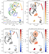 |
Fig. 12. Upper left: Features detected for each galaxy with the help of the IE images and residuals. Upper right: IE surface brightness map of the features. Those for which IE photometry can be performed are coloured according to their surface brightness and labelled. Their photometry is given in Table 5. They are discussed in the context of each galaxy they belong to in Sect. 4.2. Questions relative to their classification and nature are addressed in Sect. 5.1. Those for which this study is not possible are delineated in black. Especially, the photometry of the shells, of the uncertain features between NGC 1549 and NGC 1553, and of the features close to the galactic centres is not estimated. Lower left: IE − JE integrated fluxes colour map. The features with uncertain detection in the NIR bands appear in grey. Lower right: IE − JE GCs colour map. The average colours are weighted based on the uncertainties of the magnitudes that contribute to them. The features that encompass less than three bright GC candidates appear in grey. Surface brightness and colours are given respectively in mag arcsec−2 and in mag. |
Among those features, on the top-right panel of Fig. 12, we label with numbers those for which individual photometry was possible, at least in the IE band where they have been detected. The unlabelled structures are either too close to the galactic centre or they are located in the overlapping regions between NGC 1549 and NGC 1553; alternatively, they could be shells for which obtaining the necessary photometry is challenging (e.g. Sola et al. 2022). Some of the labelled features were poorly detected in NIR bands. In particular, the YE band seems to be the most affected by contaminants specific to the NIR bands, as discussed in Sect. 5. Therefore, we did not consider this filter for the individual feature photometry. We also excluded from the colour study those structures that are difficult to detect in the NIR bands. For the latter structures, the noise created by NIR-specific contaminants (including persistence) results in uncertainties ranging from over 0.2 up to several mag arcsec−2 in those bands (against below 0.1 mag arcsec−2 in the same bands for the structures we retained in the colour study).
Results from the photometry of the individual features are shown in the top right and bottom left panels of Fig. 12. We also calculate the median colour of the GC candidates each feature encompasses (bottom right panel of Fig. 12). Figure 13 presents a colour-colour diagram of the detected features, with the median colours of the associated GCs overplotted. We can see on this diagram that all the feature colours fall on or near the red-end regions of the stellar population models, excluding the youngest stellar populations (≈0.1–1 Gyr).
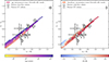 |
Fig. 13. Colour-colour plot of the ERO Dorado features, for both total flux photometry (square labels) and GCs photometry (round labels). The colours are given in magnitude. The interpolated metallicities and ages are obtained using the PEGASE (Le Borgne et al. 2004) single stellar population (SSP) model. However, the colour-coded area is consistent in age and metallicity across all the other SSP models tested. The feature labels are taken from Fig. 12. Their magnitude and colours are available in Table 5. |
When comparing the GC distribution in Fig. 9, we can observe location differences between the peaks of GC density and the ellipse profile centre of the galaxies. While the offset seen on NGC 1546 could be due to low-number statistics (see also the low GC count of this galaxy in Table 4), the offsets found for NGC 1549 and NGC 1553 seem real. Indeed, the scale of those offsets (over  ) is much larger than the central region where the galaxy is so bright that it makes detecting GCs impossible (under
  ).
).
It is worth mentioning that different offsets are seen in the blue and red GC distribution. If we approximate the total GC distribution around each galaxy by a Gaussian of standard deviation σ, the offsets vary over 3σ in the red and blue GC sub-samples, which suggests that these variations are significant. Finally, we did not find a systematic overdensity of GCs at the location of the debris and we speculate about possible reasons below.
-
Due to the presence of contaminants, we were compelled to restrict our sample of GC candidates to only the brightest ones (IE ≤ 24). The clustering of GCs in the vicinity of tidal features may remain undetected without including lower luminosity GCs. Higher resolution and deeper data could help overcome this limitation.
-
The detected tidal features could be formed from the material of small progenitors, such as dwarf galaxies, which do not necessarily contain GCs.
-
Phase-mixing of the GCs associated with tidal features may have erased any evidence of clustering, indicating that the mergers we observe traces of are not very recent.
-
If we consider the tidal features as remnants of the former disks of LTG progenitors that formed the galaxies observed in this study, we could hypothesise that there were few or no in situ GCs within these disks. Thus, we predominantly observe ex situ GCs here. They remain gravitationally bound to their host galaxy’s potential even during interactions with other galaxies, leaving the GC distribution unaffected and preventing any clustering from occurring.
-
For the galaxies involved in a merger, the GCs are not originally predominantly located in a disk but, rather, distributed in a halo. Consequently, they do not end up along the tidal features coming from the elongation of the former spiral arms.
4.2.2. NGC 1549
In Fig. 14, we see that the colour profile of NGC 1549 is flat, and is flatter than NGC 1553 in IE − JE. This is also visible with the help of the colour maps in Fig. 15. An interpretation of this is discussed in Sect. 5.1.
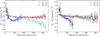 |
Fig. 14. Colour profiles for NGC 1549, NGC 1553, and NGC 1546. Left: IE − JE. Right: YE − HE. Such plots allow for the analysis of the differences between the galaxy profiles. In particular, the profile of NGC 1549 is the flattest, while that of NGC 1546 is the steepest across all colours. |
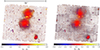 |
Fig. 15. Colour maps derived from ERO Dorado images. Left: IE − JE. Right: YE − HE. Such images allow for the qualitative analysis of colour differences between diffuse structures, as well as between central galactic regions and the stellar halo. In those figures, north is up, east is to the left. |
The unsharp masked image of NGC 1549 (Fig. 16) shows an internal substructure similar to diffuse spiral arms, with no visible star-formation region. The origin of this feature is uncertain. It could be the remnant of ancient galactic disk and bar, whose dynamics has been modified by a merger. This explanation would be consistent with UV data and traces of possible ancient star formation described in the literature (Rampazzo et al. 2020, 2021, 2022; see also Sect. 1).
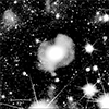 |
Fig. 16. IE unsharp masked image of the NGC 1549 centre, unveiling a bar and/or “pseudo-spiral arms”. In this figure, north is up, east is to the left. |
A large tidal feature (6) is visible to the north, and an umbrella-shaped structure composed of another tidal feature (1) and a shell is visible to the west. (6) is one of the bluest features detected, and (1) is one of the reddest. The NGC 1549 ellipse profile presents a slight bump from 13.38 kpc to 44.60 kpc (from 150 to 500 arcsec) from the galactic centre. This coincides with the position and extent of the tidal features (1) and (6). Their GCs photometry shows that these features might host red GCs. Finally, NGC 1549 also features a system of shells.
In the southern part of this galaxy in the direction of NGC 1553, three tidal features are visible, notably on the images of unsharp masking and ellipse fitting residuals, but remain very uncertain. We did not label them, but we note that one of them could be the southern extension of the northern large tidal feature (6).
4.2.3. NGC 1553
The colour profile trend of NGC 1553 (see Fig. 14) varies slightly with the choice of the photometric band. A blueward slope is observed with increasing radius for colours involving the IE band. For other colours, the profile is flatter, without excluding a slope if we consider its uncertainties.
This galaxy has the second highest peak density of GCs (see Fig. 9, Table 4). The distribution of GCs appears unusual. In its central region, the eastern side seems dominated by red GCs, while the western side is primarily populated by blue GCs. This asymmetry could be attributed to several factors, detailed below.
-
The effect could be real and due to a specific merger history, such as the accretion of a more metal-poor population along a preferred direction.
-
Depending on the galaxy orientation, there may be more galactic material along the line of sight between the observer and the GCs on one side of the galaxy compared to the other, causing varying levels of extinction across the two sides.
-
It could also be a combination of low-number statistics effects, typical central concentration of red GCs in the host galaxy, and the fact that blue GCs tend to have a shallower distribution around the host galaxy.
Figure 17 shows the NGC 1553 core, featuring dust lanes, a bar and diffuse spiral arms without star formation. Internal regions of this galaxy have a ring system. The most internal ring is spiral shaped and is particularly enlightened in unsharp masked images, as depicted in Fig. 17. The NGC 1553 ellipse profile presents a bump around 40″ from the galactic centre, probably caused by this ring/spiral structure.
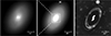 |
Fig. 17. IE image zooms on the central part of NGC 1553. In the left panel zoom, a dust lane is visible. Centre: Another zoom without any additional processing. Right: Unsharp masked corresponding image (using a 10 pixel standard deviation width Gaussian kernel) showing a ring feature composed of different arms and the spiral arms of the very central part. In this figure, North is up, east is to the left. |
Further from the centre, two ‘lobe’ features and a possible small tidal feature are observed, especially in the surface brightness and unsharp masked images (second row, and the first and third lines of Fig. 11). A second bump, around 100″, is very small but more prominent in the YE band, and seems to be caused by those features. Moreover, a system of shells is detected. Finally, the halo is distorted toward the northeast and southwest, yet without forming any elongated tidal structures. We have classified those distortions as the plumes (4) and (8). The feature (8) appears to be the faintest feature of this set.
4.2.4. NGC 1546
This is the first time that the tidal feature system of NGC 1546 is described in detail. The inspection of the image reveals the singular, if not unique morphology of NGC 1546. While Fig. 2 shows, in its outer regions, an extended and disturbed halo reminiscent of an elliptical galaxy, we see in Fig. 18 that in its outer regions, an entirely unperturbed flocculent disk galaxy.
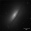 |
Fig. 18. IE image of the disk and dust lanes of NGC 1546, revealing its floculent nature. In this figure, north is up, east is to the left. |
Photometry of individual features.
NGC 1546 inner features are lobes and a small tidal feature. Further out, there is a shell system and a blue tidal feature (5). As previously mentioned, the blue GCs dominating this structure provoke an overdensity in the distribution (see Fig. 9). This can be the reason why the GC density profile of this galaxy rises significantly at large radii, as seen in Fig. 10. However, this behaviour could also result from the low-number statistics and therefore high uncertainties on this profile. GCs might be missing in the inner galaxy regions because of poor detection in this dusty environment. They could be, for instance, hidden or reddened by the dust and fall below our detection threshold or colour criteria. In the Sect. 5.1, we will discuss how the NGC 1546 morphology and GCs still strongly constrain its history of galactic mergers.
In the NGC 1546 ellipse profile, the innermost 40 arcsec are difficult to interpret due to the presence of arms and strong dust lanes in the disk, making the ellipse profile barely estimable. The tidal tail (5) and the shells are responsible for the bumps located from 150″ to 500″ from the centre.
4.2.5. Dwarf galaxies of interest and isolated features
In addition to the structures clearly associated with the studied galaxies, we note the presence of several features which are isolated or seem linked to some dwarf galaxies. This work presents the first mention of the following isolated features, demonstrating once again Euclid’s contribution to the detection of diffuse structures.
The tidal feature (2) of NGC 1549, which is not mentioned in the literature, is located to the east of the galaxy’s centre. It appears to be connected to the dwarf elliptical LSB galaxy (a) or [CMI2001] 5012-01 in Carrasco et al. (2001). Located at  ,
,  , this object is presented in the right panel of Fig. 19. The stream (2) could be composed of material from the dwarf galaxy (a), which would therefore be undergoing tidal disruption by its host galaxy, NGC 1549. However, the stream (2) exhibits colours that are not compatible within its uncertainties with those of the dwarf galaxy (labelled ‘a’ in Fig. 13 and Table 5). Therefore, this stream has a different metallicity than the dwarf (a), which seems to rule out the possibility of a link between them. Another hypothesis arises when considering the rather red colour of the dwarf galaxy (a) and the similarity of its GC colours to those of its host galaxy, NGC 1549 (seethe bottom-right panel of Fig. 12). This could suggest that the dwarf galaxy (a) is not composed of low-metallicity material, but rather of material from a massive progenitor. This would make the dwarf galaxy (a) a tidal dwarf located at 16.43 kpc from the centre of NGC 1549.
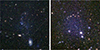 |
Fig. 19. Colour (IE, YE, HE) images of two objects of interest. As they overlap with the galaxies with which they are associated, obtaining these images required new cutouts (13.38 kpc × 13.38 kpc or 150″ × 150″), the use of MTObjects to mask sources, and the use of the GALFIT software (Peng et al. 2002) to determine and correct a tilted plane background. Finally, the colour image has been obtained with the Aladin software. Left: External star-forming region (possibly belonging to a satellite dwarf irregular galaxy) at the north of NGC 1553, labelled as (b) in Fig. 12. Right: Faint dwarf satellite galaxy at the north-west of NGC 1549, labelled as (a) in Fig. 12. In this figure, north is up, east is to the left. |
Around NGC 1553, we detect a clumpy object (b) at  ,
,  (see left panel of Fig. 19). Already mentioned in the catalogue of Carrasco et al. (2001) as a blue LSB dwarf, this object was previously discussed in Rampazzo et al. (2020), where its detection in UV with the Galaxy Evolution Explorer survey (GALEX) and the presence of H II regions were highlighted.
In the Euclid high-resolution image, its aspect and colour are consistent with a star-formation region. Moreover, Fig. 13 and Table 5 shows that the object (b) is compatible with low stellar ages and high metallicity. It could then be an outer star-forming region associated with NGC 1553, or even a tidal dwarf galaxy given its distance to the host centre. Another hypothesis could be that it is an external irregular star-forming dwarf galaxy though finding such an object as a galactic satellite is rare. Spectroscopic data could help to better identify and classify this object.
At a projected distance of approximately 60 kpc to the west of NGC 1549, we detect a faint tidal feature (7). Its progenitor might be the dwarf galaxy LEDA 75104 (Arp & Madore 1987), which is labelled as (d) Fig. 12.
Another faint tidal feature (3) is detected to the north of NGC 1546. A dwarf galaxy (labelled ‘c’, named SMDG J0415044−555618 and mentioned for the first time in Arp & Madore 1987) lies along its extension. However, the orientation of its semi-major axis, nearly perpendicular to the stream, challenges the hypothesis that it could be the progenitor of the tidal feature.
To the east of NGC 1546 and to the south of NGC 1553, one finds a feature (9) whose origin and nature are uncertain. Given its appearance as a detached tidal feature, we have classified this object as a ‘plume’. It could also be a tidally disrupting ultra-diffuse galaxy, similar to the case presented in Žemaitis et al. (2023). In the bottom-right panel of Fig. 12, we see that the GCs associated with this structure are red. This would be in favour of a tidal origin for this object, as it may have inherited its population of GCs from its progenitor. The flux photometry of this feature is limited by its non-detection in the NIR bands, likely due to contamination sources specific to this wavelength range in the ERO data (a topic that will be discussed in Sect. 2.2). The GC photometry places the feature at the furthest position from the stellar population model in the colour-colour diagram (Fig. 13), suggesting a complex star-formation history (or a high metallicity not taken into account by our SSP model) for this structure or its progenitor. A more refined stellar population synthesis model, enhanced data processing, and follow-up observations would enable a more in-depth investigation into its nature.
5. Discussion
5.1. Unveiling the mass assembly history of NGC 1549, NGC 1553, and NGC 1546
We explore the origin of the tidal features around the three brightest galaxies analysed in previous sections. One prime driver is to determine whether they originate from ancient mergers or were more recently formed due to the on-going interactions of the massive galaxies in the ERO-D field.
The structures (1), (2), (3), and (7) are too thin for their progenitors to be dynamically hot massive objects, such as the ETGs discussed in this study. Even the larger structure (6) remains too thin to be a deformation of the NGC 1549 halo. Furthermore, its direction does not point clearly toward any galaxy of the Dorado group. This rules out the possibility that this tidal feature is caused by a current interaction with a massive galaxy. We therefore argue that the tidal features (1), (2), (3), (6), and (7) are likely stellar streams, whose progenitors are lower mass galaxies that have been accreted. On the other hand, structures (4), (5), and (8) have shapes and sizes compatible with a halo disturbance caused by an ongoing interaction. We therefore tentatively classify them as plumes and tidal tails.
Besides the shapes of the structures, further clues on their origin may be derived from their colour. Stellar population models show that Euclid photometric bands colours of stellar structures not affected by on-going star formation vary much more with metallicity than with age (Kluge et al. 2025; Saifollahi et al. 2025a; Hunt et al. 2025). Therefore, we make the assumption that the differences in colours between individual tidal features or in the profile of ETGs are primarily due to differences in metallicity.
The flat colour profile of NGC 1549 suggests a relatively homogeneous mix of metal-rich and metal-poor stellar populations, possibly caused by a major merger (e.g. Di Matteo et al. 2009; Kim & Im 2013; Suess et al. 2020) linked to the largest structure: the north tidal stream (6). Indeed, colour maps (Fig. 15) show that it is redder than the halo of NGC 1549. This argues for a massive progenitor, likely more metal-rich than the NGC 1549 external parts. Since this galaxy exhibits the highest numbers of GCs, the progenitor of the large stellar stream (6) could have brought its GCs into the body of NGC 1549.
The stream (1) belonging to an umbrella-shaped feature is red. We can infer that this metal-rich stellar material comes either from the galactic centre of NGC 1549 or from an external progenitor more massive than a dwarf galaxy.
Given the previous considerations on the nature of the tidal features, the only remaining possible tidal features linked to a possible ongoing interaction between NGC 1549 and NGC 1553 are their shells and the NGC 1553 plumes (4) and (8). However, (4) seems oriented towards NGC 1546, and would therefore be caused by the gravitational attraction of the latter galaxy rather than that of NGC 1553. As for the shells, simulations (e.g. Ebrova 2013; Pop et al. 2018) show that they could not have been produced by the mutual current interaction between NGC 1553 and NGC 1549, but rather by past radial mergers that occurred in both galaxies. A tracer of a potential on-going interaction between NGC 1549 and NGC 1553 is possibly the plume (8) and the symmetric offsets in GC distribution peaks for both galaxies. This clear lack of evidence of any interaction is expected for massive ETGs, whose structure tends to be stronger than the rotation-supported one of a less massive LTG. An ETG would consequently preferentially form plumes, or even produce no tidal feature, rather than elongated bridges or tidal tails (e.g. Duc & Renaud 2013).
NGC 1553 exhibits inner spiral arms as well as traces of possible current and ancient star-forming activity revealed by the multi-wavelength data (see Sect. 1 for references). This galaxy could be a former LTG whose star formation was quenched and that has recently transitioned to an ETG following a series of minor mergers, those that are responsible for the formation of the shells observed in its main body (e.g. Petersson et al. 2023; Rutherford et al. 2024). This is consistent with the colour gradient of NGC 1553 showing evidence of material with lower metallicity and thus bluer colour in its outer regions (e.g. La Barbera et al. 2011; Kennedy et al. 2016; Marian et al. 2018). This last observation is in favour of more recent mergers, since phase-mixing has not yet blended stellar populations of different metallicities. An alternative scenario proposes that NGC 1553 underwent a transformation into an ETG through mergers, resulting in the loss of its initial angular momentum, followed by the inward migration of material that formed an inner disk at its centre (e.g. Shapiro et al. 2010). This interpretation is supported by the presence of the bar in the centre of NGC 1553, which could have funnelled material inwards (e.g. Gadotti et al. 2015). In the first scenario, the galaxy would remain a fast rotator, but not in the second. Therefore, a kinematic analysis of the inner and outer stellar populations with integral field units could help distinguishing the two scenarios (e.g. Cappellari 2016).
Making a claim about a recent transition from LTG to ETG for NGC 1549 would be more speculative: aside from the structure at its centre resembling diffuse spiral arms or a bar and visible only with unsharp masking (Fig. 16), its morphology is that of a pure elliptical galaxy, and the literature (e.g. Rampazzo et al. 2020, 2021, 2022) reports evidence of past but not current star formation. However, the mergers responsible for the shells may still have contributed to the dissipative events that led to the cessation of this star formation. An ancient major merger associated to a violent relaxation and phase mixing of the stars would explain its flat colour profile.
NGC 1546 appears as a hybrid object, consisting of an inner flocculent star-forming disk and a prominent outer diffuse stellar halo. The latter appears perturbed, making a tidal tail (5) oriented towards NGC 1553. An interaction with this massive galaxy is thus the likely origin of this tidal feature. The absence of any form of disturbance in the inner young disk excludes the possibility of a recent major merger. Its diffuse stellar halo could have been assembled by multiple minor mergers, a scenario consistent with the presence of a population of blue GCs at its location. Nevertheless, objects like NGC 1546 remain intriguing in groups.
The edge-on spiral IC 2058, whose disc is of a similar size to that of NGC 1546, shows no detectable stellar halo in Euclid images. Surprisingly, no warp is observed either, despite its apparent proximity to the massive galaxy NGC 1553. This challenges the hypothesis that the galaxy is already physically bound to the group (e.g. Iovino 2002).
With this interpretation regarding the origin and nature of each tidal feature, we can return to the question of GC clustering for detecting such structures. We notice that GC distribution disturbances are only seen at the locations of suspected major interactions and mergers. Indeed, in the right-hand column of Fig. 9, we observe a blue GC overdensity at the location of tidal feature (5), which is interpreted to indicate an ongoing major interaction, and offsets are detected around NGC 1549 and NGC 1553, which are suspected to be in interaction. Thus, although our results indicate that in these Euclid images, studying GC clustering alone is not sufficient for detecting tidal features, we see that analysing the GC distribution is still valuable for identifying major interactions and mergers. To validate or refute this preliminary conclusion, GC clustering should be analysed on a statistical sample of galaxies with observable debris. Such a study will be made possible by the EWS data.
5.2. Prospects for LSB detection in the EWS
Due to the contaminants described earlier, the gain of Euclid in terms of surface brightness limit is not obvious when comparing the ERO-D fields and DECaLS fields. However, the DECaLS image also suffers from contamination sources, such as CCD gaps, halos from bright stars, larger PSF, and higher sky background. This can lead to false positives in the search for tidal features, as seen in the example of Fig. 20. Since the two instruments are not affected by the same systematic effects, a suspected tidal feature in the DECaLS image can be confirmed or rejected in the Euclid image and vice versa, enabling extremely robust diffuse structure detection. Euclid’s optics are key in this study, as its sharp PSF does not spread Milky Way star light over large radial distances. Moreover, the superior resolution of Euclid images makes them better suited for determining the nature of the detected tidal features, and in particular the smallest ones (the PSF FWHM is  for Euclid IE as explained in Cuillandre et al. 2025, and
  for DECaLS i). The DESI Legacy survey, which covers a large portion of the EWS, could serve as a complement to the first Euclid data releases for a statistical study of tidal features. For the southern hemisphere, they will eventually be replaced by the Legacy Survey of Space and Time (LSST) data from the Vera Rubin Observatory.
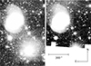 |
Fig. 20. Left: Example of possible false positive in diffuse structure detection with the DECaLS image. The light from a Milky Way star halo seems to form a tidal feature at the south of NGC 1546. Right: Same cutout for the Euclid IE image. |
The average surface brightness of the faintest feature detected in ERO-D (that is to say 28.00 ± 0.01 mag arcsec−2 in IE for the plume 8) does not reflect the intrinsic detection capabilities of Euclid, but rather specific limitations of the ERO-D data. Indeed, we do not detect the features that are fainter than the stray light. This result is still highly promising, as even with the inherent limitations of the ERO-D data set, Euclid reaches performance comparable to the one of the deepest surveys currently available. Additionally, Euclid also observes in the NIR, a wavelength range where the LSB realm remains unexplored.
Finally, it is worth noticing that the ERO pipeline used for ERO-D data processing is different from the EWS pipeline. Indeed, the ERO pipeline is optimised for LSB signal preservation on extended objects (even when filling most of the Euclid FoV, Cuillandre et al. 2025), whereas the EWS pipeline aims at producing excellent photometry of distant, and therefore small, sources. The methods used, particularly for background subtraction, could therefore vary from the ERO to the EWS pipelines, and the same applies to performance in terms of LSB signal preservation. Comparisons of EWS images to data from ground-based facilities could thus end up showing differences. A systematic study of the effect of the EWS pipeline on LSB objects is necessary for more accurate predictions of tidal features detection limits.
6. Summary and conclusions
The Euclid space telescope provides us with a groundbreaking view of four Dorado group galaxies, NGC 1549, NGC 1553, NGC 1546, and IC 2058. This image reveals an exceptional environment, rich in past collisions, and potential ongoing interactions. ERO-D allows us to map out an unprecedentedly exhaustive description of their tidal debris systems. The detection of the morphological structures and GCs of these galaxies summarised in Fig. 21 alongside their photometry led to a series of conclusions regarding the mass assembly history of the compact group SCG 0414−5559 formed by these galaxies.
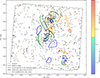 |
Fig. 21. Distribution of the bright GC candidates in the ERO-D field. Each dot is a GC candidate and its colour is scaled according to its IE − HE colour. Outlines of tidal and internal stellar features have been overlaid on the plot. |
-
NGC 1549 is an elliptical galaxy surrounded by a wealth of tidal features best explained by a past major merger event. This hypothesis is consistent with the flat colour profile of its stellar halo. An LSB dwarf galaxy is observed in its direction. However, its association with a nearby detected stream appears unlikely due to their difference in colours.
-
NGC 1553 has a star-forming structure and spiral arms in the centre and innermost ring. It has probably recently transitioned to the ETG regime due to radial minor mergers, as evidenced by the surrounding shells.
-
NGC 1546 is a rare specimen of a non-perturbed star-forming disk galaxy with a large disturbed halo. The colour of its tidal tail and its GCs suggest that this halo has been fed by dwarf accretions, then distorted probably due to tidal forces caused by NGC 1553.
-
IC 2058 is a pure disk galaxy which does not exhibit any tidal features or other morphological signs of membership to this compact group.
-
The ERO-D data also revealed more isolated features: two stellar streams and a structure that could be the bright end of a larger tidal feature from NGC 1553 or a tidally disrupted ultra-diffuse galaxy.
The ERO-D data were acquired from a single ROS, as will be the case for each stack in the EWS. Hence, this work can be considered as a pathfinder for the EWS researches on diffuse features for galactic merger history studies. We have thus drawn several conclusions regarding the detection in the ERO-D data set and prospects for the EWS, presented below.
-
Several sources of contamination have been identified. In particular, stray light has an impact on the detection of extended and faint stellar structures in the IE band, while persistence in the NISP detectors introduces additional uncertainties in the photometry of their counterparts in the NIR regime.
-
In the ERO-D image, we have been able to detect tidal features, reaching IE ≈ 28 mag arcsec−2. This is comparable to the deepest ground-based wide surveys (e.g. DESI Legacy and the future LSST), which will complement Euclid data but are affected by different systematic effects. Provided that the aforementioned data limitations are managed and the LSB signal is preserved along the EWS image processing pipeline, EWS data are poised to detect fainter features with better photometry.
-
The GCs detected by Euclid, their distribution, and their colour within each feature provide additional information that is useful for interpreting the nature of the structures and their progenitors. However, GC clustering alone does not enable the detection of tidal features in a systematic way. Exceptions can be found in cases involving major mergers, with a GC overdensity detected in the same location as a tidal tail, along with GC distribution peak offsets for two galaxies involved in a possible interaction.
With images matching the sensitivity of the deepest wide surveys currently available and providing superior resolution, Euclid enables detailed characterisations of tidal features in Local Universe galaxies (including the smallest structures) and studies of their GC populations. The EWS will allow for those studies to be extended to statistical samples on the visible and NIR extragalactic sky.
Acknowledgments
The authors are grateful to the anonymous referee for their constructive feedback, which significantly improved the manuscript. The Euclid Consortium acknowledges the European Space Agency and a number of agencies and institutes that have supported the development of Euclid, in particular the Agenzia Spaziale Italiana, the Austrian Forschungsförderungsgesellschaft funded through BMK, the Belgian Science Policy, the Canadian Euclid Consortium, the Deutsches Zentrum für Luft- und Raumfahrt, the DTU Space and the Niels Bohr Institute in Denmark, the French Centre National d’Etudes Spatiales, the Fundação para a Ciência e a Tecnologia, the Hungarian Academy of Sciences, the Ministerio de Ciencia, Innovación y Universidades, the National Aeronautics and Space Administration, the National Astronomical Observatory of Japan, the Netherlandse Onderzoekschool Voor Astronomie, the Norwegian Space Agency, the Research Council of Finland, the Romanian Space Agency, the State Secretariat for Education, Research, and Innovation (SERI) at the Swiss Space Office (SSO), and the United Kingdom Space Agency. A complete and detailed list is available on the Euclid web site (https://www.euclid-ec.org). This work has made use of the Early Release Observations (ERO) data from the Euclid mission of the European Space Agency (ESA), 2024, https://doi.org/10.57780/esa-qmocze3 Euclid Early Release Observations (2024). This research has made use of the SIMBAD database (Wenger et al. 2000), operated at CDS, Strasbourg, France, the VizieR catalogue access tool (Ochsenbein et al. 2000), CDS, Strasbourg, France (DOI : 10.26093/cds/vizier), and the Aladin sky atlas (Bonnarel et al. 2000; Boch & Fernique 2014) developed at CDS, Strasbourg Observatory, France and SAOImageDS9 (Joye & Mandel 2003). This work has been done using the following software, packages and PYTHON libraries: NUMPY (van der Walt et al. 2011), SCIPY (Virtanen et al. 2020), ASTROPY (Astropy Collaboration 2018), SCIKIT-LEARN (Pedregosa et al. 2011). The authors are grateful for financial support under the grant WIDERA ExGal-Twin, GA 101158446. E. Sola is grateful to the Leverhulme Trust for funding under the grant number RPG-2021-205. O. Müller is grateful to the Swiss National Science Foundation for financial support under the grant number PZ00P2_202104. This research was supported by the International Space Science Institute (ISSI) in Bern, through ISSI International Team project #534. This research makes use of ESA Datalabs (Navarro et al. 2024, datalabs.esa.int), an initiative by ESA’s Data Science and Archives Division in the Science and Operations Department, Directorate of Science.
References
- Abraham, R. G., & van Dokkum, P. G. 2014, PASP, 126, 55 [Google Scholar]
- Aihara, H., Arimoto, N., Armstrong, R., et al. 2017, PASJ, 70, S4 [NASA ADS] [Google Scholar]
- Akhlaghi, M., & Ichikawa, T. 2015, ApJS, 220, 1 [Google Scholar]
- Annibali, F., Beccari, G., Bellazzini, M., et al. 2020, MNRAS, 491, 5101 [NASA ADS] [Google Scholar]
- Arp, H. 1966, ApJS, 14, 1 [NASA ADS] [CrossRef] [Google Scholar]
- Arp, H. C., & Madore, B. 1987, A Catalogue of Southern Peculiar Galaxies and Associations (Cambridge: Cambridge University Press) [Google Scholar]
- Astropy Collaboration (Robitaille, T. P., et al.) 2013, A&A, 558, A33 [NASA ADS] [CrossRef] [EDP Sciences] [Google Scholar]
- Astropy Collaboration (Price-Whelan, A. M., et al.) 2018, AJ, 156, 123 [Google Scholar]
- Astropy Collaboration (Price-Whelan, A. M., et al.) 2022, ApJ, 935, 167 [NASA ADS] [CrossRef] [Google Scholar]
- Barbary, K. 2016, J. Open Source Softw., 1, 58 [Google Scholar]
- Barnes, J. E. 2004, MNRAS, 350, 798 [NASA ADS] [CrossRef] [Google Scholar]
- Bell, E. F., & de Jong, R. S. 2001, ApJ, 550, 212 [Google Scholar]
- Belokurov, V., Zucker, D. B., Evans, N. W., et al. 2006, ApJ, 642, L137 [Google Scholar]
- Bertin, E., & Arnouts, S. 1996, A&AS, 117, 393 [NASA ADS] [CrossRef] [EDP Sciences] [Google Scholar]
- Bi, S., Feng, H., & Ho, L. C. 2020, ApJ, 900, 124 [NASA ADS] [CrossRef] [Google Scholar]
- Bílek, M., Duc, P.-A., Cuillandre, J.-C., et al. 2020, MNRAS, 498, 2138 [Google Scholar]
- Blakeslee, J. P., Lucey, J. R., Barris, B. J., Hudson, M. J., & Tonry, J. L. 2001, MNRAS, 327, 1004 [NASA ADS] [CrossRef] [Google Scholar]
- Blumenthal, K. A., & Barnes, J. E. 2018, MNRAS, 479, 3952 [Google Scholar]
- Boch, T., & Fernique, P. 2014, in Astronomical Data Analysis Software and Systems XXIII, eds. N. Manset, & P. Forshay, ASP Conf. Ser., 485, 277 [NASA ADS] [Google Scholar]
- Bonnarel, F., Fernique, P., Bienaymé, O., et al. 2000, A&AS, 143, 33 [NASA ADS] [CrossRef] [EDP Sciences] [Google Scholar]
- Borlaff, A., Eliche-Moral, M. C., Rodríguez-Pérez, C., et al. 2014, A&A, 570, A103 [NASA ADS] [CrossRef] [EDP Sciences] [Google Scholar]
- Borlaff, A., Trujillo, I., Román, J., et al. 2019, A&A, 621, A133 [NASA ADS] [CrossRef] [EDP Sciences] [Google Scholar]
- Bradley, L., Sipocz, B., Robitaille, T., et al. 2016, Astrophysics Source Code Library [record ascl:1609.011] [Google Scholar]
- Bridges, T. J., & Hanes, D. A. 1990, AJ, 99, 1100 [Google Scholar]
- Brodie, J. P., & Strader, J. 2006, ARA&A, 44, 193 [Google Scholar]
- Brough, S., Collins, C., Demarco, R., et al. 2020, ArXiv e-prints [arXiv:2001.11067] [Google Scholar]
- Bullock, J. S., & Johnston, K. V. 2005, ApJ, 635, 931 [Google Scholar]
- Capaccioli, M., Spavone, M., Grado, A., et al. 2015, A&A, 581, A10 [NASA ADS] [CrossRef] [EDP Sciences] [Google Scholar]
- Cappellari, M. 2016, ARA&A, 54, 597 [Google Scholar]
- Carlsten, S. G., Greene, J. E., Beaton, R. L., Danieli, S., & Greco, J. P. 2022, ApJ, 933, 47 [CrossRef] [Google Scholar]
- Carrasco, E. R., Mendes de Oliveira, C., Infante, L., & Bolte, M. 2001, AJ, 121, 148 [NASA ADS] [CrossRef] [Google Scholar]
- Coccato, L., Gerhard, O., Arnaboldi, M., et al. 2009, MNRAS, 394, 1249 [Google Scholar]
- Cohen, J. G. 2000, AJ, 119, 162 [Google Scholar]
- Comerón, S., Salo, H., Laurikainen, E., et al. 2014, A&A, 562, A121 [Google Scholar]
- Conselice, C. J. 2014, ARA&A, 52, 291 [CrossRef] [Google Scholar]
- Cropper, M., Pottinger, S., Azzollini, R., et al. 2018, in Space Telescopes and Instrumentation 2018: Optical, Infrared, and Millimeter Wave, eds. M. Lystrup, H. A. MacEwen, G. G. Fazio, et al., SPIE Conf. Ser., 10698, 1069828 [Google Scholar]
- Cuillandre, J. C., Bertin, E., Bolzonella, M., et al. 2025, A&A, 697, A6 [Google Scholar]
- de Vaucouleurs, G., de Vaucouleurs, A., Corwin, H. G., Jr., et al. 1991, Third Reference Catalogue of Bright Galaxies (New York, NY, USA: Springer) [Google Scholar]
- Dekel, A., & Silk, J. 1986, ApJ, 303, 39 [Google Scholar]
- DES Collaboration (Abbott, T. M. C.) 2021, ApJS, 255, 20 [NASA ADS] [CrossRef] [Google Scholar]
- Dey, A., Schlegel, D. J., Lang, D., et al. 2019, AJ, 157, 168 [Google Scholar]
- Di Matteo, P., Pipino, A., Lehnert, M. D., Combes, F., & Semelin, B. 2009, A&A, 499, 427 [NASA ADS] [CrossRef] [EDP Sciences] [Google Scholar]
- Duc, P.-A., & Renaud, F. 2013, in Lect. Notes Phys., eds. J. Souchay, S. Mathis, & T. Tokieda (Berlin: Springer Verlag), 861, 327 [NASA ADS] [CrossRef] [Google Scholar]
- Duc, P.-A., Cuillandre, J.-C., Karabal, E., et al. 2015, MNRAS, 446, 120 [Google Scholar]
- Dupraz, C., Combes, F., & Prieur, J. L. 1987, in Structure and Dynamics of Elliptical Galaxies, ed. P. T. de Zeeuw, 127, 469 [Google Scholar]
- Durrell, P. R., Mihos, J. C., Feldmeier, J. J., Jacoby, G. H., & Ciardullo, R. 2003, ApJ, 582, 170 [NASA ADS] [CrossRef] [Google Scholar]
- Ebrova, I. 2013, Ph.D. Thesis, Charles University in Prague, Czech Republic [Google Scholar]
- Ellison, S. L., Viswanathan, A., Patton, D. R., et al. 2019, MNRAS, 487, 2491 [NASA ADS] [CrossRef] [Google Scholar]
- Erwin, P., Pohlen, M., & Beckman, J. E. 2008, AJ, 135, 20 [Google Scholar]
- Euclid Collaboration (Borlaff, A. S., et al.) 2022, A&A, 657, A92 [NASA ADS] [CrossRef] [EDP Sciences] [Google Scholar]
- Euclid Collaboration (Scaramella, R., et al.) 2022, A&A, 662, A112 [NASA ADS] [CrossRef] [EDP Sciences] [Google Scholar]
- Euclid Collaboration (Schirmer, M., et al.) 2022, A&A, 662, A92 [NASA ADS] [CrossRef] [EDP Sciences] [Google Scholar]
- Euclid Collaboration (Jahnke, K., et al.) 2025, A&A, 697, A3 [Google Scholar]
- Euclid Collaboration (Cropper, M. S., et al.) 2025, A&A, 697, A2 [Google Scholar]
- Euclid Collaboration (Mellier, Y., et al.) 2025, A&A, 697, A1 [Google Scholar]
- Euclid Collaboration (Voggel, K., et al.) 2025, A&A, 693, A251 [Google Scholar]
- Euclid Early Release Observations. 2024, https://doi.org/10.57780/esa-qmocze3 [Google Scholar]
- Fernique, P., Boch, T., Donaldson, T., et al. 2014, MOC– HEALPix Multi-Order Coverage Map Version 1.0, IVOA Recommendation 02 June 2014 [Google Scholar]
- Ferrarese, L., Côté, P., Cuillandre, J.-C., et al. 2012, ApJS, 200, 4 [Google Scholar]
- Firth, P., Evstigneeva, E. A., Jones, J. B., et al. 2006, MNRAS, 372, 1856 [NASA ADS] [CrossRef] [Google Scholar]
- Forbes, D. A., Bastian, N., Gieles, M., et al. 2018, Proc. R. Soc. Lond. Ser. A, 474, 20170616 [Google Scholar]
- Foster, C., Lux, H., Romanowsky, A. J., et al. 2014, MNRAS, 442, 3544 [NASA ADS] [CrossRef] [Google Scholar]
- Freeman, K. C. 1975, in Dynamics of the Solar Systems, ed. A. Hayli, IAU Symp., 69, 367 [Google Scholar]
- Gadotti, D. A., Seidel, M. K., Sánchez-Blázquez, P., et al. 2015, A&A, 584, A90 [NASA ADS] [CrossRef] [EDP Sciences] [Google Scholar]
- Garcia, A. M. 1993, A&AS, 100, 47 [NASA ADS] [Google Scholar]
- Greco, J. P., Greene, J. E., Strauss, M. A., et al. 2018, ApJ, 857, 104 [NASA ADS] [CrossRef] [Google Scholar]
- Greggio, L., Rejkuba, M., Gonzalez, O. A., et al. 2014, A&A, 562, A73 [NASA ADS] [CrossRef] [EDP Sciences] [Google Scholar]
- Guzmán, R. 2024, EAS2024, 1990 [Google Scholar]
- Harris, W. E. 2001, in Saas-Fee Advanced Course 28: Star Clusters, eds. L. Labhardt, & B. Binggeli, 223 [Google Scholar]
- Harris, W. E., Harris, G. L. H., & Alessi, M. 2013, ApJ, 772, 82 [Google Scholar]
- Hartke, J., Arnaboldi, M., Gerhard, O., et al. 2022, A&A, 663, A12 [NASA ADS] [CrossRef] [EDP Sciences] [Google Scholar]
- Hopp, U., Bender, R., Grupp, F., et al. 2014, in Ground-based and Airborne Telescopes V, eds. L. M. Stepp, R. Gilmozzi, & H. J. Hall, SPIE Conf. Ser., 9145, 91452D [NASA ADS] [Google Scholar]
- Huchra, J. P., & Geller, M. J. 1982, ApJ, 257, 423 [NASA ADS] [CrossRef] [Google Scholar]
- Hughes, A. K., Sand, D. J., Seth, A., et al. 2021, ApJ, 914, 16 [NASA ADS] [CrossRef] [Google Scholar]
- Hunt, L. K., Annibali, F., Cuillandre, J. C., et al. 2025, A&A, 697, A9 [NASA ADS] [CrossRef] [EDP Sciences] [Google Scholar]
- Huxor, A. P., Mackey, A. D., Ferguson, A. M. N., et al. 2014, MNRAS, 442, 2165 [Google Scholar]
- Ibata, R. A., McConnachie, A., Cuillandre, J.-C., et al. 2017, ApJ, 848, 128 [Google Scholar]
- Ibata, R., Malhan, K., Martin, N., et al. 2021, ApJ, 914, 123 [NASA ADS] [CrossRef] [Google Scholar]
- Iovino, A. 2002, AJ, 124, 2471 [NASA ADS] [CrossRef] [Google Scholar]
- Ivezić, Ž., Kahn, S. M., Tyson, J. A., et al. 2019, ApJ, 873, 111 [Google Scholar]
- Javanmardi, B., Martinez-Delgado, D., Kroupa, P., et al. 2016, A&A, 588, A89 [NASA ADS] [CrossRef] [EDP Sciences] [Google Scholar]
- Jedrzejewski, R. I. 1987, MNRAS, 226, 747 [Google Scholar]
- Joye, W. A., & Mandel, E. 2003, in Astronomical Data Analysis Software and Systems XII, eds. H. E. Payne, R. I. Jedrzejewski, & R. N. Hook, ASP Conf. Ser., 295, 489 [NASA ADS] [Google Scholar]
- Karabal, E., Duc, P. A., Kuntschner, H., et al. 2017, A&A, 601, A86 [NASA ADS] [CrossRef] [EDP Sciences] [Google Scholar]
- Karachentsev, I. D., Riepe, P., Zilch, T., et al. 2015, Astrophys. Bull., 70, 379 [NASA ADS] [CrossRef] [Google Scholar]
- Kennedy, R., Bamford, S. P., Häußler, B., et al. 2016, A&A, 593, A84 [NASA ADS] [CrossRef] [EDP Sciences] [Google Scholar]
- Kilborn, V. A., Koribalski, B. S., Forbes, D. A., Barnes, D. G., & Musgrave, R. C. 2005, MNRAS, 356, 77 [CrossRef] [Google Scholar]
- Kim, D., & Im, M. 2013, ApJ, 766, 109 [Google Scholar]
- Kim, J.-H., Wise, J. H., & Abel, T. 2009, ApJ, 694, L123 [NASA ADS] [CrossRef] [Google Scholar]
- King, I. R. 1966, AJ, 71, 64 [Google Scholar]
- Kluge, M., Neureiter, B., Riffeser, A., et al. 2020, ApJS, 247, 43 [Google Scholar]
- Kluge, M., Hatch, N. A., Montes, M., et al. 2025, A&A, 697, A13 [NASA ADS] [CrossRef] [EDP Sciences] [Google Scholar]
- Klypin, A., Kravtsov, A. V., Valenzuela, O., & Prada, F. 1999, ApJ, 522, 82 [Google Scholar]
- Koch, A., Hanke, M., & Kacharov, N. 2018, A&A, 616, A74 [NASA ADS] [CrossRef] [EDP Sciences] [Google Scholar]
- Koekemoer, A., & Roman Deep Fields Working Group. 2023, Am. Astron. Soc. Meet. Abstr., 55, 101.02 [Google Scholar]
- Koss, M. J., Treister, E., Kakkad, D., et al. 2023, ApJ, 942, L24 [Google Scholar]
- Kourkchi, E., & Tully, R. B. 2017, ApJ, 843, 16 [NASA ADS] [CrossRef] [Google Scholar]
- Kundu, A., & Whitmore, B. C. 2001, AJ, 121, 2950 [NASA ADS] [CrossRef] [Google Scholar]
- La Barbera, F., Ferreras, I., de Carvalho, R. R., et al. 2011, ApJ, 740, L41 [Google Scholar]
- Lahén, N., Johansson, P. H., Rantala, A., Naab, T., & Frigo, M. 2018, MNRAS, 475, 3934 [Google Scholar]
- Lançon, A., Larsen, S., Voggel, K., et al. 2021, in SF2A-2021: Proceedings of the Annual Meeting of the French Society of Astronomy and Astrophysics, eds. A. Siebert, K. Baillié, E. Lagadec, et al., 447 [Google Scholar]
- Le Borgne, D., Rocca-Volmerange, B., Prugniel, P., et al. 2004, A&A, 425, 881 [CrossRef] [EDP Sciences] [Google Scholar]
- Lim, S., Peng, E. W., Duc, P.-A., et al. 2017, ApJ, 835, 123 [NASA ADS] [CrossRef] [Google Scholar]
- Mackey, A. D., Huxor, A. P., Ferguson, A. M. N., et al. 2010, ApJ, 717, L11 [NASA ADS] [CrossRef] [Google Scholar]
- Mackey, D., Lewis, G. F., Brewer, B. J., et al. 2019, Nature, 574, 69 [NASA ADS] [CrossRef] [Google Scholar]
- Makarov, D., & Karachentsev, I. 2011, MNRAS, 412, 2498 [NASA ADS] [CrossRef] [Google Scholar]
- Malin, D. F., & Carter, D. 1983, ApJ, 274, 534 [Google Scholar]
- Mancillas, B., Duc, P.-A., Combes, F., et al. 2019, A&A, 632, A122 [NASA ADS] [CrossRef] [EDP Sciences] [Google Scholar]
- Marian, V., Ziegler, B., Kuchner, U., & Verdugo, M. 2018, A&A, 617, A34 [NASA ADS] [CrossRef] [EDP Sciences] [Google Scholar]
- Marleau, F. R., Cuillandre, J. C., Cantiello, M., et al. 2025, A&A, 697, A12 [NASA ADS] [CrossRef] [EDP Sciences] [Google Scholar]
- Martin, N. F., Ibata, R. A., Starkenburg, E., et al. 2022, MNRAS, 516, 5331 [NASA ADS] [CrossRef] [Google Scholar]
- Martínez-Delgado, D., Gabany, R. J., Crawford, K., et al. 2010, AJ, 140, 962 [Google Scholar]
- Massari, D., Dalessandro, E., Erkal, D., et al. 2025, A&A, 697, A8 [Google Scholar]
- Meisner, A. M., & Finkbeiner, D. P. 2014, ApJ, 781, 5 [Google Scholar]
- Merritt, A., van Dokkum, P., & Abraham, R. 2014, ApJ, 787, L37 [NASA ADS] [CrossRef] [Google Scholar]
- Mihos, C., Dubinski, J., & Hernquist, L. 1995, Am. Astron. Soc. Meet. Abstr., 186, 39.09 [Google Scholar]
- Miró-Carretero, J., Martínez-Delgado, D., Farràs-Aloy, S., et al. 2023, A&A, 669, L13 [NASA ADS] [CrossRef] [EDP Sciences] [Google Scholar]
- Miville-Deschênes, M. A., Duc, P. A., Marleau, F., et al. 2016, A&A, 593, A4 [Google Scholar]
- Mondelin, M., Bournaud, F., Cuillandre, J.-C., et al. 2025, A&A, 699, A214 [NASA ADS] [CrossRef] [EDP Sciences] [Google Scholar]
- Montes, M., Annibali, F., Bellazzini, M., et al. 2023, ArXiv e-prints [arXiv:2306.09414] [Google Scholar]
- Moore, B., Ghigna, S., Governato, F., et al. 1999, ApJ, 524, L19 [Google Scholar]
- Morales, G., Martínez-Delgado, D., Grebel, E. K., et al. 2018, A&A, 614, A143 [NASA ADS] [CrossRef] [EDP Sciences] [Google Scholar]
- Mosenkov, A., Rich, R. M., Koch, A., et al. 2020, MNRAS, 494, 1751 [NASA ADS] [CrossRef] [Google Scholar]
- Mould, J. R., Huchra, J. P., Freedman, W. L., et al. 2000, ApJ, 529, 786 [Google Scholar]
- Müller, O., Rich, R. M., Román, J., et al. 2019, A&A, 624, L6 [Google Scholar]
- Nasonova, O. G., de Freitas Pacheco, J. A., & Karachentsev, I. D. 2011, VizieR Online Data Catalog: Hubble flow around Fornax cluster of galaxies (Nasonova+, 2011), VizieR On-line Data Catalog: J/A+A/532/A104. Originally published. In: 2011A&A..532A.104N [Google Scholar]
- Navarro, V., del Rio, S., Diego, M. A., et al. 2024, in ESA Datalabs: Digital Innovation in Space Science, ed. A. Cortesi, (Singapore: Springer Nature), 1 [Google Scholar]
- Ochsenbein, F., Bauer, P., & Marcout, J. 2000, A&AS, 143, 23 [NASA ADS] [CrossRef] [EDP Sciences] [Google Scholar]
- Paturel, G., Petit, C., Prugniel, P., et al. 2003, A&A, 412, 45 [NASA ADS] [CrossRef] [EDP Sciences] [Google Scholar]
- Paudel, S., Yoon, S.-J., Yoo, J., et al. 2023, ApJS, 265, 57 [NASA ADS] [CrossRef] [Google Scholar]
- Pedregosa, F., Varoquaux, G., Gramfort, A., et al. 2011, J. Mach. Learn. Res., 12, 2825 [Google Scholar]
- Peng, C. Y., Ho, L. C., Impey, C. D., & Rix, H.-W. 2002, AJ, 124, 266 [Google Scholar]
- Peng, E. W., Jordán, A., Côté, P., et al. 2006, ApJ, 639, 95 [Google Scholar]
- Peng, E. W., Ferguson, H. C., Goudfrooij, P., et al. 2011, ApJ, 730, 23 [Google Scholar]
- Petersson, J., Renaud, F., Agertz, O., Dekel, A., & Duc, P.-A. 2023, MNRAS, 518, 3261 [Google Scholar]
- Pohlen, M., & Trujillo, I. 2006, A&A, 454, 759 [NASA ADS] [CrossRef] [EDP Sciences] [Google Scholar]
- Pop, A.-R., Pillepich, A., Amorisco, N. C., & Hernquist, L. 2018, MNRAS, 480, 1715 [Google Scholar]
- Pota, V., Forbes, D. A., Romanowsky, A. J., et al. 2013, MNRAS, 428, 389 [NASA ADS] [CrossRef] [Google Scholar]
- Prieur, J. L. 1990, in Dynamics and Interactions of Galaxies, ed. R. Wielen, 72 [Google Scholar]
- Quinn, P. J. 1984, ApJ, 279, 596 [Google Scholar]
- Raj, M. A., Awad, P., Peletier, R. F., et al. 2024, A&A, 690, A92 [NASA ADS] [CrossRef] [EDP Sciences] [Google Scholar]
- Rampazzo, R., Panuzzo, P., Vega, O., et al. 2013, MNRAS, 432, 374 [NASA ADS] [CrossRef] [Google Scholar]
- Rampazzo, R., Ciroi, S., Mazzei, P., et al. 2020, A&A, 643, A176 [NASA ADS] [CrossRef] [EDP Sciences] [Google Scholar]
- Rampazzo, R., Mazzei, P., Marino, A., et al. 2021, J. Astrophys. Astron., 42, 31 [Google Scholar]
- Rampazzo, R., Mazzei, P., Marino, A., et al. 2022, A&A, 664, A192 [NASA ADS] [CrossRef] [EDP Sciences] [Google Scholar]
- Rejkuba, M. 2012, Ap&SS, 341, 195 [Google Scholar]
- Rejkuba, M., Harris, W. E., Greggio, L., Crnojević, D., & Harris, G. L. H. 2022, A&A, 657, A41 [NASA ADS] [CrossRef] [EDP Sciences] [Google Scholar]
- Renaud, F., Segovia Otero, Á., & Agertz, O. 2022, MNRAS, 516, 4922 [NASA ADS] [CrossRef] [Google Scholar]
- Ricci, T. V., Steiner, J. E., Menezes, R. B., Slodkowski Clerici, K., & da Silva, M. D. 2023, MNRAS, 522, 2207 [Google Scholar]
- Román, J., Trujillo, I., & Montes, M. 2020, A&A, 644, A42 [NASA ADS] [CrossRef] [EDP Sciences] [Google Scholar]
- Rutherford, T. H., van de Sande, J., Croom, S. M., et al. 2024, MNRAS, 529, 810 [NASA ADS] [CrossRef] [Google Scholar]
- Saifollahi, T., Voggel, K., Lançon, A., et al. 2025a, A&A, 697, A10 [NASA ADS] [CrossRef] [EDP Sciences] [Google Scholar]
- Saifollahi, T., Lançon, A., Cantiello, M., et al. 2025b, A&A, submitted [arXiv:2503.16367] [Google Scholar]
- Saitoh, T. R., Daisaka, H., Kokubo, E., et al. 2009, PASJ, 61, 481 [NASA ADS] [Google Scholar]
- Sanders, D. B., & Mirabel, I. F. 1996, ARA&A, 34, 749 [Google Scholar]
- Sandin, C. 2014, A&A, 567, A97 [NASA ADS] [CrossRef] [EDP Sciences] [Google Scholar]
- Schlafly, E. F., & Finkbeiner, D. P. 2011, ApJ, 737, 103 [Google Scholar]
- Schlegel, D. J., Finkbeiner, D. P., & Davis, M. 1998, ApJ, 500, 525 [Google Scholar]
- Shapiro, K. L., Falcón-Barroso, J., van de Ven, G., et al. 2010, MNRAS, 402, 2140 [NASA ADS] [CrossRef] [Google Scholar]
- She, R., Ho, L. C., & Feng, H. 2017, ApJ, 835, 223 [NASA ADS] [CrossRef] [Google Scholar]
- Sola, E., Duc, P.-A., Richards, F., et al. 2022, A&A, 662, A124 [NASA ADS] [CrossRef] [EDP Sciences] [Google Scholar]
- Somerville, R. S., & Davé, R. 2015, ARA&A, 53, 51 [Google Scholar]
- Stone, C. J., Arora, N., Courteau, S., & Cuillandre, J.-C. 2021, MNRAS, 508, 1870 [NASA ADS] [CrossRef] [Google Scholar]
- Suess, K. A., Kriek, M., Price, S. H., & Barro, G. 2020, ApJ, 899, L26 [Google Scholar]
- Teeninga, P., Moschini, U., Trager, S. C., & Wilkinson, M. H. 2015, International Symposium on Mathematical Morphology and Its Applications to Signal and Image Processing (Springer), 157 [Google Scholar]
- Teeninga, P., Moschini, U., Trager, S. C., & Wilkinson, M. H. 2016, Math. Morphol.– Theory Appl., 1, 100 [Google Scholar]
- Toomre, A., & Toomre, J. 1972, ApJ, 178, 623 [Google Scholar]
- Trujillo, I., D’Onofrio, M., Zaritsky, D., et al. 2021, A&A, 654, A40 [NASA ADS] [CrossRef] [EDP Sciences] [Google Scholar]
- Tully, R. B., & Fisher, J. R. 1988, Catalog of Nearby Galaxies (Cambridge: Cambridge University Press) [Google Scholar]
- Usher, C., Forbes, D. A., Brodie, J. P., et al. 2012, MNRAS, 426, 1475 [Google Scholar]
- van der Walt, S., Colbert, S. C., & Varoquaux, G. 2011, Comput. Sci. Eng., 13, 22 [Google Scholar]
- Veljanoski, J., Ferguson, A. M. N., Mackey, A. D., et al. 2013, ApJ, 768, L33 [NASA ADS] [CrossRef] [Google Scholar]
- Virtanen, P., Gommers, R., Oliphant, T. E., et al. 2020, Nat. Methods, 17, 261 [Google Scholar]
- Voggel, K., Hilker, M., & Richtler, T. 2016, A&A, 586, A102 [NASA ADS] [CrossRef] [EDP Sciences] [Google Scholar]
- Weil, M. L., & Hernquist, L. 1993, in The Globular Cluster-Galaxy Connection, eds. G. H. Smith, & J. P. Brodie, ASP Conf. Ser., 48, 629 [Google Scholar]
- Wenger, M., Ochsenbein, F., Egret, D., et al. 2000, A&AS, 143, 9 [NASA ADS] [CrossRef] [EDP Sciences] [Google Scholar]
- Wright, E. L., Eisenhardt, P. R. M., Mainzer, A. K., et al. 2010, AJ, 140, 1868 [Google Scholar]
- York, D. G., Adelman, J., Anderson, J. E. Jr., et al. 2000, AJ, 120, 1579 [Google Scholar]
- Younger, J. D., Cox, T. J., Seth, A. C., & Hernquist, L. 2007, ApJ, 670, 269 [NASA ADS] [CrossRef] [Google Scholar]
- Žemaitis, R., Ferguson, A. M. N., Okamoto, S., et al. 2023, MNRAS, 518, 2497 [Google Scholar]
- Zöller, R., Kluge, M., Staiger, B., & Bender, R. 2024, ApJS, 271, 52 [CrossRef] [Google Scholar]
All Tables
AutoProf estimation of effective (half-light) radii of the main galaxies of the ERO Dorado FoV in the different filters.
Number (non-corrected for completeness) of bright (IE ≤ 24) GC candidates for each galaxy.
All Figures
|
Fig. 1. DECaLS colour image of the Dorado group. The brightest members are labeled in the figure. The HEALPix Multi-Order Coverage map (Fernique et al. 2014) of the Euclid ERO-D FoV is added to the image as a red-transparent overlay. The coordinates are given in RA, Dec. |
| In the text | |
|
Fig. 2. Euclid surface brightness maps in the IE band with a scale in mag arcsec−2 indicated to the bottom. Colour images made by co-adding the IE, the YE, and the HE bands using Astropy (Astropy Collaboration 2013, 2018, 2022) are super-imposed in the inner regions of the main galaxies. Top: Whole FoV (≈56 arcmin2) of the ERO-D observations. Lower-left: 300″ × 300″ cutout around IC 2058 and the dwarf galaxy PGC 75125. Lower-right: 600″ × 600″ cutout around NGC 1546. In this figure, north is up, east is to the left. |
| In the text | |
|
Fig. 3. Impact of varying detector sensitivities and persistence on tidal feature detection in NIR bands. Top: IE image centred on a diffuse feature at the north of NGC 1546. Bottom: Same field in HE, where the feature is much less visible. |
| In the text | |
|
Fig. 4. View of the 12 μm photometric band of the WISE IR survey (reprocessed by Meisner & Finkbeiner 2014), allowing us to probe the presence of Galactic cirrus. The ERO-D FoV is displayed in semi-transparent red. The coordinates are given in RA, Dec. |
| In the text | |
|
Fig. 5. Large-scale diffuse light component correction for the IE image. Left: Original IE image. Centre: sep background map. The MTObjects masks are in black. Right: sep local background-subtracted output IE image. |
| In the text | |
|
Fig. 6. Residual image subtracting the DECaLS i-band surface brightness map from the EuclidIE surface brightness map. The scale gives the residual in mag arcsec−2. Left: Residual image using the original IE image. The extended dark area in the lower part of the image indicates the possible presence of stray light. Right: Residual image using the IE corrected surface brightness map. |
| In the text | |
|
Fig. 7. GC completeness of ERO-D as a function of IE, SIM, the magnitude of artificial GCs injected in the data. Note: at the distance of the Dorado galaxies, real GCs are expected to be distributed between IE = 21 and IE = 25. |
| In the text | |
|
Fig. 8. Left: IE cutouts of the three galaxies of interest, displayed using hybrid histogram equalisation and logarithmic scale. Ellipses of the AutoProf profiles are displayed in blue. Right: Corresponding surface brightness profiles (solid lines) and their uncertainties (semi-transparent areas). The limiting surface brightness for extended emission on a 10″ × 10″ scale is taken from Cuillandre et al. (2025) and is shown as a dotted line for each band. |
| In the text | |
|
Fig. 9. Bright GC candidates density maps of the full ERO-D FoV (left column), with zooms on the NGC 1549-NGC 1553 pair (middle column), and on NGC 1546 (right column). The colour scale is the same for both zooms, where the density fields were re-evaluated locally using the samples within the cutouts. All GCs, blue GCs, and red GCs are represented in the upper, middle, and lower rows, respectively. Blue and red GCs are defined relative to the median IE − HE colour of the GC candidates, which is not indicative of an intrinsically bimodal population within our data. |
| In the text | |
|
Fig. 10. GC density radial profiles for the three galaxies of interest. The shaded area around each curve represents the Poisson noise in the GC counts, computed for each bin. |
| In the text | |
|
Fig. 11. IE surface brightness maps (top row), ellipse fitting residuals (middle row) and unsharp masked images (bottom row) for re-binned cutouts of the three galaxies of interest. The surface brightness image is in grayscale, black indicating where the surface brightness is below 21 mag arcsec−2, and white where it exceeds 27.5 mag arcsec−2. The unsharp masked image is produced using a 40 pixel standard deviation width Gaussian kernel. The scale and orientation of the cutouts are identical to those given in Fig. 8. In each figure, North is up, east is to the left. |
| In the text | |
|
Fig. 12. Upper left: Features detected for each galaxy with the help of the IE images and residuals. Upper right: IE surface brightness map of the features. Those for which IE photometry can be performed are coloured according to their surface brightness and labelled. Their photometry is given in Table 5. They are discussed in the context of each galaxy they belong to in Sect. 4.2. Questions relative to their classification and nature are addressed in Sect. 5.1. Those for which this study is not possible are delineated in black. Especially, the photometry of the shells, of the uncertain features between NGC 1549 and NGC 1553, and of the features close to the galactic centres is not estimated. Lower left: IE − JE integrated fluxes colour map. The features with uncertain detection in the NIR bands appear in grey. Lower right: IE − JE GCs colour map. The average colours are weighted based on the uncertainties of the magnitudes that contribute to them. The features that encompass less than three bright GC candidates appear in grey. Surface brightness and colours are given respectively in mag arcsec−2 and in mag. |
| In the text | |
|
Fig. 13. Colour-colour plot of the ERO Dorado features, for both total flux photometry (square labels) and GCs photometry (round labels). The colours are given in magnitude. The interpolated metallicities and ages are obtained using the PEGASE (Le Borgne et al. 2004) single stellar population (SSP) model. However, the colour-coded area is consistent in age and metallicity across all the other SSP models tested. The feature labels are taken from Fig. 12. Their magnitude and colours are available in Table 5. |
| In the text | |
|
Fig. 14. Colour profiles for NGC 1549, NGC 1553, and NGC 1546. Left: IE − JE. Right: YE − HE. Such plots allow for the analysis of the differences between the galaxy profiles. In particular, the profile of NGC 1549 is the flattest, while that of NGC 1546 is the steepest across all colours. |
| In the text | |
|
Fig. 15. Colour maps derived from ERO Dorado images. Left: IE − JE. Right: YE − HE. Such images allow for the qualitative analysis of colour differences between diffuse structures, as well as between central galactic regions and the stellar halo. In those figures, north is up, east is to the left. |
| In the text | |
|
Fig. 16. IE unsharp masked image of the NGC 1549 centre, unveiling a bar and/or “pseudo-spiral arms”. In this figure, north is up, east is to the left. |
| In the text | |
|
Fig. 17. IE image zooms on the central part of NGC 1553. In the left panel zoom, a dust lane is visible. Centre: Another zoom without any additional processing. Right: Unsharp masked corresponding image (using a 10 pixel standard deviation width Gaussian kernel) showing a ring feature composed of different arms and the spiral arms of the very central part. In this figure, North is up, east is to the left. |
| In the text | |
|
Fig. 18. IE image of the disk and dust lanes of NGC 1546, revealing its floculent nature. In this figure, north is up, east is to the left. |
| In the text | |
|
Fig. 19. Colour (IE, YE, HE) images of two objects of interest. As they overlap with the galaxies with which they are associated, obtaining these images required new cutouts (13.38 kpc × 13.38 kpc or 150″ × 150″), the use of MTObjects to mask sources, and the use of the GALFIT software (Peng et al. 2002) to determine and correct a tilted plane background. Finally, the colour image has been obtained with the Aladin software. Left: External star-forming region (possibly belonging to a satellite dwarf irregular galaxy) at the north of NGC 1553, labelled as (b) in Fig. 12. Right: Faint dwarf satellite galaxy at the north-west of NGC 1549, labelled as (a) in Fig. 12. In this figure, north is up, east is to the left. |
| In the text | |
|
Fig. 20. Left: Example of possible false positive in diffuse structure detection with the DECaLS image. The light from a Milky Way star halo seems to form a tidal feature at the south of NGC 1546. Right: Same cutout for the Euclid IE image. |
| In the text | |
|
Fig. 21. Distribution of the bright GC candidates in the ERO-D field. Each dot is a GC candidate and its colour is scaled according to its IE − HE colour. Outlines of tidal and internal stellar features have been overlaid on the plot. |
| In the text | |
Current usage metrics show cumulative count of Article Views (full-text article views including HTML views, PDF and ePub downloads, according to the available data) and Abstracts Views on Vision4Press platform.
Data correspond to usage on the plateform after 2015. The current usage metrics is available 48-96 hours after online publication and is updated daily on week days.
Initial download of the metrics may take a while.