| Issue |
A&A
Volume 700, August 2025
|
|
|---|---|---|
| Article Number | A123 | |
| Number of page(s) | 27 | |
| Section | Extragalactic astronomy | |
| DOI | https://doi.org/10.1051/0004-6361/202453564 | |
| Published online | 13 August 2025 | |
Reconciling extragalactic star formation efficiencies with theory: Insights from PHANGS
1
Sterrenkundig Observatorium, Universiteit Gent, Krijgslaan 281 S9, B-9000 Gent, Belgium
2
Universität Heidelberg, Zentrum für Astronomie, Institut für Theoretische Astrophysik, Albert-Ueberle-Str 2, D-69120 Heidelberg, Germany
3
Universität Heidelberg, Interdisziplinäres Zentrum für Wissenschaftliches Rechnen, Im Neuenheimer Feld 225, 69120 Heidelberg, Germany
4
Harvard-Smithsonian Center for Astrophysics, 60 Garden Street, Cambridge, MA 02138, USA
5
Elizabeth S. and Richard M. Cashin Fellow at the Radcliffe Institute for Advanced Studies at Harvard University, 10 Garden Street, Cambridge, MA 02138, USA
6
Department of Astronomy, The Ohio State University, 140 West 18th Avenue, Columbus, OH 43210, USA
7
Department of Astrophysical Sciences, Princeton University, 4 Ivy Lane, Princeton, NJ 08544, USA
8
Lund Observatory, Division of Astrophysics, Department of Physics, Lund University, Box 43 SE-221 00 Lund, Sweden
9
European Southern Observatory, Karl-Schwarzschild Straße 2, D-85748 Garching bei München, Germany
10
Univ Lyon, Univ Lyon1, ENS de Lyon, CNRS, Centre de Recherche Astrophysique de Lyon UMR5574, F-69230 Saint-Genis-Laval, France
11
Astrophysics Research Institute, Liverpool John Moores University, 146 Brownlow Hill, Liverpool L3 5RF, UK
12
Argelander-Institut für Astronomie, Universität Bonn, Auf dem Hügel 71, 53121 Bonn, Germany
13
Department of Physics, University of Alberta, Edmonton AB T6G 2E1, Canada
14
Max-Planck-Institut für Astronomie, Königstuhl 17, D-69117 Heidelberg, Germany
15
Argelander-Institut für Astronomie, Universität Bonn, Auf dem Hügel 71, 53121 Bonn, Germany
16
Research School of Astronomy and Astrophysics, Australian National University, Canberra, ACT 2611, Australia
17
ARC Centre of Excellence for All Sky Astrophysics in 3 Dimensions (ASTRO 3D), Australia
18
Institute for Astronomy, University of Edinburgh, Royal Observatory, Blackford Hill, Edinburgh EH9 3HJ, UK
19
Department of Astronomy, University of Michigan, Ann Arbor, MI 48109, USA
20
CNRS, IRAP, 9 Av. du Colonel Roche, BP 44346, F-31028 Toulouse Cedex 4, France
21
Université de Toulouse, UPS-OMP, IRAP, F-31028 Toulouse Cedex 4, France
22
NRAO National Radio Astronomy Observatory, 520 Edgemont Road, Charlottesville VA 22903, USA
23
Observatorio Astronómico Nacional (IGN), C/ Alfonso XII, 3, E-28014 Madrid, Spain
24
SUPA, School of Physics and Astronomy, University of St Andrews, North Haugh, St Andrews KY16 9SS, UK
25
Sub-department of Astrophysics, Department of Physics, University of Oxford, Keble Road, Oxford OX1 3RH, UK
⋆ Corresponding author.
Received:
20
December
2024
Accepted:
23
May
2025
Abstract
New extragalactic measurements of the cloud population-averaged star formation efficiency per free-fall time, ϵff, from PHANGS show little sign of a theoretically predicted dependence on the gas virial level and weak variation with cloud-scale gas velocity dispersion. We explore ways to bring theory into consistency with the observations, particularly by highlighting systematic variations in internal density structure that must accompany an increase in virial parameter typically found toward denser galaxy centers. To introduce these variations into conventional turbulence-regulated star formation models, we adopted three adjustments, all motivated by the expectation that the background host galaxy has an influence on the cloud scale: (1) We incorporate self-gravity and an internal density distribution that contains a broad power-law (PL) component and resembles the structure observed in local resolved clouds; (2) We allow the internal gas kinematics to include motion in the background potential and let this regulate the onset of self-gravitation; (3) We assume that the distribution of gas densities is in a steady state for only a fraction of a cloud free-fall time. In practice, these changes significantly reduce the efficiencies predicted in multi-free-fall (MFF) scenarios compared to purely lognormal probability density functions (PDFs) and tie efficiency variations to variations in the slope of the PL α. We fit the model to PHANGS measurements of ϵff to identify the PL slopes that yield an optimal match. These slopes vary systematically with galactic environment in the sense that gas that sits furthest from virial balance contains fractionally more gas at high density. We relate this to the equilibrium response of gas in the presence of the galactic gravitational potential, which forces more gas to high density than characteristic of fully self-gravitating clouds. Viewing the efficiency variations as originating with time evolution in the PL slope, our findings would alternatively imply coordination of the cloud evolutionary stage within environment. With this “galaxy regulation” behavior included, our preferred “self-gravitating” multi-freefall sgMFF models function similarly to the original, roughly “virialized cloud” single-free-fall models. However, outside the environment of disks with their characteristic regulation, the flexible MFF models may be better suited.
Key words: ISM: clouds / galaxies: ISM / galaxies: star formation
NASA Hubble Fellow.
ARC DECRA Fellow.
© The Authors 2025
 Open Access article, published by EDP Sciences, under the terms of the Creative Commons Attribution License (https://creativecommons.org/licenses/by/4.0), which permits unrestricted use, distribution, and reproduction in any medium, provided the original work is properly cited.
This article is published in open access under the Subscribe to Open model. This email address is being protected from spambots. You need JavaScript enabled to view it. to support open access publication.
1. Introduction
Our view of the way stars form out of cold dense gas has grown ever more precise in recent years, with observations and numerical simulations capturing an expanding range of the spatial scales involved in the process. We now see hints that the star-forming activity inside individual star-forming cloud structures is related to conditions on the cloud scale, and that these “initial conditions” for star formation are inherited from the conditions and processes present on even larger scales in the host galaxy. The molecular cloud interface between the small and large (host galaxy) scales, in particular, is an indispensable source of information on how large-scale mechanisms guide gas organization and regulate cloud formation and destruction processes that influence the properties of star-forming clouds (e.g., Hughes et al. 2013; Dobbs & Pringle 2013; Colombo et al. 2014; Meidt et al. 2015, 2021; Duarte-Cabral & Dobbs 2016; Dobbs et al. 2019; Chevance et al. 2020; Tress et al. 2020; Smith et al. 2020; Pettitt et al. 2020; Henshaw et al. 2020; Querejeta et al. 2021; Barnes et al. 2021; Choi et al. 2023, 2024; Lu et al. 2024; Schinnerer & Leroy 2024).
One of the key constraints in this modern view is the nonthermal (turbulent) motion present on the cloud scale, which allows us to anchor the turbulence regulation at the heart of our theory for star formation (Krumholz & McKee 2005; Padoan & Nordlund 2011; Hennebelle & Chabrier 2011; Federrath & Klessen 2012) aimed toward reproducing the local rates at which gas forms stars in any context across cosmic time. In this model, the turbulent properties of the gas driven on the cloud scale determine both the density structure enclosed within self-gravitating clouds, and the internal competition provided against gravity that regulates the formation of star-forming cores (Mac Low & Klessen 2004; McKee & Ostriker 2007; Klessen & Glover 2016; Girichidis et al. 2020).
Although these models can reproduce to zeroth order the inefficiency of star formation (as pointed out e.g., by Zuckerman & Evans 1974), they are in tension with our best constraints on the star-forming efficiencies of extragalactic cloud populations, which exhibit trends with turbulent gas motions and level of virialization not fully captured by the models (Leroy et al. 2017a, 2025; Utomo et al. 2018; Sun et al. 2023; Schinnerer & Leroy 2024). Fortunately, the richness of datasets such as the Physics at High Angular resolution in Nearby GalaxieS1 (PHANGS) survey, which samples the star formation cycle in a diversity of environments, provides insight into how turbulence-regulated star formation models can be tailored to match observations. For example, extragalactic cloud-scale observations consistently show that many clouds are in a slightly super-virial state (Sun et al. 2018, 2020a; Rosolowsky et al. 2021; Evans et al. 2022) that, in turn, appears sensitive to the host galaxy environment (together with other properties; Hughes et al. 2013; Colombo et al. 2014; Rosolowsky et al. 2021). In galaxy centers, enhanced stellar gravity (e.g., Meidt et al. 2018), strong shear (e.g Liu et al. 2021; Lu et al. 2024), and typically complex kinematics (Henshaw et al. 2020; Choi et al. 2023) are thought to contribute to the observed excess of kinetic energy. Galaxy centers are also locations with strong radiation fields and magnetic field strengths. All these factors can in turn make a large portion of the cloud inert and determine where in the cloud interior the gas can become self-gravitating and undergo gravitational collapse (Meidt et al. 2020).
The creation of an inert molecular component is also predicted to be a consequence of feedback from star formation. Supernovae (SNe) are capable of driving turbulence that regulates the dynamical state of the gas across a range of scales (Padoan et al. 2016; Ostriker et al. 2010), while earlier feedback in the form of stellar winds, radiation pressure, and photoionization leads to rapid cloud destruction (Kim et al. 2018; Kruijssen et al. 2019; Chevance et al. 2020) that both cuts off the star formation happening within individual clouds and drives a cycle in which molecular gas is forced into periods of quiescence (Semenov et al. 2017, 2018).
While increases in virial level are generally expected to reduce the measured star formation efficiency (e.g., Dobbs et al. 2011; Padoan et al. 2014, 2016), modern extragalactic observational censuses less obviously show such a link (Leroy et al. 2025). Our goal in this paper is to identify factors that can improve the match between turbulence-regulated star formation theories and the behavior observed in galactic and extragalactic cloud populations. We consider a picture in which the internal structure and star-forming ability of clouds are regulated to some extent by conditions outside of them; as the gas in increasingly pressurized (central) environments becomes super-virial, it must enclose more and more dense gas, thereby preventing the efficiency from decreasing substantially.
We introduce this behavior in practice by starting with the principles of turbulence-regulated core formation in the Krumholz & McKee (2005, hereafter KM05), Padoan & Nordlund (2011, hereafter PN11), and Hennebelle & Chabrier (2011 hereafter HC11) models but replacing a pure lognormal (LN) density probability density function (PDF) with a hybrid one that includes a power-law (PL) tail to explicitly account for gas self-gravity. In this way, our fiducial model behaves similarly to the model proposed by Burkhart (2018) and Burkhart & Mocz (2019, hereafter BM19), in which variations in efficiency are primarily the result of variations in the slope of the PL tail. Here, though, the density PDF is revised so that the PL tail can be as shallow as that observed in local clouds (Alves et al. 2017; Kainulainen et al. 2014; Schneider et al. 2022) but begin at the threshold where gas self-gravity dominates over the external galactic potential, as proposed by Meidt et al. (2020). We also restrict core formation to the material that is self-gravitating, rather than allowing all cloud material (including the LN component) to participate in a multi-free-fall (MFF) process. As a result of these two modifications, so-called “multi-free-fall” scenarios (Federrath & Klessen 2012, hereafter FK12) are able to yield low star formation efficiencies as a consequence of low-efficiency core formation, as first postulated by KM05, without an ad hoc lowering of the core-to-star efficiency.
After describing new extragalactic measurements of the efficiency of star formation per free-fall time ϵff (sometimes called SFEff) made by Leroy et al. (2025) using data from the PHANGS survey in Sect. 2, we summarize the features of the main classes of turbulence-regulated star formation (SF) models in Sect. 3. We then describe our proposed modification to these models in Sect. 4 and relate this to the influence of galactic environment in Sect. 5. Then in Sect. 6 we compare our modified model of turbulence-regulated core formation to ϵff measured by PHANGS, using the approach summarized in Sect. 6.1 and described in more detail in Sect. 6.2, based on the constraints from PHANGS for the cloud-scale properties of gas and the local galactic environment summarized in Sect. 6.3.
2. Variations in extragalactic star formation efficiencies
2.1. Overview
The observational access to molecular gas properties on the cloud scale in nearby galaxies (Schinnerer et al. 2013; Leroy et al. 2017a, 2021; Schinnerer & Leroy 2024) has marked a shift in our empirical description of the star formation process. As demonstrated by Leroy et al. (2017a, 2025), and Utomo et al. (2018), we can now constrain the star formation efficiency per free-fall time ϵff in extragalactic targets (see the definition in Eq. (1)), making it possible to compare directly with the predictions of theory and with galactic observations across a wide range of complementary environmental conditions.
The early studies leveraging this technique found signs of local and global variation in ϵff, both as a function of cloud-scale gas properties and from galaxy to galaxy (e.g., Utomo et al. 2018; Schruba et al. 2019). Since those studies, PHANGS has widened the environments and targets, where we have ϵff measurements and incorporated modern empirical constraints on the CO-to-H2 conversion factor (see Schinnerer & Leroy 2024, for a review). As closely examined by Leroy et al. (2025), we now have a clearer picture of how local environmental conditions impact cloud-scale gas properties (see also Rosolowsky et al. 2021; Sun et al. 2020a) and influence the rate of star formation within clouds. Taking measurements from 67 galaxies in total, sampling 841 regions with high CO completeness, Leroy et al. (2025) find a strong correlation between the molecular gas depletion time measured on kpc-scales and the cloud (150-pc) scale density, which in turn implies little systematic variation in ϵff (see Eq. (1)). Both the conversion factor and the completeness correction adopted by Leroy et al. (2025) are key to recovering this behavior. With these choices, ϵff exhibits little sign of the anticorrelation with cloud velocity dispersion or virial parameter hinted at in earlier empirical studies, which would put extragalactic observations into strong conflict with turbulence-regulated star formation theories (Sun et al. 2023; Schinnerer & Leroy 2024). However, not all tension with the models is alleviated; the theoretical dependence of ϵff on cloud properties, and cloud dynamical state in particular, fails to provide a satisfactory match to the PHANGS measurements.
In this paper, we examine the sensitivity of ϵff to cloud-scale boundary conditions in turbulence-regulated star formation models and in particular consider the extent to which environment impacts these conditions. Our main point of reference is the set of star formation models proposed by KM05, PN11, HC11, FK12, and BM19, which we discuss in Sect. 3.1. Before comparing to those models, we first describe the methodology used to measure ϵff in our PHANGS targets. Later, we use the comparison to motivate modifications to turbulence-regulated star formation theories that can help improve the quality of the agreement between the models and the observations.
2.2. Reconstruction of the cloud-scale star formation efficiency per free-fall time ϵff
2.2.1. A cloud population-averaged (time-averaged) view of the star formation cycle
The information needed to test the cloud-scale factors influencing the process of star formation is currently accessible in the PHANGS high-level measurement database presented by Sun et al. (2023, updated by Sun et al. 2023) and used by Leroy et al. (2025). In this paper, we employ a number of multiwavelength measurements from throughout the database, including star formation rates (SFRs), gas surface densities, and the free-fall times in some 841 regions sampling throughout the disks of 67 PHANGS galaxies. We refer to Sun et al. (2023) and Leroy et al. (2025) for details.
Briefly, measurements were extracted in hexagonal regions 1.5 kpc in size and encompass many individual molecular clouds participating in the star formation process at different moments in the star formation cycle (i.e., Kruijssen & Longmore 2014; Semenov et al. 2018). Following Leroy et al. (2025), as well as Leroy et al. (2017a), Utomo et al. (2018), and Sun et al. (2022), each kpc-scale SFR measurement was matched with a kpc-scale molecular gas surface density  . These kpc-scale measurements were then matched with measurements of the typical cloud-scale gas properties within each kpc-size region (see below). The latter are essential for constraining the gas free-fall time, which, in turn, makes it possible to observationally reconstruct the efficiency per free-fall time. This efficiency is given by
 (1)
(1)
where  and
and  are the mean molecular gas and SFR surface densities, respectively, averaged over the entire 1.5-kpc averaging aperture2. The free-fall time given by
 (2)
(2)
is estimated using the observationally reconstructed mass-weighted average cloud-scale gas volume density  in the kpc-size region estimated from the cloud-scale gas surface density
  and vertical size h. Following Sun et al. (2023), Leroy et al. (2025), we assumed a constant vertical size h = 100 pc.
For estimating both  and
and  in this work, we followed Leroy et al. (2025) and adopted the new CO-to-H2 conversion factor
  recommended by Schinnerer & Leroy (2024). We also took into account the completeness correction advised by Leroy et al. (2025) and developed by Sun et al. (2023), which retains only regions where a high fraction of the total CO flux in each 1.5 kpc region, fcomp, is recovered in high resolution interferometric observations, and hence is reflected in measurements of cloud-scale gas properties based on these observations. Following Leroy et al. (2025), we selected these “high completeness” regions with the threshold criteria, fcomp > 0.5 and
  pc−2. This yields 841 regions sampling across the targets set of 67 galaxies. We refer to Leroy et al. (2025) for a detailed discussion of how the conversion factor and completeness corrections impact the measured efficiencies. These choices are not discussed here.
It should be noted (and see also Leroy et al. 2017a; Sun et al. 2022) that, given the clumpiness of molecular gas, the kpc-averaged molecular gas surface density in a given region  used in Eq. (1) is not the same as the mean of the molecular gas surface densities of the clouds within that 1.5-kpc region
  . Reconstructions of ϵff based on
  (instead of
  ) would require measurements of the SFR at an equivalently high cloud-scale resolution (i.e., to capture the expected clumpiness of the distribution of recent star formation; Sun et al. 2022). Such SFR maps would not necessarily furnish more realistic ϵff estimates representative of the local star-forming cycle, though, given the timescales associated with most extragalactic star formation tracers (see also Grudić et al. 2019). With the exception of an embedded phase, most probes of recent star formation are spatially decoupled from the gas, as a result of the nature of the star formation cycle (Kruijssen & Longmore 2014; Chevance et al. 2020). For our purposes,
  measured as in Eq. (1) on kpc scales is thus preferred. For a population of roughly identical clouds observed in a given kpc-scale region, ϵff in Eq. (1) is a good approximation of the time-average ϵff that occurs throughout the individual clouds, provided that the sub-1.5 kpc distribution of star formation is of comparable clumpiness to that of the gas (a factor of roughly 2; Sun et al. 2022).
2.2.2. Cloud-scale gas properties
Each 1.5 kpc-sized hexagonal zone in the measurement grid for a given galaxy was assigned a “representative cloud-scale pixel”, whose properties are defined by the mass-weighted average properties of the cloud-scale regions probed in our PHANGS-ALMA CO(2-1) maps within that zone (see Sun et al. 2018, 2020a; Leroy et al. 2025, for more details). The gas properties were measured on a fixed physical scale, and we adopted a beam full-width-half-maximum scale corresponding to Dbeam = 150 pc as our fiducial measurement scale. In this case, we assigned a 2D cloud radius Rc = 150/2 pc for the radius of the representative cloud in the plane of the disk and follow Sun et al. (2023) and Leroy et al. (2025) and adopted a fixed molecular gas scale height h = 100 pc. We also followed Sun et al. (2022) and assigned a 3D mean radius for each cloud-scale pixel measured in terms of the beam size and our adopted scale height h = 100 pc. For each representative cloud-scale pixel, measured properties include the mass-weighted average surface density  , mass
  , virial parameter
  , and velocity dispersion
  , which we used to estimate the turbulent Mach number assuming a sound speed cs = 0.3 km s−1 (corresponding to a temperature of 20 K). Note that, although we might expect the cloud-averaged gas temperature to vary significantly as a function of the strength of the local interstellar radiation field, the temperature of the highly shielded molecular phase traced by CO shows much less sensitivity to the radiation field strength (see, e.g. Penaloza et al. 2021), justifying our use of a constant value here.
With these observables, we determined a number of additional properties for each “representative cloud-scale pixel”, such as the gas virial state and the strength of gas self-gravity on the cloud scale (the cloud potential) for comparison to the galactic potential estimated as described in Sect. 5.1. Again, we used the fixed molecular gas scale height, h = 100 pc, to determine the gas volume density,  . We then substituted this value into the denominator of Eq. (2) to estimate the cloud free-fall time needed to calculate the efficiency per free-fall time from the observations.
We refer to Leroy et al. (2025) for a discussion of the considerations (including the CO-to-H2 conversion factor) that influence the measured tff and ϵff, and to Sun et al. (2022) for the impact of the vertical size and the choice of clouds vs. pixels. We also refer to Sun et al. (2020a) for an assessment of cloud-scale gas properties compared to those in the PHANGS GMC catalogs.
3. Comparison with theoretical predictions
The empirical relation between ϵff and three cloud-scale properties,  ,
,  , and
, and  , is presented in Leroy et al. (2025). Of the three empirical trends, ϵff vs.
  was constructed from independent observables, which we take as our diagnostic of choice in what follows.
Figure 1 plots the kpc-scale cloud population average  against the average cloud-scale velocity dispersion
  for 841 hexagonal regions sampling throughout 67 galaxies. As noted above, the relation between
  and
and  appears in contradiction with basic expectations from turbulence-regulated star formation models. A summary of the models is given in the next section, but here we note that, moving to regions of large velocity dispersions, elevated Mach numbers might generally be expected to create a widened distribution of densities, enhancing the amount of material that is able to collapse and form cores and stars. It is the goal of the remainder of this work to understand the factors that lead to deviation from this scenario.
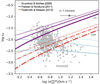 |
Fig. 1. Time-average ϵff measured in 1.5-kpc-wide hexagonal apertures sampling throughout 67 nearby galaxies targeted by PHANGS, as measured by Leroy et al. (2025). Measurements are plotted against the average cloud-scale velocity dispersion |

3.1. A summary of turbulence regulation: Variations in the cloud-scale efficiency per free-fall time ϵff
The two classes of models (described below) shown in Figure 1 share a number of common elements and assumptions, but differences in the way the collapse process is envisioned lead to substantially different predictions in the two cases. Before describing those differences in Sects. 3.1.1 and 3.1.2, we first summarize the basic characteristics of turbulence-regulated star formation models.
In theories of turbulence-regulated star formation (KM05 PN11; FK12; HC11; BM19), the inefficiency of the star formation process taking place within cold dense molecular gas arises from two factors: a high density threshold for collapse ρcrit – set by the competition between the thermal, turbulent, and gravitational energy within the cloud – and the distribution of gas densities imprinted by turbulence above and below this threshold. For a given density PDF, the SFR is derived by integrating the PDF above the critical density for collapse, yielding the so-called core formation efficiency, and then scaling this by a core-to-star efficiency ϵcore, the efficiency with which individual cores form stars. Observations and simulations (Enoch et al. 2008; Sadavoy et al. 2010; Alves et al. 2007; André et al. 2010; Matzner & McKee 2000; FK12) suggest relatively high canonical values ϵcore ∼ 0.3 − 0.5. Thus, the much lower 1–2% efficiencies typical of local and extragalactic clouds are largely a consequence of the inefficiency of the core formation process.
For convenience in comparing different observational estimates of the SFR that are sensitive to different timescales, it is common to consider the star formation efficiency per free-fall time ϵff (sometimes written SFEff) defined as
 (3)
(3)
where the free-fall time tff is that given in Eq. (2), ρ0 is the mean density, s = ln(ρ/ρ0), scrit = ln(ρcrit/ρ0), and the PDF is normalized such that  . Here, tff(ρ0) is the free-fall time at the mean density ρ0, and tcoll(ρ) is the timescale for gas at density ρ to collapse to form cores. This is often written, following KM05, as tcoll = ϕttff, where ϕt is a scaling factor of order unity.
In contemporary turbulence-regulated star formation models, there is some variety in the definition of the critical density scrit (KM05; PN11; HC11) although these tend to be similar in magnitude and behavior (e.g., Burkhart 2018; KM05). Here, we adopt the critical density derived by KM05, identified as the density at which the sonic length (e.g., Federrath et al. 2021) and the Jeans length are comparable, i.e.,
 (4)
(4)
where p ∼ 0.5 is the exponent in the turbulent size-linewidth relation, ϕx is a factor of order unity, and αvir and M are the cloud-scale virial parameter and Mach number, respectively. Throughout this work, we adopt the value ϕx = 1.12, calibrated by KM05 using numerical simulations.
Most model varieties hinge on a common LN density distribution of the form
 (5)
(5)
expected from supersonic isothermal turbulence, where s0 = −1/2σs2 and the PDF width is set by the turbulent properties of the gas according to
 (6)
(6)
where M is the turbulent Mach number, b is the turbulent forcing parameter (ranging from b = 1/3 for solenoidal turbulence to b = 1 for irrotational turbulence), and β = pth/pmag, the ratio of the thermal and magnetic pressures (Federrath et al. 2008; Molina et al. 2012; Federrath & Klessen 2013). In what follows, we adopt b = 0.87 and β = 1 for compatibility with KM05.
Models for the density PDF that include a PL component – to describe the influence of self-gravity and collapse on turbulent motions and the build-up of high-density material – are also becoming more common (see, e.g., Girichidis et al. 2014; Burkhart 2018; BM19; Khullar et al. 2021), as we also consider in this paper.
The most significant differences in predictions for ϵff from model to model originate with the manner in which collapse occurs (FK12) and, in particular, whether the density structure is assumed to be in a steady state. In the following sections, we summarize the two main scenarios and how this translates into the rate of gravitational collapse and star formation.
3.1.1. “Single free fall” KM05 and PN11 predictions: Core formation in a single free-fall time
In the model of KM05, collapse at all densities above ρcrit is assumed to occur at the cloud free-fall rate, i.e., tcoll(ρ) = tff(ρ0). With the density PDF effectively static in this case, as it develops only once in a cloud free-fall time, the gas at density ρ that collapses to form cores also does so only once in a free-fall time. Thus, the so-called MFF factor, tff(ρ0)/tcoll, drops from the integrals and
 (7)
(7)
which becomes
![Mathematical equation: $$ \begin{aligned} \epsilon _{\rm ff,SFF, LN}=\frac{\epsilon _{\rm core}}{2\phi _t}\left[1+\mathrm{erf}\left(\frac{\sigma _s^2-2s_{\rm crit}}{\sqrt{8\sigma _s^2}}\right)\right] \end{aligned} $$](/articles/aa/full_html/2025/08/aa53564-24/aa53564-24-eq37.gif) (8)
(8)
in the case of an LN density PDF, where ϕt is a factor of order unity (KM05). Throughout the remainder of this work, we adopt the value ϕt = 1.9, calibrated by KM05. Given our choice of ϵcore = 0.5, comparison with the predictions examined by FK12, who adopt ϵcore/ϕt = 1, would need to be scaled down by roughly a factor of 4 (∼0.6 dex).
Combined with the high critical density (i.e., as given by Eq. (4)), predictions from this class of single-free-fall (SFF) turbulence-regulated theories successfully yield low, 1–2% efficiencies, even in combination with a relatively high ϵcore ∼ 0.5.
However, as illustrated in Figure 1, these predictions are characterized by a weak dependence on virial parameter and Mach number (with Eq. (8) KM05 predict  ) that is unable to fully capture the wide range in ϵff exhibited by the observed (and simulated) cloud populations in galaxies ranging from normal star-forming disks to starbursts and high-redshift galaxies (where ϵff can reach values as high as 0.1; Usero et al. 2015; Salim et al. 2015; Utomo et al. 2018; and see Figure 1).
This is slightly modified in the scenario envisioned by PN11, who assume that collapse occurs at the free-fall rate at the critical density. In this case, the MFF factor, tff(ρ0)/tcoll = tff(ρ0)/tff(ρcrit), is once again independent of density, but ϵff in Eq. (8) includes an additional multiplicative factor, exp(scrit/2). This greatly enhances the dynamic range in ϵff, but, as illustrated in Figure 1, the predicted increase with increasing Mach number is opposite to the sense implied by extragalactic observations.
3.1.2. “Multi-free-fall” HC11, FK12 predictions: Core formation over multiple free-fall times
As argued by FK12, another avenue to boost the dynamic range of predicted efficiencies is to envision the distribution of gas densities as steady state, continuously replenished over a time trenew, as predicted for turbulent gas by HC11. As a result, collapse at the rate 1/tcoll(ρ)≈1/tff(ρ) can occur multiple times during the period trenew ≈ tff(ρ0).
In this case, the “multi-free-fall” factor, tff(ρ0)/tcoll(ρ)∝tff(ρ0)/tff(ρ), is kept inside the integral in Eq. (3) and
![Mathematical equation: $$ \begin{aligned} \epsilon _{\rm ff,MFF, LN}=\epsilon _{\rm core}\exp \left(\frac{3}{8} \sigma _s^2 \right)\frac{1}{2}\left[1+\mathrm{erf}\left(\frac{\sigma _s^2-s_{\rm crit}}{\sqrt{2\sigma _s^2}}\right)\right], \end{aligned} $$](/articles/aa/full_html/2025/08/aa53564-24/aa53564-24-eq39.gif) (9)
(9)
assuming an LN distribution of densities (FK12).
The factor exp(3σs2/8) in Eq. (9) introduces a strong increase in the predicted ϵff with increasing Mach number. The resulting large dynamic range allows MFF models to reach the highest star formation efficiencies observed (∼0.1; Federrath & Klessen 2012; Salim et al. 2015; Utomo et al. 2018; Dessauges-Zavadsky et al. 2023), better than the KM05 model, which needs to invoke unphysically low Mach numbers (given the weak dependence on virial parameter and Mach number). This yields a qualitative match to the SFRs of different populations, from cores to clouds and starbursts (Salim et al. 2015), systems that are overall more turbulent tend to have relatively high ϵff, as predicted in Eq. (9).
Similar to the PN11 predictions, however, the Mach number dependence at fixed b and cs is opposite to the behavior exhibited by the cloud populations of normal star-forming galaxies (Leroy et al. 2017a; Utomo et al. 2018; see Figure 1). Variations in b and cs (which are taken to be fixed in the right panel of Figure 1 for illustration) might be an avenue for altering the slope of the predicted trend between ϵff and σ. However, with reasonable ranges in these values appropriate for the cold, dense gas in PHANGS targets, the predictions are not modified substantially enough to match the PHANGS measurements.
Matching MFF predictions to observations, moreover, requires a significant ad hoc reduction in the normalization of the model, by one or two orders of magnitude (Salim et al. 2015; Utomo et al. 2018). Indeed, at fixed M, Eq. (9) predicts values for ϵff that are a factor of 10–100 higher than predicted by the single free-fall collapse scenario (Eq. (8)). The factors ϕt and ϕx entering scrit could represent reasonable paths for modifying the normalization, i.e., to apply to galactic scale turbulence that behaves differently than the forced or decaying turbulence in idealized GMC simulations. For now, we choose to adopt the values for these factors from the literature and explore other paths to reduce the normalization of the MFF predictions in Sect. 4. These operate by taking into account how the galactic context of star-forming clouds impacts the output of turbulence-regulated star formation. They thus offer an analytical description to complement what is found in numerical simulations, namely that factors such as feedback, large-scale turbulence, self-gravity, and magnetic fields can reduce the output of MFF predictions to ∼1% (i.e., Federrath 2015; Kretschmer & Teyssier 2020) or impact how closely the efficiencies produced in the simulation match the adopted sub-grid efficiency (Segovia Otero et al. 2025).
4. Modification of MFF models
Recent observational and theoretical insights suggest several avenues for adjusting the predictions of SFF and MFF models to obtain an improved match to observations.
4.1. An overview of the role of gas self-gravity
Already, one of the leading proposals for modifying the predictions of turbulence-regulated star formation models is to add a PL to the assumed density PDF (including Girichidis et al. 2014; Burkhart 2018; Meidt et al. 2020; Burkhart & Mocz 2019; Jaupart & Chabrier 2020). This is a natural expectation for gas that is self-gravitating (Klessen 2000; Kritsuk et al. 2011; Ballesteros-Paredes et al. 2011; Collins et al. 2012; Federrath & Klessen 2013; Burkhart 2018; Jaupart & Chabrier 2020; Donkov et al. 2021, 2022). It also matches the density distributions in local resolved clouds (Kainulainen et al. 2014; Schneider et al. 2015, 2022; Dib et al. 2020; Spilker et al. 2021), which exhibit PL structure (Lombardi et al. 2015; Abreu-Vicente et al. 2015; Alves et al. 2017) down to densities near the cloud edge where the HI-to-H2 transition typically takes place (Σ ∼ 10 − 50 M⊙ pc−2). Although the low-density behavior of observed PDFs is debated (e.g., Schneider et al. 2015; Alves et al. 2017; Körtgen et al. 2019), due in part to the inherent difficulty in distinguishing between low-density cloud material and foreground or background contamination, the observations are compatible with the expectation that the distribution of gas densities is characterized by an LN component transitioning to a PL component at the onset of self-gravitation somewhere near the edges of typical clouds.
As further described in what follows, the PDFs designed in this work to apply under the conditions observed in extragalactic gas (relatively high Mach number and surface density) also contain a prominent PL that begins near the cloud edge and contains a large fraction of cloud material. This prompts other changes from existing descriptions of the star formation process in which the onset of self-gravitation is either accounted for implicitly, by setting the time to rejuvenate the LN density PDF shaped by turbulence (HC11; FK12), or is assumed to occur at higher density in a smaller fraction of the cloud and coincide with core formation (where self-gravity just exceeds thermal and turbulent pressure; BM19). The next three sections discuss additional motivations for these changes and how we incorporate them into turbulence-regulated star formation models.
4.2. Lognormal PDFs with a power-law tail
In hybrid PL+LN density PDFs, the PDF transitions to a PL at the critical density st for self-gravitation, i.e.,
 (10)
(10)
where the normalization N is chosen so that the PDF integrates to unity and C is the amplitude of the PL component, determined by requiring that the density PDF must be continuous (see Burkhart 2018). The slope of the PL tail α is sometimes interpreted in terms of the spherically symmetric radial density profile ρ ∝ r−k, where k = 3/α (Kritsuk et al. 2011; Girichidis et al. 2014).
The PDF proposed by Burkhart (2018, hereafter the smooth-PDF) is formulated in such a way that st is also related to the index of the PL component. Specifically, under the assumption that the density PDF must be smooth (differentiable), Burkhart (2018) find that
 (11)
(11)
where α is the PL index and σs2 is given by Equation (6).
4.2.1. Advantages of hybrid LN+PL PDFs
In the context of turbulence-regulated star formation, adding a PL tail to the density PDF has a number of practical advantages. As shown by Burkhart (2018), PLs are able to increase the dynamic range of predictions at fixed Mach number. They also reduce the output of the models by far enough that BM19 propose that this can remove the need to artificially lower the normalization of MFF predictions (i.e., through ϵcore) in order to match observations (Salim et al. 2015; Utomo et al. 2018).
Moreover, with the functionality of Eq. (11) built in, variations in the PL part of the PDF introduce strong changes in the efficiency per free-fall time, especially when the transition to self-gravitation is used as the critical threshold for collapse and core formation, as argued by BM19. In such a scenario, as st is lowered, the PL slope becomes shallower, and the self-gravitating fraction in the cloud increases, resulting in an increase in ϵff with decreasing α (increasing k).
4.2.2. Efficiencies predicted with smooth LN+PL PDFs
Figure 2 shows the ϵff predicted in single and MFF scenarios with a hybrid smooth-PDF where st = scrit (BM19) and the PL slope is fixed to fall within the range 1.5 < α < 2.5, in line with theoretical predictions (Penston 1969; Shu 1977; Kritsuk et al. 2011; Girichidis et al. 2014; Khullar et al. 2021; Donkov et al. 2021, 2022) and the structure in resolved clouds (e.g., Kainulainen et al. 2014; Spilker et al. 2021; Schneider et al. 2022). The predictions here (as in Fig. 1) assume a thermal sound speed of 0.3 km s−1, ϵcore = 0.5, and a turbulent forcing parameter b = 0.87. In the Burkhart (2018) formulation, ϕt = 1, and we adopt that here when using any LN+PL PDF.
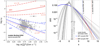 |
Fig. 2. (Left) Predictions for ϵff from turbulence-regulated SF models with a hybrid LN plus PL smooth-PDF proposed by Burkhart (2018) in the SFF (blue) or multi-free-fall (red) scenarios. In these hybrid PDFs, the transition from LN to PL behavior is set to the critical density, st = scrit, as argued by Burkhart & Mocz (2019). A range of PL slopes 1.6 < α < 2.1 set to the range observed by Kainulainen et al. (2014) and Schneider et al. (2022) are indicated by the width of each band. In this example, ϵcore = 0.5, αvir = 5, b = 0.87, and the sound speed cs = 0.3 km s−1. Following Burkhart (2018), we set ϕt = 1. Light gray points show the PHANGS measurements from Leroy et al. (2025), and the dark gray bar and point depict the Dessauges-Zavadsky et al. (2023)z ∼ 1 clumps, repeated from Figure 1. (Right) Illustration of the typical hybrid density PDFs associated with the ϵff predictions in the SFF (blue) and multi-free-fall (red) scenarios at the average cloud-scale velocity dispersion ⟨σc⟩ = 5 km s−1, corresponding to ℳ = 16.7. The blue PDF adopts a PL with slope α = 1.8, which is associated with st = 6.9 (see Eq. (11); marked by the vertical dotted blue line) given the average σc, and yields SFF ϵff predictions such as those shown in blue in the left panel. The red PDF adopts a PL with slope α = 2.7 from the range required to match MFF predictions to the observed ϵff. In this case, the PL starts at st = 11.4 (marked by the vertical dotted red line). Also shown are PDFs with properties matching those measured in local clouds by Schneider et al. (2022). Out of two LNs and two PL components identified by Schneider et al. (2022), only the primary LN and PL components are indicated. These have st = 1 − 2, marked by the narrow vertical gray band, resulting in a kinked appearance. The lighter, wider vertical gray band shows the range in st predicted using Eq. (13) given the observed properties of the plotted regions. |
There are clear differences in the predictions from the two classes of models, with the SFF scenario standing out as providing the closer match to observations. As emphasized by Burkhart (2018), LN+PL predictions can easily reach ϵff = 1 − 2% even when ϵcore ≈ 0.5 − 1. However, here in Figure 2, this has arguably less to do with the addition of the PL (in contrast to the speculation of those authors) than with the SFF nature of the prediction. Similar to SFF predictions generally, the values plotted in Fig. 2 may pass through the PHANGS measurements but fall short of some of the highest observed values ϵff ∼ 10% (Salim et al. 2015; Dessauges-Zavadsky et al. 2023).
The situation is slightly improved in the MFF scenario, with ϵff easily reaching ≳0.1, but the lowest values for ϵff are still out of reach for models with α in the observed range 1.5 < α < 2.5. Adding a PL tail to the PDF still does not solve the issue for PLs with such slopes. To match the measured ϵff in this scenario with relatively high Mach numbers (8 ≳ ℳ ≳ 100) would require significantly steeper PL components with 2.4 < α < 3 (fit in Sect. 6) that are incompatible with the observed clouds or with theory.
4.2.3. Implications of smooth LN+PL PDFs on the dense gas content of clouds
A less readily apparent but nonetheless critical issue with either (MFF or SFF) variety adopting a smooth hybrid PDF is what the transition density between the LN and PL components implies about where gas becomes self-gravitating and how much material is contained at the highest densities.
For gas with Mach numbers as high as observed in extragalactic targets (8 ≲ ℳ ≲ 100 in Figure 1), the st associated with 1.5 < α < 2.5 falls in the range 5–11. These high st are compellingly close to the critical density for collapse in Eq. (4), as highlighted (and leveraged) by BM193. However, such high values unavoidably leave an extended, broad LN component throughout the cloud. This places substantially more mass in intermediate and high density material than when the PL begins (e.g., nearer to the cloud edge), as observed in local clouds. Although we present a fuller study in Sect. 6.4, here we note that clouds with hybrid smooth-PDFs containing a small α ∼ 1.6 PL tail have typically 5–30% of their mass above a density threshold of 103 cm−3 (the effective critical density for HCN, corresponding roughly to the minimum density of the gas responsible for most of the HCN emission from nearby clouds; Leroy et al. 2017b; Neumann et al. 2023). Extragalactic dense gas fractions, on the other hand, are normally observed in the range 1–15% (Gallagher et al. 2018; Neumann et al. 2023).
4.3. Locating the onset of self-gravitation
A number of arguments favor a transition to self-gravitation that is substantially lower than implied by the smooth LN+PL PDFs in Fig. 2, including the observed properties of clouds both in the MW and extragalactic targets. Extragalactic clouds probed over a large range of galactic environments, for one, often show an excess of kinetic energy on the cloud scale, leading to a super-virial dynamical state, as measured by comparing the kinetic energy in the gas to its self-gravity. For the regions under study in Figure 1, 2 ≲ αvir ≲ 10 (Leroy et al. 2025, and as noted in the caption to Figure 1). With a few assumptions, those virial levels can be used to place constraints on the densities needed for gas-self gravity to overcome the turbulent energy. Consider, for illustration purposes, a spherically symmetric cloud with an internal PL density profile ρ ∝ r−k where k = 3/α (Kritsuk et al. 2011; Girichidis et al. 2014). Let the turbulence in the cloud obey the relation σ2 = σ02(r/r0)l, where σ0 is the gas turbulent velocity dispersion on the outer scale r0 and the PL index l ∼ 1 characteristic of the turbulence (i.e., McKee & Ostriker 2007; Heyer & Dame 2015). With these assumptions, the virial parameter at any radius r in the cloud is related to the virial parameter αvir, 0 at radius r0, i.e.,
 (12)
(12)
According to this relation, the virial level αvir, 0 > 1 observed for any cloud on outer scale r0 informs the density ρG needed for gas to become self-gravitating. Letting αvir = 2 mark the threshold for self-gravitation, then
 (13)
(13)
Assuming l = 1 and letting k = 1.5 for illustration, we estimate 1.2 ≲ lnρG/ρ0 ≲ 5 for gas with 3 ≲ αvir ≲ 10 measured in PHANGS targets (Leroy et al. 2025). This lowers to 1 ≲ lnρG/ρ0 ≲ 3 in the case that k = 2.
These values are not only substantially lower than required to match hybrid smooth PDFs to the observed gas properties, they are also much closer to the edge of the cloud, more reminiscent of where the PL starts in local clouds (Schneider et al. 2022). This is arguably consistent with the expectation that the self-gravity of the gas must already become non-negligible somewhere near the cloud edge or the gas would not have started to clump and form the cloud or shape its internal structure, even with the assistance of turbulence. In other words, the defining of the cloud implies that self-gravitation must be happening somewhere not too far from its “edge”.
Later in Sect. 5, we invoke a model that relates the turbulent motions observed on the cloud scale – and the super-virial appearance of the gas – to motion in the galactic potential developing under galactic gravitational forces (Meidt et al. 2018, 2020). We then use that model to propose a specific threshold for the onset of self-gravitation ρG. The alternative to using this model for turbulent gas motions would be to use the observed gas motions directly. We attempt to leave our approach generic enough to accommodate such a choice, leaving the source of the turbulent motion unspecified, or to introduce a different model for the turbulence altogether. However, since our model provides a description for the observed systematic variation in cloud velocity dispersions and virial state (Meidt et al. 2018), we find it a useful framework for interpreting structural variations and how they may be expected to vary with galactic environment (as explored later in Sect. 6.4).
4.3.1. A broad PL tail in a kinked LN+PL PDF
As underlined by the comparison in Figure 2, matching the observed ϵff with a hybrid smooth-PDF in an MFF scenario is difficult when the PL is as shallow (α ∼ 1.5 − 2.5) as implied by observed clouds and as expected from theory (Larson 1969; Penston 1969; Shu 1977; Kritsuk et al. 2011; Girichidis et al. 2014; Jaupart & Chabrier 2020; Khullar et al. 2021). A relaxation of the differentiability criterion4 adopted by Burkhart (2018), however, allows for a more flexible and physical LN+PL model that can match observed PDFs and expectations for the onset of self-gravitation while keeping the predicted star formation efficiency low.
When the differentiability criterion is removed, the hybrid PL+LN PDF has the same normalization as derived by Burkhart (2018), but is no longer restricted to a particular st for a given α (or vice versa). This gives the model the leverage to match observed SFRs with realistic values for α in high Mach number gas all while st is lowered (i.e., below the values required in Figure 2). The resulting PDF has a kink where the PDF transitions from LN to PL, as is often observed in clouds (e.g., Figure 2; Kainulainen et al. 2014; Spilker et al. 2021; Schneider et al. 2022). A major advantage to this sort of non-smooth, kinked hybrid PDF is that it can place significantly less mass at intermediate-to-high densities compared to equal-mass LN and smooth-hybrid counterparts (discussed further in Sect. 6.4), yielding a reduced core formation rate in MFF scenarios. Thus, even in gas with relatively high Mach number, PDFs can yield low enough MFF efficiencies to match observed cloud populations when the LN to PL transition is shifted down and the PDF contains an extended, broad PL.
4.3.2. Relation to the critical density
Inherent to our modification of the hybrid LN+PL PDF from smooth to kinked, we propose that the transition to self-gravitation does not necessarily mark a transition to free-fall collapse, or even coincide with critical density for core formation, i.e., st ≠ scrit. This is based on the idea that self-gravity is capable of shaping the PL even if it does not dominate the energy associated with thermal and turbulent pressure or magnetic fields on some scales. In the presence of these factors, theory and simulations suggest that the action of gravity is to collect material and enhance density contrasts, at most engaging in a slowed or delayed collapse (Girichidis et al. 2014; Xu & Lazarian 2020; Jaupart & Chabrier 2020; Khullar et al. 2021). The result is recorded in the formation of the PL portion of the PDF with a slope that approaches, but does not reach, α = 3/2 characteristic of (pressure-free) free-fall collapse.
In this light, we reserve core formation specifically to the gas with self-gravity large enough to dominate turbulent and thermal energy, located by the critical density scrit. An even higher density threshold within the core boundary presumably marks where self-gravity becomes so strong that gas is able to undergo free-fall collapse to form stars. In that gas, we would expect a second PL PDF slope that most closely approaches α = 1.5 (e.g., Girichidis et al. 2014; Jaupart & Chabrier 2020; Khullar et al. 2021). The onset of this second slope is arguably a factor that impacts the value of the core-to-star efficiency adopted in this work. Since we adopt empirical calibrations of ϵcore and restrict ourselves to describing the phase of core formation, the first, “non-free-fall” PL slope is expected to be most relevant.
4.4. Finite replenishment of density structure
By envisioning the gas as self-gravitating and adding a PL to the PDF, we are also prompted to reconsider how gas structure builds and renews. Our preference to place material in a broad PL tail (so that the PL slope is consistent with the structure in resolved clouds; Kainulainen et al. 2014) is conceptually consistent with the idea of pervasive hierarchical gravitational collapse and turbulence that acts to continuously replenish the density structure in clouds over the course of a cloud free-fall time (HC11; FK12; Girichidis et al. 2014; Appel et al. 2022). That idea leads to the expectation that the time to rejuvenate self-gravitating structures is the timescale over which the PDF is renewed. This is the central idea behind the MFF scenario, which we select as our fiducial model in what follows5. This becomes important for clouds that are not virialized on the cloud scale and instead contain an excess of turbulent energy. For these clouds, structure build-up in the cloud at the outset is through turbulence, i.e., the turbulence crossing time tturb = Rc/σ on the cloud scale Rc is shorter than tff, 0. The rejuvenation time only switches to the free-fall time at higher densities within the cloud, where self-gravity dominates (HC11). By construction, precisely at the self-gravitating threshold the crossing time and the free-fall time are equal. Thus, the free-fall time at the self-gravitating threshold is a measure of the time for self-gravity to renew the cloud’s PDF.
With this view in mind, any factors that weaken self-gravity on the cloud scale are factors that shorten the duration of PDF renewal and thus star formation. In this work (later in Sect. 5), we consider self-gravity in relation to the background galaxy potential, which coordinates turbulent motions with an energy that can exceed self-gravity toward the outer cloud scale. The weakness of self-gravity there acts to halt gravitational collapse below a critical density, reducing the supply of collapsing material that can replenish the high-density PDF. This stops the core (and ultimately star) formation process from proceeding continuously as assumed in MFF models.
A number of factors are also capable of preventing collapse or inhibiting mass transfer from the LN to the PL part of the PDF, such as magnetic fields (Girichidis et al. 2014) or feedback-driven outflows (Appel et al. 2022). As a second modification to conventional turbulence-regulated SF models, we therefore propose to loosen the steady-state assumption that is inherent in typical MFF scenarios. In practice, we do this by limiting the duration of PDF renewal to some time trenew below the cloud free-fall time. Changes in the PDF over the duration of PDF renewal are ignored for the present (i.e., the slope of the density PL is assumed to be constant in time). However, in what follows, we write the density PDF as an explicit function of time, so that models for time variation (e.g., capturing an accelerating ϵffHartmann et al. 2012; Murray & Chang 2015; Lee et al. 2015; Caldwell & Chang 2018) could be incorporated in future applications. Later in Sect. 6.5, we briefly consider evolution in α.
For transparency, in our limited-replenishment scenario, we write ϵff for a cloud observed at any time tobs since the start of the star formation process as
![Mathematical equation: $$ \begin{aligned} \epsilon _{\rm ff}=\frac{\epsilon _{\rm core}}{\phi _t}\frac{1}{t_{\rm obs}}\int _0^{t_{\rm obs}}\left[\int _{s_{\rm crit}}^{\infty }\frac{t_{\rm ff}(\rho _0)}{t_{\rm ff}(\rho )} \frac{\rho }{\rho _0} p(s,t)ds\right]dt, \end{aligned} $$](/articles/aa/full_html/2025/08/aa53564-24/aa53564-24-eq44.gif) (14)
(14)
where the PDF has been normalized such that  and the term in square brackets is the cloud free-fall time multiplied by the core formation rate.
In the event of finite PDF renewal with duration trenew, the integrand in the square brackets is nonzero only up until tstop = trenew, allowing core formation to proceed until tstop. In this work, we wish to examine scenarios in which tstop does not necessarily extend beyond tobs. This is different from the typical approach, in which the core formation process effectively spans a single cloud free-fall time tff(ρ0) (assuming that the cloud’s lifetime is the free fall time) and this tff(ρ0) is also assumed to be roughly equal to or exceed tobs, so that tstop = tff(ρ0)≳tobs. For that case, the ϵff is determined entirely by the term in the square brackets (as in the previous section). For convenience, Table 1 collects the definitions of the various timescales used in this work.
Definitions of timescales considered in this work.
With core formation stopped by a cessation of PDF renewal before a full cloud free-fall time has elapsed, Eq. (14) suggests that
 (15)
(15)
where  is the steady-state efficiency per free-fall time that follows from multiplying ϵcore by the term in the square brackets in Eq. (14) calculated over a cloud free-fall time (i.e., with no stop to core formation). Although write Eq. (15) in terms of a generic tstop, in our preferred view tstop is meant to be set by the free-fall time where the gas becomes self-gravitating.
Equation (14) can be written more generally in terms of the time when the core formation process begins tstart and the visibility timescale of the star formation tracer tsf. For star formation traced by YSOs in galactic clouds, for example, this would be the ∼0.5 Myr duration of the protostellar phase. The visibility timescale is typically longer when the time-averaged SFR within an (extragalactic) cloud population is constructed from kpc-scale observations of extragalactic tracers such as Hα, FUV, and 24 μm emission, following the approach developed by Leroy et al. (2017a) and implemented by Sun et al. (2023), Leroy et al. (2025) (yielding the measurements studied here). As we discuss later in Sect. 6.2.3, in this scenario, when the visibility timescale approaches or exceeds the typical cloud lifetime tlife, then for any individual cloud the minimum tsf = tobs ≈ tlife, or roughly a cloud free-fall time (Chevance et al. 2020).
Clearly, the impact of finite tstop is recognizable as long as tobs > tstop. This correction is therefore potentially most relevant for comparing to extragalactic efficiencies measured with long-timescale star formation tracers, i.e., if a steady state cannot be assumed for the duration of a cloud free-fall time.
5. A physical model for the proposed modifications: The role of galactic environment
One of the main motivations for introducing both of the proposed changes to MFF predictions in the previous section is to model the influence of galactic environment on star-forming clouds. In turbulence-regulated star formation models, the key bottleneck to star formation is the gravitational collapse of gas to form cores, set by the competition between gravity and the energy in thermal and turbulent motions. In Meidt et al. (2020), we hypothesized that a secondary bottleneck acts within clouds, taking place on larger scales and at lower densities. This gas is kinematically coupled to the host galaxy potential and appears super-virial (e.g., Meidt et al. 2018). As a result of the weakness of self-gravity (relative to the total gravitational potential of the galaxy at large), gravitational collapse occurs on timescales that are much longer than the cloud free-fall time. This effectively inhibits self-gravitation and impedes collapse for a portion of the cloud. Only when the gas decouples from the galaxy and achieves virial balance is collapse possible.
With this picture in mind, we let the density threshold for gas to decouple from the galactic potential – also referred to as the threshold for self-gravitation ρG – both mark the density where the density PDF transitions from LN to PL in the hybrid density PDF described in Sect. 4.2 and set the timescale for PDF replenishment following the formalism presented in Sect. 4.4. Given the typical conditions observed in extragalactic star-forming disks, the transition to self-gravitation ρG implied in this scenario places a large fraction of cloud material in a PL component, impacting the efficiency predicted in MFF scenarios as discussed in Sect. 4.3.1.
Again, although the focus here is on the bottleneck model, alternatives can be easily tested using the generic framework presented in Sects. 4.2 and 4.4. Indeed, the bottleneck model is in the family of theories in which self-gravitation decreases with increasing virial parameter (Klessen 2000; Padoan et al. 2016; Jaupart & Chabrier 2020)6. Most generically, we propose parameterizing the effect of super-virial motions by using tstop and setting it to the collapse time in the portion of the gas that reaches a virial (self-gravitating) state. This makes it possible to implement alternative models for how other (nongravitational) processes in the gas, such as SNe feedback (PN11) or magnetic fields (Federrath 2015), impact gas dynamical (virial) state and star formation.
Likewise, the model presented below can be easily modified using alternative prescriptions for ρG. For the present work, the focus is on the threshold for dynamical decoupling from the galactic potential, but star formation efficiencies yielded by PDFs tailored to any number of thresholds can be easilytested.
5.1. The critical density for self-gravitation: Where gas motions decouple from the host galaxy
5.1.1. Practical considerations
In the Meidt et al. (2018, 2020) picture, the threshold density for gas motions to decouple from the galactic potential can be identified by examining the balance between gas self-gravity and the external potential. While it may be possible to compute these potentials numerically (e.g., from an observed or simulated distribution), for practical purposes we seek an analytical threshold that can be easily incorporated into the calculations in Section 3.1. The easiest way to obtain the threshold is thus to make some simplifying assumptions. In particular, within any given local patch of gas, we adopt a triaxial geometry and seek the threshold as the density at some triaxial boundary inside of which the gas self-gravity (counting up all the mass within the triaxial region) exceeds the external potential.
For calculating the balance of potential and/or kinetic energies on the cloud scale, how the mass is arranged within the boundary is less important than the total mass inside that boundary. For simplicity, though, we assume that mass distributions within each triaxial region are cloud-like and fall away in a PL fashion from some central reference point (to pin the integrals for the potential energies) such that ρ ∝ r−k. Of course, real clouds are not close to spherically symmetric or even triaxial nor do they contain only a single overdensity. It is therefore worth emphasizing that this assumption is only invoked for assessing the potential energy near the outer part of the cloud and has little connection to the internal density structure assumed when predicting the SFR. It is therefore not inconsistent with a more realistic, complex arrangement of mass toward higher density (i.e., with multiple peaks). Note too that although the cloud objects envisioned in this scenario would themselves not be filamentary, they could be embedded in larger-scale structures with a filamentary quality (e.g., Smith et al. 2020; Neralwar et al. 2022; Meidt et al. 2023).
The assumption that material within the cloud falls away like ρ ∝ r−k has been fairly common in the literature (e.g., Bertoldi & McKee 1992; Heyer & Dame 2015, and others) and does a fairly good job of matching observed cloud-scale gas motions (Heyer et al. 2009; Hughes et al. 2013; Rosolowsky et al. 2021) under the assumption of virial equilibrium. With this density arrangement, we write the 1D velocity dispersion as
 (16)
(16)
in terms of the gas surface density Σ at radius R in the cloud and the geometric factor,
 (17)
(17)
(Bertoldi & McKee 1992). We chose the velocity dispersion to reflect a direct equivalence between kinetic and potential energy, rather than virial balance, thus introducing the factor of 2 in Eq. (16).
In this arrangement, we can also write a simple expression for the motion in the galactic potential at radius R within the cloud (Meidt et al. 2018, 2020),
 (18)
(18)
where
 (19)
(19)
in the cloud frame, in terms of the circular frequency Ω and the radial and vertical epicyclic frequencies κ and ν that measure the strength of galactic gravitational forces in the radial and vertical direction, respectively (see also Appendix A). Here bk is a geometric factor of order unity derived in Appendix B.
With these assumptions, we write the ratio between self-gravity and the background potential as
 (20)
(20)
 (21)
(21)
The value of this ratio specifically at density ρ0 at the cloud edge is referred to as γ0. In the case that the velocity dispersion in the gas reflects the quadrature sum of the velocity dispersions associated with self-gravity and the background potential (i.e., the two potentials are approximately separable; Meidt et al. 2018), then at minimum, neglecting any nongravitational motions,
 (22)
(22)
The minimum value of γ required for collapse approaching the free-fall rate in the absence of pressure indicates where self-gravity can be expected to dominate over the background potential. Meidt et al. (2018) estimate that this coincides with γ(k = 0)≈2.5, solving the equation of motion for the collapse of a spherical shell in a pressure-free uniform density sphere in the presence of the local galactic potential. To distinguish this criterion from the condition where self-gravity overcomes sources of (thermal, turbulent, or magnetic) pressure in the cloud in order to undergo free-fall collapse, we refer to it as γG. We thus designate γG(k = 0)≈2.5 as the uniform-density criterion for the onset of self-gravitation. This corresponds to αvir ∼ 2.8 according to Eq. (22).
The self-gravitation condition can be adjusted for any arbitrary (nonuniform) density distribution using the definition in Eq. (21), which implies that7
 (23)
(23)
For k = 2, for example, we have a more easily passed threshold with  .
.
A further rearrangement of Eq. (21) yields the threshold density,
 (24)
(24)
where self-gravity dominates the galactic potential, in terms of γG(k) for any k. We note that the threshold here is comparable to the (radially varying) midplane density of the background host galaxy ρgal (Meidt et al. 2020), i.e., ρG ≈ 2.52ν2/(πG)≈ρgal.
In practice, the self-gravitation threshold in a region with density ρ0 can be assigned independently of the cloud internal structure. Rewriting κe as  , Eq. (24) can be expressed as
 (25)
(25)
The equivalence of the two terms on the right-hand side follows from the shared dependence of γG(k) and γ0(k) on k.
Even though γG and ρG depend on k, the ratio ρG/ρ0 is independent of internal structure since ρ0 also varies with k. This leads to a favorable disconnect between the adopted threshold density and the structure of higher density star-forming gas and underscores the relative unimportance of the precise details of our envisioned cloud geometry on our predicted star formation efficiencies. Indeed, in the scenarios of greatest relevance here, ϵff is almost insensitive to the adopted threshold density. For typical molecular gas in nearby galaxies, γ0 ≈ 0.5 − 2 on the cloud scale (Meidt et al. 2020, see also Figure 4). According to Eq. (25), this makes lnρG/ρ0 ≈ 0.4 − 3.2, placing ρG toward the outer edge. Taking the typical observed  M⊙ pc−2 (Leroy et al. 2025) and our adopted h = 100 pc, the average cloud volume density
  M⊙ pc−3. Using this as our estimate of ρ0 in Eq. (25) we find ρG ∼ 3 M⊙ pc−3 (or n ∼ 100 cm−3). The implication of this value of ρG is that most of the cloud material sits in a broad PL tail (see also Alves et al. 2017). As long as the PL tail is dominant like this, in practice the precise location of ρG is less consequential for ϵff than the slope of the PL or the critical density.
5.1.2. A characteristically broad power-law tail: Less mass at intermediate-to-high densities than in lognormal PDFs
Alongside a restriction to PDF replenishment (Sect. 5.2), one of the defining characteristics of the secondary galactic bottleneck is the expectation of a broad PL tail in the density PDF. Considering that this is arguably a general scenario, it is worth emphasizing the number of consequences PLs have for the predicted efficiency of star formation. We illustrate these here using a simple PL PDF of the form
 (26)
(26)
where the normalization CPL is chosen so that  (integrating out to the cloud edge at ρ0).
Compared to an equal-mass LN counterpart, PL PDFs (with exceptions) are characterized by less mass at intermediate-to-high densities, essentially shifting the mass in that regime to both lower and higher densities (see, e.g., the inset in the right panel of Fig. 3). This has the practical consequence of reducing the output of turbulence-regulated star formation models. In the multi-free-fall collapse scenario,
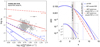 |
Fig. 3. (Left) Predictions for ϵff from turbulence-regulated SF models with the hybrid LN+PL PDF proposed here (Eq. (32)) in the SFF (blue) or multi-free-fall (red) scenarios. In these hybrid PDFs, the transition from LN to PL behavior is set to the density threshold for gas to kinematically decouple from the galaxy (Meidt et al. 2020). A range of PL slopes 1.6 < α < 2.1 set to the range observed by Kainulainen et al. (2014) and Schneider et al. (2022) are indicated by the width of each band. As in Figure 2, here we set ϵcore = 0.5, ϕt = 1, αvir = 5, b = 0.87, and cs = 0.3 km s−1, and use the KM05 critical density in Eq. (4). Here we also adopt a fixed γ = 1. Light gray points show the PHANGS measurements from Leroy et al. (2025), and the dark gray bar and point depict the Dessauges-Zavadsky et al. (2023)z ∼ 1 clumps, repeated from Figure 1. (Right) Illustration of typical hybrid LN+PL density PDFs that can fit the observed ϵff. All cases adopt the average cloud-scale velocity dispersion |

![Mathematical equation: $$ \begin{aligned} \epsilon _{\rm ff,MFF,PL}= \epsilon _{\rm core}\left[\frac{\alpha -1}{\alpha -3/2}\right] \left(\frac{\rho _{\rm crit}}{\rho _0}\right)^{(3/2-\alpha )}, \end{aligned} $$](/articles/aa/full_html/2025/08/aa53564-24/aa53564-24-eq65.gif) (27)
(27)
where the normalization factor in square brackets is equivalent to the geometric factor, (2/3)(3 − k)/(2 − k), derived by Tan et al. (2006) (and used by Meidt et al. 2020) for the spherically symmetric density profile ρ ∝ r−k. Likewise, in the original single free-fall collapse model envisioned by KM05,
 (28)
(28)
For PLs down to α ∼ 1.5, the normalization factor in Eq. (27) is considerably smaller than what follows from integration of an LN PDF. Only at the highest densities or at very low Mach numbers do LNs tend to contain less mass than PLs. As a result, for most PLs in most extragalactic regions, the mass predicted to form stars above the critical density is reduced, ultimately yielding efficiencies back down at the 1% level, even while assuming ϵcore = 1 (see also Burkhart 2018; BM19).
The MFF normalization factor in Eq. (27) is also independent of Mach number, which now functions solely to set the critical density for core formation in this scenario. MFF PL predictions for ϵff thus share the much weaker reverse dependence on Mach number characteristic of the original KM05 models (see Figure 1), rather than the strong increase implied in Eq. (9). These models instead achieve a large dynamic range in ϵff through a strong dependence on PL index α (or k) (Parmentier 2019; Parmentier & Pasquali 2020; Burkhart 2018; Meidt et al. 2020). Resolved local clouds do exhibit a link between ϵff and α (increasing k) similar to that predicted here (Burkhart 2018). In the remainder of this work, in the context of the galactic bottleneck, we interpret variations in extragalactic efficiencies mainly as a result of variations in internal PL structure.
It is worth emphasizing that, such as pure PLs, hybrid non-smooth PDFs with st ∼ 1 − 3 and a PL slope in the observed range α ∼ 1.5 − 2.5 exhibit a deficit of intermediate-density material and a downward-kink appearance characteristically in regions with relatively high Mach numbers (ℳ ∼ 8 − 100) common to cloud-scale observations of extragalactic gas. This presents an interesting contrast to hybrid smooth PDFs in this regime, especially in light of the way gravity is conventionally viewed, i.e., as building a PL on top of an LN, creating structure that resembles a hybrid smooth PDF or a PDF that at most kinks upward (Girichidis et al. 2014; Khullar et al. 2021; Jaupart & Chabrier 2020). At high Mach numbers, such hybrid smooth-PDFs with no kink and st ∼ 1 − 3 would let gravity amplify the density contrasts seeded by turbulence in a way that the PL slope is significantly shallower than α = 1.58 We do not regard such PDFs as necessarily more physical than downward-kink PDFs, particularly because, unlike in simulations, the gas is never in a “non-self-gravitating” initial state with an LN PDF that it proceeds to evolve away from. Self-gravity shapes the gas distribution from the start, immediately shifting any intermediate-density material built up by turbulence to higher densities, shaping the PDF into a PL with α ∼ 1.5 − 2.5. We thus favor the added flexibility of the hybrid non-smooth PDF over the smooth PDF in what follows, although we test both. As discussed later in Sect. 6.4, expanded measurements of dense gas fractions will offer powerful insight into the internal structure of gas, especially at the high Mach numbers typical in clouds outside of the Solar Neighborhood.
5.2. A finite reservoir to undergo collapse and replenish the PDF
An additional characteristic of the secondary galactic bottleneck is its consequence for the renewal of gas density structure over time. Following the arguments in Sect. 4.4, we assume that the density PDF is in a steady state only until the free-fall time at the threshold density for self-gravitation ρG, i.e., tstop = tff, G. For times t > tstop, star formation effectively shuts off, since the remaining gas below ρG is not strongly self-gravitating and unavailable for collapse (until perhaps the cloud environment is modified, introducing a new tstop). These and other timescales used in this work are summarized in Table 1.
Equating tstop with the free-fall time at the threshold ρG given by Eq. (25) chosen for study in this work9, we let
 (29)
(29)
or generically, in terms of the virial parameter αvir,
 (30)
(30)
With these estimates for tstop, predictions for ϵff from all varieties of turbulence-regulated star formation models that take into account the dynamical coupling of gas to the host galaxy potential are thus modified to read
 (31)
(31)
in cases where tstop < tobs ≲ tff(ρ0). Here, ϵff, steady is the value of the efficiency predicted under the assumption that the entire cloud collapses in a cloud free-fall time tff(ρ0) (i.e., the predictions given in the previous sections in the single or MFF scenarios with LN or PL PDFs).
Note that this impact of the secondary bottleneck on the ϵff is only expected to be detectable with long-timescale star formation tracers, tobs > tstop. Galactic clouds likely fall in the second regime above, either because of the short visibility timescales of typical star formation tracers (for which tobs < tstop) or when examined (preferentially) at high densities where the cloud material is already decoupled from motion in the galactic potential (γ0 ≫ γG). Cloud populations probed with longer-visibility extragalactic star formation tracers, on the other hand, tend to fall in the first regime. In such cases, tobs ≈ tff(ρ0) (see Sect. 6.2.3), implying that the SFRs for clouds that contain some amount of material that remains coupled to the galaxy can be measurably lower than prescribed by, for example, Eqs. (9) or (27).
The combination of Eq. (31) with Eq. (27) used for ϵff, steady is equivalent to the prediction presented in Meidt et al. (2020), under the assumption that tobs ∼ tff. In that work, the fraction of the cloud mass available to star formation was expressed in terms of the self-gravitating (or decoupled) gas mass fraction rather than the ratio of timescales introduced here. The predictions in the next section represent an improvement over the Meidt et al. (2020) predictions in several regards. First, whereas previously a fixed core formation efficiency was adopted, here we assign a value that depends on scrit estimated from observed gas properties. Second, in this work we leverage variations in gas density structure to improve the match to observations, rather than adopting a fixed k = 2 as in Meidt et al. (2020).
6. Testing modified turbulence-regulated star formation models with PHANGS
6.1. Summary of the proposed modeling strategy
In this paper, we propose adjustments to turbulence-regulated models of star formation to improve their consistency with observations. Building from the turbulence-regulated threshold for core formation ρcrit as predicted by KM05 and PN11, the main features we propose implementing to match the observed range in ϵff and its variation with cloud-scale gas properties in practice are the following:
-
A broad PL density PDF component to capture the onset of self-gravitation (motivated by observed cloud structure), in practice shifting the overall normalization of the MFF ϵff down and reproducing a weak inverse dependence on Mach number as observed and reproduced by the original SFF KM05 theory.
-
The MFF core formation (or PDF renewal) allowing for greater dynamic range than predicted in SFF scenarios (FK12), spanning from cores to clouds to starbursts.
-
Finite PDF replenishment that limits the duration for star formation to less than a cloud free-fall time, contributing to further reduction in ϵff that can vary locally. The model of renewal we consider in this work is the result of the galactic bottleneck hypothesized by Meidt et al. (2020), which prevents a fraction of cloud material from collapsing to participate in the star formation process.
The second and third of these determine the behavior of the free-fall factor during integration over the density PDF and affect the normalization of the predicted ϵff. The first involves a hybrid PDF identical in form to the model proposed by BM19 (see Eq. (10)), with identical normalization. In what follows, though, we omit the link between the PL index and st required by the differentiability condition adopted by Burkhart (2018). Instead, we test the st value implied by the criterion for self-gravity to dominate the external galactic potential determined by Meidt et al. (2020), i.e., st = sG = ln(ρG/ρ0) with ρG given by Eq. (25). This leaves α as a free parameter.
In general, and as argued in Sect. 4.3.1, in the disks of star-forming galaxies, we expect sG < scrit, with scrit related to the cloud-scale turbulent gas properties (KM05). We thus restrict star formation to gas in the PL tail. The ϵff in this case can be determined by comparing the mass in stars formed, calculated by integrating above ρcrit, to the total gas mass, calculated by integrating the PDF above ρc10. We find
![Mathematical equation: $$ \begin{aligned} \epsilon _{\rm ff}=\epsilon _{\rm core}\frac{\gamma _0}{\gamma _{\rm G}} \frac{C f(\rho _{\rm crit},\alpha )}{\frac{1}{2}\left(1+\text{ erf}\left[\dfrac{(s_t-\sigma _s^2/2)}{\sqrt{2\sigma _s^2}}\right]\right)+C\dfrac{e^{(1-\alpha ) s_t}}{\alpha -1}} , \end{aligned} $$](/articles/aa/full_html/2025/08/aa53564-24/aa53564-24-eq70.gif) (32)
(32)
with
 (33)
(33)
and
 (34)
(34)
This assumes that the LN component of the PDF has width σs given by Eq. (6). For compatibility with the Burkhart (2018) formulation framed around the smooth hybrid LN+PL PDF in Eq. (10), here ϕt is omitted (set to unity).
The factor, γ0/γG, in Eq. (32) reflects the assumption that PDF renewal lasts only until tstop = tff, G < tff, 0, where tff, G is the free-fall time at the density ρG where self-gravity dominates the evolution. Moreover, we set the observed duration of the clouds to their lifetime, which we further assumed to be near the free-fall time at the mean cloud density tff, 0. When the duration of PDF renewal lasts for the full cloud lifetime, tstop = tff, 0, and the factor, γ0/γG, is omitted, as discussed in Sect. 5.2. In the model we choose to test in what follows, ρG is given by the threshold where gas is decoupled from the galactic potential (see Sect. 5). We also use this density to define st, which marks where the density PDF transitions from LN to PL.
As a result of these changes motivated by the introduction of self-gravity, the output efficiency predicted by MFF scenarios is greatly reduced. This is illustrated in Fig. 3, showing predictions from Eq. (32) with ϵcore = 0.5 in both the MFF and SFF scenarios, where (for illustration purposes) a universal threshold ρG is adopted, and the PL slope is fixed to 1.5 < α < 2.5 (as in Figure 2). Compared to either Figure 1 or Figure 2, the MFF predictions provide a closer match to the observed ϵff, all with realistic density PDFs. We call these predictions self-gravitating MFF predictions, or sgMFF predictions, in what follows. In the SFF scenario, on the other hand, exchanging an LN PDF for a broad PL tail leads to too much reduction in ϵff, and the inclusion of the factor, tstop/tobs, describing the galactic bottleneck further increases the discrepancy with the observations. These predictions using a hybrid PDF with a broad PL tail are referred to as sgSFF predictions.
To obtain the best match to the observations, it is clear that the PL slope α must vary systematically throughout the targets, i.e., as a function of σ or related property; no single value of α covers the observed range in ϵff. Although there are models, for example, for the evolution of α over time (e.g., Murray & Chang 2015; Lee et al. 2015; Caldwell & Chang 2018), at this point we prefer not to translate expectations into a dependence on cloud-scale properties and instead opt to fit Eq. (32) to the data to determine the α necessary to match the observations everywhere. By comparing the fitted behavior to independent expectations, we can then qualitatively assess the model (Sect. 6.5).
6.2. Overview of empirical tests
The ϵff model given in Eq. (32) contains a number of factors that all either can be constrained directly with observations of molecular gas on cloud scales or have been shown (observationally or with simulations) to fall within relatively narrow ranges (i.e., b, ϵcore, and α). For the remainder of this section, we describe how we use cloud-scale information constrained by PHANGS (compiled by Sun et al. 2022, 2023 and summarized in Sects. 2.2 and 6.3) to model the time-averaged  measured as in Eq. (1) by Leroy et al. (2025) within kpc-size regions sampling throughout PHANGS targets using a long-visibility (∼10–100 Myr) star formation tracer. For a discussion of the impact of the CO-to-H2 conversion factor on measured cloud properties and the estimated ϵff, as well as the role of the completeness correctionrecommended by Leroy et al. (2025), see Sect. 2.2.
6.2.1. Using the comparison between the model and the observations to constrain α
For comparing to PHANGS observations, we constrain σs, scrit, and st = lnρg/ρ0 empirically (via Eqs. (6), (4), (25), respectively, with the average cloud-scale velocity dispersion and gas volume density measurements as inputs), and leave the PL index as the only remaining variable. With our approach – solving for the value of α that best matches the predictions to the observations – our determinations of α are only as good as the ϵff model, and they inherit the uncertainties associated with factors that are either not well-constrained or incorporated into the model at present. For the extragalactic measurements we consider in this work, the value of tobs, for one, requires additional arguments that may make it subject to greater uncertainty than in the case of shorter-timescale galactic star formation tracers (see Sect. 6.2.3 below). As part of our assessment of the quality of the model in Eq. (32), we thus also examine the α values implied by three alternative ϵff models.
6.2.2. The optimized hybrid LN+PL PDF ϵff models
In addition to testing the ϵff model given by Eq. (32) as both sgMFF and sgSFF, we test the scenario in which the duration of star formation is not restricted to below the cloud free-fall time and assume tstop ≈ tff. We also compare with MFF and SFF predictions using the hybrid smooth-PDF of Burkhart (2018) and Burkhart & Mocz (2019) with st = scrit, adopting identical values for all mutual input parameters. In all four tested models, we adopt b = 0.87 for the turbulent driving parameter, cs = 0.3 km s−1, and ϵcore = 0.5, but comment on the impact of variation in these parameters, where applicable.
The value of α that best matches each of the four models to an observed  is determined using nonlinear least squares regression, specifically the curve_fit routine in the scipy.optimizePython package. The regression is bounded to 1.5 < α < 5 and given an initial input of α = 1.8, the mean value determined for the resolved clouds analyzed by Kainulainen et al. (2014). Note that the width of the LN portion of each fitted model is constrained by the observations, but its normalization and high density extent depend on the fitted α (see Eq. (32)).
With this optimization, estimates of α are determined by fitting to groups/subsets of kpc-scale  measurements. To retain as much leverage on systematic variation in α as possible, we adopt a relatively fine sorting, first by galactocentric radius and then by the mass-weighted average cloud-scale molecular gas surface density
  measured in the associated kpc-sized region, motivated by the large dynamic range in
  present at a given radius (Meidt et al. 2021; Sun et al. 2022; Leroy et al. 2025).
Specifically, after the measurements are sorted into a series of bins of galactocentric radius, each bin is further divided into three groups: below the 30th percentile of the molecular gas surface density distribution at that radius, between the 30th and 70th percentiles, and above the 70th percentile. This division yields groups with roughly equal numbers of (3 or more) measurements per group. In subsequent calculations, all individual measurements in a given group are assigned the same value of α determined for that group. In testing, we find that allowing for systematic variation in α of this kind yields a better match to the observations than when, for example, all measurements at a given radius are used to constrain α. It is worth emphasizing that we have not exhaustively tested alternative sorting schemes (by velocity dispersion, stellar surface density, etc.), and there may be preferable approaches to the one we adopt here. Our main goal is to provide a basic indication of variation in α, wherever present, that can be examined in future work.
6.2.3. Prescriptions for tobs appropriate for long visibility star formation tracers
To compare our full ϵff sgMFF (or sgSFF) model in Eq. (32) to extragalactic measurements, we must assign a representative tobs appropriate for the long visibility timescales of extragalactic kpc-scale star formation tracers (the scenario we describe below does not apply when tsf probes within the lifetimes of the individual clouds). The SFRs constructed on kpc-scales by PHANGS are designed to capture massive star formation over a range of phases and timescales. Each hexagonal kpc region samples multiple instances of the star formation cycle and thus effectively captures star formation over the last tsf ∼ 100 Myr (Leroy et al. 2025). However, in this scenario, when the long visibility timescale tsf exceeds the time to complete any single star formation cycle, or roughly the lifetime of a typical GMC (Chevance et al. 2020), then tobs ≠ tsf. Instead, at maximum tobs = tlife + tno cl, where tlife is the representative cloud lifetime (assumed to vary negligibly locally) and tno cl is the time between cloud formation events11. That is, during the total time, tobs, over which star formation events are “observed”, tno cl denotes the duration of time that gas does not participate in the star formation process. This factor allows us to properly take into account that, whereas our probe of the molecular gas surface density is only telling us about the current generation of clouds, our SFR tracer is also sensitive to the contributions of previous generations of star formation within the same region within the last ∼100 Myr. Note, though, that tno cl is distinct from the time clouds spend in an inert phase (tno sf), which is contained within tlife and is responsible, i.e., for offsetting tstart from the moment of cloud formation or marking the cessation of star formation before a cloud free-fall time has elapsed. We refer to Kruijssen et al. (2019), Chevance et al. (2020, 2022), and Kim et al. (2023) for a description of how different phases of the cloud and star formation cycle can be measured observationally to place constraints on the responsible physical mechanisms.
In practice, we assume for the purposes of the discussion in this paper that the number of clouds within each (high-completeness) 1.5 kpc region is approximately conserved (i.e., that new clouds form at roughly the same rate as old clouds are destroyed), which implies that tno cl is negligible in comparison to tlife. Observational measurements of tlife place it within a factor of 2 of tff (Chevance et al. 2020), suggesting that, with long-visibility tracers, the minimum window of time that each individual cloud is probed can be well approximated by the cloud free-fall time tff(ρ0). This should be good to within a factor of roughly two, but scenarios in which tno cl represents a non-negligible part of the cloud life-cycle may underestimate tobs more strongly.
6.3. Additional empirical constraints from PHANGS
To determine the critical threshold for self-gravitation, ρG, for each “representative cloud” in a given measurement region, we develop an empirical estimate for the parameter γ in Eq. (21) that compares gas self-gravity to the strength of the background galaxy potential on the outer cloud scale Rc.
The self-gravitational potential energy in the numerator of Eq. (21) is written in terms of the gas surface density  on the cloud scale Rc, assuming that the gas is arranged with a triaxial geometry (with cloud vertical extent Zc = qRc, where the axis ratio q ∼ 1) and follows a PL density distribution ρ ∝ r−k.
As derived in Meidt et al. (2018, 2020), on the cloud scale, the background (rotating) potential is written in terms of the effective pressure set up by the gas kinematic response to the associated gravitational forcing. Appendix A describes how we estimate the background potential, using empirical estimates of the underlying stellar density and observed gas rotationalvelocities.
Figure 4 shows the radial distribution of γ measured on the 150-pc cloud scale throughout the target sample, adopting k = 0. Values range from γk = 0 ∼ 0.5 at inner radii to γk = 0 ∼ 2. From the median (mean) γk = 0 = 1.1 (γk = 0 = 1.08), we infer that gas self-gravity and the galactic potential are comparably strong on the cloud scale. This has been suggested earlier using semiempirical galaxy models (Meidt et al. 2018, 2020). As in those models, observed galaxy centers stand out as regions where the galactic potential becomes increasingly important relative to gas self-gravity. These are thus regions where the effective pressure in the gas is dominated by an external component, despite the typically elevated gas surface densities in these zones. As a consequence, the gas density PDF would transition from LN to PL at a higher threshold than in the surrounding disk, signifying that less gas is available to participate in the star formation process over the course of a cloud free-fall time.
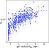 |
Fig. 4. Cloud-scale values of γk = 0 estimated with Eq. (23) shown as a function of galactocentric radius for the subset of hexagonal apertures that sample within galaxies with fitted rotation curves (see Appendix A). Moving inward toward galaxy centers, the influence of the self-gravity of clouds weakens with respect to the galactic potential. |
6.4. Results
Figure 5 summarizes the density structure required to fit PHANGS measurements of  with four different SF models, each pivoting on a hybrid LN+PL density PDF and adopting ϵcore = 0.5. In fitting, the width of the LN portion in all models is set by the local cloud-scale Mach number estimated from the observed gas velocity dispersion, assuming cs = 0.3 km s−1 and b = 0.87. In two out of the three MFF models (our fiducial models, with star formation duration either shortened tstop < tobs or full tstop ≈ tobs, portrayed in black and blue in Figure 5, respectively), the transition density ρt between the LN and PL portions is the same and set to the density where the gas is decoupled from the external potential ρG = ρ0(γG/γ)2.
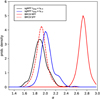 |
Fig. 5. Histograms of the PL slope α in the hybrid (LN plus PL) PDFs that match four different SF models (black, blue, red, and dashed red) to the ϵff measured in PHANGS. The fiducial shortened-duration broad-PL MFF model is shown in black, the full-duration broad-PL MFF model is shown in blue, the Burkhart smooth-PDF MFF model is shown in red, and the Burkhart smooth-PDF SFF model is shown in red with a dashed line. |
In the third MFF model (portrayed by the red line in Fig. 5) as well as in the SFF model (portrayed by the dashed red line in Fig. 5), the transition density ρt is tied to the slope of the PL, as envisioned by Burkhart (2018) (see Eq. (11)), and determined by the α selected during fitting.
6.4.1. Density structure
The α values in the four models are broadly similar, all falling comfortably in the range α = 1.5 − 3. This would correspond to k = 1 − 2 assuming the mass is arranged with a spherically symmetric radial density profile ρ ∝ r−k where k = 3/α (Girichidis et al. 2014). Within this narrow range of α (or k), though, the four models entail appreciably different gas structure. In the MFF smooth-PDF model, which has the highest values for α ∼ 2.5 − 3 (k = 1 − 1.2), the transition from LN to PL is placed at densities ln(ρt/ρ0)∼10 − 15, several orders of magnitude higher than in the fiducial model (ln(ρt/ρ0)∼1 − 3; see Sect. 4) for the regions observed in PHANGS. The PDFs in these smooth-PDF MFF models remain LN for longer (up to higher densities), requiring a dramatic reduction in the highest density content (through a much elevated α) in order to match the observed ϵff.
In the fiducial model, in contrast, the more prominent PL (and reduced high density content) makes it possible to match the ϵff with lower α ∼ 1.6 − 2.5 (higher k ∼ 1.2 − 1.9) that are better consistent with the observed range (k ∼ 1.3 − 2; Kainulainen et al. 2014). This is aided by the limitation to core formation in the shortened duration tstop < tff, 0 model, which allows α to reach the lowest values near α ∼ 1.6 and still match the observed ϵff.
As illustrated in the right panel of Figure 3, the form of the PDF and the role of the PL switches from a high to low Mach number. In the high Mach number regime where the majority of PHANGS observations sit, the PL kinks downward from the LN, bringing MFF models with hybrid PDFs into better agreement with extragalactic observations than pure PLs (see Sect. 5.1.2). In the low Mach number regime, the PL kinks upward, adding high density material relative to the pure LN. The density PDFs for many local clouds (Schneider et al. 2022) tend to show an upward kink, suggesting that in this regime, at a low Mach number, the role of the PL is to enhance the predicted ϵff compared to an equal-mass LN PDF, unlike in extragalactic high Mach number clouds.
6.4.2. Dense gas content
The substantial differences in density structure implied by the four models are explored further in Fig. 6, which shows diagnostics of the density distribution in each model. The bottom row shows the diagnostics for the SFF smooth-PDF model for reference. In the left column, α is plotted against the cloud-scale gas surface density  . The middle column shows the dense gas fractions fd measured from each hybrid PDF above a fixed dense gas density threshold nd = 103 cm−3, near the effective critical density of HCN(1-0) (Leroy et al. 2017b). The right column shows the self-gravitating gas fractions fsg measuring the fraction of gas in the PL portion of the density PDF.
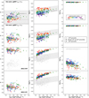 |
Fig. 6. Diagnostics of the hybrid LN plus PL density PDFs that match different MFF (and SFF) SF models to the ϵff values measured in PHANGS. From left to right: Slope of the PL component of the PDF α, the dense gas fraction fd measured above a fixed density threshold (see text), and the self-gravitating fraction fsg measured above the critical density scrit. The top row shows results for PDFs in the fiducial broad PL – the shortened duration model given in Eq. (32) – adopting an MFF scenario. The second row shows results for PDFs in the broad PL – full duration model with tobs = tstop in Eq. (32) also in the MFF scenario. The bottom two rows show MFF (third row) or SFF (fourth row) predictions adopting hybrid smooth-PDFs in the Burkhart formulation, with st = scrit advocated by Burkhart & Mocz (2019). All SF models shown here have assumed ϵcore = 0.5, ϕt = 1, b = 0.87, and cs = 0.3 km s−1, and the critical density given in Eq. (4). As indicated by the color bar in the top right panel, points are color-coded by galactocentric radius (increasing outward, from red to purple). The symbol style denotes relative gas surface density; in all radial bins, regions sitting below the 30th percentile are marked with diamonds, regions between the 30th and 70th are marked with a circle, and regions above the 70th percentile are marked with a cross. The gray points in the bottom row repeat the measurements from the top row. The horizontal gray line (band) in the top left panel shows the mean (full spread) of the PL slopes α observed in local clouds (Kainulainen et al. 2014). The gray band in the middle panels illustrates the relation between the dense gas fraction and the gas surface density fit by Neumann et al. (2023). The width of the band represents the full spread in the fitted data (roughly 3 times the scatter about the fit line). |
Small differences in α amount to notable changes in the amount of the densest material. The top middle panel exhibits good correspondence with the observed values of the dense gas fraction traced by HCN/CO and its empirical relation to gas surface density found by Neumann et al. (2023). That trend resembles the linear relation expected for the fraction of gas above a fixed threshold in clouds with simple PL distributions ρ ∝ r−k with k = 2 (α = 1.5), in particular. The lower α values typical of the fiducial short duration model indeed help match the observed fd level better than the full duration models where α is slightly larger (k is slightly smaller) on average.
In the nominal models (top two rows of Figure 6), the PL represents a large portion of the total mass distribution (roughly a third to a half; see the rightmost column in Figure 6), such that the overall behavior resembles that of pure PLs. In the hybrid smooth-PDF MFF and SFF models (bottom two rows of Figure 6), on the other hand, the PL portion is strongly limited. Self-gravitating fractions are several orders of magnitude lower than in either of the two fiducial models (compare the top two rightmost panels with the bottom two rightmost). As a result, the dense gas fractions for the smooth-PDFs are driven by the LN component. This not only produces a different (weaker) relation to  than in the pure PL case, but tends to produce higher fd values, for the reasons discussed earlier in Sect. 5.1.2, and less scatter as well. So whereas an overall higher α would lower the dense gas fractions on average for pure PL PDFs, in the context of the smooth-PDF models, the overall higher values of α are associated with significantly higher dense gas fractions (i.e., in the third row in Fig. 6).
A higher assumed density threshold could alleviate some of the mismatch between the fd estimated from the MFF and SFF smooth-PDF models and the values observed (and at the same time shift the fiducial models out of agreement with the observed range in α). But the absence of a prominent, shallow PL would still make the MFF and SFF smooth-PDFs defined by Burkhart (2018) less consistent with observed cloud density structure than reproduced with our fiducial models.
In light of these results, we conclude that MFF scenarios provide their best match to observed cloud populations when the density distribution includes a prominent PL component, requiring no artificial reduction in ϵcore. The model for the transition density ρt we examine here is able to satisfy this requirement, but there may be other mechanisms that act similarly. To get a sense for the validity of our proposed model, in the next section we discuss the variations in α that it implies in relation to other expectations for gas density structure.
6.5. Discussion: Systematic variation in α
One of the trends revealed in Figure 6 is the behavior of α at fixed radius (fixed color), which subtly but systematically decreases with decreasing  , moving from regions with locally higher than average surface density (crosses) to regions of locally lower than average surface density (diamonds). All three models show this to some degree, and it is the result of the tight link between efficiency and PL slope predicted by Eq. (32) (and Eq. (27)). Clouds with lower than average surface density but forming stars at the same rate as clouds of higher than average density appear to form stars more efficiently. In our nominal LN+PL model, this higher efficiency is attributed to a higher content of dense gas. The variation in α with
  is largest and clearest in the fiducial short duration model and weakens when the factor, tstop/tobs = γ/γG, is omitted.
In the fiducial model, the decrease in α with decreasing  occurs alongside a clear decrease in α moving toward smaller galactocentric radius (i.e., at fixed surface density percentile). Both the virial level and gas pressure are observed to increase with decreasing galactocentric radius (Sun et al. 2018, 2022). The implication of PL models is therefore that high-pressure, super-virial regions contain gas with broad, shallow density PDFs (see also Burkhart 2018).
Figure 7 shows how α in our fiducial model varies with virial parameter αvir measured in each of the plotted regions, overall exhibiting a stronger link than between α and  . Also shown for reference is the following line:
 (35)
(35)
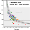 |
Fig. 7. Variation in the PL slope α calculated with the shortened duration model given in Eq. (32) as a function of the cloud-scale virial parameter αvir. Symbol shapes and colors are the same as in Figure 6. The horizontal gray line (band) shows the mean (full spread) of the PL slopes α observed in local clouds (Kainulainen et al. 2014). The reference line given by Eq. (35) with ℛα = 0.23 ± 0.06 is shown in black. Combining the systematic variation of dense gas fraction with virial state implied here together with variations in the critical density (depending on αvir) produces SF efficiencies that match the PHANGS observations in Fig. 1 (see also Fig. C.1 and the discussion in Sect. 6.6). |
chosen to asymptote to α = 1.5 at large αvir. The constant scaling factor, ℛα, here is plotted in Fig. 7 with the value ℛα = 0.23 ± 0.06, chosen from the mean and rms of (α − 1.5)log αvir measured across the plotted data points.
It should be kept in mind that, although the line in Fig. 7 does a surprisingly good job of describing the measurements, it is purely empirical and applies only together with our nominal model. It is a calibration of the relationship between α and αvir needed to match our nominal model for ϵff to the SF in extragalactic clouds observed by PHANGS. Still, it may offer a convenient, testable way to assign the α expected for a given αvir, one based on observations of nearby galaxies that can be examined with observations and simulations.
In Appendix C, we show predictions of the sgMFF model that incorporate the PHANGS-calibrated relation between α and αvir plotted in Figure 7. We emphasize that the trend between α and αvir (or between α and R or  in Figure 6) is a consequence of our choice to let variations in the PL slope drive variations in ϵff. With this in mind, and to offer some validity to the predicted behavior of ϵff examined in Appendix C, below we discuss different physical pictures for how such a trend linking α to αvir might emerge. Here, we first note that the selection biases are expected to have only a small role in shaping the trends recovered in Figs. 6 and 7. We confirm that, in central environments, any clouds with higher α (less dense gas) than typical (αctr ≈ 1.6) would be predicted with Eq. (32) to form stars at rates that are still detectable. Likewise, in the main disk, there appears to be a real absence of clouds with α below the typical αdisk ≈ 2 and their associated higher rates of SF.
6.5.1. Coordination of cloud evolutionary stage
In the first possibility, the density structure reflects the physics of collapse, and the variation in Figs. 6 and 7 is the result of time evolution in the PL slope (i.e., Kritsuk et al. 2011; Federrath & Klessen 2013; Abreu-Vicente et al. 2015; Murray & Chang 2015; Caldwell & Chang 2018). This would be remarkable as it would imply that there are systematic variations in the average evolutionary stage of gas clouds throughout galaxies. Before discussing this possibility further, we note that the current model predictions explicitly neglect the possible time dependence of the PL slope and thus do not strictly account for time evolution. However, as long as we focus on relatively late times in the evolution of the PL, the full evolution can be neglected. Let us consider the scenario in which α asymptotes to αf = 1.5. In this case, the farther the gas is observed from αf, the more a fit to Eq. (32) overestimates the true α, or the degree of overestimation increases at earlier times. To get a sense of the overestimation, we take a pure PL (Eq. (27)) with a time-dependent slope of the form α(t) = a1t−1 + αf and let tstop ≈ tobs ≈ tff(ρ0). Integration of the density PDF in the limit of large scrit yields the expression,
 (36)
(36)
in the MFF scenario. Thus, for α > 3, the true ϵff is more than 4 times lower than the value predicted without time evolution in α. However, for any α currently in the range 1.5 < α < 2.5, the true ϵff is within 1-3 times the time-independent prediction. This translates into less than 10% error in the α determined by fitting to ϵff, from which we conclude that the fitted α should be a close approximation to the true current α for 1.5 < α < 2.5.
With this in mind, the α values in Figs. 6 and 7 determined by fitting the fiducial model to the measured ϵff may indeed probe different stages in the evolution of clouds. To match the systematic variation in α found in this work, the clouds at the innermost radii with low α and high αvir would need to be either more evolved than those at larger galactocentric radii or they would need to evolve systematically faster.
In the former case, the low α in clouds at inner radii would imply that they have had more time to build up their high density interiors than their counterparts in the disk, i.e., because they survive longer. This is typically opposite to the behavior of measured cloud lifetimes, which tend to be shorter where gas densities and velocity dispersions are higher (and thus the free-fall time and crossing time are also systematically shorter).
Short free-fall times could alternatively imply faster evolution, so that central clouds are more often observed with high density tails. This seems the reverse of the correlation implied in Fig. 6 between  (tracking inverse free-fall time), but consistent with a weak link to σ, which is preferentially higher at small R and responsible for the increasing departure from αvir = 1 there.
This may suggest that shorter (turbulent) crossing times are capable of speeding up cloud contraction, helping to rapidly build shallow PL tails. Since cloud properties (including gas velocity dispersion) vary systematically with environment (Sun et al. 2020b; Rosolowsky et al. 2021), this suggests that the galaxy may be playing a role in coordinating the cloud evolutionary state.
6.5.2. Impact of external pressure
In the second possibility, the galaxy’s influence on cloud-scale gas motions has a more direct impact on internal structure through the virial state of the gas. In particular, the increase in αvir (decrease in γ) that occurs with the decrease in α would signify an increasingly large external component to the gas pressure compared to self-gravity (e.g., Heyer et al. 2009; Field et al. 2011; see also Sun et al. 2020b). Numerical simulations suggest that clouds experiencing elevated external pressures contain shallower density profiles (Anathpindika et al. 2018). The decrease in α observed moving inward to dense galaxy centers where the external pressure is systematically elevated (see Fig. 4) is perhaps consistent with this expectation.
A closely related scenario appeals directly to the gravitational forcing exerted by the galaxy to explain super-virial motions, rather than incorporating this influence as an external pressure, although the two are equivalent. In this description, the internal structure of the gas is easily related to the virial level of the gas, as we sketch below.
Consider motion in the rotating frame centered on a cloud orbiting around the galaxy with angular rate Ω. In this frame, the galaxy exerts a radial force κ2r′ a distance r′ from the center of mass (aligned with the galactocentric radius direction) and a vertical force ν2z at vertical distance z. Here (and as given later in Appendix A), κ2 = ∂2Φgal, eff/∂r2 and ν2 = ∂2Φgal, eff/∂z2, where Φeff is the effective potential of the galaxy in the rotating frame.
In the cloud-centered rotating frame, the Euler equation of motion in the radial direction is
 (37)
(37)
where the gas in the cloud has density ρgas, pressure P = ρgasσ2, and
 (38)
(38)
Similarly in the z direction12,
 (40)
(40)
and in the direction y perpendicular to r′,
 (41)
(41)
These expressions can be used to determine the gas density profiles in the r′, y, and z directions that achieve a balance of forces for an assumed velocity dispersion profile. For comparison with the reference isothermal sphere, we consider isothermal gas here below. (The last terms on the right hand sides of Eqs. (42), (40), and (41) can thus be neglected.)
We recall that, in the absence of the external forcing, the equation of motion is written as
 (42)
(42)
in terms of the conventional radial coordinate,
 (43)
(43)
In this case, the equilibrium solution is the cored isothermal density profile,
 (44)
(44)
which behaves as an isothermal profile ∝r−2 outside a constant density core of size,
 (45)
(45)
With the addition of the galactic force terms, the behavior of the equilibrium profile changes. For example, taking the equation of motion in the r′ direction, we see that at r′< a, the constant density of the cored profile also satisfies equilibrium but now with
 (46)
(46)
The same relation follows in the y and z directions.
The prominence of the galactic potential leads to a smaller core at a fixed σ. As a result, more gas is shifted to high densities compared to the nominal equilibrium solution for a (non-singular) self-gravitating cloud.
Outside the core, the equilibrium density profile can be expected to remain well-approximated by r−2 as long as approximately 4πGρsg/κ2 > 1, according to Eqs. (37), (40), and (41). For larger distances, near the cloud edge and beyond, or roughly  , galactic forces dominate equilibrium. As a result, the density in isothermal gasbehaves as
 (47)
(47)
for a given σ, where r02 = σ2/κ2 and z02 = σ2/ν2. Equation (47) is the equilibrium solution to Eqs. (42) and (40) for isothermal gas in the limit of negligible self-gravity. In this scenario, the density of the gas cloud asymptotes to zero, and the mass approaches a finite value, relieving the description here from invoking an external pressure at the edge of a finite mass cloud and the associated Bonnor-Ebert profile.
Compared to equivalent fully self-gravitating clouds, which are able to place more of their mass at large radii in equilibrium, clouds strongly influenced by galactic forces increasing outward from the cloud center (proportional to r) necessarily contain more cloud mass at high density deep in their interiors. The galaxy’s reduction to cloud core in practice makes clouds overall more closely resemble r−2 than when they are more fully self-gravitating, which would in turn make the PL tail of the density PDF overall shallower.
The smaller core contributes to the super-virial appearance of these clouds since the cloud mass and/or radius are changed with respect to their values in equivalent self-gravitating clouds with the same velocity dispersion. Since the cloud mass Mc = 4πa2ρ0Rc (integrating the cored equilibrium profile out to the cloud radius Rc and looking in the limit a/Rc ≪ 1), then at fixed Rc (fixed Mc), a smaller core radius translates to a smaller Mc (larger Rc), both of which raise αvir.
From this perspective, the variation in internal structure and the change in αvir are both consequences of the variation in the galaxy’s influence compared to gas self-gravity across disks. Note that we can envision the pressure needed to balance the weight of the gas in the galactic potential as an external pressure acting on self-gravitating clouds and reach the same conclusion. Extragalactic studies that probe internal structure using proxies such as HCN/CO suggest that the dense gas content systematically increases with decreasing galactocentric radius (e.g., Usero et al. 2015; Gallagher et al. 2018; Querejeta et al. 2019; Jiménez-Donaire et al. 2019; Neumann et al. 2023, 2025), consistent with this picture.
This close link between virial state and internal structure is only expected when the virial state is elevated specifically as a result of motion in the galactic potential, as assumed above. Other scenarios may also lead to an excess of cloud-scale kinetic energy (αvir > 1), such as collisions between gas clouds and/or streams, gas accretion, the interaction or merging of host galaxies, and SF feedback. In those scenarios, the additional forcing experienced by the gas may not elicit the same response as predicted in the presence of galactic forcing, with the consequence that the predicted density profile differs from either Eq. (44) or (47). It should thus be kept in mind that there are scenarios in which an elevated virial state may not necessarily imply that the gas contains a PL with k approaching 2 (α ∼ 1.5) and a relatively high amount of dense material (within which the critical density would also be relatively high (e.g., Eq. (4)), as we find here (Figure 7). When the density PDF is closer to fully LN, it contains even more intermediate-to-high density material than when a PL is also present (see Sects. 4.3.1 and 5.1.2). This suggests that, outside the rotating gas disks of star-forming galaxies, the relation between virial state, internal structure, and dense gas content may be very different than we find here. It is also likely evolving in time, at least partially reflecting the changing influence of the background galaxy.
6.6. Discussion: The impact of changes in α on MFF models and extragalactic star formation
The values of α implied by this work are capable of bringing MFF models into agreement with the observed rates of SF in nearby PHANGS galaxies. It is worth considering what those variations imply about the way galaxies form stars within the context of those models. We recall that we introduce several modifications to MFF models that together reproduce the observed rate of star formation. The first of these is a broad PL that accounts for self-gravity, compensates for changes in virial state, and in practice helps reduce the output of the MFF models overall. The second is the restriction to PDF renewal. Those changes end up making MFF predictions behave, in many ways, closer to the original KM05 models. Consider, for one, the restriction to PDF renewal, which limits the MFF core formation process in time, making it behave similarly to the KM05 model where cores form only once in a cloud free-fall time, rather than continuously. This is in addition to the flexibility added by inclusion of the PL, which allows for changes in dense gas content that can, for instance, compensate for the penalty paid by gas in a super-virial and weakly self-gravitating state. The result is that MFF SFRs are kept from varying as widely as they would if the gas contained a uniform amount of the densest material, mimicking the variation of KM05 predictions and arguably improving the match to observations (see also Appendix C).
While this might tend to suggest that the SF process is better described by the KM05 model than MFF models, context is important. Whereas SF efficiencies may exhibit relatively weak variations in star-forming galaxies (Leroy et al. 2025), where we suspect galactic regulation is active, in other systems, the full flexibility of MFF models and the large dynamic ranges they can achieve may make them preferred (e.g., Salim et al. 2015; Kretschmer & Teyssier 2020; Andalman et al. 2025; see Sect. 3.1). This includes in galaxies at earlier cosmic times (z > 2), before a substantial stellar body has built up to take on its regulatory role, or in gas-rich starburst environments at low or high redshift (e.g., Dessauges-Zavadsky et al. 2023).
In this light, it is even more interesting that the changes in α found in this work imply that, in galaxies on the main sequence, the galaxy leaves little traceable imprint on ϵff; at the same time as the galaxy alters the gas dynamical state, weakening the degree of self-gravitation, it coordinates the dense gas content to yield an overall roughly fixed SF efficiency. Since the normal galactic disk environment is where the bulk of SF since z > 2 has occurred (van der Wel et al. 2014), this implies that the SF process can generally be successfully modeled as taking place in decoupled, turbulent clouds at the basis of the KM05 model. Again, incorporating the galaxy’s influence in the context of an sgMFF model (as in this work), however, may be preferable when attempting to model the ϵff at much earlier cosmic times, or while simultaneously accounting for systematic variations in virial state and dense gas fraction that appear quite common in extragalactic observations.
Altogether, the modifications proposed in this work (Sect. 4) offer a natural way to renormalize the MFF models, by taking into account the self-gravity of the gas and the influence of factors in the environments of star-forming clouds that impact the PDF renewal at the heart of the MFF picture. This includes feedback, magnetic fields, and galactic orbital motions (the latter being the specific focus of this work). The resulting expression for ϵff (Eq. (32)) is thus able to capture what is also found in numerical simulations (e.g., Padoan et al. 2012; Federrath 2015; Appel et al. 2022; Kretschmer & Teyssier 2020), namely that SF proceeds much more slowly than predicted by MFF models when the simulations capture ISM turbulence emerging over a range of scales and track it below the resolution (Semenov et al. 2018, 2024).
Numerical simulations also predict that the recovery of the adopted input efficiency may be sensitive to how efficiencies are (observationally) reconstructed (Grudić et al. 2019; Grisdale et al. 2019; Segovia Otero et al. 2025). The time lag between when SF occurs and when it is observed (given the timescale of the chosen tracer), as well as variations in cloud evolutionary state over kpc-scales, can impact how closely the efficiencies produced in the simulation match the adopted sub-grid efficiency (Segovia Otero et al. 2025). In this light, the analytical model presented here may serve as a useful reference for distinguishing those effects from the impact that realistic galactic-scale turbulence has on the efficiency of SF. In general, cosmological zoom-in simulations (such as VINTERGATAN; Agertz et al. 2021; Renaud et al. 2021; Segovia et al. 2022), as well as idealized simulations of isolated galaxies (see, e.g., Gensior et al. 2020, 2023; Gensior & Kruijssen 2021; Ejdetjärn et al. 2022; Renaud et al. 2024) will continue to shed light on the environmental influences on the turbulent ISM, cloud-scale SF, and their evolution over cosmic time.
7. Summary and conclusions
Recent measurements of the cloud population-averaged (time-averaged) SF efficiency per free-fall time ϵff throughout 67 nearby galaxies with PHANGS (Leroy et al. 2025, see also Fig. 1) show variations with cloud properties that are in tension with most models of turbulence-regulated SF. The implication is that the dependencies of ϵff on turbulence Mach number and gas virial state are different from (and sometimes even the reverse of) theoretical predictions (summarized in Sect. 3.1). In this study, we explored ways to improve the fit of the models to SF. Our modifications (Sect. 4) were built on a growing literature that relates variations in ϵff to the influence of a high-density PL tail that is missing from most models but naturally develops as a consequence of gas self-gravity (Klessen 2000; Kritsuk et al. 2011; Murray & Chang 2015; Burkhart 2018; Jaupart & Chabrier 2020). In these pictures, the ϵff is more sensitive to the slope of the PL tail than to the turbulent Mach number.
All of our modifications, which pivot on the inclusion of self-gravity, also capture the factors, especially those related to the galactic environment, that impact where gravity becomes the dominant factor influencing the evolution and renewal of gas density structure and its associated timescales. We refer to the modified model as the self-gravitating MFF model or sgMFF.
Similar to Burkhart (2018), in this model, we adopted a hybrid density PDF. However, by lifting the requirement that it must be smooth (differentiable), we accommodated a PL tail that is at once broad (extended) and as shallow as indicated by observations of local clouds (Kainulainen et al. 2014; Schneider et al. 2022). For this more realistic broad PL tail, the mass at high density is greatly reduced compared to either a pure LN PDF or the Burkhart smooth-PDF. As a result, it becomes much easier to match MFF models to the low efficiencies observed in local clouds and extragalactic targets without renormalization even when the SF efficiency of dense cores inside the clouds reaches ϵcore = 0.5.
As a physical factor that leads to a broad PL tail, in this study, we considered the balance between gas self-gravity and the energy in motion in the background host galaxy potential (Sect. 5). As described in Sect. 5.1, we let the gas become self-gravitating at densities above where it kinematically decouples from galactic gravitational forces (Meidt et al. 2020, estimated here in Sect. 5.1.1). For typical clouds in nearby galaxies, this transition takes place near the cloud edge, placing it notably in line with where resolved local clouds are shown to exhibit PL behavior (Lombardi et al. 2010, 2015; Kainulainen et al. 2014; Alves et al. 2017; Schneider et al. 2015, 2022, see Sect. 5.1.2).
Another modification suggested by the view of gas self-gravity in the galactic bottleneck picture is related to the duration of PDF replenishment, which is assumed to be continuous in MFF models and lasting until at least a full free-fall time has elapsed. We propose that this duration be shortened when gas in the outer cloud envelope is mostly coupled to the galaxy and unable to collapse, even if slowly (Sect. 5.2). That is, we let PDF renewal be dictated by self-gravity and let the collapse timescale at the self-gravitating threshold set the duration of renewal (see HC11). Star formation feedback and magnetic forces that can impact the dynamical state of the gas would also be factors that can impact the onset of self-gravitation and the replenishment of the density PDF (Girichidis et al. 2014; Appel et al. 2022). Accounting for these factors, we limited the star formation process in the multi-free-fall scenario to some generic time tstop that could be below the cloud free-fall time.
With these choices and our adopted collapse threshold, the SF efficiency predicted with our “self-gravitating” sgMFF model (Sect. 6) is easily reduced to the low levels observed in the local universe, which are also approximately matched by the LN SFF KM05 model. By design, however, our chosen sgMFF model is also able to match the higher efficiencies characteristic of starbursts and clumps at earlier cosmic times (Dessauges-Zavadsky et al. 2023; and see Salim et al. 2015 and references therein). In doing so, our model takes advantage of the added leverage of the PL slope α, which we find is the greatest factor impacting the precise value predicted for ϵff.
Matching PHANGS observations requires systematic variation in α across galaxies. To obtain some insight into the processes that might be responsible for variations in α, we fit several models to the PHANGS data and solved for α (Sect. 6.4). Both our fiducial sgMFF model (broad PL plus limited MFF replenishment) and the smooth-PDF with SFF collapse proposed by Burkhart (2018) can be fit with PL slopes that are fully consistent with the range observed in local clouds. The PL behavior in the two models is otherwise quite different. We quantified these differences using the fraction of gas above a fixed density threshold (selected to be near the effective critical density for HCN) and the self-gravitating fraction as structural diagnostics. We find that the broad PL PDFs entail considerably lower dense gas fractions than the smooth-PDFs where the LN component is more dominant. This brings the former into closer agreement with extragalactic dense gas fractions probing comparable density contrasts (e.g., Gallagher et al. 2018; Neumann et al. 2023).
In either of the two best-fitting models, the PL slope needed to match PHANGS measurements exhibits an increase with increasing  and a decrease with increasing virial parameter. Together with the sensitivity of cloud properties and virial state to galactic environment highlighted by recent work (Sun et al. 2018, 2020a, 2022; Liu et al. 2021; Rosolowsky et al. 2021; Meidt et al. 2021; Lu et al. 2024), this suggests that the host galaxy helps regulate the internal structure of clouds. There are a few avenues for how this might occur, as discussed in Sect. 6.5. For one, the total, deeper potential supports “super-virial” motions in the gas sometimes discussed in terms of an external pressure (e.g., Meidt et al. 2018; Sun et al. 2018, 2020b, see 6.5.2). According to the numerical study of Anathpindika et al. (2018), this external pressure might then act to lower the PL slope. In support of this scenario, we examined the Euler equation of motion to infer how gas responds in the presence of galactic forces. Since these forces increase with distance from the cloud center, more of the cloud mass is forced to high density in the cloud interior than characteristic of fully self-gravitating clouds. Clouds embedded in a strong background galactic potential appear closer to the isothermal α ≈ 1.5 expectation than their self-gravitating counterparts, which can contain a broader constant density core that steepens the density PDF PL tail.
Another possibility is that the galaxy coordinates the average cloud evolutionary state in any given region, preferentially giving clouds in galaxy centers the opportunity to build PL tails either faster or for longer periods than in the main disk environment (Sect. 6.5.1). Since cloud lifetimes tend to be shorter (rather than longer) in centers, we suggest that the enhanced nonthermal motions characteristic of galaxy centers, which translate into shorter turbulent crossing times, could signify that cloud evolution is sped up, supporting the rapid development of a PL tail. In this way, the time evolution predicted for the PL slope (e.g., Kritsuk et al. 2011; Federrath & Klessen 2013; Girichidis et al. 2014; Abreu-Vicente et al. 2015; Murray & Chang 2015; Caldwell & Chang 2018) within clouds would have recoverable influence on extragalactic SF efficiencies.
In either case, our results suggest that galaxy regulation may be key to modeling extragalactic SF, even if the signs of this regulation may not always be apparent. The two functions we attribute to the galaxy – setting the amount of dense material in gas, which it simultaneously shifts to a super-virial, weakly self-gravitating state (restricting PDF renewal) – have competing influences on ϵff (Sect. 6.6). The result, within the context of our nominal sgMFF models, is that the galaxy’s influence on the SF efficiency is imperceptible in practice. As an additional consequence, clouds, in producing stars, behave nearly as envisioned in the KM05 model, i.e., as roughly virialized objects in which turbulence regulates SF output in the course of a cloud free-fall time. Thus, despite outward signs that the gas is not fully self-gravitating and rather is coupled to the galaxy (i.e., exhibiting deviations in virial state and internal structure), SF in main sequence galaxies can be readily modeled as approximately virial, as envisioned by KM05, arguably thanks to the galaxy’s influence.
For modeling SF beyond the galaxy’s regulatory influence, on the other hand, the full flexibility of the MFF class of models (with or without including a PL component in the gas density PDF) may offer the preferable choice. This includes starbursts with locally high gas fractions and at earlier cosmic times, before a substantial stellar body has built up. In both cases, with Eq. (32) we predict considerably higher efficiencies than when the galaxy regulates the SF process. The MFF models are also indispensable for predicting SF efficiencies, while simultaneously treating variations in α and virial states with galactic environment, as employed in this work.
To test the role of the galaxy in the regulation of SF speculated on here, it is necessary to independently establish a connection between α and environment, i.e., through the study of extragalactic multiline surveys that probe gas over a range of densities (from centers to disks). Multi-scale numerical simulations of star-forming gas in the context of a fully evolving galaxy potential, with feedback and chemistry included, is also key. The ability to trace the full budget of SF, (e.g., with radio continuum observations), will help refine this view further, as will the recovery of SF at early times and on small scales (e.g., with JWST), allowing for measurements of the efficiency at different stages to be uncovered. Such datasets will continue to shed light on the relationship between the SF efficiency, gas structure, and galactic environment.
Following Sun et al. (2023) and Leroy et al. (2025), these measurements are extracted from maps of Σmol and ΣSFR that have been convolved to share a matched Gaussian kernel with a FWHM equal to the hex diameter and then sampled at the hex center.
Conservatively assuming αvir ∼ 1, 4 < scrit < 8 for 5 ≳ ℳ ≳ 8.
Whereas the distribution function, or cumulative density function, needs to be continuous and differentiable, the density PDF does not.
With their choice of st = scrit, BM19, in contrast, implement what is essentially an SFF scenario to predict SFEs.
Now that we allow self-gravitation to explicitly shape the PDF and add a PL, it also becomes relevant to account for the time it takes for structure to rejuvenate in comparison to the cloud’s lifetime τ ≈ tff(ρ0).
In the Meidt et al. (2018, 2020) picture, turbulent motions in the gas, and thus its virial state, are modeled as the equilibrium gas response in the presence of the external host galaxy potential (together with self-gravity). The larger the galactic component, the more weakly self-gravitating and apparently “super-virial” the gas becomes, reducing its ability to collapse and form stars.
This is in contrast to the scaling ak/5 erroneously suggested earlier by Meidt et al. (2018).
Conversely, at high Mach numbers (ℳ ∼ 8 − 100), hybrid smooth-PDFs with α ∼ 1.5 − 2.5 but no kink would need to have st ∼ 4 − 20, which lies well beyond the typical estimates for scrit for the highest Mach numbers.
Meidt et al. (2020) found that the rate of collapse, tG at ρG, is slightly longer than the free-fall time.
Following convention, the hybrid PDF is normalized so that  . However, unlike in the case of a pure LN PDF that is assumed to be centered at s0 = −σs2/2, the mass
  in the case of the hybrid normalized PDF (either smooth or non-smooth) is not unity.
Note that this procedure is mathematically equivalent to setting tobs = tsf while reducing the estimated SFR by a factor of 1/(tlife + tno cl) to account for the fact that our SFR tracer is sampling multiple generations of star formation.
As discussed in Sect. 5, the galactic force terms in Eqs. (37), (40) and (41) lead to oscillatory motion within the cloud that sets up a velocity dispersion and can be envisioned as an effective pressure, Pgal. For motion in the r′ direction that obeys the equation of motion  (in the absence of gas self-gravity), for example, we set
  and rewrite the equation of motion as
 (39)
(39)
Following Meidt et al. (2018) we can then define the effective velocity dispersion σgal2 = Pgal/ρ for an assumed gas density distribution ρ (see Appendix B). Alternatively, we can determine the gas density profile associated with a given σgal. For a constant (isothermal) velocity dispersion, the equilibrium scenario represented by Eq. (39) yields the density profile given in Eq. (47) treating the force balance (or equilibrium) in the vertical direction analogously to that in the radialdirection.
The agreement is not perfect as a result of the grouping strategy we used during fitting, which assigns the α determined for any given group of regions to each of the regions in that group.
Acknowledgments
This work was carried out as part of the PHANGS collaboration. We would like to thank the referee for a detailed review and insightful comments. SCOG and RSK acknowledge financial support from the European Research Council via the ERC Synergy Grant “ECOGAL” (project ID 855130), from the German Excellence Strategy via the Heidelberg Cluster of Excellence (EXC 2181 – 390900948) “STRUCTURES”, and from the German Ministry for Economic Affairs and Climate Action in project “MAINN” (funding ID 50OO2206). They are also grateful for computing resources provided by the Ministry of Science, Research and the Arts (MWK) of the State of Baden-Württemberg through bwHPC and the German Science Foundation (DFG) through grants INST 35/1134-1 FUGG and 35/1597-1 FUGG, and also for data storage at SDS@hd funded through grants INST 35/1314-1 FUGG and INST 35/1503-1 FUGG. JG gratefully acknowledges funding via STFC grant ST/Y001133/1. JDH gratefully acknowledges financial support from the Royal Society (University Research Fellowship; URF/R1/221620). This paper makes use of the following ALMA data, which have been processed as part of the PHANGS–ALMA CO (2-1) survey: ADS/JAO.ALMA#2012.1.00650.S, ADS/JAO.ALMA#2013.1.00803.S, ADS/JAO.ALMA#2013.1.01161.S, ADS/JAO.ALMA#2015.1.00121.S, ADS/JAO.ALMA#2015.1.00782.S, ADS/JAO.ALMA#2015.1.00925.S, ADS/JAO.ALMA#2015.1.00956.S, ADS/JAO.ALMA#2016.1.00386.S, ADS/JAO.ALMA#2017.1.00392.S, ADS/JAO.ALMA#2017.1.00766.S, ADS/JAO.ALMA#2017.1.00886.L, ADS/JAO.ALMA#2018.1.01321.S, ADS/JAO.ALMA#2018.1.01651.S, ADS/JAO.ALMA#2018.A.00062.S, ADS/JAO.ALMA#2019.1.01235.S, ADS/JAO.ALMA#2019.2.00129.S, ALMA is a partnership of ESO (representing its member states), NSF (USA), and NINS (Japan), together with NRC (Canada), NSC and ASIAA (Taiwan), and KASI (Republic of Korea), in cooperation with the Republic of Chile. The Joint ALMA Observatory is operated by ESO, AUI/NRAO, and NAOJ. The National Radio Astronomy Observatory is a facility of the National Science Foundation operated under cooperative agreement by Associated Universities, Inc.
References
- Abreu-Vicente, J., Kainulainen, J., Stutz, A., Henning, Th., & Beuther, H. 2015, A&A, 581A, 74 [Google Scholar]
- Agertz, O., Renaud, F., Feltzing, S., et al. 2021, MNRAS, 503, 5826 [NASA ADS] [CrossRef] [Google Scholar]
- Alves, J., Lombardi, M., & Lada, C. J. 2007, A&A, 462, 17 [Google Scholar]
- Alves, J., Lombardi, M., & Lada, C. J. 2017, A&A, 606, L2 [NASA ADS] [CrossRef] [EDP Sciences] [Google Scholar]
- Anathpindika, S., Burkert, A., & Kuiper, R. 2018, MNRAS, 474, 1277 [Google Scholar]
- Andalman, Z. L., Teyssier, R., & Dekel, A. 2025, MNRAS, 540, 3350 [Google Scholar]
- André, P., Men’shchikov, A., Bontemps, S., et al. 2010, A&A, 518, 102 [Google Scholar]
- Appel, S. M., Burkhart, B., & Semenov, V. 2022, ApJ, 927, 75 [NASA ADS] [CrossRef] [Google Scholar]
- Ballesteros-Paredes, J., Vázquez-Semadeni, E., Gazol, A., et al. 2011, MNRAS, 416, 1436 [NASA ADS] [CrossRef] [Google Scholar]
- Barnes, A., Glover, S., Kreckel, K., et al. 2021, MNRAS, 508, 5362 [NASA ADS] [CrossRef] [Google Scholar]
- Bertoldi, F., & McKee, C. F. 1992, ApJ, 395, 140 [NASA ADS] [CrossRef] [Google Scholar]
- Burkhart, B. 2018, ApJ, 863, 118 [CrossRef] [Google Scholar]
- Burkhart, B., & Mocz, P. 2019, ApJ, 879, 129 [NASA ADS] [CrossRef] [Google Scholar]
- Caldwell, S., & Chang, P. 2018, MNRAS, 474, 4818 [Google Scholar]
- Chevance, M., Kruijssen, J. M. D., Hygate, A., et al. 2020, MNRAS, 493, 2872 [NASA ADS] [CrossRef] [Google Scholar]
- Chevance, M., Kruijssen, J. M. D., Krumholz, M. R., et al. 2022, MNRAS, 509, 272 [Google Scholar]
- Choi, W., Liu, L., Bureau, M., et al. 2023, MNRAS, 522, 4078 [Google Scholar]
- Choi, W., Bureau, M., Liu, L., et al. 2024, MNRAS, 531, 4045 [Google Scholar]
- Collins, D. C., Kritsuk, A. G., Padoan, P., et al. 2012, ApJ, 750, 13 [NASA ADS] [CrossRef] [Google Scholar]
- Colombo, D., Hughes, A., Schinnerer, E., et al. 2014, ApJ, 784, 3 [NASA ADS] [CrossRef] [Google Scholar]
- Dessauges-Zavadsky, M., Richard, J., & Combes, F. 2023, MNRAS, 519, 6222 [NASA ADS] [CrossRef] [Google Scholar]
- Dib, S., Bontemps, S., Schneider, N., et al. 2020, A&A, 642, 177 [Google Scholar]
- Dobbs, C., & Pringle, J. E. 2013, MNRAS, 432, 653 [NASA ADS] [CrossRef] [Google Scholar]
- Dobbs, C., Burkert, A., & Pringle, J. E. 2011, MNRAS, 413, 2935 [Google Scholar]
- Dobbs, C., Rosolowsky, E., Pettitt, A., et al. 2019, MNRAS, 485, 4997 [Google Scholar]
- Donkov, S., Stefanov, I. Z., Veltchev, T. V., & Klessen, R. S. 2021, MNRAS, 505, 3655 [NASA ADS] [CrossRef] [Google Scholar]
- Donkov, S., Stefanov, I. Z., Veltchev, T. V., & Klessen, R. S. 2022, MNRAS, 516, 5726 [Google Scholar]
- Duarte-Cabral, A., & Dobbs, C. L. 2016, MNRAS, 458, 3667 [NASA ADS] [CrossRef] [Google Scholar]
- Ejdetjärn, T., Agertz, O., Östlin, G., Renaud, F., & Romeo, A. B. 2022, MNRAS, 514, 480 [CrossRef] [Google Scholar]
- Enoch, M. L., Evans, N. J., Sargent, A. I., et al. 2008, ApJ, 684, 1240 [Google Scholar]
- Evans, N. J., Kim, J.-G., & Ostriker, E. 2022, ApJ, 929, L18 [NASA ADS] [CrossRef] [Google Scholar]
- Federrath, C. 2015, MNRAS, 450, 4035 [Google Scholar]
- Federrath, C., & Klessen, R. S. 2012, ApJ, 761, 156 [Google Scholar]
- Federrath, C., & Klessen, R. S. 2013, ApJ, 763, 51 [Google Scholar]
- Federrath, C., Klessen, R. S., & Schmidt, W. 2008, ApJ, 688, 79 [Google Scholar]
- Federrath, C., Klessen, R. S., Iapichino, L., & Beattie, J. R. 2021, Nat. Astron., 5, 365 [NASA ADS] [CrossRef] [Google Scholar]
- Field, G. B., Blackman, E. G., & Keto, E. R. 2011, MNRAS, 416, 710 [NASA ADS] [Google Scholar]
- Gallagher, M. J., Leroy, A. K., Bigiel, F., et al. 2018, ApJ, 868, L38 [CrossRef] [Google Scholar]
- Gensior, J., & Kruijssen, J. M. D. 2021, MNRAS, 500, 2000 [Google Scholar]
- Gensior, J., Kruijssen, J. M. D., & Keller, B. W. 2020, MNRAS, 495, 199 [NASA ADS] [CrossRef] [Google Scholar]
- Gensior, J., Davis, T. A., Bureau, M., et al. 2023, MNRAS, 526, 5590 [Google Scholar]
- Girichidis, P., Konstandin, L., Whitworth, A., & Klessen, R. 2014, ApJ, 781, 91 [CrossRef] [Google Scholar]
- Girichidis, P., Offner, S. S. R., Kritsuk, A. G., et al. 2020, Space Sci. Rev., 216, 68 [NASA ADS] [CrossRef] [Google Scholar]
- Grisdale, K., Agertz, O., Renaud, F., et al. 2019, MNRAS, 486, 5482 [NASA ADS] [CrossRef] [Google Scholar]
- Grudić, M. Y., Hopkins, P. F., Lee, E. J., et al. 2019, MNRAS, 488, 1501 [CrossRef] [Google Scholar]
- Hartmann, L., Ballesteros-Paredes, J., & Heitsch, F. 2012, MNRAS, 420, 1457 [Google Scholar]
- Hennebelle, P., & Chabrier, G. 2011, ApJ, 743, 29 [Google Scholar]
- Henshaw, J. D., Kruijssen, J. M. D., Longmore, S. N., et al. 2020, NatAs, 4, 1064 [Google Scholar]
- Heyer, M., & Dame, T. M. 2015, ARA&A, 53, 583 [Google Scholar]
- Heyer, M., Krawczyk, C., Duval, J., & Jackson, J. M. 2009, ApJ, 699, 1092 [Google Scholar]
- Hughes, A., Meidt, S. E., Colombo, D., et al. 2013, ApJ, 779, 46 [NASA ADS] [CrossRef] [Google Scholar]
- Jaupart, E., & Chabrier, G. 2020, ApJ, 903, 2 [NASA ADS] [CrossRef] [Google Scholar]
- Jiménez-Donaire, M. J., Bigiel, F., Leroy, A. K., et al. 2019, ApJ, 880, 127 [CrossRef] [Google Scholar]
- Kainulainen, J., Federrath, C., & Henning, T. 2014, Science, 344, 183 [NASA ADS] [CrossRef] [Google Scholar]
- Khullar, S., Federrath, C., Krumholz, M. R., & Matzner, C. 2021, MNRAS, 507, 4335 [NASA ADS] [CrossRef] [Google Scholar]
- Kim, J.-G., Kim, W.-T., & Ostriker, E. C. 2018, ApJ, 859, 68 [NASA ADS] [CrossRef] [Google Scholar]
- Kim, J., Chevance, M., Kruijssen, D., et al. 2023, ApJ, 944, L20 [NASA ADS] [CrossRef] [Google Scholar]
- Klessen, R. S. 2000, ApJ, 535, 869 [NASA ADS] [CrossRef] [Google Scholar]
- Klessen, R. S., & Glover, S. C. O. 2016, Star Formation in Galaxy Evolution: Connecting Numerical Models to Reality, Saas-Fee Advanced Course (Springer-Verlag Berlin Heidelberg), 43, 85 [NASA ADS] [CrossRef] [Google Scholar]
- Körtgen, B., Federrath, C., & Banerjee, R. 2019, MNRAS, 482, 5233 [Google Scholar]
- Kretschmer, N., & Teyssier, R. 2020, MNRAS, 492, 1385 [Google Scholar]
- Kritsuk, A. G., Norman, M. L., & Wagner, R. 2011, ApJ, 727, 20 [NASA ADS] [CrossRef] [Google Scholar]
- Kruijssen, J. M. D., & Longmore, S. 2014, MNRAS, 439, 3239 [NASA ADS] [CrossRef] [Google Scholar]
- Kruijssen, J. M. D., Schruba, A., Chevance, M., et al. 2019, Nature, 569, 519 [NASA ADS] [CrossRef] [Google Scholar]
- Krumholz, M. R., & McKee, C. F. 2005, ApJ, 630, 250 [Google Scholar]
- Lang, P., Meidt, S. E., Rosolowsky, E., et al. 2020, ApJ, 897, 122 [CrossRef] [Google Scholar]
- Larson, R. B. 1969, MNRAS, 145, 271 [Google Scholar]
- Lee, E. J., Chang, P., & Murray, N. 2015, ApJ, 800, 49 [NASA ADS] [CrossRef] [Google Scholar]
- Leroy, A. K., Schinnerer, E., Hughes, A., et al. 2017a, ApJ, 846, 71 [Google Scholar]
- Leroy, A. K., Usero, A., Schruba, A., et al. 2017b, ApJ, 835, 217 [NASA ADS] [CrossRef] [Google Scholar]
- Leroy, A. K., Schinnerer, E., Hughes, A., et al. 2021, ApJS, 257, 43 [NASA ADS] [CrossRef] [Google Scholar]
- Leroy, A. K., Sun, J., Meidt, S. E., et al. 2025, ApJ, 985, 14 [Google Scholar]
- Liu, L., Bureau, M., Blitz, L., et al. 2021, MNRAS, 505, 4048 [NASA ADS] [CrossRef] [Google Scholar]
- Lombardi, M., Alves, J., & Lada, C. 2010, A&A, 519, 7 [Google Scholar]
- Lombardi, M., Alves, J., & Lada, C. 2015, A&A, 576, 1 [Google Scholar]
- Lu, A., Haggard, D., Bureau, M., et al. 2024, MNRAS, 531, 3888 [Google Scholar]
- Mac Low, M.-M., & Klessen, R. S. 2004, Rev. Mod. Phys., 76, 125 [Google Scholar]
- Matzner, C. D., & McKee, C. 2000, ApJ, 545, 364 [NASA ADS] [CrossRef] [Google Scholar]
- McKee, C., & Ostriker, E. C. 2007, ARA&A, 45, 565 [NASA ADS] [CrossRef] [Google Scholar]
- Meidt, S. E., Hughes, A., Schinnerer, E., et al. 2013, ApJ, 779, 45 [NASA ADS] [CrossRef] [Google Scholar]
- Meidt, S. E., Hughes, A., Dobbs, C., et al. 2015, ApJ, 806, 72 [NASA ADS] [CrossRef] [Google Scholar]
- Meidt, S. E., Leroy, A., Rosolowsky, E., et al. 2018, ApJ, 854, 100 [NASA ADS] [CrossRef] [Google Scholar]
- Meidt, S. E., Glover, S. C. O., Kruijssen, J. M. D., et al. 2020, ApJ, 892, 73 [CrossRef] [Google Scholar]
- Meidt, S. E., Leroy, A., Querejeta, M., et al. 2021, ApJ, 913, 113 [NASA ADS] [CrossRef] [Google Scholar]
- Meidt, S. E., Rosolowsky, E., Sun, J., et al. 2023, ApJ, 944, L18 [CrossRef] [Google Scholar]
- Molina, F. Z., Glover, S. C. O., Federrath, C., & Klessen, R. S. 2012, MNRAS, 423, 2680 [NASA ADS] [CrossRef] [Google Scholar]
- Murray, N., & Chang, P. 2015, ApJ, 804, 44 [NASA ADS] [CrossRef] [Google Scholar]
- Neralwar, K. R., Colombo, D., Duarte-Cabral, A., et al. 2022, A&A, 664, 84 [Google Scholar]
- Neumann, L., Gallagher, M. J., Bigiel, F., et al. 2023, MNRAS, 521, 3348 [NASA ADS] [CrossRef] [Google Scholar]
- Neumann, L., Jimenez-Donaire, M. J., Leroy, A. K., et al. 2025, A&A, 693, 13 [Google Scholar]
- Ostriker, E. C., McKee, C., & Leroy, A. K. 2010, ApJ, 721, 975 [CrossRef] [Google Scholar]
- Padoan, P., & Nordlund, A. 2011, ApJ, 730, 40 [NASA ADS] [CrossRef] [Google Scholar]
- Padoan, P., Haugbølle, T., & Nordlund, A. 2012, ApJ, 759, L27 [NASA ADS] [CrossRef] [Google Scholar]
- Padoan, P., Federrath, C., Chabrier, G., et al. 2014, in Protostars and Planets VI, eds. H. Beuther, R. S. Klessen, C. P. Dullemond, & T. Henning (Tucson: University of Arizona Press), 77 [Google Scholar]
- Padoan, P., Pan, L., Haugbølle, T., & Nordlund, A. 2016, ApJ, 822, 11 [NASA ADS] [CrossRef] [Google Scholar]
- Parmentier, G. 2019, ApJ, 887, 179 [NASA ADS] [CrossRef] [Google Scholar]
- Parmentier, G., & Pasquali, A. 2020, ApJ, 903, 56 [CrossRef] [Google Scholar]
- Penaloza, C. H., Clark, P. C., Glover, S. C. O., & Klessen, R. S. MNRAS, 475, 1508 [Google Scholar]
- Penston, M. V. 1969, MNRAS, 144, 425 [NASA ADS] [CrossRef] [Google Scholar]
- Pettitt, A., Dobbs, C. L., Baba, J., et al. 2020, MNRAS, 498, 1159 [Google Scholar]
- Querejeta, M., Schinnerer, E., Schruba, A., et al. 2019, A&A, 625A, 19 [Google Scholar]
- Querejeta, M., Schinnerer, E., Meidt, S., et al. 2021, A&A, 656, 133 [Google Scholar]
- Renaud, F., Agertz, O., Read, J. I., et al. 2021, MNRAS, 503, 5846 [NASA ADS] [CrossRef] [Google Scholar]
- Renaud, F., Agertz, O., & Romeo, A. B. 2024, A&A, 687, A91 [NASA ADS] [CrossRef] [EDP Sciences] [Google Scholar]
- Rosolowsky, E., Hughes, A., Leroy, A. K., et al. 2021, MNRAS, 502, 1218 [NASA ADS] [CrossRef] [Google Scholar]
- Sadavoy, S. I., Di Francesco, J., Bontemps, S., et al. 2010, ApJ, 710, 1247 [NASA ADS] [CrossRef] [Google Scholar]
- Salim, D. M., Federrath, C., & Kewley, L. J. 2015, ApJ, 806, 36 [NASA ADS] [CrossRef] [Google Scholar]
- Schinnerer, E., & Leroy, A. K. 2024, ARA&A, 62, 369 [NASA ADS] [CrossRef] [Google Scholar]
- Schinnerer, E., Meidt, S. E., Pety, J., et al. 2013, ApJ, 779, 42 [Google Scholar]
- Schneider, N., Ossenkopf, V., Csengeri, T., et al. 2015, A&A, 575, A79 [CrossRef] [EDP Sciences] [Google Scholar]
- Schneider, N., Ossenkopf-Okada, V., Clarke, S., et al. 2022, A&A, 666, A165 [NASA ADS] [CrossRef] [EDP Sciences] [Google Scholar]
- Schruba, A., Kruijssen, J. M. D., & Leroy, A. K. 2019, ApJ, 883, 2 [NASA ADS] [CrossRef] [Google Scholar]
- Segovia Otero, A., Agertz, O., Renaud, F., et al. 2025, MNRAS, 538, 2646 [Google Scholar]
- Segovia, Otero Á., Renaud, F., & Agertz, O. 2022, MNRAS, 516, 2272 [NASA ADS] [CrossRef] [Google Scholar]
- Semenov, V. A., Kravtsov, A. V., & Gnedin, N. Y. 2017, ApJ, 845, 133 [NASA ADS] [CrossRef] [Google Scholar]
- Semenov, V. A., Kravtsov, A. V., & Gnedin, N. Y. 2018, ApJ, 861, 4 [CrossRef] [Google Scholar]
- Semenov, V. A., Conroy, C., & Hernquist, L. 2024, arXiv e-prints [arXiv:2410.09205] [Google Scholar]
- Shu, F. H. 1977, ApJ, 214, 488 [Google Scholar]
- Smith, R., Tress, R., Sormani, M., et al. 2020, MNRAS, 492, 1594 [NASA ADS] [CrossRef] [Google Scholar]
- Spilker, A., Kainulainen, J., & Orkisz, J. 2021, A&A, 653, 63 [Google Scholar]
- Sun, J., Leroy, A., Schruba, A., et al. 2018, ApJ, 860, 172 [NASA ADS] [CrossRef] [Google Scholar]
- Sun, J., Leroy, A., Schinnerer, E., et al. 2020a, ApJ, 901, L8 [NASA ADS] [CrossRef] [Google Scholar]
- Sun, J., Leroy, A., Ostriker, E., et al. 2020b, ApJ, 892, 148 [NASA ADS] [CrossRef] [Google Scholar]
- Sun, J., Leroy, A., Schruba, A., et al. 2022, AJ, 164, 43 [NASA ADS] [CrossRef] [Google Scholar]
- Sun, J., Leroy, A., Ostriker, E., et al. 2023, ApJ, 945, 19 [NASA ADS] [CrossRef] [Google Scholar]
- Tan, J. C., Krumholz, M. R., & McKeae, C. F. 2006, ApJ, 641, L121 [CrossRef] [Google Scholar]
- Tress, R. G., Smith, R. J., Sormani, M., et al. 2020, MNRAS, 492, 297 [Google Scholar]
- Usero, A., Leroy, A. K., Walter, F., et al. 2015, AJ, 150, 115 [Google Scholar]
- Utomo, D., Sun, J., Leroy, A., et al. 2018, ApJ, 861, L18 [NASA ADS] [CrossRef] [Google Scholar]
- van der Wel, A., Chang, Y.-Y., Bell, E. F., et al. 2014, ApJ, 792, L6 [NASA ADS] [CrossRef] [Google Scholar]
- Xu, S., & Lazarian, A. 2020, ApJ, 890, 157 [Google Scholar]
- Zuckerman, B., & Evans, N. J. 1974, ApJ, 192, L149 [NASA ADS] [CrossRef] [Google Scholar]
Appendix A: The background galactic potential: Constraining where gas becomes self-gravitating
To empirically estimate the threshold density for self-gravitation ρG (where self-gravity dominates over the background potential) for each "representative cloud" in a given measurement region, we need to calculate γ in Eq. (21). This requires an estimate of the gas self-gravity (described in the main text) and the strength of the background galaxy potential on the outer cloud scale Rc.
As derived in Meidt et al. (2018) and Meidt et al. (2020), the background (rotating) potential is written in terms of the effective pressure set up by the gas kinematic response to the associated gravitational forcing, which can be approximated with the angular velocity Ω and radial and vertical epicyclic frequencies κ and ν defined as
 (A.1)
(A.1)
 (A.2)
(A.2)
and
 (A.3)
(A.3)
where Φeff is the galaxy effective potential in the rotating frame and β is the logarithmic derivative of the rotation curve. The expression in the second line of Eq. (A.3) follows from Poisson’s equation, with ρtot the total density of the disk.
For each galaxy we constrain these frequencies at all location of the PHANGS measurement grid of 1.5-kpc hexagonal regions (§2.2; see Sun et al. 2022) using the observed galaxy rotation curve and the stellar mass density, in addition to the observed gas properties. Following Sun et al. (2023) we adopt Legendre polynomial fits (Nofech et al., in prep.) to each of the Lang et al. (2020) rotation curves measured for each galaxy from the observed CO kinematics in a series of 150pc-wide radial bins.
These polynomial fits allow us to avoid a noisy numerical derivative of Ω2 (see Eq. (A.2). For each each hexagonal region we assign the value for β obtained from each polynomial curve at that location, as tabulated by Sun et al. (2023). Each region is assigned a single value κ and Ω (and ν) neglecting variation in these quantities across the hex area.
Our estimate of the vertical epicyclic frequency is derived using Eq. (A.3) in terms of Ω, κ and the midplane background density, which we assume is dominated entirely by the stellar component. As our focus is on the inner, molecule-rich star-forming parts of the disk, we ignore dark matter and the contribution from atomic gas and thus assume that ρtot = ρstars + ρmol where ρstars is the background stellar volume density.
To obtain an estimate for ρstars at all locations, we follow Sun et al. (2020b) and adopt the PHANGS 2D stellar mass surface density maps and assume a constant scale height z0, selected using the empirical scaling relation measured by X between scale height and stellar mass. The assumption of a flared stellar disk can have a modest impact on our assessment of the relative strength of self-gravity (see also Sun et al. 2020b). However testing suggests that this does not majorly significant impact the trends reported in section 6.4.
Appendix B: Derivation of the density factor [[inline794]]
Meidt et al. (2020) present an estimate for the component of the velocity dispersion in clouds due to orbital motion in the galactic potential. Considering the spread in orbital motion within extent x0 in a cloud, the velocity dispersion throughout an entire cloud can be obtained by integrating these motions across the full extent of the cloud, taking into account its internal density structure.
For simplicity, we work in a regime in which  , which is valid in disk locations with an approximately flat rotation curve, so that clouds in dynamical equilibrium with the background gravitational potential are symmetric in the plane (see Meidt et al. 2018). As in the main text, we allow the cloud to be flattened (triaxial), with vertical to radial axis ratio q. In this case, a model for the gas density that is not spherically distributed seems appropriate, and we adopt a PL density profile
 (B.1)
(B.1)
The gas parcels that make up a cloud embedded in an external potential were described in Meidt et al. (2018) as exhibiting a spread in velocity that depends on distance from the cloud center, i.e.,
 (B.2)
(B.2)
and
 (B.3)
(B.3)
in the cloud frame, now in terms of a parcel’s average squared position r2 = x02/2 in the plane and z2 = z02/2 in the vertical direction. This constitutes a velocity dispersion within the cloud that can be calculated by performing the following integrals over the cloud volume,
 (B.4)
(B.4)
and
 (B.5)
(B.5)
with ρ given by Eq. (B.1). These yield
 (B.6)
(B.6)
 (B.7)
(B.7)
where
 (B.8)
(B.8)
Thus, the total 1D velocity dispersion due to galactic motion in the gas is expressed as
 (B.9)
(B.9)
in the rotating frame when κ2 ≈ 2Ω2.
In the nonrotating (inertial) frame, the 1D velocity dispersion is slightly different, but the density factor, bk, is the same,
 (B.10)
when κ2 ≈ 2Ω2.
Appendix C: Predictions of the PHANGS-calibrated sgMFF model
In this section we illustrate the trends in ϵff vs. cloud scale properties predicted by Eq. (32) when using the calibration in Eq. (35) between α and αvir suggested in §6.5 from the match between the sgMFF model and the PHANGS measurements. Substituting instead the α values fitted region by region (plotted in Figure 6) back into the model would (by design) yield predictions for ϵff that match the observations as closely as possible.13 The calibration in Eq. (35) makes it possible to assess how well the calibrated model reproduces the data in comparison to other conventional turbulence-regulated star formation theories.
Figure C.1 here is similar to Figure 1 and examines predictions for ϵff from three different models as a function of σ both at fixed αvir (left panels) and at fixed Σ (right panels). The three models are: the calibrated sgMFF model proposed in this work (top), the KM05 SFF model (middle), and the FK12 MFF model (bottom) scaled by a factor of 1/100. In each panel, three trend lines are drawn at three different representative values, chosen from the tenth, 50th, and 90th percentiles of the observed distributions of either  or ⟨αvir⟩ across the full set of measurements (see Figs. 6 and 7), to illustrate the average and approximate range of the observations. Each trend line at fixed αvir (Σ) is then extended in σ only as far as permitted by the low and high representative values for Σ (αvir). Line lengths could be chosen to depict the full range of the data (rather than the range from the tenth to the 90th percentile). For illustration, we include a segment in each plot that extends the predictions for the highest αvir (highest Σ) trend lines out to the value for σ corresponding of the 99th percentile of the distribution of
  (⟨αvir⟩).
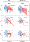 |
Fig. C.1. Comparison between three star formation models (top, middle, and bottom) and PHANGS measurements of the population-average |


As noted previously, the relation between ϵff and σ (rather than Σ or αvir) is our preferred point of reference, as the measurements  and
and  that we compare against are most independent of each other. As emphasized by Leroy et al. 2025, the correlation introduced between measurements of
  and
and  (or ⟨αvir⟩ involving
  ), which are not independent, makes interpreting the relation between these variables less straightforward.
In this illustration, we set the basic model parameters shared by the models (ϵcore = 0.5, b = 0.87, and gas sound speed cs = 0.3 km s−1) to the values used in Figure 1, and select the same critical density scrit given by Eq. 4 for all models. Note, though, that as in Figure 1, the KM05 and FK12 predictions adopt ϕt = 1.9, whereas the sgMFF model adopts ϕt = 1. As noted previously, variations in these basic parameters are not expected to greatly extend the range of the predictions. The addition of the PL in the sgMFF model, on the other hand, gives predictions from this model an added degree of freedom compared to either KM05 or FK12. We opt to show each sgMFF trend line surrounded by a band that represents the rms spread in α around the average trend fit to the measurements in Figure 7 (reported in the text).
The predictions in Figure C.1 exhibit a number of interesting features. First, although the dynamic range of the FK12 model is overall larger (see Figure 1), over the observed range of cloud properties in the PHANGS-ALMA sample under consideration, this model exhibits the least variation in ϵff. The three trend lines do not encompass the observed range in efficiency as well as either the KM05 SFF or the sgMFF model although, in both left and right panels, each trend line sits along the horizontal average near enough to similar-valued measurements.
In comparison, the KM05 model does a better job of spanning the range in  given the observed gas properties. The trend lines sit near the positions of similar-valued measurements in both the horizontal and vertical axes. However, not all of the features of the measurements are reproduced by the predictions. In the middle right panel, for example, regions with low αvir exhibit a wider range in
  than predicted and some of the high αvir regions appear to form stars more efficiently than in the model. In the middle left panel, the KM05 model also falls short of predicting the lowest (highest) efficiencies at low (high) Σ.
As shown in the top row, the sgMFF model performs at least as well as the KM05, starting with a foundation that is more similar to the FK12 model. As discussed in §6.6, elements of both of these models are reproduced by sgMFF, although the addition of the PL yields even greater flexibility to match the observations. Indeed, many of the shortcomings of the KM05 (or FK12) model can be overcome since, by design, the sgMFF model in this instance has been calibrated to reproduce many of the features at fixed Σ and αvir that were not well reproduced by KM05 or FK12. In the left panel, for example, fixed Σ trends capture a wider range of ϵff and now also show a slightly larger decrease in efficiency with increasing Σ that was only modest in KM05 and absent in FK12. In addition, predictions from sgMFF at low αvir in the top right panel are shifted down compared to the KM05 prediction (middle right panel), correcting for the overestimation in ϵff in the KM05 model there.
It should be kept in mind that the model predictions shown here are tailored to apply under the conditions in the gas observed by PHANGS-ALMA. Predictions would vary when applied to high-z objects, for example, which we thus omit from the present comparison. For such cases, the relation between virial state and internal structure is likely different than prescribed by the relation between α vs. αvir calibrated using PHANGs observations of the gas in extragalactic star forming disks. To match the high-z points appearing in Figure 1 with sgMFF model, the PL index α would need to more closely approach 1.5 (see Figure 3), placing the gas in those objects very near a state of pure free-fall collapse. Alternatively, the self-gravitating component would need to appear only at densities above the critical density, so that the core formation efficiency is strongly tied to the LN part of the PDF and boosted as in the original HC11 and FK12 models.
All Tables
All Figures
|
Fig. 1. Time-average ϵff measured in 1.5-kpc-wide hexagonal apertures sampling throughout 67 nearby galaxies targeted by PHANGS, as measured by Leroy et al. (2025). Measurements are plotted against the average cloud-scale velocity dispersion |
| In the text | |
|
Fig. 2. (Left) Predictions for ϵff from turbulence-regulated SF models with a hybrid LN plus PL smooth-PDF proposed by Burkhart (2018) in the SFF (blue) or multi-free-fall (red) scenarios. In these hybrid PDFs, the transition from LN to PL behavior is set to the critical density, st = scrit, as argued by Burkhart & Mocz (2019). A range of PL slopes 1.6 < α < 2.1 set to the range observed by Kainulainen et al. (2014) and Schneider et al. (2022) are indicated by the width of each band. In this example, ϵcore = 0.5, αvir = 5, b = 0.87, and the sound speed cs = 0.3 km s−1. Following Burkhart (2018), we set ϕt = 1. Light gray points show the PHANGS measurements from Leroy et al. (2025), and the dark gray bar and point depict the Dessauges-Zavadsky et al. (2023)z ∼ 1 clumps, repeated from Figure 1. (Right) Illustration of the typical hybrid density PDFs associated with the ϵff predictions in the SFF (blue) and multi-free-fall (red) scenarios at the average cloud-scale velocity dispersion ⟨σc⟩ = 5 km s−1, corresponding to ℳ = 16.7. The blue PDF adopts a PL with slope α = 1.8, which is associated with st = 6.9 (see Eq. (11); marked by the vertical dotted blue line) given the average σc, and yields SFF ϵff predictions such as those shown in blue in the left panel. The red PDF adopts a PL with slope α = 2.7 from the range required to match MFF predictions to the observed ϵff. In this case, the PL starts at st = 11.4 (marked by the vertical dotted red line). Also shown are PDFs with properties matching those measured in local clouds by Schneider et al. (2022). Out of two LNs and two PL components identified by Schneider et al. (2022), only the primary LN and PL components are indicated. These have st = 1 − 2, marked by the narrow vertical gray band, resulting in a kinked appearance. The lighter, wider vertical gray band shows the range in st predicted using Eq. (13) given the observed properties of the plotted regions. |
| In the text | |
|
Fig. 3. (Left) Predictions for ϵff from turbulence-regulated SF models with the hybrid LN+PL PDF proposed here (Eq. (32)) in the SFF (blue) or multi-free-fall (red) scenarios. In these hybrid PDFs, the transition from LN to PL behavior is set to the density threshold for gas to kinematically decouple from the galaxy (Meidt et al. 2020). A range of PL slopes 1.6 < α < 2.1 set to the range observed by Kainulainen et al. (2014) and Schneider et al. (2022) are indicated by the width of each band. As in Figure 2, here we set ϵcore = 0.5, ϕt = 1, αvir = 5, b = 0.87, and cs = 0.3 km s−1, and use the KM05 critical density in Eq. (4). Here we also adopt a fixed γ = 1. Light gray points show the PHANGS measurements from Leroy et al. (2025), and the dark gray bar and point depict the Dessauges-Zavadsky et al. (2023)z ∼ 1 clumps, repeated from Figure 1. (Right) Illustration of typical hybrid LN+PL density PDFs that can fit the observed ϵff. All cases adopt the average cloud-scale velocity dispersion |
| In the text | |
|
Fig. 4. Cloud-scale values of γk = 0 estimated with Eq. (23) shown as a function of galactocentric radius for the subset of hexagonal apertures that sample within galaxies with fitted rotation curves (see Appendix A). Moving inward toward galaxy centers, the influence of the self-gravity of clouds weakens with respect to the galactic potential. |
| In the text | |
|
Fig. 5. Histograms of the PL slope α in the hybrid (LN plus PL) PDFs that match four different SF models (black, blue, red, and dashed red) to the ϵff measured in PHANGS. The fiducial shortened-duration broad-PL MFF model is shown in black, the full-duration broad-PL MFF model is shown in blue, the Burkhart smooth-PDF MFF model is shown in red, and the Burkhart smooth-PDF SFF model is shown in red with a dashed line. |
| In the text | |
|
Fig. 6. Diagnostics of the hybrid LN plus PL density PDFs that match different MFF (and SFF) SF models to the ϵff values measured in PHANGS. From left to right: Slope of the PL component of the PDF α, the dense gas fraction fd measured above a fixed density threshold (see text), and the self-gravitating fraction fsg measured above the critical density scrit. The top row shows results for PDFs in the fiducial broad PL – the shortened duration model given in Eq. (32) – adopting an MFF scenario. The second row shows results for PDFs in the broad PL – full duration model with tobs = tstop in Eq. (32) also in the MFF scenario. The bottom two rows show MFF (third row) or SFF (fourth row) predictions adopting hybrid smooth-PDFs in the Burkhart formulation, with st = scrit advocated by Burkhart & Mocz (2019). All SF models shown here have assumed ϵcore = 0.5, ϕt = 1, b = 0.87, and cs = 0.3 km s−1, and the critical density given in Eq. (4). As indicated by the color bar in the top right panel, points are color-coded by galactocentric radius (increasing outward, from red to purple). The symbol style denotes relative gas surface density; in all radial bins, regions sitting below the 30th percentile are marked with diamonds, regions between the 30th and 70th are marked with a circle, and regions above the 70th percentile are marked with a cross. The gray points in the bottom row repeat the measurements from the top row. The horizontal gray line (band) in the top left panel shows the mean (full spread) of the PL slopes α observed in local clouds (Kainulainen et al. 2014). The gray band in the middle panels illustrates the relation between the dense gas fraction and the gas surface density fit by Neumann et al. (2023). The width of the band represents the full spread in the fitted data (roughly 3 times the scatter about the fit line). |
| In the text | |
|
Fig. 7. Variation in the PL slope α calculated with the shortened duration model given in Eq. (32) as a function of the cloud-scale virial parameter αvir. Symbol shapes and colors are the same as in Figure 6. The horizontal gray line (band) shows the mean (full spread) of the PL slopes α observed in local clouds (Kainulainen et al. 2014). The reference line given by Eq. (35) with ℛα = 0.23 ± 0.06 is shown in black. Combining the systematic variation of dense gas fraction with virial state implied here together with variations in the critical density (depending on αvir) produces SF efficiencies that match the PHANGS observations in Fig. 1 (see also Fig. C.1 and the discussion in Sect. 6.6). |
| In the text | |
|
Fig. C.1. Comparison between three star formation models (top, middle, and bottom) and PHANGS measurements of the population-average |
| In the text | |
Current usage metrics show cumulative count of Article Views (full-text article views including HTML views, PDF and ePub downloads, according to the available data) and Abstracts Views on Vision4Press platform.
Data correspond to usage on the plateform after 2015. The current usage metrics is available 48-96 hours after online publication and is updated daily on week days.
Initial download of the metrics may take a while.