| Issue |
A&A
Volume 700, August 2025
|
|
|---|---|---|
| Article Number | A212 | |
| Number of page(s) | 12 | |
| Section | Stellar structure and evolution | |
| DOI | https://doi.org/10.1051/0004-6361/202553855 | |
| Published online | 26 August 2025 | |
The model fitting of Gaia DR3 classical Cepheid light and radial velocity curves
1
INAF-OACN Osservatorio Astronomico di Capodimonte, Salita Moiariello 16, 80131 Napoli, Italy
2
INAF-Osservatorio Astronomico d’Abruzzo, Via Maggini sn, 64100 Teramo, Italy
3
Istituto Nazionale di Fisica Nucleare, Sezione di Napoli, Complesso Universitario di Monte S. Angelo, Via Cinthia Edificio 6, I-80126 Napoli, Italy
4
European Southern Observatory, Karl-Schwarzschild-Strasse 2, 85748 Garching bei München, Germany
5
Scuola Superiore Meridionale, Largo San Marcellino10, I-80138 Napoli, Italy
⋆ Corresponding author: This email address is being protected from spambots. You need JavaScript enabled to view it.
Received:
22
January
2025
Accepted:
19
June
2025
Abstract
Context. Classical Cepheids are fundamental astrophysical laboratories for studying stellar structure and evolution, as well as for calibrating the cosmic distance scale. Despite significant progress in observational and theoretical studies, uncertainties remain regarding their masses, luminosities, and distances, as well as the role of processes such as core overshooting, rotation, and mass loss. The advent of high-precision data from Eurepan Space Agency (ESA) Gaia’s Data Release 3 (DR3) provides an opportunity to address these questions.
Aims. The primary aim of this study is to estimate the main structural parameters and distances of a sample of classical Cepheids using non-linear convective pulsational models. The work also seeks to test the consistency of Gaia parallaxes, independently constrain the mass–luminosity (ML) relation, and investigate the dependence of the projection factor (p-factor) on the pulsational period.
Methods. A sample of 46 classical Cepheids with precise photometric and radial velocity data from Gaia DR3 was analysed. Model fitting was conducted by directly comparing predicted and observed variations in GaiaG , GBP, and GRP light curves, as well as radial velocity time series. Distances inferred from the models were compared to Gaia parallaxes, including corrections provided by the Gaia team. Predicted masses and luminosities were used to constrain the ML relation, while the inclusion of radial velocity curves allowed for an independent estimation of the p-factor.
Resuts. The comparison between inferred distances and Gaia parallaxes reveals a statistical agreement, indicating no need foradditional global offset corrections. The predicted masses and luminosities are consistent with an evolutionary scenario that includes a small or mild amount of core overshooting, mass loss, or rotation. Our analysis of the p-factor does not suggest a significant period dependence, with a constant value of p = 1.22 ° 0.05 , which is consistent with recent literature. Additionally, our results align well with the recent period–Wesenheit–metallicity relation derived from Gaia DR3 photometric magnitudes combined with parallax measurements.
Key words: stars: distances / stars: fundamental parameters / stars: oscillations / stars: variables: Cepheids / distance scale
© The Authors 2025
 Open Access article, published by EDP Sciences, under the terms of the Creative Commons Attribution License (https://creativecommons.org/licenses/by/4.0), which permits unrestricted use, distribution, and reproduction in any medium, provided the original work is properly cited.
This article is published in open access under the Subscribe to Open model. This email address is being protected from spambots. You need JavaScript enabled to view it. to support open access publication.
1. Introduction
Classical Cepheids (CCs) are the most important primary distance indicators when calibrating the cosmic distance scale. The physical basis of the existence of period–luminosity (PL) and period–luminosity–colour (PLC) relations for these stars is well known. The existence of a period–luminosity–temperature–mass (PTLM) relation directly descends from the period–mean density relation and the Stefan-Boltzmann law (see e.g. Bono et al. 1999; Marconi et al. 2013a, and references therein). Moreover, it is well known from stellar evolution models that intermediate-mass stars, depending on their chemical composition, obey a mass–luminosity (ML) relation, during their central He-burning phase (see e.g. Chiosi et al. 1992, 1993; Bono et al. 1999). According to several authors (see e.g. Chiosi et al. 1993; Bono et al. 1999; Anderson et al. 2014, 2016, and references therein), the presence of non-canonical effects (e.g. core overshooting, mass loss, and rotation) results in a systematic increase in the luminosity obtained from the ‘canonical’ ML relation. For example, De Somma et al. (2020, 2022) considered two over-luminosity levels above the canonical relation (+0.2 dex and +0.4 dex) to take non-canonical effects into account. By combining the PTLM with the ML relation, one obtains aperiod–luminosity–temperature (PLT) or PLC relation. The widely adopted PL relations result from the projection of the PLC relation onto a PL plane (see Madore & Freedman 1991), which implies neglecting the finite colour extension of the instability strip. Another relation, the so-called period–Wesenheit (PW) relation (Madore 1982), is obtained by replacing the magnitude with a function defined as the magnitude corrected for a colour term, multiplied by a coefficient that is exactly the ratio between the total and the selective extinction. This function is reddening-free by definition, provided that an extinction law is assumed a priori. Thus, the coefficients of the ML relation affect the PL, PLC, and PW relations and, in turn, the Cepheid distance scale. In this context, a combination of accurate geometric distance information and independent pulsation modelling results is needed to constrain the ML relation. The third ESA Gaia Data Release (Gaia DR3) includes a sample of 799 Cepheids and 1096 RR Lyrae (see e.g. Katz et al. 2023; Clementini et al. 2023; Ripepi et al. 2023, and references therein) with parallaxes, epoch photometry, and radial velocity (RV) measurements. The adopted dataset is the fundamental basis forinvestigating Cepheid stellar parameters.
From a theoretical point of view, the use of non-linear convective pulsation models to compare predicted and observed light and RV curves represents a powerful tool for simultaneously constraining the intrinsic stellar parameters and the individual distances of the investigated pulsating stars. Several applications in the literature support the predictive capabilities of this method for both the CCs (see e.g. Wood et al. 1997; Bono et al. 2002; Keller & Wood 2002, 2006; Natale et al. 2008; Marconi et al. 2013a,b, 2017; Ragosta et al. 2019) and RR Lyrae (see e.g. Bono et al. 2000a; Marconi & Clementini 2005; Marconi & Degl’innocenti 2007).
These pulsation codes are not only capable of predicting stellar parameters, but they also have been able to describe dynamical phenomena of these stars, for example beat Cepheids (Kolláth et al. 2002), double mode RR Lyrae behaviour (Szabó et al. 2004), and period doubling and related non-linear phenomena (Kolláth et al. 2011; Plachy & Kolláth 2013; Smolec 2014, 2016). Meanwhile, PL relations have been extensively studied as well (see e.g. Marconi et al. 2015, 2018; Deka et al. 2022; Das et al. 2021, 2024)
In this work we used a new extensive set of non-linear convective pulsation models to fit a subsample of 46 fundamental CCs from the Gaia DR3 dataset. This represents the largest sample of CCs analysed so far through the model fitting technique.
The work is structured as follows: In Sect. 2 we present the adopted sample, and the new computed pulsation models are discussed in Sect. 3. The developed model-fitting approach is outlined in Sect. 4, together with the selection of the best-fit models based on the inclusion of Monte Carlo simulations. Section 6 presents the results of the fitting method, and Sect. 7 some closing remarks.
2. The sample selection
The initially adopted sample of sources was obtained from a query to the Gaia public archive1. All the DR3 fundamental mode CCs, all of which have epoch RV data were extracted and amounted to 799 variables. This catalogue was cross-matched with the list of confirmed Galactic CCs by Ripepi et al. (2023). This cross-match left us with 558 variables. Since the pulsational model calculation is very time-consuming, we decided to reduce the sample by selecting only those having a good phase sampling in the RV curve2. To this aim, we modelled the RV time series by fitting them with a truncated Fourier series (Appendix A) and selected only those without large and/or spurious model oscillations, possibly due to wide phase intervals with a dearth of measures. In particular, a selection was performed considering only sources according to the following conditions: (i) RV curves with at least 20 data points; (ii) a uniformity index3UIRV > 0.9; (iii) visual inspection to remove the remaining few bad sources; and (iv) DR3 relative parallax error σϖ/ϖ < 50%.
After this procedure, the sample was reduced to 198 selected sources. This sample was further reduced by looking at the residuals around the Fourier models, for both photometric and RV data. Specifically, we performed a statistical analysis of the Fourier fit scatter for all time series. In particular, we calculated the root mean square (rms) of residuals around the Fourier model for all the considered photometric and RV curves and removed all the sources with the rms of residuals deviating by more than 3.5 median absolute deviations (MADs) from the median of the rms distribution, for one or more observed time series. The remaining sample after this step contains 46 sources.
We then complemented the information with available metal abundance measurements, as metallicity is a key parameter affecting stellar pulsation and the shape of the light and RV variations. We adopted the work by Trentin et al. (2024, T24), which reports the iron abundance for more than 900 CCs obtained based on high-resolution spectroscopy.
The period and the [Fe/H] distributions of our final sample are shown respectively in Figs. 1 and 2, while Fig. 3 shows the distribution of Z values, obtained4 by assuming the elemental composition of the Sun Z⊙ = 0.02 dex (see e.g. Buldgen et al. 2024, and references therein)
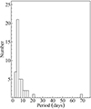 |
Fig. 1. Distribution of the selected classical Cepheids period values obtained from the DR3. |
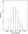 |
Fig. 2. Distribution of the selected classical Cepheids [Fe/H] values obtained through high-resolution spectroscopy (T24). |
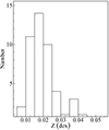 |
Fig. 3. Distribution of the Z values of all the selected variables computed by converting the spectroscopic [Fe/H] values from Trentin et al. (2024). |
3. Pulsational model computations
The theoretical framework considered in this work is based on a non-linear radial pulsation code that adopts a non-local time-dependent treatment of the turbulent convection (see e.g. Stellingwerf 1982; Bono & Stellingwerf 1994; Bono et al. 1999, and references therein).
The procedure followed to obtain the hydrodynamic pulsational models reproducing the observed light and RV curves, consists of four main steps: (i) the definition of a multi-dimensional grid of possible structural parameter (M , Teff , log(L/L⊙) , α 5) values to be given as input to the hydrodynamical code to reproduce the observed period; (ii) the linear analysis that provides the static envelope structure to be perturbed through the subsequent non-linear analysis; (iii) the non-linear analysis aiming at producing the final full-amplitude pulsating models, including both absolute bolometric magnitude and pulsational velocity curves; and (iv) the transformation of the theoretical bolometric light curves into the Gaia photometric system.
3.1. Initial grid of structural parameters
Since chemical composition plays a key role in the computation of pulsation models, and given that the selected sample spans a wide range in Z, from Z < 0.01 dex to Z ≃ 0.045 , we decided to divide the sample into four metallicity bins centred around the values Z1 = 0.01 dex, Z2 = 0.02 dex, Z3 = 0.03 dex, and Z4 = 0.04 dex, each characterized by a width of 0.005 dex. The helium contents (Y), corresponding to the adopted Z bins, are Y1 = 0.26 , Y2 = 0.28 , Y3 = 0.28, and Y4 = 0.29 dex. Based on this division, each bin contains 13, 24, 5, and 4 sources, respectively. From this point forwards, the central value of each bin will be representative of the elemental composition of the stars within that bin.
For each fixed chemical composition, the input mass and effective temperature values for the linear analysis were varied on a rectangular grid, covering the ranges  with a step of 0.5 M⊙ and
  with a step of 50 K. Then, for each combination of mass and effective temperature, the luminosity value is found by satisfying the observed period, as described in Appendix B. In this procedure only luminosities satisfying a variation within −0.06 dex to 0.6 dex with respect to the canonical ML relation, as predicted by Bono et al. (2000b), are kept for the following analysis (see Appendix B). The lower limit corresponds to –3 times the standard deviation of the adopted ML relation (Bono et al. 2000b), while the upper limit takes into account the presence of full core overshoot (Chiosi et al. 1993). Taking advantage of the well-known relations between luminosity and the other structural parameters, our method allows us to define a complete grid of initial structural parameters, by significantly reducing the number of models to be computed.
As regards to the α parameter, it was varied between 1.4 and 1.9 in steps of 0.05, resulting in 11 possible α values. We note that when the α values do not match those provided in Table 3 of De Somma et al. (2020), we applied linear interpolation if our values fell between two of those considered by the authors, or we adopted their most extreme relations if our values lay outside their specified α range.
3.2. The hydrodynamical analysis
The linear survey is based on a non-adiabatic radiative code (see Bono et al. 1999, and references therein, for detail) that was run for all the M–Teff –log(L/L⊙) values defined above for each assumed chemical composition. The subsequent non-linear analysis takes the static structure and the predicted eigenfunctions obtained from the linear code as input and enables the determination of which models exhibit a full amplitude stable pulsational behaviour.
The non-linear code introduces an initial dynamical perturbation (typically 20 km/sec) to the static model, modulated within the envelope structure with the predicted radial eigenfunction obtained from the linear analysis. Subsequently, it monitors the time evolution of its characteristic parameters to assess the attainment of full amplitude behaviour. Integration of hydrodynamical equations is performed over a considerable number of periods, with the satisfaction of convergence conditionsdetermined by the total work approaching vanishing values and the peak-to-peak bolometric amplitude exhibiting negligible change (see below).
Typically, the code is initiated with a fixed number of computing cycles, ranging from 1000 to around 10 000, depending on the model’s mass and position within the instability strip, with models located close to the extreme edges of the strip typically requiring a larger number of cycles. Given the resource-intensive nature of the non-linear step, we implemented runtime tests within the code to assess the model’s convergence status. Specifically, the non-linear code computation is halted under the following circumstances over the last 40 period cycles:
(i) The normalized total work remains stable around vanishing values (≤5 ⋅ 10−4), and the peak-to-peak bolometric magnitude amplitude shows minimal variation, staying below 5 ⋅ 10−3 mag.
(ii) The peak-to-peak amplitude is consistently smaller than 0.02 mag and steadily decreasing.
(iii) The conditions described in point (i) are met, but the period converges to the expected value associated with another pulsation mode (the model reaches a stable pulsational regime but with a mode that is not the required one).
Upon meeting the conditions in point (i), the model achieves full amplitude behaviour, pulsating stably. Conversely, if conditions (ii) or (iii) are satisfied, the pulsation ceases or the model switches to a different pulsational mode. This strategy allowed us to speed up the model computation by stopping it before the assumed total number of cycles is reached, as soon as the convergence condition is achieved, and in particular when the pulsation behaviour switches off or changes mode.
3.3. Converting from bolometric to Gaia multi-filter light curves
The conversion of the bolometric magnitude curves into the Gaia photometric bands was achieved by adopting the bolometric correction grids based on the PHOENIX model atmosphere (Chen et al. 2019). We refer the reader to Marconi et al. (2021) for all the details of our adopted procedure. Here we just recall that we used a proprietary C code to interpolate the Chen et al. (2019) tables to obtain the bolometric corrections corresponding to the log(g) , Teff, and Z of our modelled curves. For all the transformed models we assumed  mag (De Somma et al. 2022, and references therein).
4. The model fitting method
The adopted model fitting procedure is based on the minimization of the following χ2 functions (see also Marconi et al. 2013a, 2017; Ragosta et al. 2019):
 (1)
(1)
 (2)
(2)
where we included the term χAmp2 for every fitted band (including RVs), which is equal to
 (3)
(3)
To justify the inclusion of this additional term, we performed tests that revealed that, in some cases, models minimizing the χ2 function without the  term, do not always reproduce the peak-to-peak amplitude of the observational curves. We therefore decided to give greater weight to models that also reproduce as good as possible the amplitude, whose reference value (AmpFourierj) is derived from the Fourier model constructed as previously described.
The first equation above refers to the j-th photometric band, while the second equation is used to fit the RV curve. The sums are performed over the number of observational data points for both photometry (Npts) and RV (Mpts). The lower case symbols, ϕ, m, and v indicate the pulsation phases, the measured magnitude, and the measured RV, respectively. The upper case functions Mj(ϕ) and Vpuls(ϕ) give analytic expressions for the model j-th photometric band and the pulsational velocity curves6. The expected outputs of this best-fitting procedure are the distance modulus, μj, and the phase shift,  , in the j-th band for the photometry, while the model fitting of the RV curves provides information on the projection factor,
  , the velocity of the centre of mass, γ, and the phase shift,
  .
.
The projection factor (p-factor) allows us to compare the modelled pulsational velocity to spectroscopically measured RV. It quantifies the projection of the pulsational velocity of the stellar atmosphere along the line of sight. In particular it is defined as p = Vpuls/RV and assumes values larger than 1.0. The value of the p-factor is debated in the literature due to the difficulty of its determination. Indeed, it depends on the physical structure of the stellar atmosphere, on the velocity gradient in the atmosphere and on the way the RV is obtained experimentally (see e.g. Nardetto et al. 2011; Molinaro et al. 2011; Ragosta et al. 2019, and references therein). The first works addressing the problem of the p-factor from a theoretical perspective date back to Eddington (1926) and Carroll (1928). These authors, by including the effects of limb darkening and constant-velocity expansion of the stellar atmosphere in their theoretical models, obtained a p-factor value of p = 24/17 = 1.41. This value is close to the maximum limit, 1.5, which is derived when the Cepheid is approximated as a simple uniform disk (Nardetto 2017). A more complex model, which accounts not only for the geometric effect but also for the relationship between the stellar surface’s RV and that derived from spectral lines, was developed for example by Nardetto et al. (2004). This model also includes the effects of limb darkening and atmospheric velocity gradients. Several studies have investigated the existence of a relationship between the p-factor and the pulsation period, but no definitive conclusion has been reached so far (Groenewegen 2007, 2013; Kervella et al. 2017; Nardetto et al. 2009; Neilson et al. 2012; Storm et al. 2011).
In the current work, we forced the p-factor values to be in the range 1.10–1.5 to take current uncertainties in the literature evaluations into account. The upper limit was fixed according to the expected maximum theoretical value, as stated above, while the lower limit was adopted according to the recent results obtained by Trahin et al. (2021). They calibrated the p-factor value by combining the parallax-of-pulsation method, implemented through the SPIPS algorithm (Mérand et al. 2015), with the Gaia Early Data Release 3 (EDR3) parallaxes (see also Anderson et al. 2024; Breitfelder et al. 2016; Trahin et al. 2021). Finally the fitted phase shifts are introduced to take into account small uncertainties in the estimate of the phases of the observations, and are typically around ∼0.02.
In the current work, the χ2 minimum value was obtained using an analytical approach, rather than relying on commonly used numerical minimization routines (e.g. Levenberg 1944). Specifically, we show that minimizing the χ2 function in Eqs. (1) and (2) can be reduced to solving two equations for the unknowns δΦj and δΦRV, while the remaining fit parameters can be expressed as functions of these phase shifts (see Appendix C). This approach was feasible in our specific case because we were able to derive the first-order analytical derivatives and solve the resulting system of equations explicitly.
The minimization procedure is applied separately to each photometric band and to RV, and finally, the obtained minimum χ2 values are combined into one cumulative minimum value according to the following relation:
 (4)
(4)
where Nbands is the number of available bands (including RV), while (d.o.f)j represents the number of degrees of freedom for the j-th band7.
Here we want to focus the attention on the fact that Eq. (4) was minimized at fixed α value, for all the possible values we used to divide the range 1.4–1.9 (see Sect. 3.1). Finally, the optimal α value was determined as described below. For each candidate  , we: selected the corresponding subsample of pulsation models; performed independent fits by minimizing the
  function (Eq. (4)); recorded the resulting best-fit
  value; and chose the final α such that it satisfies
  .
.
5. Monte Carlo methods for best model selection and uncertainty quantification
Monte Carlo techniques encompass a broad class of numerical methods based on the random resampling of a dataset to derive statistical estimates (e.g. confidence intervals and error estimations). In this work we used two different kinds of simulations: (i) bootstrap simulations, obtained by resampling input time series; and (ii) Monte Carlo simulations with observational noise injection. The following subsections detail each method’s implementation and their specific roles in our analysis.
5.1. Bootstrap resampling
Among Monte-Carlo simulations, bootstrap resampling is a widely used approach. Bootstrap methods come in several variants (e.g. parametric, non-parametric, and jackknife), and we refer the reader to the review by Feigelson & Babu (2012) for a comprehensive discussion. In this study, we specifically applied the classical non-parametric bootstrap method. This approach involves generating mock datasets by randomly resampling the original dataset with replacement. Each simulated dataset has the same size as the original set of measurements, but individual data points can appear multiple times, while others may be absent in a given resampled dataset (Feigelson & Babu 2012).
In our work, we performed 250 random simulations. This number was chosen to strike a balance between computational time and the need for a sufficiently large number of trials. Each random experiment consists of two main steps:
-
Resampling: The observational time series of both photometry and RV are resampled with replacement, ensuring that each mock dataset retains the same number of data points as the original one.
-
Model fitting: The full fitting procedure is repeated for each mock dataset.
This approach serves a dual purpose. First, for a given n-tuple of structural parameters (M, Teff, log L/L⊙)8, corresponding to a fixed stellar model, the simulations allow us to quantify the uncertainties in the fitted parameters derived from the solutions of Eqs. (C.1), (C.2), (C.3), (C.4), and (C.5) (namely μi, ϕi, γ, ϕrv, and the p-factor). The uncertainty for each fitted parameter is computed as the robust standard deviation (1.4826 · MAD), which rescales the MAD to match the standard deviation of a normal distribution. These values are obtained from the 250 best-fit solutions generated by the Monte Carlo realizations.
Second, for each of the 250 simulations, the optimal pulsation model is identified as the one minimizing the total χ2 function defined in Eq. (4). This yields a distribution of optimal models that typically span multiple nodes of the parameter-space grid. Since the location of the minimum χ2 varies from simulation to simulation, this dispersion provides a direct measure of the parameter-space degeneracies introduced by observational uncertainties. This behaviour is a fundamental property of χ2: if the phase coverage of the data is uneven, the best-covered phases will dominate the χ2 statistic, effectively weighting those regions more heavily during minimization. Our resampling strategy, combined with the inclusion of the peak-to-peak amplitude term (Eq. (3)), helps mitigate this effect.
Focusing on the last itemized point discussed above, we analysed the distribution of minimum χ2 values (hereafter χmin2) obtained from our 250 simulations. A statistical characterization of this distribution enabled us to estimate the expected minimum χ2 value. We adopted the median as a robust central estimator, and the 5th–95th percentile range as a measure of its uncertainty. Prior to this analysis, significant outliers – defined as values beyond ±3.5 ⋅ MAD – were excluded to ensure statistical reliability. All models contributing to the clipped χmin2 distribution were then used to infer the optimal structural parameters and their associated uncertainties. This subset defines the best-fitting solutions for the observed source. For each structural parameter (mass, Teff, and log(L/L⊙)), the best estimate was taken as the median of its distribution, while the uncertainty was quantified via the semi-range (i.e. half the difference between the maximum and minimum values). This conservative approach was adopted to: (i) provide a robust estimate that reflects the full variability of viable solutions; (ii) avoid assumptions regarding the shape of the underlying distributions; and (iii) prevent the underestimation of the true uncertainties.
5.2. Measurement-error-driven Monte Carlo sampling
In addition to the bootstrap technique introduced in the previous section, this work employs another Monte Carlo-based approach. Specifically, to estimate the uncertainty associated with a given property in our sample of Cepheids – and to perform a statistical analysis that incorporates the measurement errors affecting each input data point (e.g. the p-factor and global parallax offset) – we adopted the following methodology: (i) we conducted 250 Monte Carlo simulations, perturbing each data point within its error bar under the assumption of Gaussian noise statistics, and (ii) for each realization, we computed the mean of the studied quantity. The resulting distribution of the 250 mean values was then analysed, and we defined the 5th-95th percentile interval as the best estimate of the uncertainty for the considered quantity.
6. Results of the fit
The multi-filter Gaia light curves and the velocity curves of the best models found (lines) for all the selected sources, are shown in Fig. D.1, over-imposed to the observed photometric and RV time series. Table D.1 lists the best-fit parameters derived from our analysis. For each star, we report the optimal estimate of the pulsation period (Pbest), the corresponding value of the α parameter, and the central values of metallicity and helium content (Zbest, Ybest) characterizing the best-fitting chemical composition bin. We also provide the best-fit structural parameters, namely mass (M), effective temperature (Teff ), and luminosity (log(L/L⊙)), as well as the over-luminosity (ΔML) with respect to the canonical ML relation. Additionally, the table includes the best-fit p-factor, the γ velocity, the theoretical parallax estimate, and the global χ2 value obtained by minimizing Eq. (4)
While not perfect, the theoretical framework provides a reasonable match to both light and RV curves, demonstrating its ability to predict multi-filter variations of Cepheids with different periods and metallicities, despite some systematic deviations. Here we list the main features and issues around the fit, hinting that the problem of stellar pulsation is still not solved:
-
Systematic larger modelled amplitudes in the photometric Gaia bands than in the RV curves (CK Cam, V407 Cas, IN Aur, V432 Ori, OZ Cas, V737 Cen, and S Vul): These discrepancies could potentially be reduced by fine-tuning the α parameter, as increasing α might yield models with smaller photometric amplitudes, thereby improving the fit. However, raising α would also decrease the p-factor (see Eq. (2)), which – especially for stars like IN Aur, V432 Ori, OZ Cas, V737 Cen, and S Vul – could push it towards the lower limit of the physically expected range. The observed differences likely stem from limitations in the current treatment of convection-pulsation coupling, particularly the challenges associated with turbulent convection modelling (Marconi et al. 2017; Kovács et al. 2023).
-
Minor phase shifts in secondary features (BF Cas, V384 CMa, AP Pup, WX Pup, and OGLE-GD-CEP-0339): These small discrepancies can rise from limitation in the treatment of the convection-pulsation coupling that affects the relative amplitude and position of the primary and secondary maximum.
-
Severe mismatches (V339 Cen, HZ Per, SS CMa, AD Pup, RZ Vel, and S Vul): The point detailed above is more evident in these cases, which are closer to the red edge of the instability strip and in some cases affected by limitations in the light curve sampling (see e.g. S Vul).
All the cases listed are characterized by a global χ2 value significantly exceeding the expected value of 1, reflecting notable discrepancies between the model and the observations. While these issues are essential to resolve for a complete understanding of the underlying physics, they have a minor impact on the determination of structural parameters. In the following sections, we therefore focus on presenting the results from the analysis of the best-fit model properties.
6.1. Predicted versus measured periods
In Fig. 4 we compare the pulsational periods based on the best-fit models, with the values from Gaia DR3. In the bottom panel we show the percentage differences between modelled periods and observational periods. The median and the robust standard deviation (1.4826 · MAD) of the differences are 1.3% and 1.6%, respectively, while the maximum and minimum differences do not exceed 10%.
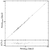 |
Fig. 4. Top panel: Modelled period values (vertical axis) versus the DR3 periods (horizontal axis). The 1:1 line is also plotted to facilitate the comparison. Bottom panel: Percentage difference between the theoretical periods and the DR3 values as a function of the observational period. |
6.2. The projection factor
As previously noted, the match between the theoretical and observed amplitudes of the RV curves provides the corresponding stellar p-factor.
Using the inferred results for the p-factor, we investigated its trend with the period by fitting the equation  . The results of this analysis are shown in Fig. 5. In the figure, we have highlighted the three different types of fits that were tested. Despite of the fact that the obtained slopes are significantly different from zero, the very small determination coefficient R2 ∼ 0.22 indicates that the correlation is very weak. Although our analysis does not reveal a statistically significant correlation, large uncertainties associated with several p-factor estimates may hinder the detection of a possible underlying trend.
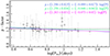 |
Fig. 5. p-factor as a function of the best-fit pulsational period. Three kinds of linear fits are also reported: the weighted linear fit (blue line), the unweighted linear fit (green line), and the robust linear fit (magenta line). The dashed black line indicates the median p-factor computed by considering the whole sample. |
Neglecting the period dependence, we derived the mean p-factor value based on the discussed model fitting results with its associated statistical error: p = 1.22 ± 0.05. The uncertainty on the p-factor was determined through a set of Monte Carlo simulations. First, we varied the p-factor of each individual source within its error, assuming a Gaussian distribution. For eachsimulation, we calculated the mean of the resulting p-factors. Finally, the uncertainty was computed as the 5–95 percentile interval of all the mean values obtained.
The lack of a significant dependence of the p-factor on the pulsation period is consistent with the findings of Nardetto et al. (2009) and Neilson et al. (2012), where the p-factor was calibrated using theoretical models. Similarly, Groenewegen (2007) found no significant period dependence, deriving a constant value of p = 1.27 ± 0.05 by applying the Baade-Wesselink method in its surface brightness form. A comparable p-factor of 1.27 ± 0.06 was also obtained by Mérand et al. (2015) for δ Cep.
Our estimate of the p-factor is in excellent agreement with the values derived for the binary Cepheid OGLE-LMC-CEP-0227 by Marconi et al. (2013a, p = 1.20 ± 0.08) and Pilecki et al. (2013, p = 1.21 ± 0.03 ± 0.04). This binary Cepheid is particularly significant for studying the structural parameters of Cepheids, as its binary nature provides an independent estimate of the primary characteristics of the variable. In Marconi et al. (2013a), the variable was modelled using hydrodynamic pulsation models, while Pilecki et al. (2013) introduced a method specifically designed for analysing double-lined eclipsing binaries containing a radially pulsating star.
Our best estimate is close to the lower end of the assumed p-factor range, but we need to extend the sample in order to equally populate the various period ranges in order to provide more stringent results.
6.3. The α parameter
The determination of p-factor is strongly affected by the choice of the optimal α parameter. Turbulent convection models based on a single-equation formalism, commonly used in radial pulsation studies, often fail to simultaneously reproduce both the RV and photometric variations when a constant p-factor is assumed, as shown by Kovács et al. (2023). This limitation also affects our hydrodynamic code and has similarly been observed in Cepheid models by Marconi (2017).
We notice that, on the basis of our results, no clear trend is found for the variation of α with the effective temperature. However, the sample analysed here might be not large enough to investigate such a dependence, and the large scatter visible in the α versus Teff plot (see Fig. 6) prevents us from drawing firm conclusions. Moreover, metallicity affects the predicted amplitudes and in turn the selected α values, so that differences in metallicity in some cases contribute to the plot dispersion. It is nevertheless interesting to note that, previous findings in the literature, noted an anti-correlation between the eddy viscosity and the effective temperature for RR Lyrae stars by Kovács et al. (2023, 2024). Similar results were reported for classical and type-II Cepheids by Deka et al. (2024), although without an in-depth analysis of this aspect. While one could argue that those previous results were obtained using different codes – namely the Budapest-Florida Code (Yecko et al. 1998) and MESA-RSP (Paxton et al. 2019; Smolec & Moskalik 2008) – similar trends were also found for RR Lyrae stars and bump Cepheids with the Stellingwerf code (Di Criscienzo et al. 2004; Bono et al. 2002). However, all the investigations adopted a single chemical composition and did not simultaneously take photometric and RV variations into account.
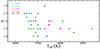 |
Fig. 6. Best-fit α parameter plotted against the best values of the Teff. Different colours indicate different metallicity bins. |
6.4. Absorption
To obtain the reddening-free distance modulus μ0, we corrected the distance moduli in the individual bands (μj parameter in Eq. 1) using the Cardelli extinction law (Cardelli et al. 1989) and the E(B-V) values published in T24. Specifically, we adopted the following equations,
 (5)
(5)
 (6)
(6)
 (7)
(7)
to correct the distance moduli μGBP, μG and μGRP, obtained from the fitting procedure, and finally, we computed the weighted average of the three values, which we consider as our best estimate of μ0.
6.5. Parallax comparison
The reddening free distance moduli, obtained as stated in the previous section, are converted into parallax values (see Col. 14 of Table D.1) and are compared with the Gaia DR3 parallax values (including the correction by Lindegren et al. (2021), hereinafter L21) in Figure 7.
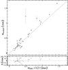 |
Fig. 7. Top panel: Comparison between the Gaia DR3 parallaxes, corrected according to the L21 recipe, and those obtained from our pulsation model fitting technique, shown together with 1:1 line (grey solid). Bottom panel: Residuals, |

The analysis presented in the figure indicates that, for parallax values below approximately 0.50 mas, the individual data points show good agreement with the 1:1 line. For parallaxes above this threshold, however, our fitting procedure tends to yield slightly larger values compared to those from DR3+L21. A similar underestimation of parallaxes was reported by Breuval et al. (2020) based on Gaia DR2 data. While the two results are not directly comparable due to differences between DR2 and DR3, the observed behaviour may suggest thepersistence of residual systematics at higher parallax values. According to our results, we find an increasing agreement between the two parallax samples as the parallax value decreases.
To quantify the offset in the Gaia DR3 + L21 parallaxes, we performed a statistical analysis using the theoretical parallaxes as a reference. This analysis involved a series of Monte Carlo simulations similar to those described in Sect. 6.2.
First, the differences (Δ) between the theoretical parallaxes and those from DR3 were computed. The uncertainty on each Δ value was determined as the quadrature sum of the uncertainties on the theoretical parallaxes and those on the DR3+L21 parallaxes. Monte Carlo simulations were then carried out by perturbing the Δ values within their uncertainties, assumed to follow a Gaussian distribution.
The global parallax offset derived from this analysis is 0.014 mas, with the uncertainty determined using the 5–95% quantile range. These findings suggest that no significant offset exists in the DR3+L21 parallaxes. A comparable result is obtained by calculating the weighted mean and its associated error from the simulations instead of relying on quantile analysis. In this case, the global parallax offset is 0.005 ± 0.012 mas, further supporting the conclusion that the L21 correction improves the agreement between the Gaia DR3 parallaxes and the reference values.
Other authors have derived the global offset in the DR3+L21 parallaxes. Using eclipsing binaries as reference for distance, Stassun & Torres (2021) obtained a positive parallax offset equal to +0.015 ± 0.018 mas, even if even if consistent with zero, in agreement with our findings.
Wang et al. (2022) used a sample of giant stars with accurate known distance and found that the official L21 model largely improves the parallax determination, with a residualoffset amounting to +0.0026 mas, (+0.0029 mas) for the five-parameter (six-parameter) solutions. Fabricius et al. (2021) compared the EDR3 parallaxes with the distances obtained from other external catalogues (see their Table 1) and found that the L21 correction significantly improves the parallax comparison, in agreement with our results.Significant negative global offset values were found by other authors in the sense that L21 recipe seems to over-correct the parallaxes, returning parallaxes larger than the reference values. For instance, Riess et al. (2021) find a global offset Δϖ= − 0.014 ± 0.006 mas, while two other recent studies, Molinaro et al. (2023) and Bhardwaj et al. (2021), found offsets Δϖ= − 0.022 ± 0.004 mas and Δϖ= − 0.022 ± 0.002 mas, respectively. We refer the reader to Fig. 10 in Molinaro et al. (2023) for a more complete review of the most recent determinations of the global parallax offset.
6.6. Period–Wesenheit–metallicity relation
To minimize the effect of reddening on the distance determination, the reddening-free by definition PW relations and their metal-dependent versions (PWZ) are often adopted (see e.g. T24). The period and metallicity values characterizing the investigated Cepheid sample are not representative of the entire expected range for CCs. As a consequence, we did not fit the PWZ relation by using the mean parameters of the selected variables, but we studied how they distribute in comparison with the PWZ relation recently obtained by our group within the C-MetaLL project (see e.g Ripepi et al. 2021; Trentin et al. 2024).
To this end, we calculated the absolute mean Wesenheit magnitude9 in the Gaia bands using the parallax corrections from L21 and the mean magnitudes G, GBP, and GRP from the sample of CCs by T24. The obtained values were plotted as a function of period in the top panel of Fig. 8, by adopting a colour scale showing the trend of the [FeH] values. The data representing our sample are also displayed with magenta circles. Additionally, the best-fit PWZ relation from T24 (see their Table 3) is plotted as a dashed black line. The residuals of our sample relative to the best-fit relation are shown in the bottom panel of the same figure. The agreement appears very good. A statistical analysis hints that there is a marginal systematic residual with median value equal to 0.016 mag, compared with the fitted line. Moreover, the robust standard deviation of the distribution of the residuals amounts to 0.10 mag, indicating that our sample is reasonably distributed around the PWZ relation by T24.
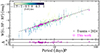 |
Fig. 8. Absolute Wesenheit magnitude plotted against the pulsation period. The fundamental CCs from T24 are also plotted and coloured according to their [FeH] values, together with their best PWZ fitted relation (dashed line). The same quantities for the sample studied in this work are also plotted, together with their errors, with magenta circles. Their residuals around the plotted fit are also shown in the bottom panel. |
6.7. Mass–luminosity relation
The inferred individual mass and luminosity values allow us to understand how the best-fit models compare with the ML relations predicted by stellar evolution. In Fig. 9 we show the distribution of the obtained best-fit models (violet circles), divided into the four selected metallicity bins, in the ML plane, compared with the relations predicted by the adopted stellar evolution scenario in the canonical assumption (black solid line), including a mild (+0.2 dex, red dashed line) or full (+0.4 dex, blue dashed line) over-luminosity due to overshooting or mass loss, or rotation. We notice that for each metallicity bin, the bulk of the model results are located within the canonical and the mildly noncanonical relations, with a smaller number of models between the mildly and the fully non-canonical lines. The inferred dispersion supports the idea that the observed Cepheid sample do not obey a unique universal ML relation, possibly reflecting the stochastic nature of mass loss, thus displaying a non-negligible spread in the ML plane. This dispersion is also expected to affect the coefficients of the PL, PLC, and PW relations.
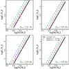 |
Fig. 9. Mass and luminosity best values obtained by our pulsation model fit technique for all the selected sources (violet points), together with the expected canonical ML relation (solid black line), the mild (+0.2 dex) non-canonical ML relation (dashed red line), and the full (+0.4 dex) non-canonical ML relation (dashed blue line). |
7. Conclusions
In this work we used hydrodynamic pulsation models to fit a sample of Galactic CCs for which photometry, RV, and parallax data from Gaia DR3 were available; this was complemented with recent high-resolution spectroscopic metallicities. Several criteria were considered for the sample selection: (i) the widest possible coverage of the expected period range for CCs; (ii) well-sampled light and RV curves in phase; (iii) sufficiently accurate parallaxes (σϖ/ϖ < 50%); and (iv) metallicities obtained through recent high-resolution spectroscopic measurements.
Using the models generated by our hydrodynamic pulsation code, we performed a fitting procedure based on the minimization of the χ2 function. By employing a set of bootstrap Monte Carlo simulations, we investigated how the best-fit model varied by randomly resampling the input data. This procedure allowed us to determine the uncertainties on both the fit parameters and the structural parameters estimated for each variable.
The main results of this best-fitting method are:
-
The pulsational periods are accurately reproduced by hydrodynamical models, with percentage differences that are not larger than 10%.
-
No significant trend was found for the inferred p-factor as a function of the pulsation period, although the relatively large uncertainties associated with several p-factor estimates may hinder the detection of a possible underlying trend. By averaging the obtained values, our best estimate of the p-factor is p = 1.22 ± 0.05. To provide more stringent results, we must extend the investigated sample by uniformly populating the period ranges.
-
The parallaxes obtained from the inferred de-reddened distance moduli are in satisfactory agreement with the Gaia DR3 parallaxes corrected according to the L21 recipe, with a residual global offset that is consistent with zero.
-
The inferred parallaxes also provide a very good agreement with the PWZ relation by T24.
-
The stellar masses and luminosities of the derived best-fit model solutions suggest that, for each selected metallicity bin, the bulk of the investigated Cepheids obey an ML relation that is between the canonical and the mildly over-luminous (+0.2 dex) one, with a smaller number of pulsators displaying a brighter relation.
The results of the presented analysis confirm the global predictive capability of the adopted theoretical scenario. We plan to investigate residual uncertainties more thoroughly, for example the ones connected to the reddening or p-factor determination, by extending both the observational sample and parameter space of the adopted model set and making use of the data that will be provided by upcoming facilities devoted to variability studies, such as the Rubin LSST.
Data availability
Appendix D is available on Zenodo.
We note here that after 34-month operations, the G, GBP and GRP curves are almost all well covered in term of phase.
A measure of the non-redundancy of the phase coverage and of the uniformity of the realized phase sampling. It assumes values between 0 and 1, (Madore & Freedman 2005).
![Mathematical equation: $ \rm Z = [Fe/H] + \log_{10}(Z_\odot) $](/articles/aa/full_html/2025/08/aa53855-25/aa53855-25-eq22.gif) .
.
It is defined by the ratio between the mixing length and the pressure height scale.
A smoothing-spline is used to provide analytical expressions of the light and pulsational velocity curves of the fitted models.
In the case of photometric bands we have  , while for RV
  , where we took into account the presence of a further degree of freedom for both photometry and RV, due to the χAmp2 term.
This point refers to a fixed value of α. See Sect. 5 for details on how the best α value was selected.
Despite the inversion of the parallax for the calculation of the distance, and consequently the absolute magnitude, which introduces a bias and leads to the loss of the Gaussian nature of the parallax error (Feast & Catchpole 1997; Arenou & Luri 1999), this test is purely indicative and is aimed at verifying how well our sample follows the PWZ relation.
Acknowledgments
The Authors thank the Referee, for his detailed analysis of this work, that impressively improved its contents and readability.
References
- Anderson, R. I., Ekström, S., Georgy, C., et al. 2014, A&A, 564, A100 [NASA ADS] [CrossRef] [EDP Sciences] [Google Scholar]
- Anderson, R. I., Saio, H., Ekström, S., Georgy, C., & Meynet, G. 2016, A&A, 591, A8 [NASA ADS] [CrossRef] [EDP Sciences] [Google Scholar]
- Anderson, R. I., Viviani, G., Shetye, S. S., et al. 2024, A&A, 686, A177 [NASA ADS] [CrossRef] [EDP Sciences] [Google Scholar]
- Arenou, F., & Luri, X. 1999, ASP Conf. Ser., 167, 13 [Google Scholar]
- Bhardwaj, A., Rejkuba, M., de Grijs, R., et al. 2021, ApJ, 909, 200 [NASA ADS] [CrossRef] [Google Scholar]
- Bono, G., & Stellingwerf, R. F. 1994, ApJ, 93, 233 [Google Scholar]
- Bono, G., Marconi, M., & Stellingwerf, R. F. 1999, ApJS, 122, 167 [NASA ADS] [CrossRef] [Google Scholar]
- Bono, G., Castellani, V., & Marconi, M. 2000a, ApJ, 532, 129 [Google Scholar]
- Bono, G., Caputo, F., Cassisi, S., et al. 2000b, ApJ, 543, 955 [NASA ADS] [CrossRef] [Google Scholar]
- Bono, G., Castellani, V., & Marconi, M. 2002, ApJ, 565, L83 [Google Scholar]
- Breitfelder, J., Mérand, A., Kervella, P., et al. 2016, A&A, 587, A117 [CrossRef] [EDP Sciences] [Google Scholar]
- Breuval, L., Kervella, P., Anderson, R. I., et al. 2020, A&A, 643, A115 [EDP Sciences] [Google Scholar]
- Buldgen, G., Noels, A., Baturin, V. A., et al. 2024, A&A, 681, A57 [NASA ADS] [CrossRef] [EDP Sciences] [Google Scholar]
- Cardelli, J. A., Clayton, G. C., & Mathis, J. S. 1989, ApJ, 345, 245 [Google Scholar]
- Chen, Y., Girardi, L., Fu, X., et al. 2019, A&A, 632, A105 [EDP Sciences] [Google Scholar]
- Chiosi, C., Wood, P., Bertelli, G., & Bressan, A. 1992, ApJ, 387, 320 [NASA ADS] [CrossRef] [Google Scholar]
- Chiosi, C., Wood, P. R., & Capitanio, N. 1993, ApJS, 86, 541 [Google Scholar]
- Clementini, G., Ripepi, V., Garofalo, A., et al. 2023, A&A, 674, A18 [NASA ADS] [CrossRef] [EDP Sciences] [Google Scholar]
- Das, S., Kanbur, S. M., Smolec, R., et al. 2021, MNRAS, 501, 875 [Google Scholar]
- Das, S., Molnár, L., Kanbur, S. M., et al. 2024, A&A, 684, A170 [NASA ADS] [CrossRef] [EDP Sciences] [Google Scholar]
- De Somma, G., Marconi, M., Molinaro, R., et al. 2020, ApJS, 247, 30 [Google Scholar]
- De Somma, G., Marconi, M., Molinaro, R., et al. 2022, ApJS, 262, 25 [NASA ADS] [CrossRef] [Google Scholar]
- Deka, M., Kanbur, S. M., Deb, S., et al. 2022, MNRAS, 517, 2251 [Google Scholar]
- Deka, M., Bellinger, E. P., Kanbur, S. M., et al. 2024, MNRAS, 530, 5099 [Google Scholar]
- Di Criscienzo, M., Marconi, M., & Caputo, F. 2004, ApJ, 612, 1092 [Google Scholar]
- Fabricius, C., Luri, X., Arenou, F., et al. 2021, A&A, 649, A5 [NASA ADS] [CrossRef] [EDP Sciences] [Google Scholar]
- Feast, M. W., & Catchpole, R. M. 1997, MNRAS, 286, L1 [NASA ADS] [CrossRef] [Google Scholar]
- Feigelson, E. D., & Babu, G. J. 2012, Modern Statistical Methods for Astronomy (Cambridge, UK: Cambridge University Press) [Google Scholar]
- Groenewegen, M. A. 2007, A&A, 474, 975 [NASA ADS] [CrossRef] [EDP Sciences] [Google Scholar]
- Groenewegen, M. A. T. 2013, A&A, 550, A70 [NASA ADS] [CrossRef] [EDP Sciences] [Google Scholar]
- Katz, D., Sartoretti, P., Guerrier, A., et al. 2023, A&A, 674, A5 [NASA ADS] [CrossRef] [EDP Sciences] [Google Scholar]
- Keller, S. C., & Wood, P. R. 2002, ApJ, 578, 144 [Google Scholar]
- Keller, S. C., & Wood, P. R. 2006, ApJ, 642, 834 [Google Scholar]
- Kervella, P., Trahin, B., Bond, H. E., et al. 2017, A&A, 600, A127 [NASA ADS] [CrossRef] [EDP Sciences] [Google Scholar]
- Kolláth, Z., Buchler, J. R., Szabó, R., & Csubry, Z. 2002, A&A, 385, 932 [NASA ADS] [CrossRef] [EDP Sciences] [Google Scholar]
- Kolláth, Z., Molnár, L., & Szabó, R. 2011, MNRAS, 414, 1111 [CrossRef] [Google Scholar]
- Kovács, G. B., Nuspl, J., & Szabó, R. 2023, MNRAS, 521, 4878 [CrossRef] [Google Scholar]
- Kovács, G. B., Nuspl, J., & Szabó, R. 2024, MNRAS, 527, L1 [Google Scholar]
- Levenberg, K. 1944, J. Quart. Appl. Math, 2, 164 [Google Scholar]
- Lindegren, L., Bastian, U., Biermann, M., et al. 2021, A&A, 649, A4 [EDP Sciences] [Google Scholar]
- Madore, B. F. 1982, ApJ, 253, 575 [NASA ADS] [CrossRef] [Google Scholar]
- Madore, B. F., & Freedman, W. L. 1991, PASP, 103, 933 [Google Scholar]
- Madore, B. F., & Freedman, W. L. 2005, ApJ, 630, 1054 [NASA ADS] [CrossRef] [Google Scholar]
- Marconi, M. 2017, Eur. Phys. J. Web Conf., 152, 06001 [NASA ADS] [CrossRef] [EDP Sciences] [Google Scholar]
- Marconi, M., & Clementini, G. 2005, AJ, 129, 2257 [Google Scholar]
- Marconi, M., & Degl’innocenti, S. 2007, A&A, 474, 557 [NASA ADS] [CrossRef] [EDP Sciences] [Google Scholar]
- Marconi, M., Molinaro, R., Bono, G., et al. 2013a, ApJ, 768, L6 [Google Scholar]
- Marconi, M., Molinaro, R., Ripepi, V., Musella, I., & Brocato, E. 2013b, MNRAS, 428, 2185 [Google Scholar]
- Marconi, M., Coppola, G., Bono, G., et al. 2015, ApJ, 808, 50 [Google Scholar]
- Marconi, M., Molinaro, R., Ripepi, V., et al. 2017, MNRAS, 466, 3206 [NASA ADS] [CrossRef] [Google Scholar]
- Marconi, M., Bono, G., Pietrinferni, A., et al. 2018, ApJ, 864, L13 [Google Scholar]
- Marconi, M., Molinaro, R., Ripepi, V., et al. 2021, MNRAS, 500, 5009 [Google Scholar]
- Mérand, A., Kervella, P., Breitfelder, J., et al. 2015, A&A, 584, A80 [NASA ADS] [CrossRef] [EDP Sciences] [Google Scholar]
- Molinaro, R., Ripepi, V., Marconi, M., et al. 2011, MNRAS, 413, 942 [NASA ADS] [CrossRef] [Google Scholar]
- Molinaro, R., Ripepi, V., Marconi, M., et al. 2023, MNRAS, 520, 4154 [NASA ADS] [CrossRef] [Google Scholar]
- Nardetto, N. 2017, Proc. IAU, 12, 335 [Google Scholar]
- Nardetto, N., Fokin, A., Mourard, D., et al. 2004, A&A, 428, 131 [CrossRef] [EDP Sciences] [Google Scholar]
- Nardetto, N., Gieren, W., Kervella, P., et al. 2009, A&A, 502, 951 [CrossRef] [EDP Sciences] [Google Scholar]
- Nardetto, N., Fokin, A., Fouqué, P., et al. 2011, A&A, 534, L16 [NASA ADS] [CrossRef] [EDP Sciences] [Google Scholar]
- Natale, G., Marconi, M., & Bono, G. 2008, ApJ, 674, 93 [Google Scholar]
- Neilson, H. R., Nardetto, N., Ngeow, C.-C., Fouqué, P., & Storm, J. 2012, A&A, 541, A134 [NASA ADS] [CrossRef] [EDP Sciences] [Google Scholar]
- Paxton, B., Smolec, R., Schwab, J., et al. 2019, ApJS, 243, 10 [Google Scholar]
- Pilecki, B., Graczyk, D., Pietrzyński, G., et al. 2013, MNRAS, 436, 953 [NASA ADS] [CrossRef] [Google Scholar]
- Plachy, E., & Kolláth, Z. 2013, Astron. Nachr., 334, 984 [Google Scholar]
- Ragosta, F., Marconi, M., Molinaro, R., et al. 2019, MNRAS, 490, 4975 [NASA ADS] [CrossRef] [Google Scholar]
- Riess, A. G., Casertano, S., Yuan, W., et al. 2021, ApJ, 908, L6 [NASA ADS] [CrossRef] [Google Scholar]
- Ripepi, V., Catanzaro, G., Molinaro, R., et al. 2021, MNRAS, 508, 4047 [NASA ADS] [CrossRef] [Google Scholar]
- Ripepi, V., Clementini, G., Molinaro, R., et al. 2023, A&A, 674, A17 [NASA ADS] [CrossRef] [EDP Sciences] [Google Scholar]
- Smolec, R. 2014, IAU Symp., 301, 265 [Google Scholar]
- Smolec, R. 2016, Commmun. Konkoly Obs. Hungary, 105, 69 [Google Scholar]
- Smolec, R., & Moskalik, P. 2008, Acta Astron., 58, 233 [NASA ADS] [Google Scholar]
- Stassun, K. G., & Torres, G. 2021, ApJ, 907, L33 [NASA ADS] [CrossRef] [Google Scholar]
- Stellingwerf, R. F. 1982, ApJ, 262, 330 [NASA ADS] [CrossRef] [Google Scholar]
- Storm, J., Gieren, W., Fouqué, P., et al. 2011, A&A, 534, A95 [NASA ADS] [CrossRef] [EDP Sciences] [Google Scholar]
- Szabó, R., Kolláth, Z., & Buchler, J. R. 2004, A&A, 425, 627 [NASA ADS] [CrossRef] [EDP Sciences] [Google Scholar]
- Trahin, B., Breuval, L., Kervella, P., et al. 2021, A&A, 656, A102 [NASA ADS] [CrossRef] [EDP Sciences] [Google Scholar]
- Trentin, E., Ripepi, V., Molinaro, R., et al. 2024, A&A, 681, A65 [NASA ADS] [CrossRef] [EDP Sciences] [Google Scholar]
- Wang, C., Yuan, H., & Huang, Y. 2022, AJ, 163, 149 [NASA ADS] [CrossRef] [Google Scholar]
- Wood, P. R., Arnold, A., & Sebo, K. M. 1997, ApJ, 485, L25 [NASA ADS] [CrossRef] [Google Scholar]
- Yecko, P. A., Kollath, Z., & Buchler, J. R. 1998, A&A, 336, 553 [Google Scholar]
Appendix A: Initial Fourier model
After folding the input data with the observed pulsational period, the fitting routine constructs a Fourier model for each input time series of photometric and radial velocity data. The routine uses some useful information provided by this initial Fourier model. In particular, the phase difference between the maximum of light (minimum of velocity) of the observed time series and that of the theoretical curves, gives a first rough guess of the phase shift to be applied to the model in order to fit observations. Furthermore, the Fourier peak-to-peak amplitude is used by the fitting routine to compute the χAmp2 term of Eqs. 1 and 2.
Appendix B: The PTLM and ML equations
The PTLM relation adopted in this work is from De Somma et al. (2020):
 (B.1)
(B.1)
where the coefficients ai depend on the selected α value (see Table B1), while the ΔML takes into account the over-luminosity level with respect to the canonical ML relation (ΔML = 0), having the following form (Bono et al. 2000b):
 (B.2)
(B.2)
where the coefficients are given in Table B1.
A generic model is defined by its elemental composition (Z, Y), the pulsational period (P), the effective temperature (Teff), the mass (M), and the luminosity (log L/L⊙). Fixing the elemental composition, for every mass (M) and effective temperature values (Teff), the luminosity of the model is given by summing the canonical value, obtained from Eq. B.2, to the non-canonical correction ΔML given by:
 (B.3)
(B.3)
such that the computed theoretical period matches the value obtained from the observations.
We note here that, we did not consider the PTLM coefficient errors in our computation because they affect the inferred parameters by amounts that are significantly smaller than the adopted steps in the corresponding model grid.
Coefficients of the PTLM from De Somma et al. (2020) and the ML relation Bono et al. (2000b) we used in the current work.
Appendix C: Minimization of the χ2
Requiring that the first derivatives of the eq. 1 and eq. 2 with respect to the parameters of the fit, are equal to zero, it is possible to find the following equations:
 (C.1)
(C.1)
 (C.2)
(C.2)
Here  ,
,  and
and  ,
,  , while the unknown parameters are the two phase shifts, δΦj and δΦRV.
After solving the equations for the two unknown phase shifts, the apparent distance modulus in the j-th band is given by
 (C.3)
(C.3)
while the barycentric
γ velocity and the p-factor can be obtained from the following equations:
 (C.4)
(C.4)
 (C.5)
(C.5)
where  ,
,  ,
,  ,
,  ,
,  , and
, and  . Despite their long and complicated expressions, Eqs. C.3, C.4, and C.5 consist of summations and are very fast to compute once the δΦs are obtained from the solution of Eq. C.2.
All Tables
Coefficients of the PTLM from De Somma et al. (2020) and the ML relation Bono et al. (2000b) we used in the current work.
All Figures
|
Fig. 1. Distribution of the selected classical Cepheids period values obtained from the DR3. |
| In the text | |
|
Fig. 2. Distribution of the selected classical Cepheids [Fe/H] values obtained through high-resolution spectroscopy (T24). |
| In the text | |
|
Fig. 3. Distribution of the Z values of all the selected variables computed by converting the spectroscopic [Fe/H] values from Trentin et al. (2024). |
| In the text | |
|
Fig. 4. Top panel: Modelled period values (vertical axis) versus the DR3 periods (horizontal axis). The 1:1 line is also plotted to facilitate the comparison. Bottom panel: Percentage difference between the theoretical periods and the DR3 values as a function of the observational period. |
| In the text | |
|
Fig. 5. p-factor as a function of the best-fit pulsational period. Three kinds of linear fits are also reported: the weighted linear fit (blue line), the unweighted linear fit (green line), and the robust linear fit (magenta line). The dashed black line indicates the median p-factor computed by considering the whole sample. |
| In the text | |
|
Fig. 6. Best-fit α parameter plotted against the best values of the Teff. Different colours indicate different metallicity bins. |
| In the text | |
|
Fig. 7. Top panel: Comparison between the Gaia DR3 parallaxes, corrected according to the L21 recipe, and those obtained from our pulsation model fitting technique, shown together with 1:1 line (grey solid). Bottom panel: Residuals, |
| In the text | |
|
Fig. 8. Absolute Wesenheit magnitude plotted against the pulsation period. The fundamental CCs from T24 are also plotted and coloured according to their [FeH] values, together with their best PWZ fitted relation (dashed line). The same quantities for the sample studied in this work are also plotted, together with their errors, with magenta circles. Their residuals around the plotted fit are also shown in the bottom panel. |
| In the text | |
|
Fig. 9. Mass and luminosity best values obtained by our pulsation model fit technique for all the selected sources (violet points), together with the expected canonical ML relation (solid black line), the mild (+0.2 dex) non-canonical ML relation (dashed red line), and the full (+0.4 dex) non-canonical ML relation (dashed blue line). |
| In the text | |
Current usage metrics show cumulative count of Article Views (full-text article views including HTML views, PDF and ePub downloads, according to the available data) and Abstracts Views on Vision4Press platform.
Data correspond to usage on the plateform after 2015. The current usage metrics is available 48-96 hours after online publication and is updated daily on week days.
Initial download of the metrics may take a while.