| Issue |
A&A
Volume 700, August 2025
|
|
|---|---|---|
| Article Number | A94 | |
| Number of page(s) | 11 | |
| Section | Extragalactic astronomy | |
| DOI | https://doi.org/10.1051/0004-6361/202555291 | |
| Published online | 08 August 2025 | |
DESI survey of S IV absorption outflows in quasars: Contribution to AGN feedback and comparison with [O III] emission outflows
1
Department of Physics, Virginia Tech, Blacksburg, VA 24061, USA
2
Department of Physics and Astronomy, University of Kentucky, Lexington KY 40506, USA
⋆ Corresponding author: This email address is being protected from spambots. You need JavaScript enabled to view it.
Received:
25
April
2025
Accepted:
16
June
2025
Abstract
Aims. Quasar outflows play a crucial role in the evolution of their host galaxies through various feedback processes. This effect is thought to be particularly important when the Universe was only 2–3 billion years old, during the period known as cosmic noon. By utilizing existing observations from the Dark Energy Spectroscopy Instrument (DESI), we conducted a survey of high-ionization quasar outflows at cosmic noon, aiming to double the current sample of such outflows with distance and energetics determination. We also aimed to compare these properties with those derived from spatially resolved outflows in similar quasars probed through integral field spectroscopy.
Methods. We performed Monte Carlo simulations on a sample of 130 quasars and detect signatures of high-ionization outflows in the form of S IV troughs in eight objects. The absorption features of each outflow were then individually analyzed to characterize their physical conditions by determining the total hydrogen column density (NH), the ionization parameter (UH), and the electron number density (ne). Through these parameters, we determined the distance of the outflows from their central source (R), their mass outflow rate, and their kinetic luminosity.
Results. The detected outflows show complex kinematic structures with a wide range of blueshifted velocities (100–4600 km s−1). We locate five of the eight outflows at distances between 240–5500 pc from the central source. Only upper limits could be obtained for two outflows, placing them closer than 100 and 900 pc, respectively; for one outflow, the distance could not be determined. From the combined sample of 15 high-ionization S IV outflows at cosmic noon, we find that a high fraction (up to 46%) are powerful enough to contribute significantly to multistage active galactic nucleus feedback processes. Their energetics are also consistent with spatially resolved outflows in a luminosity- and redshift-matched sample of quasars. Comparison with previous spectra reveals interesting variations in some objects, including two cases of emerging high-velocity broad absorption line features with velocities of –8000 and –39 000 km s−1. An impressive case of four line-locked Si IV outflow systems is also revealed in one object.
Key words: galaxies: active / galaxies: evolution / galaxies: kinematics and dynamics / quasars: absorption lines
© The Authors 2025
 Open Access article, published by EDP Sciences, under the terms of the Creative Commons Attribution License (https://creativecommons.org/licenses/by/4.0), which permits unrestricted use, distribution, and reproduction in any medium, provided the original work is properly cited.
This article is published in open access under the Subscribe to Open model. This email address is being protected from spambots. You need JavaScript enabled to view it. to support open access publication.
1. Introduction
Luminous quasars are known to drive powerful outflows that are expected to carry significant mass, momentum, and energy away from their central region. These outflows are now observed ubiquitously and in multiple forms: from ultra-fast outflows in X-rays probing the nuclear region (e.g., Reeves et al. 2003; Chartas et al. 2021; Matzeu et al. 2023), to ionized, atomic, and molecular gas at scales ranging from a few parsecs to kilo-parsecs (e.g., Fiore et al. 2017; Arav et al. 2020; Wylezalek et al. 2022; Cresci et al. 2023). They form the basis of the quasar mode of active galactic nucleus (AGN) feedback which has become fundamental to our current understanding of how supermassive black holes and their host galaxies coevolve (e.g., Di Matteo et al. 2005; Hopkins et al. 2009).
Observational studies of quasar outflows primarily utilize one of the following two techniques: (a) integral field spectroscopy (IFS), along with long-slit spectroscopy, which spatially resolve the outflowing gas in the plane of the sky; and (b) absorption spectroscopy, which probes outflowing gas moving towards us, along the line of sight to the quasar. These techniques have been applied using both space-based and ground-based telescopes to study outflows from the local Universe, to deep into the epoch of reionization. Space-based observations, with telescopes such as Hubble Space Telescope (HST), James Webb Space Telescope (JWST), and Chandra, while being relatively sparse, have provided unprecedented resolution and sensitivity, allowing various properties of quasar outflows to be characterized in great depth. In contrast, ground-based observations with telescopes such as the Very Large Telescope (VLT), Keck, and the Atacama Large Millimeter Array (ALMA) have produced large and diverse samples, enabling statistical studies of outflow properties and their contribution to AGN feedback.
Based on both theoretical models and observations, the quasar mode of feedback is expected to be the most prevalent during cosmic noon (z ∼ 2 − 3), a period marked by intense star formation and black hole activity (e.g., Boyle & Terlevich 1998; Madau & Dickinson 2014; Rigby et al. 2015). At these redshifts, current IFS analyses are limited by their spatial resolution as even the best instruments (e.g., JWST) cannot probe regions closer than 0.1′ (∼ 800 pc) to the central source. We therefore rely mainly on absorption-line analyses to study the physical properties of the outflowing gas on sub-kiloparsec scales.
To assess the contribution of these outflows to various feedback processes, it is important to constrain their distance from the central source (R). This is typically done by first obtaining the electron number density (ne), based on the column density ratio of the (collisionally) excited state to the ground state. Combined with photoionization models of the ionization state of the outflow, this leads to the determination of R (e.g., Hamann et al. 2001; de Kool et al. 2001; Moe et al. 2009; Bautista et al. 2010; Arav et al. 2013, 2020; Lucy et al. 2014; Finn et al. 2014; Xu et al. 2018; Leighly et al. 2018; Choi et al. 2022; Byun et al. 2022; Balashev et al. 2023; Dehghanian et al. 2024, 2025b). In most cases, these distance determinations are based on low-ionization species such as Si II and Fe II. This is primarily because for z ≳ 1 these species have multiple transitions (both ground and excited state) that (a) fall in the observed wavelength range accessible by large ground-based surveys and (b) are longward of the rest-frame Ly α transition and thus avoid the contamination posed by the Ly α forest. Most outflows, however, only show absorption troughs from high-ionization species such as C IV, N V, and O VI (Dai et al. 2012) and therefore their characteristics might not be well represented by the results derived mainly from lower ionization species. The study of high-ionization outflows from the ground, in most cases, is based on the S IV resonance and excited state transitions at 1062 Å and 1073 Å, respectively. While other distance indicators such as N III and O IV exist at shorter wavelengths, their coverage from ground-based observations is limited to objects with z ≳ 3, where the increasing density of the Ly α forest makes it difficult to obtain reliable trough measurements. Xu et al. (2019) present results from a dedicated VLT/X-Shooter survey of eight quasar outflows at z ∼ 2, in which S IV was detected, and obtained the distance and energetics for the sample. Arav et al. (2018) analyzed a much larger sample of 34 quasar outflows from the Sloan Digital Sky Survey (SDSS), constraining their R and showing that most broad absorption line (BAL; with width Δv > 2000 km s−1) outflows have R ≳ 100 pc. In this paper, we build upon these works using the Early Data Release (EDR) of the Dark Energy Spectroscopy Instrument (DESI; see Abareshi et al. 2022; Adame et al. 2024, for a detailed description of the instruments and the data release).
The paper is structured as follows. Section 2 describes how our parent sample was constructed from the DESI-EDR. In Section 3, we summarize the methodology used for our spectral analysis and modeling (more detailed explanation of the methodology is provided in the appendices). We summarize the results from this analysis in Section 4 and also discuss the combined S IV sample (including objects from Xu et al. 2019). In Section 5, we compare the properties of the S IV absorption outflows with the [O III] emission outflows studied through IFS. Interesting features of individual objects are discussed in Section 6. Finally, we discuss important aspects of our results in Section 7 and conclude with a summary in Section 8. Throughout the paper, we adopt a standard Λ cold dark matter cosmology with h = 0.677, Ωm = 0.310, and ΩΛ = 0.690 (Planck Collaboration VI 2020).
2. Sample selection
DESI is conducting a spectroscopic survey of the Universe with the aim of producing a detailed map of its three-dimensional structure, for which observations began in December 2020. This five-year project is expected to observe more than 30 million galaxies (including three million quasars), ranging from the local Universe to beyond z ∼ 3.5. Spectra obtained during the five-month survey validation phase conducted in 2021 (prior to the main survey) were made available through the EDR, which includes 76 079 quasars. The EDR was accompanied by the release of a set of “value-added catalogs” generated by the DESI science collaboration, which includes a BAL quasar catalog (see Filbert et al. 2024 for a description of the catalog). We used the Survey Validation 1 (SV1) phase of this catalog to obtain a suitable sample for our study.
The DESI spectrographs cover a wavelength range between 3600 and 9824 Å, with the spectral resolution increasing from ∼2000 at 3600 Å to ∼5500 at 9800 Å. To detect the S IV 1063 Å trough, we restricted our sample to quasars with redshifts > 2.5. Moreover, we only considered objects with a g-band magnitude ≲21.4 to ensure a sufficient signal-to-noise ratio (S/N) for our analysis1. This resulted in a sample of ∼1600 quasars. We visually inspected the spectral region (following the procedure outlined in Arav et al. 2018) between the C IV and Si IV emission lines to identify signatures of outflowing gas in the form of relatively broad (FWHM ≳ 500 km−1) and moderately deep(minimum residual intensity (I) ≲0.7) troughs. We then identified outflowing systems that showed absorption troughs from both C IV and Si IV, resulting in our parent sample of 130 objects.
3. Methodology
Analyzing the absorption troughs requires modeling the unabsorbed spectrum of the quasar, which consists of two components: (a) an underlying continuum and (b) emission lines. We modeled all of the objects in our sample following Sharma et al. (2025a), and found that the continuum was well modeled with a single power law. Prominent emission features such as Ly α, N V, and C IV require separate broad emission line and narrow emission line components, whereas Si IV and O VI were modeled with a single component. We then used the combined unabsorbed model to obtain the normalized spectra. In the following, we summarize the important steps of our analysis; additional technical details are given in Appendices A and B.
-
Identifying S IV troughs: Following Arav et al. (2018), we used the kinematic profile of the Si IV 1403 Å trough to confirm the presence of the S IV 1063 Å trough at its expected wavelength. Based on Monte Carlo simulations, we identified eight objects (see Table 1) that showed the S IV trough with ≥95% confidence level, which comprised our final sample.
-
Column density determination: In all eight outflows, we detected troughs corresponding to ions from multiple elements, arising from varying levels of ionization and excitation. We modeled these troughs with a Gaussian template in velocity space, with fixed widths and centroids for each outflow individually. The ionic column density (Nion) values were then obtained using these profiles and are reported in Table A.1.
-
Photoionization modeling: The measured Nion values reflected the ionization structure of the outflowing gas and were used to constrain its physical state. We characterized the absorbing gas through two important parameters: the total hydrogen column density (NH) and the ionization parameter (UH). The value of (UH) is related to the rate of ionizing photons emitted by the source (QH) as
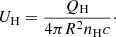 (1)
(1)Here, R is the distance between the emission source and the observed outflow component, nH is the hydrogen number density, and c is the speed of light. Using the photoionization code CLOUDY (vers. 23.01, Gunasekera et al. 2023), and following the procedure described in Edmonds et al. (2011), we compared the measured Nion values with model predictions to determine best-fit values of NH and UH.
-
Collisional excitation modeling: In seven of eight outflows, we detected troughs arising from collisionally excited levels of one or more of the following species: C II, Si II, N III, and S IV. The relative population of these excited states with respect to the ground state is an indicator of the ne of the outflow (e.g., Arav et al. 2018). Using the CHIANTI atomic database (vers. 9.0; Dere et al. 2019), we predicted the theoretical population ratios as a function of ne. By comparing these with the measured column density ratios, we derived the corresponding ne for each outflow.
Properties of the objects in our final sample.
4. Results
4.1. Physical properties of the outflowing gas
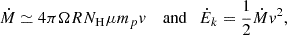
Figure 1 shows the best-fit parameters in the (NH, UH) phase space that were derived from the photoionization modeling of the outflows. The solutions span more than 2 dex in log(NH) and 1.5 dex in log(UH), and lie close to or before the hydrogen ionization front (traced roughly by the line log(NH)–log(UH) ∼ 23), consistent with the expectations for high-ionization outflows (Lucy et al. 2014). Both features are also similar to the results of the VLT sample of Xu et al. (2019) (denoted with black plus signs).
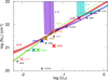 |
Fig. 1. Phase-space plot showing the NH and UH solutions for the DESI sample (colored Xs) and the VLT sample of Xu et al. (2019) (black plus signs). The colored lines and associated shaded regions indicate the Nion constraints (measurements and errors, respectively) used to derive the NH and UH solutions for the outflow detected in J1426+3151. The phase-space solution with minimized χ2 is shown as an orange cross surrounded by a black eclipse indicating the 1σ error. |
In the cases of J0542–2003 and J0857+3149, we obtained robust column density measurements for two ionic species of the same element: Al II and Al III. Their ratio allowed us to obtain the ionization state of the outflow independently of the assumed abundances. In both cases, we find that the (NH, UH) solution obtained using all measured ionic column density constraints (and assumed solar abundance) does not differ significantly from the abundance-independent solution obtained using only Al II and Al III (with Δ ∼ 0.1 dex for both parameters). This indicates that the actual gas-phase abundance in these outflows is indeed close to our initial assumption of solar values (based on Grevesse & Sauval 1998, which is the default used by CLOUDY).
Fig. 2 shows the ne obtained from the collisional excitation modeling of the outflows. Using excited states corresponding to three different ionic species over a broad range of ionization, we obtained log(ne) solutions that span over 3 dex, which is similar to the range probed by Xu et al. (2019) in their VLT sample. For some outflowing systems, we measured column densities from multiple ground- and excited-state transitions. In all of these cases, the limits and measurements obtained from the excited states were consistent; we show only the most robust determination.
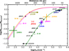 |
Fig. 2. Theoretical population ratios for different ionic species at Te = 15 000 K (solid curves). The vertical part of each cross represents the observed column density ratio and its error for each outflowing system, while the horizontal part represents the associated ne error. The arrows indicate lower limits obtained from possibly saturated troughs corresponding to these species. The case of J0542 is explained in Section 6.1. The top axis shows the distance scale based on the outflow detected in J1426+3151. The black stars and arrows correspond to objects from Xu et al. (2019). |
The ne solutions in Fig. 2 were obtained assuming a temperature of 15 000 K. In principle, since the outflows have different UH, they can have different effective temperatures. To account for this, we obtained the effective temperature in each cloud for all ionic species used in the ne determination. These temperatures span a range between 11 000 K and 17 000 K. Including this effect changes the obtained log(ne) solutions by less than 0.1 dex.
4.2. Distance and energetics
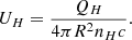
Having determined UH and ne, we used Equation (1) to calculate the distance of the outflowing components from their central source (R) as
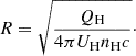 (2)
(2)
For highly ionized plasma, nH and ne are related as nH ≈ 0.8ne (Osterbrock & Ferland 2006). To calculate QH, we scaled the spectral energy distribution (SED) to match the observed flux density (Fλ) at a rest wavelength of λrest ≈ 2900 Å for each object, and then integrated the scaled SEDs for energies greater than 1 Ryd. The derived distances for the outflowing components are reported in Table 2. We find that five out of the seven outflows are located at distances greater than 200 pc, including two outflows with R > 1 kpc. For the outflows in J0857+3149 and J1229+3316, we only have upper limits on R, placing them within 100 pc and 900 pc of the central source, respectively.
The mass outflow rate (Ṁ) and the kinetic luminosity (Ėk) are given by (see Borguet et al. 2012a, for details)
 (3)
(3)
where mp is the proton mass, μ ≈ 1.4 is the mean atomic mass of the gas per proton, and Ω is the fractional solid angle covered by the outflow. Typically, the detection frequency of an outflow type across all quasar spectra is used to estimate Ω. For BAL outflows, the incidence rate is ∼20%, based on the detection of C IV (Hewett & Foltz 2003; Knigge et al. 2008). As shown by Dunn et al. (2012) using photoionization models, absorption troughs from S IV and C IV likely arise from the same physical region for a given outflow and thus have the same Ω. Therefore, we adopted Ω = 0.2 to calculate Ṁ and Ėk for the outflows in our sample and report them in Table 2. In estimating the errors, we account for the correlation between R and NH (through the error ellipse in Fig. 1), following the procedure described in Walker et al. (2022).
Outflow parameters.
4.3. The combined S IV sample
Combining the S IV objects from Xu et al. (2019) with our sample yielded a total of 15 quasars in the redshift range 2.00 ≤ z ≤ 3.15. These include 16 analyzed S IV outflows (with J1512+1119 hosting two), of which ten have robust distance (and energetics) measurements, five have upper or lower limits, and for one no constraints could be obtained. We excluded two objects from Xu et al. (2019): (i) J0825+0740, which has an outflow with positive velocity, indicating either an infall or uncertainty in the quasar redshift determination; and (ii) J1512+1119, as the R for its outflow is only constrained to within a factor of 30.
In Fig. 3, we plot the outflow distance as a function of the line-of-sight velocity, revealing that faster outflows are typically located closer to their central source. The Pearson correlation coefficient for this trend is r = −0.86, suggesting a strong negative correlation. We find that the p-value is p = 3 × 10⁻³, indicating only a ∼0.3% probability that a normal uncorrelated system could produce the observed trend. Only one data point lies in the low-velocity regime, where errors in velocity determination are significantly impacted by the accuracy of redshift determination. To ensure that this data point alone did not drive our correlation statistics, we removed it from our sample and recalculated r and p. This yielded r = −0.68 (with p = 6.3 × 10⁻²), still indicating a moderate to strong negative correlation. We performed a χ2 minimization to find the best-fit log-linear relationship (shown as the black solid line in Fig. 3), which has a slope of −0.87 and a y-intercept of 5.58. These values are similar to those obtained by Byun et al. (2024) (−1.08 and 6.44, respectively) for a sample of 24 very high-ionization absorption outflows detected in the extreme UV using HST. These observed trends are possibly a result of the outflowing gas slowing down naturally as it moves farther away and sweeps up more material, as expected in theoretical models of energy-conserving shock bubbles (see Figs. 1 and 3 of Hall et al. 2024).
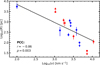 |
Fig. 3. Distribution of log(R) versus log(|v|) for the combined S IV sample. Objects analyzed in this work are shown in blue, and objects from Xu et al. (2019) are shown in red. The sample shows a strong negative correlation with a PCC of −0.86; this drops to −0.68 if the lowest velocity outflow is excluded. The black line shows the best-fit log-linear relationship, given by log(R) = −0.87 log(|v|) + 5.58. |
Next, we compared the outflow velocity and the mass outflow rate with the quasar luminosity (LBol). While more luminous quasars generally drive faster and more powerful outflows, we find the correlations of both v and Ṁ with LBol to be weak (r ∼ 0.42 and p ∼ 0.25 in both cases). This may result from the small luminosity range (≤1 dex) spanned by our sample and from the possibility that the observed luminosities could differ from their long-term averages.
5. Comparison with IFS analyses
Multiple IFS analyses have revealed large-scale spatially resolved outflows in luminous quasars. To compare the properties of these outflows with our absorption analysis, we focus on two studies that probe quasars with similar average luminosities (∼1047 erg s−1) and redshifts (∼2.5) as our combined S IV sample: Carniani et al. (2015) and Kakkad et al. (2020). The outflows in both studies are primarily traced by the λrest = 5007 Å emission feature of [O III], an ion with an ionization potential of ∼55 eV. This is similar to several key ionic species detected in our absorption sample (e.g., 47 eV for S IV and 64 eV for C IV), and thus these two manifestations are expected to trace outflowing gas with similar physical conditions (Crenshaw & Kraemer 2005; Xu et al. 2020).
In Fig. 4 we show the relation between the Ṁ of outflows and the bolometric luminosity (referred to as LAGN) of their central quasar. The samples of Carniani et al. (2015) and Kakkad et al. (2020) are shown as blue and olive circles, respectively. We find that the absorption outflows (shown as teal stars) occupy a similar region in the Ṁ − LAGN phase space as the spatially resolved ionized outflows. A similar trend emerges when comparing the outflow momentum (Ṁv) to the photon momentum of the AGN (LAGN/c) (Fig. 11 of Carniani et al. 2015), with the absorption outflows covering a wider range in outflow momentum due to their wider velocity range. The similarity between the characteristics obtained from independent analyses of the two luminosity- and redshift-matched samples provides further evidence for the connection between the emission and absorption outflows and their common physical origin (Sharma et al. 2025a; Zhao et al. 2025).
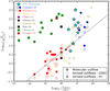 |
Fig. 4. Mass outflow rates (Ṁ) as a function of AGN bolometric luminosity (adapted from Fig. 9 of Carniani et al. 2015, with permission). Teal stars represent our combined S IV sample seen in absorption. Open and filled circles indicate the Ṁ for ionized outflows determined from [O III] and H β emission lines, respectively. Squares denote molecular outflows. |
Fig. 4 also includes ionized and molecular outflows from lower-luminosity AGN samples (from Harrison et al. 2014; Brusa et al. 2015; Cresci et al. 2015; Greene et al. 2012; Sun et al. 2014; Cicone et al. 2014; Feruglio et al. 2015). The black line shows the scaled best-fit log-linear relation obtained for ionized outflows (by Carniani et al. 2015), derived by fixing the slope to that of the molecular outflow relation from Cicone et al. (2014). As only a small sample of ionized outflows in luminous quasars had been analyzed up to this point, the intercept was mainly constrained by the low-luminosity regime. Including the sample of Kakkad et al. (2020) shows that, for ultra-luminous quasars (LAGN ≳ 1047 erg s−1), the obtained mass outflow rate is consistently underestimated by the best-fit relationship. This is supported by the results of our absorption analysis and indicates a steeper slope for ionized outflows compared to those of molecular outflows. This is consistent with the distinct scaling relations obtained by Fiore et al. (2017), who report (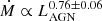 ) for molecular outflows and (
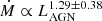 ) for ionized outflows over a broader luminosity range. The discrepancy between the mass outflow rates of molecular and ionized outflows is also highlighted by Fig. 4. At low luminosities, the ratio of molecular to ionized mass outflow rates is ∼100. Due to the steeper slope for the ionized winds, this ratio is expected to decrease with increasing luminosity. However, this trend remains poorly constrained above LAGN > 1046 erg s−1, as very few molecular outflows have been studied in such objects (e.g., Carniani et al. 2017; Spilker et al. 2025).
6. Notes on individual objects
6.1. J0542–2003: ne determination and line-locking
For the outflow analyzed in this object, we determined log(ne) =  . Unlike for other objects in our sample, this determination was not based on any single ionic species, and therefore the solution does not lie on any of the theoretical population curves in Fig. 2. This is because we obtained a lower limit based on the SiII* 1265 Å trough and an upper limit based on the non-detection of SIV* 1073 Å trough. These two limits tightly constrain the solution from both ends within 0.13 dex.
In addition to the main outflowing component analyzed in this work (S1 at –2500 km s−1), we detected three other systems through their Si IV troughs at –4400 (S2), –6300 (S3), and –8200 km s−1 (S4), as shown in Fig. 5. The separation between these distinct kinematic components (∼1900 km s−1) is similar to the velocity separation between the Si IV doublets (≈1934 km s−1). This phenomenon is referred to as line-locking and serves as an indicator of the significance of radiation pressure in driving quasar outflows (Goldreich & Sargent 1976; Braun & Milgrom 1989; Lewis & Chelouche 2023). The three new components are also detected in other high-ionization species such as C IV, N V, and O VI, while only S2 shows troughs from low-ionization species such as C II and Al III. The presence of excited states corresponding to the additional line-locked systems cannot be confidently confirmed or ruled out due to the limited resolution and S/N at shorter wavelengths. We are thus unable to constrain their distance and energetics at this stage.
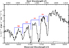 |
Fig. 5. Un-normalized DESI spectrum of J0542–2003 highlighting the multiple line-locked Si IV doublets. The four absorption systems (S1 through S4) are separated in velocity space by the same amount as the separation between the Si IV doublets, leading to the nested absorption features. |
6.2. J0845+2127: Trough variability and BAL emergence
The spectrum of J0845+2127 also contains additional kinematic components beyond the main outflowing system with v = −3800 km s−1 (S1). These include components at −6200 (S2) and –22 000 km s−1 (S3), with corresponding widths of ∼1200 km s−1 and 3000 km s−1, respectively. Both components also show troughs from other high-ionization species such as Si IV, N V, and O VI, but none from commonly detected low-ionization species. This object was also observed with SDSS on two occasions: in November 2012 and January 2018. We compared these two SDSS epochs with the DESI spectrum from January 2021, revealing interesting changes over ∼2.3 yr in the quasar rest frame. We find that the continuum flux decreased by ∼30% between the 2012 and 2018 epochs within the observed wavelength range 3600–6000 Å. Between 2018 and 2021, the continuum flux in the same wavelength range increased again by ∼25%.
To investigate any possible changes in the absorption features, we scaled the 2018 and 2021 epochs to match the continuum flux level of the 2012 epoch. For the main outflowing system (S1), we find no significant variation in the observed troughs. However, as many of the troughs corresponding to S1 are either saturated (e.g., C IV, Si IV, and N V) or lie in the spectral region where the SDSS data has low S/N (e.g., S IV, P V), we cannot rule out possible changes. Similarly, we find no appreciable variation in the troughs associated with S2. For S3, however, we find that the depth of C IV BAL increases gradually from 2012 to 2021 (as shown in top panel of Fig. 6). The Si IV 1394 Å trough detected for this system in the 2021 DESI spectrum is not detected in the SDSS spectrum from 2012. In the 2018 spectrum, a weak trough appears, which becomes deeper and wider over ∼0.9 yr in the quasar rest frame, leading to the observed trough in the 2021 spectra. A similar behavior is seen for the Si IV 1403 Å trough; however, due to contamination by a C II trough from another system, the change is less evident.
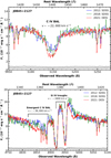 |
Fig. 6. DESI and SDSS spectra of J0845+2127 for three epochs. The continuum fluxes for the 2018 and 2021 epochs are matched to that of the 2012 SDSS spectra to highlight variability in the absorption features. The top panel shows the strengthening of C IV BAL with v ∼ −22 000 km s−1 over time. The bottom panel shows the emergence of a C IV BAL with v ∼ −39 000 km s−1 between 4820 and 4890 Å. The apparent increase in the depth of the narrow intervening features in both panels is a result of the higher resolution of the DESI spectrum. |
We also find evidence for emergence of an extremely high-velocity BAL system at v ≈ −39 000 km s−1. In the observed wavelength range 4820 Å ≲ λobs ≲ 4890 Å, increased absorption is seen in the 2021 spectrum relative to both the 2012 and 2018 spectra (as shown in bottom panel of Fig. 6). In particular, a new broad absorption feature emerges (seen most clearly for λobs ≲ 4860 Å, where no prior absorption was present) leading to a downwards shift in the narrow absorption features between 4860 and 4890 Å. This broad emergent feature does not align with any expected troughs from all other absorption systems in the spectrum (S1-3) and is therefore marked as C IV, corresponding to an extremely high-velocity outflow (based on the criterion used by Hidalgo et al. 2020). We also find N V absorption associated with this system, which shows remarkable kinematic correspondence with the absorption profile of C IV, further confirming our detection of the extremely high-velocity outflow.
The variation seen in the absorption features across the three epochs could be due to: (i) transverse motion of the outflowing gas across our line of sight (e.g., Moe et al. 2009; Hall et al. 2011) and/or (ii) a change in the ionization state of the gas (e.g., Sharma et al. 2025b). The detected pattern of variation in multiple kinematic components favors the second scenario, as suggested by Hamann et al. (2011) and Capellupo et al. (2013). This is also supported by the observed change in the continuum flux density between the epochs, which could be correlated with a change in the incident ionizing flux and, consequently, in the ionization state of the gas.
6.3. J1035+3253: Emergence of a BAL component
In the DESI spectrum of J1035+3253, the main outflowing system at v = −2570 km s−1 (S1) is accompanied by a broad (Δv ≈ 6000 km s−1) high-velocity component at v ∼ −8000 km s−1 (S2). This component is only seen in high-ionization species such as C IV, O VI, and possibly N V (which is blueshifted to the top of the Ly α emission feature and is thus hard to characterize). The object was also observed by SDSS in March 2013. We compared that spectrum with the DESI spectrum obtained in January 2021 to study any possible variations. We find that the continuum flux decreased by ∼20% between the two epochs. After scaling the DESI spectrum to match the continuum flux level of the SDSS spectrum, we find no variation for the detected troughs corresponding to S1. However, for the high-velocity component (S2), we find that the C IV trough is not detected in the SDSS spectra, and thus the BAL feature emerges between the two epochs, separated by ∼2 yr in the quasar rest frame (as shown in Fig. 7). We were unable to study any potential variation in the O VI trough associated with S2 due to low S/N of the SDSS spectrum in the wavelength range of interest. The emergence of C IV BAL could be due to a change in the ionization structure of the high-velocity outflowing gas, possibly linked to the observed change in continuum flux. However, due to the limited information on the nature of the variability, we cannot rule out transverse motion being responsible for the emergence.
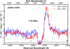 |
Fig. 7. DESI and SDSS spectra of J1035+3253 showing emergence of a C IV BAL feature with v ∼ −8000 km s−1. |
7. Discussion
7.1. Possibility of multiple ionization phases
Our photoionization modeling assumes that for a given outflowing component, all the observed ionic species can be modeled with a single ionization phase. This assumption holds for most of the observed species in the sample, except for P V, N V, and O VI. The measured column densities of P V in J0845+2127 and J1426+3151 (see Fig. 1), along with the lower limits on N V and O VI in J1021+3209, are underpredicted by the ionization phase that adequately reproduces all other observed species. This provides strong evidence for the existence of another phase with higher ionization material in at least the three above-mentioned outflows. As shown by Arav et al. (2020), this commonly occurs in outflows observable below λrest < 1050 Å, allowing for the detection of multiple species with high-ionization potential (e.g., Ne VIII, Mg X, and Si XII) that can constrain the higher ionization phase. However, for quasars at cosmic noon, DESI cannot detect troughs from such species, and we therefore lack sufficient constraints on the higher-ionization phase. This does not affect our distance determination, as the multiple phases are expected to be co-spatial due to their kinematic correspondence. However, since the higher-ionization phase is expected to have a significantly higher NH, it will carry a much larger mass (see Equation (3)). Therefore, the total energetics of the outflows are expected to be higher than the determination based on the single-phase solution.
7.2. Contribution to AGN feedback
Theoretical models and simulations have revealed that outflowing winds carrying mechanical energy equivalent to ∼5% of the quasar’s luminosity can impart sufficient energy and momentum to unbind and entrain the cold, dense interstellar medium (ISM), which dominates the total gas mass (Scannapieco & Oh 2004). In the case of “multistage” feedback, however, the outflowing winds only need to drive a significant wind in the hot, diffuse ISM, which is much less massive. Upon passing through the cold ISM, this will lead to various instabilities that shred and expand it, making it much more susceptible to “secondary” feedback from the incident quasar radiation field (Hopkins & Elvis 2010). In this scenario, the required energy input from the outflowing gas is reduced by at least an order of magnitude, to ∼0.1 − 0.5% of the quasar’s luminosity.
From our sample, the analyzed outflows in at least three objects (J0542–2003, J0845+2127, and J1426+3151) satisfy this criterion (with Ėk/LBol ≳ 0.1 − 0.5%) for significant AGN feedback, within a factor of two. For the outflow in J0857+3149, if the actual distance is close to the derived upper limit, it will also lead to a sufficiently high Ėk to enable significant feedback. Moreover, as discussed in Section 6, J0542–2003 and J0845+2127 have multiple higher-velocity outflowing components, which further contribute to the total mechanical energy output of the outflowing gas in these objects. The combined sample of 15 S IV outflows at cosmic noon (with distance determination or limits) therefore includes up to seven outflows (∼46%) that are expected to have a significant impact on their surroundings.
8. Summary
In this work, we analyzed a sample of quasar outflows at cosmic noon observed by DESI. Of 130 outflowing systems exhibiting both C IV and Si IV troughs, we confirm the detection of S IV troughs in eight, based on Monte Carlo simulations. These eight systems were subjected to detailed analysis. The main results are as follows.
-
Photoionization modeling reveals that the outflows span more than two orders of magnitude in NH and 1.5 orders of magnitude in UH, probing a wide range of ionization conditions.
-
By utilizing excited states from three different species (S IV, N III, and Si II), we obtained number density solutions for seven outflows, spanning three orders of magnitude.
-
Most outflows (at least five of the eight) are located beyond 100 pc from the central source. This includes two outflows with R > 1 kpc. For two cases, we obtained only lower limits on R, placing them at distances closer than 100 and 900 pc, respectively.
-
Analysis of the combined S IV sample (15 outflows) reveals a moderate to strong negative correlation between log(R) and log(|v|). The correlation of both v and Ṁ with LBol, however, was found to be weak.
-
The energetics of the combined S IV sample are consistent with those of spatially resolved outflows in a luminosity- and redshift-matched sample of quasars. Additionally, up to seven of the 15 analyzed outflows exhibit sufficient kinetic luminosity to contribute significantly to multistage AGN feedback processes.
As different objects in the DESI EDR are observed for varying exposure times, a smaller magnitude does not always imply higher S/N. However, through visual inspection, we found this cutoff to be sufficient for our analysis.
Acknowledgments
We acknowledge support from NSF grant AST 2106249, as well as NASA STScI grants AR-15786, AR-16600, AR-16601 and AR-17556. We thank Dr. Stefano Carniani for letting us use the right-hand panel of Fig. 9 from his Carniani et al. (2015) paper, as the base for our Fig. 4. This research uses services or data provided by the SPectra Analysis and Retrievable Catalog Lab (SPARCL) and the Astro Data Lab, which are both part of the Community Science and Data Center (CSDC) program at NSF National Optical-InfraredAstronomy Research Laboratory. NOIRLab is operated by the Association of Universities for Research in Astronomy (AURA), Inc. under a cooperative agreement with the National Science Foundation.
References
- Abareshi, B., Aguilar, J., Ahlen, S., et al. 2022, AJ, 164, 207 [NASA ADS] [CrossRef] [Google Scholar]
- Adame, A., Aguilar, J., Ahlen, S., et al. 2024, AJ, 168, 58 [NASA ADS] [CrossRef] [Google Scholar]
- Arav, N., Borguet, B., Chamberlain, C., Edmonds, D., & Danforth, C. 2013, MNRAS, 436, 3286 [NASA ADS] [CrossRef] [Google Scholar]
- Arav, N., Liu, G., Xu, X., et al. 2018, ApJ, 857, 60 [NASA ADS] [CrossRef] [Google Scholar]
- Arav, N., Xu, X., Miller, T., Kriss, G. A., & Plesha, R. 2020, ApJS, 247, 37 [Google Scholar]
- Balashev, S., Ledoux, C., Noterdaeme, P., et al. 2023, MNRAS, 524, 5016 [NASA ADS] [CrossRef] [Google Scholar]
- Bautista, M. A., Dunn, J. P., Arav, N., et al. 2010, ApJ, 713, 25 [NASA ADS] [CrossRef] [Google Scholar]
- Borguet, B. C., Edmonds, D., Arav, N., Dunn, J., & Kriss, G. A. 2012a, ApJ, 751, 107 [CrossRef] [Google Scholar]
- Borguet, B. C., Arav, N., Edmonds, D., Chamberlain, C., & Benn, C. 2012b, ApJ, 762, 49 [Google Scholar]
- Borguet, B. C., Edmonds, D., Arav, N., Benn, C., & Chamberlain, C. 2012c, ApJ, 758, 69 [NASA ADS] [CrossRef] [Google Scholar]
- Boyle, B., & Terlevich, R. J. 1998, MNRAS, 293, L49 [CrossRef] [Google Scholar]
- Braun, E., & Milgrom, M. 1989, AJ, 342, 100 [Google Scholar]
- Brusa, M., Bongiorno, A., Cresci, G., et al. 2015, MNRAS, 446, 2394 [NASA ADS] [CrossRef] [Google Scholar]
- Byun, D., Arav, N., & Hall, P. B. 2022, MNRAS, 517, 1048 [NASA ADS] [CrossRef] [Google Scholar]
- Byun, D., Arav, N., Dehghanian, M., Walker, G., & Kriss, G. A. 2024, MNRAS, 529, 3550 [NASA ADS] [CrossRef] [Google Scholar]
- Capellupo, D. M., Hamann, F., Shields, J. C., Halpern, J. P., & Barlow, T. A. 2013, MNRAS, 429, 1872 [CrossRef] [Google Scholar]
- Carniani, S., Marconi, A., Maiolino, R., et al. 2015, A&A, 580, A102 [NASA ADS] [CrossRef] [EDP Sciences] [Google Scholar]
- Carniani, S., Marconi, A., Maiolino, R., et al. 2017, A&A, 605, A105 [NASA ADS] [CrossRef] [EDP Sciences] [Google Scholar]
- Chartas, G., Cappi, M., Vignali, C., et al. 2021, ApJ, 920, 24 [NASA ADS] [CrossRef] [Google Scholar]
- Choi, H., Leighly, K. M., Terndrup, D. M., et al. 2022, ApJ, 937, 74 [NASA ADS] [CrossRef] [Google Scholar]
- Cicone, C., Maiolino, R., Sturm, E., et al. 2014, A&A, 562, A21 [NASA ADS] [CrossRef] [EDP Sciences] [Google Scholar]
- Crenshaw, D., & Kraemer, S. 2005, ApJ, 625, 680 [Google Scholar]
- Cresci, G., Mainieri, V., Brusa, M., et al. 2015, ApJ, 799, 82 [Google Scholar]
- Cresci, G., Tozzi, G., Perna, M., et al. 2023, A&A, 672, A128 [NASA ADS] [CrossRef] [EDP Sciences] [Google Scholar]
- Dai, X., Shankar, F., & Sivakoff, G. R. 2012, ApJ, 757, 180 [NASA ADS] [CrossRef] [Google Scholar]
- de Kool, M., Arav, N., Becker, R. H., et al. 2001, ApJ, 548, 609 [NASA ADS] [CrossRef] [Google Scholar]
- Dehghanian, M., Arav, N., Byun, D., Walker, G., & Sharma, M. 2024, MNRAS, 527, 7825 [Google Scholar]
- Dehghanian, M., Arav, N., Sharma, M., et al. 2025a, A&A, 695, A4 [NASA ADS] [CrossRef] [EDP Sciences] [Google Scholar]
- Dehghanian, M., Arav, N., Sharma, M., et al. 2025b, MNRAS, 540, 3086 [Google Scholar]
- Dere, K. P., Del Zanna, G., Young, P. R., Landi, E., & Sutherland, R. S. 2019, ApJS, 241, 22 [Google Scholar]
- Di Matteo, T., Springel, V., & Hernquist, L. 2005, Nature, 433, 604 [NASA ADS] [CrossRef] [Google Scholar]
- Dunn, J. P., Bautista, M., Arav, N., et al. 2010, ApJ, 709, 611 [NASA ADS] [CrossRef] [Google Scholar]
- Dunn, J. P., Arav, N., Aoki, K., et al. 2012, ApJ, 750, 143 [Google Scholar]
- Edmonds, D., Borguet, B., Arav, N., et al. 2011, ApJ, 739, 7 [NASA ADS] [CrossRef] [Google Scholar]
- Feruglio, C., Fiore, F., Carniani, S., et al. 2015, A&A, 583, A99 [NASA ADS] [CrossRef] [EDP Sciences] [Google Scholar]
- Filbert, S., Martini, P., Seebaluck, K., et al. 2024, MNRAS, 532, 3669 [NASA ADS] [CrossRef] [Google Scholar]
- Finn, C. W., Morris, S. L., Crighton, N. H., et al. 2014, MNRAS, 440, 3317 [Google Scholar]
- Fiore, F., Feruglio, C., Shankar, F., et al. 2017, A&A, 601, A143 [NASA ADS] [CrossRef] [EDP Sciences] [Google Scholar]
- Goldreich, P., & Sargent, W. 1976, Comments on Astrophysics, 6, 133 [Google Scholar]
- Greene, J. E., Zakamska, N. L., & Smith, P. S. 2012, ApJ, 746, 86 [Google Scholar]
- Grevesse, N., & Sauval, A. 1998, Space Sci. Rev., 85, 161 [NASA ADS] [CrossRef] [Google Scholar]
- Gunasekera, C. M., van Hoof, P. A., Chatzikos, M., & Ferland, G. J. 2023, RNAAS, 7, 246 [Google Scholar]
- Hall, P. B., Anosov, K., White, R., et al. 2011, MNRAS, 411, 2653 [NASA ADS] [CrossRef] [Google Scholar]
- Hall, P. B., Weiss, E., Brandt, W., & Mulholland, C. 2024, MNRAS, 528, 6496 [Google Scholar]
- Hamann, F. W., Barlow, T., Chaffee, F., Foltz, C., & Weymann, R. 2001, ApJ, 550, 142 [Google Scholar]
- Hamann, F., Kanekar, N., Prochaska, J., et al. 2011, MNRAS, 410, 1957 [Google Scholar]
- Harrison, C., Alexander, D., Mullaney, J., & Swinbank, A. 2014, MNRAS, 441, 3306 [CrossRef] [Google Scholar]
- Hewett, P. C., & Foltz, C. B. 2003, AJ, 125, 1784 [NASA ADS] [CrossRef] [Google Scholar]
- Hidalgo, P. R., Khatri, A. M., Hall, P. B., et al. 2020, ApJ, 896, 151 [CrossRef] [Google Scholar]
- Hopkins, P. F., & Elvis, M. 2010, MNRAS, 401, 7 [NASA ADS] [CrossRef] [Google Scholar]
- Hopkins, P. F., Murray, N., & Thompson, T. A. 2009, MNRAS, 398, 303 [CrossRef] [Google Scholar]
- Kakkad, D., Mainieri, V., Vietri, G., et al. 2020, A&A, 642, A147 [NASA ADS] [CrossRef] [EDP Sciences] [Google Scholar]
- Knigge, C., Scaringi, S., Goad, M. R., & Cottis, C. E. 2008, MNRAS, 386, 1426 [NASA ADS] [CrossRef] [Google Scholar]
- Leighly, K. M., Terndrup, D. M., Gallagher, S. C., Richards, G. T., & Dietrich, M. 2018, ApJ, 866, 7 [NASA ADS] [CrossRef] [Google Scholar]
- Lewis, T. R., & Chelouche, D. 2023, ApJ, 945, 110 [Google Scholar]
- Lucy, A. B., Leighly, K. M., Terndrup, D. M., Dietrich, M., & Gallagher, S. C. 2014, ApJ, 783, 58 [NASA ADS] [CrossRef] [Google Scholar]
- Madau, P., & Dickinson, M. 2014, ARA&A, 52, 415 [Google Scholar]
- Mathews, W. G., & Ferland, G. J. 1987, AJ, 323, 456 [Google Scholar]
- Matzeu, G., Brusa, M., Lanzuisi, G., et al. 2023, A&A, 670, A182 [NASA ADS] [CrossRef] [EDP Sciences] [Google Scholar]
- Miller, T. R., Arav, N., Xu, X., Kriss, G. A., & Plesha, R. J. 2020, ApJS, 247, 41 [Google Scholar]
- Moe, M., Arav, N., Bautista, M. A., & Korista, K. T. 2009, ApJ, 706, 525 [NASA ADS] [CrossRef] [Google Scholar]
- Osterbrock, D. E., & Ferland, G. J. 2006, Astrophysics Of Gas Nebulae and Active Galactic Nuclei (University science books) [Google Scholar]
- Pâris, I., Petitjean, P., Aubourg, É., et al. 2018, A&A, 613, A51 [Google Scholar]
- Planck Collaboration VI. 2020, A&A, 641, A6 [NASA ADS] [CrossRef] [EDP Sciences] [Google Scholar]
- Reeves, J., O’Brien, P. T., & Ward, M. 2003, ApJ, 593, L65 [NASA ADS] [CrossRef] [Google Scholar]
- Rigby, E., Argyle, J., Best, P., Rosario, D., & Röttgering, H. 2015, A&A, 581, A96 [NASA ADS] [CrossRef] [EDP Sciences] [Google Scholar]
- Savage, B. D., & Sembach, K. R. 1991, ApJ, 379, 245 [NASA ADS] [CrossRef] [Google Scholar]
- Scannapieco, E., & Oh, S. P. 2004, ApJ, 608, 62 [NASA ADS] [CrossRef] [Google Scholar]
- Sharma, M., Arav, N., Zhao, Q., et al. 2025a, ApJ, 983, 31 [Google Scholar]
- Sharma, M., Arav, N., Korista, K. T., et al. 2025b, A&A, 693, A254 [NASA ADS] [CrossRef] [EDP Sciences] [Google Scholar]
- Spilker, J. S., Champagne, J. B., Fan, X., et al. 2025, ApJ, 982, 72 [Google Scholar]
- Sun, A.-L., Greene, J. E., Zakamska, N. L., & Nesvadba, N. P. 2014, ApJ, 790, 160 [NASA ADS] [CrossRef] [Google Scholar]
- Walker, A., Arav, N., & Byun, D. 2022, MNRAS, 516, 3778 [NASA ADS] [CrossRef] [Google Scholar]
- Wylezalek, D., Vayner, A., Rupke, D. S., et al. 2022, ApJL, 940, L7 [Google Scholar]
- Xu, X., Arav, N., Miller, T., & Benn, C. 2018, ApJ, 858, 39 [Google Scholar]
- Xu, X., Arav, N., Miller, T., & Benn, C. 2019, ApJ, 876, 105 [NASA ADS] [CrossRef] [Google Scholar]
- Xu, X., Zakamska, N. L., Arav, N., Miller, T., & Benn, C. 2020, MNRAS, 495, 305 [NASA ADS] [CrossRef] [Google Scholar]
- Zhao, Q., Sun, L., Shen, L., et al. 2025, ApJS, 277, 57 [Google Scholar]
Appendix A: Spectral analysis
A.1. Identifying S IV troughs
Direct identification of the density sensitive S IV 1063 Å and S IV* 1073 Å troughs in quasar outflows is hindered by the dense Ly α forest, particularly for high-redshift objects (z≳ 2.5) that make up our sample. However, previous studies have shown that the kinematic profile of the S IV trough shows good correspondence with that of Si IV (Borguet et al. 2012b,c,a; Dunn et al. 2012; Arav et al. 2018; Xu et al. 2018, 2019; Dehghanian et al. 2025a). Therefore, to aid our identification, we utilize the kinematic profile of the Si IV trough (similar to the methods used by Arav et al. 2018 and Xu et al. 2019). First, we create a template of the Si IV 1403 Å trough using the apparent optical depth (AOD) model, which relates the optical depth profile with the observed residual intensity as follows:
 (A.1)
(A.1)
In cases where the Si IV 1403 Å trough is contaminated, we use the Si IV 1394 Å trough. Similarly, when the Si IV troughs appear heavily saturated, we use the Al III 1863 Å trough to obtain our template. Having obtained the template, we can create a model for the S IV trough by shifting the template to the expected wavelength. The model can thus be expressed as
 (A.2)
(A.2)
where a is a scale-factor that accounts for difference between the depths of the two troughs and λS IV, exp. is the expected wavelength of the S IV trough, which can be obtained based on the Si IV trough as (Arav et al. 2018, equation (10))
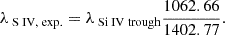 (A.3)
(A.3)
To obtain a model for the S IV trough, we set the optical depth of the deepest position of the template to 0.2 (which sets the minimum residual intensity for a trough to be detected as I≈ 0.8) and iteratively increase it in steps of 0.01 until any part of the scaled template falls below the maximum flux level allowed by the spectral data (including a 1σ noise). We compare our best-fit model with the data by using a modified χ2 (χmod2) defined as
![Mathematical equation: $$ \begin{aligned} \chi ^2_{mod} = \frac{1}{(1-\text{ min(model)})^2} \left[\frac{1}{n-1}\sum _{j}\left(\frac{\text{ model(}\textit{j}\text{)-data(}\textit{j})}{\sigma (j)}\right)^2\right] ,\end{aligned} $$](/articles/aa/full_html/2025/08/aa55291-25/aa55291-25-eq51.gif) (A.4)
(A.4)
where the sum is over all the points in the template (of which there are n) and min(model) refers to the minimum flux predicted by the template (flux corresponding to the deepest point). Within the square brackets, we have the usual definition of reduced-χ2. The modification we introduced scales the reduced χ2 such that it is lower for templates that lead to deeper troughs. They are thus preferred by our fitting-algorithm which discourages the misidentification of shallow Ly α forest features as a S IV trough.
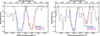 |
Fig. A.1. Example of our template fitting procedure for the absorption troughs in J1426+3151. Si IV (right panel) and S IV (left panel) troughs detected in the DESI spectrum are shown with the dashed black histograms. We performed a Gaussian fit to the Si IV 1403 trough and used its template to fit the others, while allowing for the maximum optical depth to vary. The best-fit models for all four troughs are shown with the solid lines and are accompanied by their resulting best-fit parameter. |
To further ensure that our detection of S IV is robust, we employ Monte Carlo simulations based on the Si IV template. This is done by randomly selecting 1000 wavelength points in the spectral region surrounding the expected wavelength of the S IV trough (this is typically 1038-1105 Å in the quasar rest frame). The Si IV template is shifted to each of these points individually (by replacing 1062.66 in equation A.3 with the randomly chosen test wavelength) and a corresponding best-fit model is obtained. We compare the χmod2 for these 1000 models with best-fit model at the expected S IV wavelength (equation A.3), and only claim a detection when less than 5% of the random wavelength models have a better fit to the data then the expected S IV trough (This procedure is shown visually in Fig. 5 of Arav et al. 2018). Based on this selection criteria, we find that in our sample of 130 objects that show troughs from both C IV and Si IV, a S IV trough is detected in eight of them. These eight objects (summarized in Table 1) form the final sample that is subjected to an in-depth analysis in this work.
A.2. Column density determination
For an ionic transition with rest wavelength λ (in Angstroms) and oscillator strength f, Nion can be obtained as (Savage & Sembach 1991)
![Mathematical equation: $$ \begin{aligned} N_{ion} = \frac{m_e c}{\pi e^2 f \lambda } \int \tau (v) \text{ dv} \simeq \frac{3.8 \times 10^{14}}{f \lambda } \int \tau (v) \text{ dv} \text{[cm}^{-2}] ,\end{aligned} $$](/articles/aa/full_html/2025/08/aa55291-25/aa55291-25-eq52.gif) (A.5)
(A.5)
where me is the mass of electron, c is the speed of light, e is elementary charge and τ(v) is the optical depth profile for the transition. To obtain τ(v), we used the AOD model, which assumes that the central source is completely covered by a homogeneous outflow. This relates the normalized intensity profile (I(v)) with τ(v) as  . Based on this, we modeled the detected troughs for each outflow component individually. To do so, we first modeled the Si IV 1403 Å trough with a single-Gaussian profile for τ(v) and obtain the best-fit velocity centroid (v0), width (σ), and depth (a) for the trough. We then created a template with its centroid and width fixed to the obtained best-fit parameters and used it to model all other observed troughs by varying the depth and obtain a best-fit model for each using non-linear least squares (as shown in Fig. A.1). In three of the outflows (J0542-2003, J1021+3209, J1426+3151) we find that the lower ionization species (e.g. Al II, Al III, SiII, and C II) show slight differences in kinematic features (centroid and width) as compared to the template based on the higher ionization Si IV. Similar difference in trough velocities and width based on ionization potential has been reported previously (e.g., Miller et al. 2020) and is likely a result of ions with different ionization being formed at varying depths within an outflowing cloud. In these cases, we allowed for a different template for the low-ionization species based on the Al III trough and used that to obtain the best-fit model for the remaining ions. Using equation (A.5), we then obtained the column densities for all the observed troughs based on their best-fit model.
Ionic column densities.
The AOD model used for the optical depth profile does not take into account non-black saturation effects in line centers (see section 2.2 in Arav et al. 2018, for a detailed description of non-black saturation) and can thus underestimate the column density derived from troughs that appear saturated. Therefore, in such cases, we consider the column density derived from the AOD model as a lower limit. On the other end, in some cases, we detect a shallow trough (I≲ 0.85) at the expected wavelength for a transition. As these can be significantly affected by noise, we only consider them as upper limits. Considering all these effects, we report the final column density measurements or limits for all detected trough for each outflow in Table A.1. The reported error bars include a 1σ error in the best-fit absorption models and a 20% relative error added in quadrature to account for systematic uncertainties (following Xu et al. 2018).
Appendix B: Photoionization modeling
We modeled the outflowing cloud as a plane-parallel slab of constant hydrogen number density (nH) and solar abundance, which is irradiated upon by the flux from the central source. This cloud can then be characterized by its total hydrogen column density (NH) and ionization parameter (UH), which is related to the rate of ionizing photons emitted by the source (QH) by
Here R is the distance between the emission source and the observed outflow component and c is the speed of light. QH is determined by the choice of the SED that is incident upon the outflow and the redshift of the object. For all objects in our sample (except J0845+2127; see below), we adopted the UV-soft SED of Dunn et al. (2010) and consider the effect of using different SEDs later in the section.
B.1. Determining the best-fit solution
For each object, we create a grid of models in the (NH, UH) phase space predicting the column densities of all the relevant ions at each point. These prediction are then compared to the measured ionic column densities (Nion) to constrain the phase space for each individual ionic species. The overall best-fit solution for the outflow is then determined by minimizing the χ2 between the model predictions and the actual measurements or limits.
B.2. Dependence on the SED
The choice of the incident SED is an important factor in determining the ionization and thermal structure of the outflowing gas. The UV-soft SED used primarily in our analysis was constructed by Dunn et al. (2010) based on models of accretion disk emission and improved measurements of the UV and X-ray continuum for luminous quasars (see their section 4.2 for a detailed description). To understand how sensitive our photoionization solution is to this choice, we considered the effect of two other SEDs: (i) the SED predicted by Mathews & Ferland (1987) (hereafter MF87) and (ii) the best empirically determined SED in the extreme-UV, constructed for the quasar HE 0238-1904 by Arav et al. (2013) (hereafter HE0238).
For all objects in our sample (except J0845+2127), we find that choosing either MF87 or HE0238 SED for our photoionization modeling changes the best-fit solutions for both NH and UH) (determined using the UV-soft SED) by less than 0.2 dex. In the case of J0845+2127, however, the effect is much more pronounced. This is because its photoionization solution is relatively poorly constrained as column density measurements could only be obtained from two ionic species (Al III and S IV). For the UV-Soft and MF87 SEDs, the contours corresponding to these species in the (NH, UH) phase-space plot overlap for a large range of parameters. The 1σ contours for the best-fit solution, therefore, effectively cover the entire range, making the solution unreliable. For the HE0238 SED, the overlap is over a much smaller range in parameters and thus the best-fit solution and its 1σ contour are well constrained. We thus use this solution for the rest of the analysis, while noting its strong dependence on the SED.
All Tables
All Figures
|
Fig. 1. Phase-space plot showing the NH and UH solutions for the DESI sample (colored Xs) and the VLT sample of Xu et al. (2019) (black plus signs). The colored lines and associated shaded regions indicate the Nion constraints (measurements and errors, respectively) used to derive the NH and UH solutions for the outflow detected in J1426+3151. The phase-space solution with minimized χ2 is shown as an orange cross surrounded by a black eclipse indicating the 1σ error. |
| In the text | |
|
Fig. 2. Theoretical population ratios for different ionic species at Te = 15 000 K (solid curves). The vertical part of each cross represents the observed column density ratio and its error for each outflowing system, while the horizontal part represents the associated ne error. The arrows indicate lower limits obtained from possibly saturated troughs corresponding to these species. The case of J0542 is explained in Section 6.1. The top axis shows the distance scale based on the outflow detected in J1426+3151. The black stars and arrows correspond to objects from Xu et al. (2019). |
| In the text | |
|
Fig. 3. Distribution of log(R) versus log(|v|) for the combined S IV sample. Objects analyzed in this work are shown in blue, and objects from Xu et al. (2019) are shown in red. The sample shows a strong negative correlation with a PCC of −0.86; this drops to −0.68 if the lowest velocity outflow is excluded. The black line shows the best-fit log-linear relationship, given by log(R) = −0.87 log(|v|) + 5.58. |
| In the text | |
|
Fig. 4. Mass outflow rates (Ṁ) as a function of AGN bolometric luminosity (adapted from Fig. 9 of Carniani et al. 2015, with permission). Teal stars represent our combined S IV sample seen in absorption. Open and filled circles indicate the Ṁ for ionized outflows determined from [O III] and H β emission lines, respectively. Squares denote molecular outflows. |
| In the text | |
|
Fig. 5. Un-normalized DESI spectrum of J0542–2003 highlighting the multiple line-locked Si IV doublets. The four absorption systems (S1 through S4) are separated in velocity space by the same amount as the separation between the Si IV doublets, leading to the nested absorption features. |
| In the text | |
|
Fig. 6. DESI and SDSS spectra of J0845+2127 for three epochs. The continuum fluxes for the 2018 and 2021 epochs are matched to that of the 2012 SDSS spectra to highlight variability in the absorption features. The top panel shows the strengthening of C IV BAL with v ∼ −22 000 km s−1 over time. The bottom panel shows the emergence of a C IV BAL with v ∼ −39 000 km s−1 between 4820 and 4890 Å. The apparent increase in the depth of the narrow intervening features in both panels is a result of the higher resolution of the DESI spectrum. |
| In the text | |
|
Fig. 7. DESI and SDSS spectra of J1035+3253 showing emergence of a C IV BAL feature with v ∼ −8000 km s−1. |
| In the text | |
|
Fig. A.1. Example of our template fitting procedure for the absorption troughs in J1426+3151. Si IV (right panel) and S IV (left panel) troughs detected in the DESI spectrum are shown with the dashed black histograms. We performed a Gaussian fit to the Si IV 1403 trough and used its template to fit the others, while allowing for the maximum optical depth to vary. The best-fit models for all four troughs are shown with the solid lines and are accompanied by their resulting best-fit parameter. |
| In the text | |
Current usage metrics show cumulative count of Article Views (full-text article views including HTML views, PDF and ePub downloads, according to the available data) and Abstracts Views on Vision4Press platform.
Data correspond to usage on the plateform after 2015. The current usage metrics is available 48-96 hours after online publication and is updated daily on week days.
Initial download of the metrics may take a while.