| Issue |
A&A
Volume 701, September 2025
|
|
|---|---|---|
| Article Number | A46 | |
| Number of page(s) | 10 | |
| Section | Planets, planetary systems, and small bodies | |
| DOI | https://doi.org/10.1051/0004-6361/202452601 | |
| Published online | 02 September 2025 | |
Modelling Martian moons’ surface temperature: Surface temperature variations and surface thermal emission removal from future MMX/MIRS data
1
LIRA, Observatoire de Paris/PSL, Sorbonne Université, Université Paris Cité, CY Cergy Paris Université, CNRS,
5 place Jules Janssen,
92190
Meudon,
France
2
Institute of Space and Astronautical Science, Japan Aerospace Exploration Agency, Sagamihara,
Kanagawa
2525210,
Japan
3
LATMOS, IPSL, CNRS, Université Versailles St-Quentin, Université Paris-Saclay, Sorbonne Université,
11 Bvd d’Alembert,
Guyancourt
78280,
France
★ Corresponding author: This email address is being protected from spambots. You need JavaScript enabled to view it.
Received:
14
October
2024
Accepted:
7
July
2025
Abstract
Context. The mission Martian Moons eXploration (MMX) from the Japanese space exploration agency (JAXA) will study the Martian system for three years starting from 2027. The spectro-imager MMX InfraRed Spectrometer (MIRS) will observe the surface of Phobos and Deimos in the near-infrared between 0.9 and 3.6 μm. At the surface of the Martian moons, thermal emission starts to contribute around 2.5 μm and will modify the future MIRS radiance measurements.
Aims. We propose a physical method to remove the surface thermal emission contribution from the future measured spectra from MIRS data.
Methods. The method simulates the moons’ surface temperatures locally and computes their thermal emission accounting for ephemerides and topography. We therefore developed a simulation of the absorbed flux at the moons’ surface that allows their sub-surface temperature to be computed using a 1D thermal model. We used this to estimate the emitted thermal flux in the near-infrared domain.
Results. We computed the surface temperature on the complete surface of Phobos at a lateral resolution of 3° × 3°. We found that surface temperatures on Phobos vary in the range [100, 320] K depending on the thermal and textural properties of the surface, in good agreement with previous estimations. Our results indicate that the reflected solar illumination and thermal emission from Mars increase the annual average temperature of the sub-Mars hemisphere on Phobos by 7 K. This underscores the importance of accounting for the Mars effect when modelling the thermal tail observed by MIRS. We tested the sensitivity of the method to the presence of absorption features in the spectrum and found that the method is stable as long as the absorptions are located before the thermal emission range.
Key words: radiation mechanisms: thermal / techniques: imaging spectroscopy / planets and satellites: surfaces
© The Authors 2025
 Open Access article, published by EDP Sciences, under the terms of the Creative Commons Attribution License (https://creativecommons.org/licenses/by/4.0), which permits unrestricted use, distribution, and reproduction in any medium, provided the original work is properly cited.
This article is published in open access under the Subscribe to Open model. This email address is being protected from spambots. You need JavaScript enabled to view it. to support open access publication.
1 Introduction
The Martian Moons Exploration mission MMX (JAXA) will be launched in October 2026 towards the Martian system. After its arrival in 2027, the probe will closely study the system, specifically looking at its two moons: Phobos and Deimos (Kuramoto et al. 2022). The aim of this sample return mission is to provide new insights that would help to lift the mystery around the origins of the Martian moons.
Phobos and Deimos share strong spectral similarities with D-type asteroids (Thomas 1979), and hence seem to have been captured by Mars’ gravity. However, their orbital parameters (low inclination and eccentricity) suggest a formation resulting from a large impact on Mars (Craddock 2011).
To support the MMX mission, the onboard MMX InfraRed Spectrometer (MIRS) will perform observations of the surfaces of Phobos and Deimos at a resolution of up to few meters/pixel and will record the reflected flux (Barucci et al. 2021) in the [0.9–3.6] μm range. In parallel with helping in the selection of the sampling site on Phobos, MIRS will provide spectral data to build a global map of the moons at a high spectral and spatial resolution and will allow a close analysis of the surface composition. Such precise and global analysis may hold the keys to unravelling the origins of Phobos and Deimos (Barucci et al. 2021) as it will provide new insights into their surface composition and evolution. Specifically, MIRS is designed to search for hydrated minerals and organic materials by looking at the structural hydroxyl absorption features at 2.7 μm (and their associated overtones at 1.4 and 1.8 μm) and the aliphatic–aromatic organic materials near 3.5 μm that would support the capture hypothesis. In the giant impact scenario, the precursor materials would be heated to peak temperatures exceeding 1000 K (Hyodo et al. 2017), likely resulting in the complete loss of water.
The spectral range of MIRS is also compatible with the search of anhydrous mineral signatures (0.9–1 and 2 μm) that would instead support the impact hypothesis (Craddock 2011).
Because of the low near-infrared (NIR) albedo at the Phobos and Deimos surfaces (Fornasier et al. 2024), at a heliocentric distance of 1.5 AU, the solar flux is sufficient to raise the surface temperature in the range ([130–353] K, Giuranna et al. (2011)). Therefore, its thermal emission increases above the reflected part of the spectra in a significant spectral range of MIRS data (Fraeman et al. 2014; David et al. 2024). This contribution will increase the measured flux starting from 2.5 μm (Fraeman et al. 2012, 2014) and change the shape of any measured spectra, potentially hiding absorption features, and will therefore greatly complicate the analysis and the spectral data interpretation as absorption bands associated with hydrated minerals and organics are found around ≃2.7 μm and ≃3.2 μm, respectively. During the warmest hour for a given surface, the higher measured flux after 2.5 μm will increase the spectral slope specifically in this region. Moreover, with surface temperatures varying across the Phobos surface, the spectral location and shape of this thermal tail will change within the spectrum. Therefore, a correction for the thermal emission contribution is mandatory (Clark et al. 2011) to retrieve spectral parameters specifically the spectral slope and potential absorption features, and thus interpret spectroscopic data. David et al. (2024) has already proposed a singular iterative method to retrieve the temperature from a measured spectrum based on Clark et al. (2011) and its ‘thermal tail’.
In this work, we present a different but complementary approach based on geometry, thermal modelling, and an estimation of the thermal properties of the surface to compute the surface temperature at a global scale on the moons. Although it depends strongly of the knowledge of the surface, an issue that will be fixed for the MMX mission by independent observations from the other instruments on MMX, the method would be insensitive to measurements artefacts and will be a support for more detailed analysis of the future MIRS spectra.
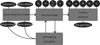 |
Fig. 1 Simple schematic of the model pipeline. The surface incoming flux is first computed in order to derive the surface temperature based on the ephemeris, the Mars albedo mosaic from Christensen et al. (2001), the shape model of the targeted moon, and its albedo. The self-heating is computed iteratively after a first run of the thermal model until the convergence is reached, reinjecting the previous estimation to compute the new surface temperature. The thermal model takes the grain size Dg, the surface porosity p and density ρ, and the non-porous thermal conductivity km and specific heat Cp as inputs. Eventually the surface thermal emission is computed for a rough surface knowing the single scattering albedo (SSA) ϖ; the surface Hapke’s average slope angle |
![Mathematical equation: $\[\bar{\theta}\]$](/articles/aa/full_html/2025/09/aa52601-24/aa52601-24-eq1.png)
2 Models
We established a simple pipeline to compute the surface emission in order to remove its contribution in the NIR spectra. We detail this pipeline below (see Fig. 1).
2.1 Estimating the absorbed flux
The first step in determining the surface temperature of the Areolian moons is to estimate the total flux reaching the surface and being absorbed by the surface. Therefore, we adapted a simulation already existing for the Cronian system (Le Gall et al. 2023; Bonnefoy et al. 2020; Leyrat et al. 2015, 2011; Ferrari & Leyrat 2006) describing how light propagates into the Martian system, accounting for the reflections between Mars and its moons. For each instant of the simulation (every 20 minutes on a seasonal cycle) the flux emitted by the Sun at the distance of Mars is computed. Thanks to the NAIF SPICE toolkit (Acton 1996; Acton et al. 2018) the geometry of the problem (i.e. the distance between objects, illumination, and reflection angles) is also computed, with respect to the position of the bodies at each time of the simulation. We mapped the moons’ surfaces with a 3 × 3°.pixel−1 (≃600 m ×600 m at the Phobos equator) grid projected onto the shape model (Willner et al. 2014) of the moons. Using the shape model allows the right incidence angle for the illumination to be computed at each coordinate of the moon and is a way to take into account the topography, and thus the associated large-scale shadowing.
The absorbed flux Fabs is computed at each time of the simulation as
![Mathematical equation: $\[\begin{aligned}F_{a b s}=(1-a_{m o o n}^{V I S}).[&F_{\odot}^{d i r}. cos (\theta_{i, \odot})+F_{\odot}^{r e f}. cos (\theta_{i, \male})] \\& +(1-a_{m o o n}^{I R}).(F_\male^{e m i}). cos (\theta_{i, \male}),\end{aligned} \]$](/articles/aa/full_html/2025/09/aa52601-24/aa52601-24-eq2.png) (1)
(1)
θi,source being the incidence angle to the local normal of the surface from the light source (Sun or Mars). It takes into account the solar flux ![Mathematical equation: $\[F_{\odot}^{d i r}\]$](/articles/aa/full_html/2025/09/aa52601-24/aa52601-24-eq3.png) at the moon heliocentric distance, the received solar flux on Mars (Mars-shine) reflected towards the moon
at the moon heliocentric distance, the received solar flux on Mars (Mars-shine) reflected towards the moon ![Mathematical equation: $\[F_{\odot}^{r e f}\]$](/articles/aa/full_html/2025/09/aa52601-24/aa52601-24-eq4.png) , and the flux emitted by Mars at its equilibrium temperature
, and the flux emitted by Mars at its equilibrium temperature ![Mathematical equation: $\[F_\male^{e m i}\]$](/articles/aa/full_html/2025/09/aa52601-24/aa52601-24-eq5.png) , and the Bond albedos in the visible and infrared
, and the Bond albedos in the visible and infrared ![Mathematical equation: $\[a_{moon}^{[Vis / I R]}\]$](/articles/aa/full_html/2025/09/aa52601-24/aa52601-24-eq6.png) (Fornasier et al. 2024).
(Fornasier et al. 2024).
Direct and reflected solar fluxes strongly depend on the heliocentric distance and the eclipses. The moon orbital period defines the simulation time step at which the absorbed flux is computed. To sample correctly the eclipses (3 per 25 h for Phobos), we set the time step to ≃22 min. The sub-Mars hemisphere ([315, 45]° E) is always irradiated by Mars thermal emission. Mars dust storms influence ![Mathematical equation: $\[F_{\odot}^{ref}\]$](/articles/aa/full_html/2025/09/aa52601-24/aa52601-24-eq7.png) and
and ![Mathematical equation: $\[F_\male^{e m i}\]$](/articles/aa/full_html/2025/09/aa52601-24/aa52601-24-eq8.png) as its surface visible albedo increases by 15% (Christensen 1988), thereby increasing the reflected light. However, the surface is no longer visible in this condition, and the Mars surface thermal emission is set to 0:
as its surface visible albedo increases by 15% (Christensen 1988), thereby increasing the reflected light. However, the surface is no longer visible in this condition, and the Mars surface thermal emission is set to 0:
![Mathematical equation: $\[F_{\odot}^{d i r}=\sigma_{S B}. T_{\odot}^4.\left(\frac{R_{\odot}}{d_{moon}}\right)^2,\]$](/articles/aa/full_html/2025/09/aa52601-24/aa52601-24-eq9.png) (2)
(2)
![Mathematical equation: $\[F_{\odot}^{r e f}=\sigma_{S B}. T_{\odot}^4.\left(\frac{R_{\odot}}{d_\male}\right)^2. a_\male^{V I S}. 2 \pi.\left(\frac{R_\male}{h_{moon}}\right)^2,\]$](/articles/aa/full_html/2025/09/aa52601-24/aa52601-24-eq10.png) (3)
(3)
![Mathematical equation: $\[F_\delta^{e m i}=\sigma_{S B}.T_{\male, e q}^4.\left(1-a_\male^{I R}\right).2 \pi.\left(\frac{R_\male}{h_{m o o n}}\right)^2.\]$](/articles/aa/full_html/2025/09/aa52601-24/aa52601-24-eq11.png) (4)
(4)
Here T⊙ and T♂,eq are respectively the temperatures of the Sun and Mars, dmoon and d♂ are the moon and Mars heliocentric distances, hmoon is the moon altitude over the Mars surface, R⊙ and R♂ are the Sun and Mars radii, and a♂ is the Mars albedo. This latest is retrieved from the Mars Global Surveyor (MGS) Thermal Emission Spectrometer (TES) global mosaic (Christensen et al. 2001).
However, we did not consider any surface albedo variation of the moons since only a low resolution albedo map exists for Deimos (Thomas et al. 1996) and is only partial for Phobos (Simonelli et al. 1998; Fornasier et al. 2024). Albedos were therefore fixed to ![Mathematical equation: $\[a_{Phobos}^{V I S}=0.0161\]$](/articles/aa/full_html/2025/09/aa52601-24/aa52601-24-eq12.png) (averaged between green and black filter from Fornasier et al. (2024)) for the visible part and
(averaged between green and black filter from Fornasier et al. (2024)) for the visible part and ![Mathematical equation: $\[a_{Phobos}^{I R}=0.02\]$](/articles/aa/full_html/2025/09/aa52601-24/aa52601-24-eq13.png) (
(![Mathematical equation: $\[a_{Phobos}^{I R}=1-e_{Phobos}^{I R}\]$](/articles/aa/full_html/2025/09/aa52601-24/aa52601-24-eq14.png) from Giuranna et al. (2011)) for the infrared part of the spectra.
from Giuranna et al. (2011)) for the infrared part of the spectra.
The flux in regions where incoming light is blocked by large-scale topographic features represented in the shape model was assumed to be zero. However, occlusion due to unresolved surface roughness was not accounted for, which may result in an overestimation of flux near the terminator. Nevertheless, this would not be a significant issue for MIRS because the measurements are likely to be limited to 60° of incidence.
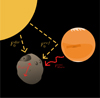 |
Fig. 2 Simple drawing gathering all flux considered in the simulation. Solar flux (direct and reflected by Mars) is indicated in yellow. Thermal emission (Mars and self-heating) is represented in red. |
2.2 Self-heating
In order to keep the model simple and to avoid too long computation times, we did not consider the self-illumination (reflections from the moon surface towards other parts of the moon) because of the low surface albedo (<5%). However, the self-heating consisting on emitted light at the surface on convex shapes cannot be neglected and is estimated.
We thus developed a simple model that computes the self-heating at the equilibrium temperature Teq (taken as the average temperature on the year after several computations of the thermal model), in which we reinject the self-heating from the previous iteration. The incident flux on a map-pixel i coming from all elements illuminating it is
![Mathematical equation: $\[F_{S H}(i)=\left(1-a_{moon}^{I R}\right). \sum_{j \neq i} \frac{\nu(i, j).\left(1-a_{moon}^{I R}\right). \sigma_{S B}. T_{e q}^4. cos(\theta_{i, j}). s_j. A_i}{d_{i, j}^2},\]$](/articles/aa/full_html/2025/09/aa52601-24/aa52601-24-eq15.png) (5)
(5)
where ν(i, j) is either 1 or 0 if the surface elements are viewing each other, θi,j represents the elements normal angular separation, sj is the surface of the ith pixel, Ai is the surface area of the ith pixel, and di,j is the estimated distance between the two elements computed on the Phobos ellipsoid.
To ensure a good convergence of the self-heating effect on the temperature, we computed the self-heating several times as a test until the average flux in the region converged. At each iteration, we reused the previous estimation of the self-heating in the computation of the new surface temperature, which was then reinjected for the new estimation of the self-heating.
At the end of the simulation, the flux absorbed by the moons was computed over an entire revolution around the Sun, which was required for thermal modelling.
2.3 Computing the surface temperature
2.3.1 A 1D thermal transfer
The surface temperature was computed over a full seasonal cycle using a thermal model developed for the thermal emission of particles inside Saturn’s ring by Ferrari & Leyrat (2006), which was then adapted to asteroids and icy satellites (Leyrat et al. 2011, 2012; Le Gall et al. 2014; Leyrat et al. 2015; Bonnefoy et al. 2020; Le Gall et al. 2023) and now for the Areolian moons.
The model solves numerically the time-dependent heat equation in 1D and considers heat transfer by conduction and radiation on the vertical axis only (from the surface towards the sub-surface) using a semi-implicit algorithm (the Crank-Nicholson method).
At the surface, the imposed limit condition is a radiative equilibrium (Eq. (6)) between the outgoing (thermal emission towards space) and incoming fluxes (solar direct, Mars-shine, Mars thermal emission, and self-heating at the surface). The temperature is considered constant at large depths Eq. (7) (deeper than ten times the seasonal thermal skin depth δth,s; adiabatic condition) and because of their size and the low energy dissipated in the moons from the Mars gravitational tides, we do not consider any endogenous heat sources (radioactive decay, tidal heating):
![Mathematical equation: $\[F_{a b s}=\left(1-a_{m o o n}^{I R}\right) \sigma_{S B}. T^4-\kappa_{e f f} \frac{\partial T}{\partial r},\]$](/articles/aa/full_html/2025/09/aa52601-24/aa52601-24-eq16.png) (6)
(6)
![Mathematical equation: $\[\left.\frac{\partial T}{\partial r}\right|_{r>10 \delta_{t h, s}}=0.\]$](/articles/aa/full_html/2025/09/aa52601-24/aa52601-24-eq17.png) (7)
(7)
Moreover, the model only considers constant thermal properties in the sub-surface, which is the main limit to this model. Because the model considers only heat transfer along the vertical axis, the maximum resolution at which the surface temperature can be estimated is approximately 10 seasonal skin depths (δth,s), which given their thermal properties, lies around 10 m on Martian moons.
The two main parameters controlling the heat transfer in the sub-surface are the effective thermal conductivity κef f and specific heat capacity Cp of the material at the surface. κef f is strongly linked to the texture of the material (namely the grain size Dg and the porosity p) as the heat transfer relies on either conduction or radiation, depending on the texture.
2.3.2 A model for the surface thermal conductivity κeff
The thermal conductivity of the surface κef f is determined following Eq. (6) from Sakatani et al. (2017), assembling the radiative and conductive terms. This relation between the texture and the thermal conductivity of the medium has been tested under vacuum conditions with glass beads as a model material for powders, for porosity ranging from 30 to 86.7% (Sakatani et al. 2017). We chose this model as it had been used in the case of microgravity for the thermal study of the Ryugu asteroid (Sakatani et al. 2018; Wada et al. 2018), and validated experimentally for high porosity (up to 86.7%) and a wide range of grain sizes up to 1000 μm and down to a few micrometres. This model assembles the two mechanisms of heat transfer: solid conductivity κsolid and radiation κrad.
The solid conductivity κsolid is determined as
![Mathematical equation: $\[\kappa_{solid}=\frac{4}{\pi^2} \kappa_m(1-p) C \xi \frac{r_c}{D_g}.\]$](/articles/aa/full_html/2025/09/aa52601-24/aa52601-24-eq18.png) (8)
(8)
Here κm represents the non-porous material thermal conductivity, p is the porosity, and C is the coordination number from Suzuki et al. (1980)
![Mathematical equation: $\[C=\frac{2.812(1-p)^{-1 / 3}}{f^2\left(1+f^2\right)},\]$](/articles/aa/full_html/2025/09/aa52601-24/aa52601-24-eq19.png) (9)
(9)
where f = 0.07318 + 2.193p − 3.357p2 + 3.194p3.
In Eq. (8), rc describes the contact radius and is defined by
![Mathematical equation: $\[r_c=\left[\frac{3\left(1+\nu^2\right)}{4 E}\left(F+\frac{3}{2} \pi \gamma D_g+\sqrt{3 \pi \gamma D_g F+\left(\frac{3}{2} \pi \gamma D_g\right)}\right)\right]^{1 / 3},\]$](/articles/aa/full_html/2025/09/aa52601-24/aa52601-24-eq20.png) (10)
(10)
where ν is Poisson’s ratio, E the Young modulus, F the external compressive force, and γ the surface energy (Johnson et al. 1971). The compressional stress expressed as ![Mathematical equation: $\[F=\frac{2 \pi D_{g}^{2}}{\sqrt{6}(1-p)} \times \rho_{0}(1-p) g z\]$](/articles/aa/full_html/2025/09/aa52601-24/aa52601-24-eq21.png) (Sakatani et al. 2017) has been neglected since its contribution in the first centimetres would be small and the thermal model does not consider variations in depth.
(Sakatani et al. 2017) has been neglected since its contribution in the first centimetres would be small and the thermal model does not consider variations in depth.
The radiative contribution to the thermal conductivity is expressed as
![Mathematical equation: $\[\kappa_{rad}=\frac{4 \epsilon}{2-\epsilon} \sigma_{S B} L T^3,\]$](/articles/aa/full_html/2025/09/aa52601-24/aa52601-24-eq22.png) (11)
(11)
where ε, σS B, and T are respectively the grain emissivity (here taken as equal to the surface emissivity), the Stefan-Boltzmann constant, and the temperature; and L is a factor describing the geometrical clearance (mean free path for radiation) in the surface, and is expressed as ![Mathematical equation: $\[L=2 \zeta\left(\frac{p}{1-p}\right)^{1 / 3} D_{g}\]$](/articles/aa/full_html/2025/09/aa52601-24/aa52601-24-eq23.png) , as described in Piqueux & Christensen (2009), ζ being a scaling factor linked to the particle size as
, as described in Piqueux & Christensen (2009), ζ being a scaling factor linked to the particle size as ![Mathematical equation: $\[\zeta=0.68+\frac{7.6 \times 10^{-5}}{D_{g}}\]$](/articles/aa/full_html/2025/09/aa52601-24/aa52601-24-eq24.png) in Sakatani et al. (2018) and Wada et al. (2018).
in Sakatani et al. (2018) and Wada et al. (2018).
2.4 Estimating the flux emitted from the rough surface
Following the method in Davidsson et al. (2015) and Davidsson & Rickman (2014), the thermal emission of a rough surface can be assimilated to the superposition of the thermal emission of a large number of facets having their own temperature due to their relative orientation to both the light source and the observer. In the case of the self-heating, this large number of facets also increase the multiple-scattering at the surface, which increases the flux budget for each facet. In addition, at large incidence angles, the facets project shadows onto their neighbours, decreasing the absorbed flux budgets and thus the temperature. Finally, the emission of the rough surface is also dependent on the geometry since facets will be hidden by their neighbours due to the roughness.
Following this approach, we simulated the emission of an unresolved roughness as the sum of the emission of Nsub sub-element within our map-pixels. Thus, we computed a large number of virtual sub-elements (Nsub = 100) within the map-pixel, each tilted at an angle θsub with respect to the map-pixel normal. This tilting angle θsub is randomly drawn from the realistic facet angle distribution computed from Hapke’s average slope parameter ![Mathematical equation: $\[\bar{\theta}\]$](/articles/aa/full_html/2025/09/aa52601-24/aa52601-24-eq25.png) , derived from the High Resolution Stereo Camera (HRSC) observation of Phobos (Fornasier et al. 2024). This angle modulates the received flux F.cos(θsub,i) in each sub-element and ensures a realistic heating due to the unresolved roughness.
, derived from the High Resolution Stereo Camera (HRSC) observation of Phobos (Fornasier et al. 2024). This angle modulates the received flux F.cos(θsub,i) in each sub-element and ensures a realistic heating due to the unresolved roughness.
To model the shadows projected by some sub-elements onto the others due to the roughness in the map-pixel, we added a term to shut down the illumination of a fraction of the sub-elements at each time step. The proportion of sub-elements in the shadows is estimated using the shadowing function S (i, e, ϕ) (Equation (12.28) from Hapke 2012). S (i, e, ϕ) depends on the geometry of illumination and observation (incidence angle i, emergence angle e, and phase angle ϕ). We computed S (i, e, ϕ) individually for each map-pixel at each time step in the simulation. The emergence angle was set to e = 0, as our goal was to estimate the number of non-illuminated sub-elements within a map-pixel only due to the unresolved roughness. However, the incidence angle i = i(t, ((λo, δo))) of a given map-pixel depends on its coordinates (λo, δo) and the local time t; the phase angle ϕ is set to ϕ = i since the shadowing function is computed in the nadir direction.
Then, for each sub-element, the temperature is computed using the thermal model described earlier.
Although it is possible to do so, we do not vary the surface texture (grain size, porosity) and composition properties from one sub-element to another; instead, we assume that the surface is homogeneous within a map-pixel.
Hence the emission of each sub-element is computed as
![Mathematical equation: $\[I_i=H(\varpi) B\left(T_i\right) B_{S H O E}\left(e_i, h_S\right),\]$](/articles/aa/full_html/2025/09/aa52601-24/aa52601-24-eq26.png) (12)
(12)
where H(ϖ) is the Chandrasekhar H function evaluated at the single scattering albedo (SSA) ϖ, B(Ti) represents the black-body emission of the sub-element i at the temperature Ti, BS HOE(ei, hS) is Hapke’s shadow hiding opposition effect (SHOE) function evaluated at the emission angle ei of the sub-element i and at the angular-width parameter hS.
Then the map-pixel emission is simply constructed as the sum of each sub-element weighted by the density of probability of the surface slope distribution a(i) giving ![Mathematical equation: $\[I_{th}={\sum}_{i}^{N} I_{i} a(i)\]$](/articles/aa/full_html/2025/09/aa52601-24/aa52601-24-eq27.png) .
.
A strong difference with the work from Davidsson et al. (2015) and Davidsson & Rickman (2014) lies in the absence, in our case, of taking the projection of shadows, which will have an important impact on temperature at large incidence angles. Additionally, we take into account the shadowing in emission in a simpler way using the Hapke’s SHOE function.
To take into account the reflective part in the spectrum, we compute the reflectance spectrum of the surface using the Hapke’s parameters derived from the observations of Phobos by HRSC.
3 Removing the surface thermal emission from spectra
3.1 Creating synthetic data
As a test of our model and in order to remove the contribution of the surface thermal emission in the spectra, we created a set of synthetic data similarly to David et al. (2024).
For each map-pixel, we simulated a sub-scale roughness similar to the one described above (see Section 2.4) to simulate the emission of a rough surface. We used the output of a thermal model to compute the surface temperature of N = 100 sub-elements, with an arbitrary value for the grain size Dg, the porosity p, the non-porous material specific heat Cp, and the thermal conductivity κm, but consistent with the Phobos. Then, we computed the map-pixel thermal emission as a superposition of the N black body (see Section 2.4).
To this black-body spectrum Ith, we added a reflective component from Hapke’s model using parameters derived from the HRSC observation (Fornasier et al. 2024). The reflectance rHapke computed from Hapke’s model was then multiplied by the solar spectrum S⊙ at Mars, and added to the thermal emission spectrum. The Hapke’s parameters that were required to compute the reflectance (namely the SHOE opposition amplitude B0, the angular half-width hs, the asymmetry parameter g, and the mean slope ![Mathematical equation: $\[\bar{\theta}\]$](/articles/aa/full_html/2025/09/aa52601-24/aa52601-24-eq28.png) ) were derived from the HRSC observation. Only the SSA ϖ was from the CRISM data (Fraeman et al. 2014). The new spectrum was then converted into I/F by dividing again by S⊙ and multiplying by π.
) were derived from the HRSC observation. Only the SSA ϖ was from the CRISM data (Fraeman et al. 2014). The new spectrum was then converted into I/F by dividing again by S⊙ and multiplying by π.
Some Gaussian noise Gnoise was then added to the spectrum to simulate the future MIRS observation S/N, the noise is taken as 1% of the I/F value at each wavelength.
The final synthetic spectrum was computed as
![Mathematical equation: $\[I / F=\pi. \frac{S_{\odot}. r_{Hapke}+I_{th}}{S_{\odot}}+G_{noise}.\]$](/articles/aa/full_html/2025/09/aa52601-24/aa52601-24-eq29.png) (13)
(13)
3.2 Test with CRISM data
To test this correction on the CRISM data, we used the cube FRT00002992_03 acquired on October 23, 2007, around 1h18 UTC. These data contain only the I/F and no correction for the observation geometry was performed.
In this observation, we defined a region of interest (RoI) close to the sub-Mars hemisphere on the Phobos surface. The choice of this RoI relies on the apparent smoothness of the area (no craters) and the constant phase angle ϕ ≃ 37°, emission angle e ≃ 5°, and incidence angle i ≃ 30°.
We used our pipeline (our flux simulation on October 23, 2007, the thermophysical model, and the thermal emission model) to compute the I/F in this RoI at the specific time of the observation. We computed the surface temperature using parameters derived from HRSC photometric observations (Fornasier et al. 2024), the non-porous material specific heat Cp = 760, and the thermal conductivity κm = 1.6 (to simulate chondritic composition (Opeil et al. 2010)), but letting the grain size Dg and the porosity p be free parameters. Once again, the Hapke model was used to compute the reflective counterpart of the spectrum.
4 Results
4.1 Flux variations at the surface of Phobos
Fig. 3 presents an output of the flux model absorbed by the Phobos surface on October 23, 2007 (at 01h17min UTC).
At the date of the simulation, the sub-solar point was lying at −20°N : 326°E, east of Stickney crater Fig. 3. The maximum flux absorbed by the Phobos surface at this date reaches 550 W m−2 on Stickney’s east rim and west inner wall.
Over the year, the instantaneous absorbed flux by the Phobos surface reaches a maximum of 718 W m−2 at the equator from external sources (the Sun and Mars). Mars-shine and Mars thermal emission contributes a maximum of 77 W m−2 on the sub-Mars hemisphere to this illumination. The self-illumination in the near-infrared by Phobos itself however adds at most an additional 34 W m−2 specifically on convex surfaces.
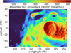 |
Fig. 3 Simulation of the fluxes absorbed by the surface of Phobos on October 23, 2007. Stickney is the large crater on the right (310°E). This simulation shows the total absorbed flux on Phobos (direct and reflected solar flux, Mars thermal emission and self-illumination). The rectangle in black is the region of interest (RoI) where we plotted the absorbed flux over the complete revolution in Fig. 4. The black pentagon represents the position of the sub-solar point at the time of the simulation. |
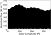 |
Fig. 4 In the RoI (black square in Fig. 3), the absorbed flux reaches 600 W.m−2, while on Phobos the maximum is 713 W m−2. A minimum of 35 W m−2 is constantly illuminating the Mars sub-point due to the Mars thermal emission. |
4.2 Surface temperature variations
A temperature global mosaic computed for Phobos October 23, 2007, at the surface with our model is presented in Fig. 5a. We set the grain size to Dg = 500 μm; the porosity to p = 50%, according to the porosity derived for Phobos in Fornasier et al. (2024); the bulk thermal conductivity to κbulk = 1.6 W m−1 K−1 to be consistent with chondritic material, in the range [1, 2] W m−1 K−1 (Opeil et al. 2010; Yomogida & Matsui 1983) measured at 200 K; and the specific heat to Cp = 760 J kg−1 K−1 (Kuzmin et al. 2003). Although Phobos surface temperatures, specifically close to the sub-solar point, are expected to be higher, eventually reaching more than 300 K, Opeil et al. (2010) stated that thermal conductivity and specific heat are somewhat constant for this temperature range. Computed at Phobos equilibrium temperature (T = 267.2 K), this gives an effective thermal conductivity of κef f = 2.710−2 W m−1 K−1, consistent with values from Kuzmin et al. (2003) where conductivity is estimated to be in the range [7.5 × 10⁻³; 2.3 × 10⁻²] W m−1 K−1. The bulk density for Phobos was set to 1873 kg cm−3 (Pieters et al. 2014; Rosenblatt 2011). Overall, the thermal inertia computed from these values and used in this work is ![Mathematical equation: $\[I_{t h}=\sqrt{\kappa_{e f f}.(1-p). \rho. C_{p}}=86 \mathrm{~J} \mathrm{~s}^{1 / 2} \mathrm{~kg}^{-1} \mathrm{~m}^{-2}\]$](/articles/aa/full_html/2025/09/aa52601-24/aa52601-24-eq30.png) , which is consistent with but slightly higher than that in previous works: 20–40 J s1/2 kg−1 m−2 from Kührt et al. (1992) and 25–85 J s1/2 kg−1 m−2 from Lunine et al. (1982).
, which is consistent with but slightly higher than that in previous works: 20–40 J s1/2 kg−1 m−2 from Kührt et al. (1992) and 25–85 J s1/2 kg−1 m−2 from Lunine et al. (1982).
As expected, an atmosphereless object where the Sun’s illumination drives the temperature, the warmest point is close to the sub-solar point −20°N : 326°E. Because of the orientation of Phobos with respect to the Sun, the boreal pole regroups the coldest area at the moon’s surface as the simulation date is set in the late northern winter (Ls = 334°).
Retrieved temperatures are consistent with previous works (Giuranna et al. 2011; Lunine et al. 1982), with a range of [130–300] K depending on the season and thus on the heliocentric distance. There is a strong dependence on the surface textural (Dg, p) and thermal properties (specific heat capacity Cp, thermal bulk conductivity κm).
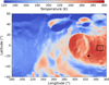 |
Fig. 5 Temperature map at Phobos on 23 October 2007 at 1h17 UTC. The sub-solar point is located on the sub-Mars hemisphere, where the warmest temperatures are recorded (288 K with the given thermal and surface properties). The rectangle in black is the region of interest presented in Fig. 3. The black pentagon represent the position of the sub-solar point at the time of the simulation. |
5 Discussion
5.1 The Mars effect
As illustrated in Fig. 4, Mars-shine and thermal emission contributes to a maximum of 77 W m−2 at sub-Mars hemisphere when Phobos is aligned between the Sun and Mars. This constant illumination of the sub-Mars hemisphere (to 35 W m−2) due to Mars thermal emission cannot be neglected in addition to the 42 W m−2 of the Mars-shine. Over the year, it raises the temperature by almost 7 K for the given surface texture and thermal properties, on the sub-Mars hemisphere.
Although 7 K may appear to be a relatively minor quantity, it nevertheless has a significant impact on the spectral amplitude and position of the thermal tail. By simulating the thermal emission spectra of black-bodies at different temperatures (285, 290, 295, and 300 K; Fig. 6b)), we found that the position of the start of the thermal tail varies by 0.1 μm every 5 K. Similarly, in the craters, the additional 35 W m−2 illuminating the craters’ inner walls increases the temperature by about 7.5 K for the given surface texture and thermal properties.
Moreover, both of these additional flux sources present the importance of other sources in the correction of the surface thermal emission in order to subtract its contribution from the future MIRS/MMX near-infrared spectra.
 |
Fig. 6 Thermal emission of a rough surface (computed from the Hapke mean slope parameter |
![Mathematical equation: $\[\bar{\theta}=24\]$](/articles/aa/full_html/2025/09/aa52601-24/aa52601-24-eq31.png)
5.2 Application to data: Comparison with black-body fitting
In this section, we develop the main goal of the paper, which is the removal of the thermal emission component in the reflectance spectra. We compare the results of our work to another method (black-body fitting) developed for the future MIRS data in David et al. (2024).
5.2.1 Removing the thermal emission in synthetic data
Following the protocol to produce synthetic data in Section 3.1, we constructed a set of data (see Fig. 7) simulating several observations to test the robustness of our thermal emission removal method. Thus, we simulated the I/F as observed on a complete day – 20 different local time around October 23, 2007, 1h17 UTC – in the RoI at eight different geometries of observation, varying the phase angle ϕ.
These synthetic data were produced for a grain size Dg = 500 μm and a porosity of p = 50%. Thermal properties κm and Cp were set respectively to 1.6 W m−1 K−1 and 760 J kg−1 K−1 to keep a chondritic material composition. These synthetic data are displayed in Fig. 7.
To test our method, we ran our thermal model at the date of the observation (October 23, 2007) for each observation time and each geometry, in order to perform a fit of the synthetic data leaving the grain size Dg and the porosity p as free parameters.
The corrected spectra presented in Figs. 7c and d show a very good removal of the thermal emission contribution for each local time and geometry of observation, the average residual slope being lower than 5 × 10⁻⁴ μm−1.
As presented in Fig. 8, we performed another test by adding absorption bands at 1.4, 2.7, and 3.4 μm, which represents potential absorption respectively from water ice, hydrated minerals (as proposed in Fraeman et al. 2014), and organic materials in order to test the sensitivity of the method to the presence of a band and to compare the variation of the band. The relative depth of the bands vary within the range [10–50]. The sensitivity of the method to the absorption band in the 2–3 μm region is critical in the MMX/MIRS context as its main objective would be to confirm or refute the presence of hydrated material, and thus to constrain the origin of Phobos. Similarly, a good correction after 3 μm will clearly help the identification of bands due to aliphatic and organic materials.
Figure 9 displays the residual slope against the relative band depth after the correction from the thermal emission. It is clear that the location of the band has a strong influence on the quality of the correction, inducing a slope up to 7 × 10⁻³ μm−1 for a deep band (50%) right in the thermal emission range (at 3.4 μm). However, the residual slope is smaller than 5% of Phobos spectral slope (2.99 × 10⁻¹ μm−1 (Fraeman et al. 2012)) in the worst case, a deep band in the thermal emission range.
One can note that the relative band depth remains unchanged in the corrected spectra, and allows a direct analysis of the surface.
Comparison with the David et al. (2024) method. We compared our correction method to the iterative black-body fitting correction described in David et al. (2024). To do so, we used the same data without any absorption band presented in Section 3.1, and ran simultaneously the iterative method and the thermophysical model. In Fig. 10, we display the residual spectra from the thermophysical method (transparent plain lines) and the iterative black-body fitting method (dash-dotted lines). We found a discrepancy between the two methods: the iterative method induces an increasing slope on the complete spectral range. This slope more likely comes from the fit performed by the iterative fitting method to remove the reflective component of the spectra. This reflective component is not simply a straight line, as it depends on the surface reflective properties at each wavelength, specifically the SSA which is increasing on Phobos (Fraeman et al. 2014).
Moreover, for the warmest hours (12AM to 14PM), the spectra present a negative slope after 3 μm which is likely due to this first fit performed to remove the reflective component of the spectrum. An error on this reflective component would indeed tilt the black body, making it more or less steep, thus degrading the fit and inducing an absorption-like feature or a negative slope in the badly fitted areas.
An easy fix to this method would be to compute the reflectance of the surface (similarly to our method) in order to get a better estimation of the reflective component of the spectrum and avoid the apparition of features of this kind.
For the sensitivity test to the presence and depth of absorption feature in the spectra, we performed the same analysis as previously (Fig. 9) and we found a much larger residual slope (5× larger), which is due to fitting a straight line as the reflective component in the spectra, as already pointed out.
The iterative method of David et al. (2024) has a positive slope in the corrected I/F spectrum below 2.6 μm because the reflected component is modelled by fitting a linear function over the limited wavelength range of 2.6–2.9 μm. This linear continuum is then subtracted from the entire synthetic data spectrum to obtain the corrected I/F spectrum shown in Fig. 10a. As a result, the positive slope observed in the corrected I/F spectrum reflects the inherent non-linearity of Phobos’s SSA spectrum (Fraeman et al. 2014), rather than an error in the thermal emission estimation. The flat slopes of the corrected I/F above 2.6 μm (Fig. 10a) show that both methods can remove the thermal emission with adequate accuracy.
Based on these results, thermophysical modelling seems to be a more appropriate solution to remove the thermal emission from the surface as it does not induce any slope, takes into account several physical surface parameters, and is less sensitive to the presence of absorption features in the spectrum, specifically when they are located outside of the thermal emission spectral range. The main issue of this thermal model lies in the knowledge about the surface properties needed to get a good estimation of the surface temperature, and its computation time (several days for a global coverage). However, the first issue will progressively be fixed with the accumulation of data from both the IDEFIX rover (Michel et al. 2022) and the other instruments on board the MMX spacecraft.
Thus, we propose that both models can be used for the future MMX/MIRS data depending on the precision expected. For on-the-fly corrections, we recommend using the iterative fitting method (David et al. 2024) as it is much faster; instead, for precise estimations of band depths, and precise fitting and removal of the thermal emission, our thermophysical approach seems more appropriate.
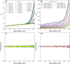 |
Fig. 7 Synthetic data created with our model following the protocol in Section 3.1 for (a) 20 different local times and (b) eight different geometries of observation varying the phase angle ϕ, with the fitted spectrum for the correction. Panels (c) and (d) show the residual spectra respectively for synthetic data after subtracting the fitted thermal emission and the assumed reflected component without the artificial absorption band. |
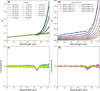 |
Fig. 8 Synthetic data created with our model following the protocol in Section 3.1 for (a) 20 different local times and (b) eight different geometries of observation, varying the phase angle ϕ, with the fitted spectrum for the correction. Panels (c) and (d) show respectively the residual spectra after removing the fitted thermal emission and the assumed reflected component with an artificial absorption band. |
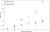 |
Fig. 9 Slope of the corrected spectra. The slope increases with the relative band depth. The location of the band also strongly changes the quality of the correction and, as expected, a band in the range 3–3.5 μm region has a strong impact on the correction. |
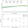 |
Fig. 10 (Panel a) Residual spectra (with offsets) after correction with our method (plain transparent), and the iterative black-body fitting from David et al. (2024) (dash-dotted lines). The synthetic data used for the comparison are the same as that presented in Fig. 7 earlier. (Panel b) Evolution of the slope residual with the presence of an absorption band in the spectra. |
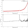 |
Fig. 11 (Panel a) CRISM spectrum of Phobos and thermophysical simulation of the surface thermal emission fitted with grain size and porosity considered as free parameters. (Panel b) Corrected spectrum with our thermal model (fitted). The method show a very noisy result after 2.9 μm. |
5.2.2 Removing the thermal emission in CRISM data
We tested both methods on real data with the spectral cube FRT00002992_03_IF162S_TRR7 observed on Phobos by CRISM (Murchie et al. 2007) on board the Mars Reconnaissance Orbiter (MRO, Zurek & Smrekar 2007) on October 23, 2007, around 1h18. Although the data are known to bear a calibration artefact around 3.18 μm (Murchie et al. 2009) in the zone 1–zone 2 filter boundary, we decided to try to remove the thermal emission in this data.
Figure 11 presents the CRISM and the simulation from our thermophysical simulation at the time of the observation (panel a). Overall, the simulation manages to reproduce quite well both the continuum [1–2.3 μm] and the thermal emission part [2.5–3.6] μm. However, we note a slight slope (2.5 × 10⁻² μm−1) induced in the range [1–2.3 μ]m by our simulation after the correction in panel b. Since this spectral range bears the reflective component only, we suppose this slope is due to uncertainties in the Hapke parameters (![Mathematical equation: $\[\bar{\theta}\]$](/articles/aa/full_html/2025/09/aa52601-24/aa52601-24-eq32.png) , SSA, B0, hs) or due to averaging the spectra in the RoI.
, SSA, B0, hs) or due to averaging the spectra in the RoI.
The correction after 2.5 μm seems reliable on the global slope displaying the same slope before 2.5 μm; however, due to the very noisy data in this region, we cannot assess the presence of absorption features. This high noise is a consequence of a calibration issue (raised in Murchie et al. 2009) due to the limit of the filters on the IR sensor blocking the grating’s high orders of diffraction. Similarly, the spike at 2.75 μm is an artefact due to the filter’s limit (Murchie et al. 2009).
6 Conclusion
We developed a model, in support of the analysis of MIRS data by the MMX mission, dedicated to estimating the surface temperature of the Martian moons in order to remove the contribution of the surface thermal emission in the future MIRS observation. This model computes the flux absorbed by the surface of the Martian moons using the available shape models, and derives the sub-surface temperature profile over a complete seasonal cycle from knowledge of the surface textural and thermal properties.
Using this model, we showed that the Mars reflected and emitted light are increasing the temperature of about 7 K and have to be considered as it would significantly change the surface thermal emission in the NIR range.
Using this thermal model, we could simulate the flux emitted by the surface of Phobos and tried to remove this emission component from the spectral data measured by CRISM. The method has been proven to be less sensitive to the presence of absorption features in the spectrum than its iterative black-body fitting counterpart, and induce fewer artefacts. However, this approach presents the inconvenience of being strongly dependent on the surface properties, and takes much more computation time than the black-body fitting method. Thus, we propose this thermophysical model as a second approach of removing the surface thermal emission in the future MIRS observation in order to perform more detailed analyses of the surface composition.
In addition to the MMX mission, this model may be seen as a proxy to probe the surface and near sub-surface texture since the grain size and the porosity will strongly influence the thermal conductivity, and thus the heat transfer inside the surface. In that case, and to improve the fit of the black body, a larger spectral range would be needed.
Acknowledgements
This work was supported by the DIM ORIGIN – Ile de France (2023) and CNES.
References
- Acton, C. H. 1996, Planet. Space Sci., 44, 65 [Google Scholar]
- Acton, C., Bachman, N., Semenov, B., & Wright, E. 2018, Planet. Space Sci., 150, 9 [Google Scholar]
- Barucci, M. A., Reess, J.-M., Bernardi, P., et al. 2021, Earth Planets Space, 73, 211 [NASA ADS] [CrossRef] [Google Scholar]
- Bonnefoy, L., Le Gall, A., Lellouch, E., et al. 2020, Icarus, 352, 113947 [Google Scholar]
- Christensen, P. R. 1988, J. Geophys. Res.: Solid Earth, 93, 7611 [Google Scholar]
- Christensen, P. R., Bandfield, J. L., Hamilton, V. E., et al. 2001, J. Geophys. Res., 106, 23823 [Google Scholar]
- Clark, R. N., Pieters, C. M., Green, R. O., Boardman, J. W., & Petro, N. E. 2011, J. Geophys. Res., 116, E00G16 [Google Scholar]
- Craddock, R. A. 2011, Icarus, 211, 1150 [NASA ADS] [CrossRef] [Google Scholar]
- David, G., Delbo, M., Barucci, M. A., et al. 2024, MNRAS, 534, 3265 [Google Scholar]
- Davidsson, B. J., & Rickman, H. 2014, Icarus, 243, 58 [NASA ADS] [CrossRef] [Google Scholar]
- Davidsson, B. J. R., Rickman, H., Bandfield, J. L., et al. 2015, Icarus, 252, 1 [Google Scholar]
- Ferrari, C., & Leyrat, C. 2006, A&A, 447, 745 [NASA ADS] [CrossRef] [EDP Sciences] [Google Scholar]
- Fornasier, S., Wargnier, A., Hasselmann, P. H., et al. 2024, A&A, 686, A203 [NASA ADS] [CrossRef] [EDP Sciences] [Google Scholar]
- Fraeman, A. A., Arvidson, R. E., Murchie, S. L., et al. 2012, J. Geophys. Res.: Planets, 117, E00J15 [Google Scholar]
- Fraeman, A., Murchie, S., Arvidson, R., et al. 2014, Icarus, 229, 196 [NASA ADS] [CrossRef] [Google Scholar]
- Giuranna, M., Roush, T., Duxbury, T., et al. 2011, Planet. Space Sci., 59, 1308 [NASA ADS] [CrossRef] [Google Scholar]
- Hapke, B. 2012, Theory of Reflectance and Emittance Spectroscopy, 2nd edn. (Cambridge, UK: New York: Cambridge University Press) [Google Scholar]
- Hyodo, R., Genda, H., Charnoz, S., & Rosenblatt, P. 2017, ApJ, 845, 125 [NASA ADS] [CrossRef] [Google Scholar]
- Johnson, K. L., Kendall, K., & Roberts, A. D. 1971, Proc. Roy. Soc. London Ser. A, 324, 301 [NASA ADS] [Google Scholar]
- Kührt, E., Giese, B., Keller, H. U., & Ksanfomality, L. V. 1992, Icarus, 96, 213 [NASA ADS] [CrossRef] [Google Scholar]
- Kuramoto, K., Kawakatsu, Y., Fujimoto, M., et al. 2022, Earth Planets Space, 74, 12 [NASA ADS] [CrossRef] [Google Scholar]
- Kuzmin, R. O., Shingareva, T. V., & Zabalueva, E. V. 2003, Sol. Syst. Res., 37, 266 [Google Scholar]
- Le Gall, A., Leyrat, C., Janssen, M., et al. 2014, Icarus, 241, 221 [Google Scholar]
- Le Gall, A. A., Bonnefoy, L. E., Sultana, R., et al. 2023, Icarus, 394, 115446 [Google Scholar]
- Leyrat, C., Coradini, A., Erard, S., et al. 2011, A&A, 531, A168 [NASA ADS] [CrossRef] [EDP Sciences] [Google Scholar]
- Leyrat, C., Barucci, A., Mueller, T., et al. 2012, A&A, 539, A154 [NASA ADS] [CrossRef] [EDP Sciences] [Google Scholar]
- Leyrat, C., Erard, S., Capaccioni, F., et al. 2015, EGU General Assembly 2015, 9767 [Google Scholar]
- Lunine, J. I., Neugebauer, G., & Jakosky, B. M. 1982, J. Geophys. Res.: Solid Earth, 87, 10297 [Google Scholar]
- Michel, P., Ulamec, S., Böttger, U., et al. 2022, Earth Planets Space, 74, 2 [NASA ADS] [CrossRef] [Google Scholar]
- Murchie, S., Arvidson, R., Bedini, P., et al. 2007, J. Geophys. Res., 112, 2006JE002682 [Google Scholar]
- Murchie, S. L., Seelos, F. P., Hash, C. D., et al. 2009, J. Geophys. Res.: Planets, 114, E00D07 [Google Scholar]
- Opeil, C., Consolmagno, G., & Britt, D. 2010, Icarus, 208, 449 [NASA ADS] [CrossRef] [Google Scholar]
- Pieters, C. M., Murchie, S., Thomas, N., & Britt, D. 2014, Planet. Space Sci., 102, 144 [CrossRef] [Google Scholar]
- Piqueux, S., & Christensen, P. R. 2009, J. Geophys. Res.: Planets, 114, E09005 [Google Scholar]
- Rosenblatt, P. 2011, Astron. Astrophys. Rev., 19, 44 [Google Scholar]
- Sakatani, N., Ogawa, K., Iijima, Y., et al. 2017, AIP Adv., 7, 015310 [Google Scholar]
- Sakatani, N., Ogawa, K., Arakawa, M., & Tanaka, S. 2018, Icarus, 309, 13 [CrossRef] [Google Scholar]
- Simonelli, D. P., Wisz, M., Switala, A., et al. 1998, Icarus, 131, 52 [NASA ADS] [CrossRef] [Google Scholar]
- Suzuki, M., Makino, K., Yamada, M., & Iinoya, K. 1980, Kagaku Kogaku Ronbunshu, 6, 59 [Google Scholar]
- Thomas, P. 1979, Icarus, 40, 223 [Google Scholar]
- Thomas, P., Adinolfi, D., Helfenstein, P., Simonelli, D., & Veverka, J. 1996, Icarus, 123, 536 [CrossRef] [Google Scholar]
- Wada, K., Grott, M., Michel, P., et al. 2018, Prog. Earth Planet. Sci., 5, 82 [Google Scholar]
- Willner, K., Shi, X., & Oberst, J. 2014, Planet. Space Sci., 102, 51 [Google Scholar]
- Yomogida, K., & Matsui, T. 1983, J. Geophys. Res.: Solid Earth, 88, 9513 [Google Scholar]
- Zurek, R. W., & Smrekar, S. E. 2007, J. Geophys. Res.: Planets, 112, E05S01 [Google Scholar]
All Figures
|
Fig. 1 Simple schematic of the model pipeline. The surface incoming flux is first computed in order to derive the surface temperature based on the ephemeris, the Mars albedo mosaic from Christensen et al. (2001), the shape model of the targeted moon, and its albedo. The self-heating is computed iteratively after a first run of the thermal model until the convergence is reached, reinjecting the previous estimation to compute the new surface temperature. The thermal model takes the grain size Dg, the surface porosity p and density ρ, and the non-porous thermal conductivity km and specific heat Cp as inputs. Eventually the surface thermal emission is computed for a rough surface knowing the single scattering albedo (SSA) ϖ; the surface Hapke’s average slope angle |
| In the text | |
|
Fig. 2 Simple drawing gathering all flux considered in the simulation. Solar flux (direct and reflected by Mars) is indicated in yellow. Thermal emission (Mars and self-heating) is represented in red. |
| In the text | |
|
Fig. 3 Simulation of the fluxes absorbed by the surface of Phobos on October 23, 2007. Stickney is the large crater on the right (310°E). This simulation shows the total absorbed flux on Phobos (direct and reflected solar flux, Mars thermal emission and self-illumination). The rectangle in black is the region of interest (RoI) where we plotted the absorbed flux over the complete revolution in Fig. 4. The black pentagon represents the position of the sub-solar point at the time of the simulation. |
| In the text | |
|
Fig. 4 In the RoI (black square in Fig. 3), the absorbed flux reaches 600 W.m−2, while on Phobos the maximum is 713 W m−2. A minimum of 35 W m−2 is constantly illuminating the Mars sub-point due to the Mars thermal emission. |
| In the text | |
|
Fig. 5 Temperature map at Phobos on 23 October 2007 at 1h17 UTC. The sub-solar point is located on the sub-Mars hemisphere, where the warmest temperatures are recorded (288 K with the given thermal and surface properties). The rectangle in black is the region of interest presented in Fig. 3. The black pentagon represent the position of the sub-solar point at the time of the simulation. |
| In the text | |
|
Fig. 6 Thermal emission of a rough surface (computed from the Hapke mean slope parameter |
| In the text | |
|
Fig. 7 Synthetic data created with our model following the protocol in Section 3.1 for (a) 20 different local times and (b) eight different geometries of observation varying the phase angle ϕ, with the fitted spectrum for the correction. Panels (c) and (d) show the residual spectra respectively for synthetic data after subtracting the fitted thermal emission and the assumed reflected component without the artificial absorption band. |
| In the text | |
|
Fig. 8 Synthetic data created with our model following the protocol in Section 3.1 for (a) 20 different local times and (b) eight different geometries of observation, varying the phase angle ϕ, with the fitted spectrum for the correction. Panels (c) and (d) show respectively the residual spectra after removing the fitted thermal emission and the assumed reflected component with an artificial absorption band. |
| In the text | |
|
Fig. 9 Slope of the corrected spectra. The slope increases with the relative band depth. The location of the band also strongly changes the quality of the correction and, as expected, a band in the range 3–3.5 μm region has a strong impact on the correction. |
| In the text | |
|
Fig. 10 (Panel a) Residual spectra (with offsets) after correction with our method (plain transparent), and the iterative black-body fitting from David et al. (2024) (dash-dotted lines). The synthetic data used for the comparison are the same as that presented in Fig. 7 earlier. (Panel b) Evolution of the slope residual with the presence of an absorption band in the spectra. |
| In the text | |
|
Fig. 11 (Panel a) CRISM spectrum of Phobos and thermophysical simulation of the surface thermal emission fitted with grain size and porosity considered as free parameters. (Panel b) Corrected spectrum with our thermal model (fitted). The method show a very noisy result after 2.9 μm. |
| In the text | |
Current usage metrics show cumulative count of Article Views (full-text article views including HTML views, PDF and ePub downloads, according to the available data) and Abstracts Views on Vision4Press platform.
Data correspond to usage on the plateform after 2015. The current usage metrics is available 48-96 hours after online publication and is updated daily on week days.
Initial download of the metrics may take a while.