© The Authors 2025

1. Introduction

The delay estimate plays a pivotal role in several fields of modern astrophysics. We roughly characterize two types of delays: “spectral” lags and “temporal” delays.

Spectral lags may be present when observing a source in different energy bands. Several factors can lead to the formation of delays between light curves obtained by two detectors under such conditions. In the case of Gamma Ray Burst (GRB), emission mechanisms can drive this effect, spanning a range from a second to even tens of seconds (Giuliani et al. 2008; Frontera et al. 2000; Tsvetkova et al. 2017). Some quantum gravity theories predict that spectral lags depend on a dispersion law for light in vacuo (Amelino-Camelia et al. 1998; Piran 2004). Delays can also be estimated between the continuum and ionized line emission (e.g., Mg II line) light curves of bright sources such as Active Galactic Nuclei (AGN). That allows for probing the AGN geometry and the spatial extent of the accretion disk using reverberation mapping techniques as in Zajaček et al. (2019). The topic of spectral lags is thoroughly discussed in the forthcoming paper Leone W. et al. (in preparation).

Gamma Ray Bursts (GRBs) are short, intense, and unrepeatable flashes of radiation, with a spectral energy distribution peaking in the gamma-ray band (D’Avanzo 2015). The theoretical isotropic energy released can reach up to 10⁵⁵ erg (Wu et al. 2012; Dado & Dar 2022), over periods ranging from fractions of a second to several thousand seconds (von Kienlin et al. 2020). However, jet-like emission in GRBs can reduce the required energy budget to produce the observed brightness by at least a factor of 100, as the energy is narrowly directed rather than spread isotopically (Sari et al. 1999). The generation of GRB is associated with the gravitational collapse of a massive star (Piran 1999; Campana et al. 2008), or the coalescence of two neutron stars in an extremely close binary system due to gravitational wave emission. In dact, the GRB 170817A event (Savchenko et al. 2017; Goldstein et al. 2017) is believed to be an example of the latter scenario. Another hypothesis proposes that the merger of a black hole and a neutron star could serve as a GRB progenitor. However, no direct observational evidence currently supports this possibility (Mochkovitch et al. 1993; Gompertz et al. 2020).

The simultaneous detection of a GRB and the emission of gravitational waves from these events marked the beginning of multi-messenger astrophysics (Mészáros et al. 2019). However, this remains the first and only GRB whose detection is associated with a gravitational wave (GW) counterpart (Abbott et al. 2017) to date.

An all-sky X-ray monitor working in tandem with a sensitive GW detector is crucial for maximizing the probability of observing multi-messenger events such as GRB 170817A (Ghirlanda et al. 2024). Precise localization of the X-ray source is essential to accurately associate the electromagnetic event with its gravitational wave counterpart. Additionally, an accurate position for such events-coincident with gravitational wave detection-enables targeted searches for counterparts in lower energy bands, such as optical or IR. In these bands, the large number of observable objects and the typically low spatial resolution make precise localization even more critical.

The High Energy Rapid Modular Ensemble of Satellites Technologic and Scientific Pathfinder (HERMES-TP/SP) is a 3U nanosatellites project based on the distributed architecture concept mission (Fiore et al. 2020). The six-unit formation is designed to monitor and localize high.energy transient sources via the triangulation method (Hurley et al. 2013; Sanna et al. 2020; Burderi et al. 2021).

Temporal delays are crucial for triangulating the position of transient events, which is the purpose of the HERMES-SP mission. Such delays arise between detectors located at different positions in space while observing the same event. The accurate and rapid localization of the events is key to a rapid and effective follow-up of the source by another in-orbit or ground-based instrument along several energy bands. This article covers the physical and mathematical tools that enable the estimation of this type of delay between two times-of-arrival (ToA) lists.

2. The cross-correlation method

Electromagnetic waves transport, at the speed of light, an amount of energy per square centimeter per second (flux ϕ) along the propagation direction. Plane waves in vacuo are associated with an energy flow whose intensity equals the modulus of the pointing vector s:

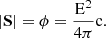$$\begin{array}{c}\hfill |\mathbf{S}|=\varphi =\frac{{\mathrm{E}}^2}{4\pi }\mathrm{c}.\end{array}$$(1)

A transitory phenomenon is, by definition, characterized by a variable flux during the occurrence of a transient source.

One can consider a scenario in which series of theoretically identical detectors can be positioned on the wavefront defined in Equation 1. Each detector measures the same intensity at the same time.

On the other hand, if the detectors are displaced arbitrarily in space each detector measures the same intensity at a delayed time, τ, which equals the scalar product of the line of propagation and the vector connecting the positions of the detectors, divided by the speed of light.

By measuring τ we can deduce the projected distances along the line of propagation and therefore, determine the direction of the wave. At least three detectors are required to determine the direction of propagation, based on geometrical considerations. This can be intuitively understood by considering that three points are sufficient to define a plane in space and, consequently, its perpendicular direction (Sanna et al. 2020). This method, known as the temporal triangulation technique (e.g. Hurley et al. 2013) relies on the experimental determination of time delays between signals observed by different detectors.

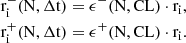
Delays can be obtained by cross-correlating two light curves-defined as the product of ϕ and the instrument’s effective area projected along the line of sight-obtained from detectors’ photons lists. To perform the cross-correlation function (CCF), a continuous function f(t) must be derived from each ToA list. Once two continuous functions, f(t), are obtained for a couple of detectors (1 and 2) the delay can be computed using the CCF:

$$\begin{array}{c}\hfill {\mathrm{CCF}}_{1,2}(\tau )={\int }_{-\infty }^{+\infty }{\mathrm{f}}_1(\mathrm{t}){\mathrm{f}}_2(\mathrm{t}+\tau )\mathrm{d}\mathrm{t}.\end{array}$$(2)

The value of τ at which $CC{F}_{1,2}(\tau )$ reaches its maximum, is the expected delay between the two light curves (MIT 2008).

It is important to note that the detector does not directly measure the intensity of the observed signal, making the derivation of the light curve from a ToA list a non-trivial task.

2.1. Statistics of times of arrival

When using a counting device (detector) the energy is recorded discretely, as a list of ToA of photons (quanta of energy). If the wave is monochromatic (single-frequency ν) each energy grain transports the same amount of energy E = hν. In the case of multi-frequency electromagnetic spectra, the same argument can be applied to the “average quanta”:

$$\begin{array}{c}\hfill ⟨\mathrm{h}\nu ⟩=\frac{{\int }_{{\nu }_{\min }}^{{\nu }_{\max }}\mathrm{h}\nu \mathrm{f}(\nu )\mathrm{d}\nu }{{\int }_{{\nu }_{\min }}^{{\nu }_{\max }}\mathrm{f}(\nu )\mathrm{d}\nu }·\end{array}$$(3)

Since we are detecting photons, we do not directly measure the variation of ϕ over time. Instead, we measure the ToA of photons associated with a given rate r(t), where r(t) represents the continuous rate at which photons are detected by the detector. The clear relation between ϕ and r is:

$$\begin{array}{c}\hfill \mathrm{r}(\mathrm{t})=\{\begin{array}{cc}\frac{\varphi (\mathrm{t})}{\mathrm{h}\nu },\hfill & \text{multi-frequency spectra}\hfill \\ \frac{\varphi (\mathrm{t})}{⟨\mathrm{h}\nu ⟩},\hfill & \text{mono-frequency spectra.}\hfill \end{array}\end{array}$$(4)

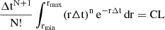
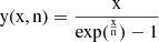
Following theorem 5.2 in Park (2018) and Appendix A we derive the normalized Poisson probability function associated with the detection of N photons within a time interval Δt, given a specific photon arrival rate r(t):

$$\begin{array}{c}\hfill {\mathrm{Q}}_{\mathrm{N},\mathrm{\Delta }\mathrm{t}}(\mathrm{r})=\mathrm{\Delta }\mathrm{t}\frac{{(\mathrm{r}\mathrm{\Delta }\mathrm{t})}^{\mathrm{N}}{\mathrm{e}}^{-\mathrm{r}\mathrm{\Delta }\mathrm{t}}}{\mathrm{N}!}·\end{array}$$(5)

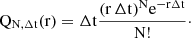
Since the detection of N photons depends on a specific rate chosen among all possible rates, we determine the corresponding confidence interval for the rate at a given confidence level (CL), in accordance with the condition described in subsection A.1. As illustrated in Figure 1, the same average rate (1 c/s) corresponds to a broader or narrower confidence interval depending on the number of observed counts. These two cases highlight how statistical regimes, defined by low or high counts, influence the accuracy of an otherwise identical rate measurement.

Fig. 1. Normalized Poisson probability function QN, Δt shown as a function of the rate r for N =1 (solid line) and n = 100 (dotted line). The gray areas indicate a confidence level (CL) of 0.68 corresponding to a 1σ CL of a Gaussian distribution.

As is standard in statistical analysis, we can define the mode (best value), average, and median of the distribution. The mode is given by$\frac{\mathrm{n}}{\mathrm{\Delta }\mathrm{t}}$ (see Appendix B) and differs from the median and the mean (defined in Appendix B). We note that, for the case n → +∞ the mode, mean, and median converge to the same value.

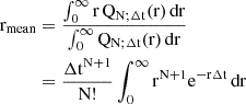
In general r_min and r_max depend on the chosen CL and can be numerically evaluated using Equation A.6 and Equation A.7, as in Appendix C.

Figure 2 shows the relative upper and lower errors associated with several CLs. The gray lines in Figure 2 correspond to the $1\pm \frac{1}{\sqrt{\mathrm{N}}}$ symmetric Gaussian relative error, at the 1 sigma CL. It is clear that, for N ≳ 10, the lower relative limit, ϵ⁻(N, 1σ CL), and the upper relative limit, ϵ⁺(N, 1σ CL), approximately equal the values of the Gaussian relative symmetric error (see, e.g., Table 1), confirming the discussion presented above.

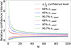Fig. 2. Relative errors (for different CLs) as a function of the observed number of events. The upper and lower limits are expressed in units of the mode rmod = N/Δt (see Appendix B for a detailed computation). The 1, 2 and 3σ confidence levels are respectively associated with 68%, 95% and 99.7%d. The gray lines represent the $\pm 1/\sqrt{\mathrm{N}}$ confidence level as a function of the observed number of events.

2.2. Construction of a light curve

If N photons are detected in a given Δt, the mode of the Poisson distribution, r = N/Δt, represents the most probable rate value whithin that interval. This value corresponds to an average rate associated with a confidence interval that depends on the chosen CL and the number of photons N, as illustrated in Figure 2.

A statistically uniform representation of a light curve can be achieved by fixing the number of photons, N, used to compute each rate point. Examining a ToA list, N photons are detected during Δt_i:

$$\begin{array}{c}\hfill {\mathrm{\Delta }\mathrm{t}}_{\mathrm{i}}={\mathrm{t}}_{\mathrm{i}·\mathrm{N}-1}-{\mathrm{t}}_{(\mathrm{i}-1)·\mathrm{N}},\end{array}$$(6)

and the corresponding rate is:

$$\begin{array}{c}\hfill r_i=\frac{\mathrm{N}}{{\mathrm{\Delta }\mathrm{t}}_{\mathrm{i}}}·\end{array}$$(7)

The time t_i associated with each rate point r_i is the barycenter of the ToA in the time interval [t_{i ⋅ N − 1},t_{(i − 1)⋅N}], i.e.,

$$\begin{array}{c}\hfill {\mathrm{t}}_{\mathrm{i}}=\frac{1}{\mathrm{N}}\sum _{\mathrm{k}=(\mathrm{i}-1)·\mathrm{N}}^{\mathrm{i}·\mathrm{N}-1}{\mathrm{t}}_{\mathrm{k}}.\end{array}$$(8)

The relative confidence interval is [ϵ⁻(N, CL), ϵ⁺(N, CL)], as shown in Figure 2 and Appendix C, and the absolute error confidence interval is

$$\begin{array}{cc}\hfill {\mathrm{r}}_{\mathrm{i}}^{-}(\mathrm{N},\mathrm{\Delta }\mathrm{t})& ={ϵ}^{-}(\mathrm{N},\mathrm{CL})·{\mathrm{r}}_{\mathrm{i}},\hfill \\ \hfill {\mathrm{r}}_{\mathrm{i}}^{+}(\mathrm{N},\mathrm{\Delta }\mathrm{t})& ={ϵ}^{+}(\mathrm{N},\mathrm{CL})·{\mathrm{r}}_{\mathrm{i}}.\hfill \end{array}$$(9)

Once N is fixed, this method guarantees the same relative accuracy for each estimated rate point.

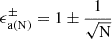
We note that the rate r_i depends on the Δt_i required to collect N photons. By increasing the number of photons N, we obtain smaller confidence intervals (see Figure 2). For N ≫ 1, the relative uncertainties converge as ${ϵ}^{-}\approx {ϵ}^{+}\approx \frac{1}{\sqrt{\mathrm{N}}}$. Increasing the accuracy of the rate measurement requires increasing N, which consequently reduces the temporal resolution.

However, the number of detected photons increases with the detector’s effective area (A_eff). Therefore, for a fixed N, an increase in A_eff allows smaller time scales to be explored with the same precision.

The method described above allows for a continuous function to be obtained by linearly connecting the rate points r_i(t_i). The light curve obtained in this way is a continuous function of the generic variable t.

2.3. Light curve variability

The variability of the light curve obtained using the method described above arises from three different phenomena:

1. The intrinsic variability of the unknown light curve, which represents the genuine variability of the source.

2. The variability induced by the Poissonian detection process. As shown in subsection 2.2 and Table 1, for N ≫ 1, the relative weight of this variability scales as the inverse of the square root of the total number N of photons used to build the light curve. In particular, in Table 1 illustrates that for N = 1 the Gaussian and the [ϵ⁻(N, CL), ϵ⁺(N, CL)] relative confidence intervals differ. For N =1, the asymptotic formula ${ϵ}_{\mathrm{a}(\mathrm{N})}^{\pm }=1\pm \frac{1}{\sqrt{\mathrm{N}}}$ overestimates the upper limit of the CL and underestimates the lower limit due to intrinsic skewness of the Poisson distribution.

3. The spurious variability introduced by the linear interpolation between rate points to generate a continuous light curve from a ToA list (see subsection 2.2). This variability is independent of the chosen N. Notably, linear interpolation between rate points introduces the minimum possible spurious variability, as it minimizes the required distance to connect consecutive rate points.

Therefore, a trade-off arises. On the one hand, we want to keep N (the number of photons used to build each light-curve point) as small as possible to exploit the detector’s minimal temporal resolution for observing the shortest intrinsic variability of the light curve. On the other hand, a larger N is required to minimize the variability induced by Poisson fluctuations. For instance, N = 10 represents a good compromise between achieving an approximately symmetric confidence interval, with reasonably small relative errors (around 30%), and exploring finer temporal resolutions.

2.4. Cross-correlation Function

Once the rate r(t) is obtained from a ToA list, the CCF can be performed between two rates, r₁(t) and r₂(t), defined for the same time interval t₁ <  t <  t₂:

$$\begin{array}{c}\hfill {\mathrm{CCF}}_{1,2}(\theta )={\int }_{{\mathrm{t}}_1}^{{\mathrm{t}}_2}{\mathrm{r}}_1(\mathrm{t}){\mathrm{r}}_2(\mathrm{t}+\theta )\mathrm{d}\mathrm{t}.\end{array}$$(10)

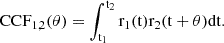
The best-fit maximum of CCF_1, 2(θ) corresponds to the best estimate of the delay $\tau$ between the two light curves:

$$max{\left\{\right|{\mathrm{CCF}}_{1,2}(\theta )\left|\right\}}_{\text{for }{t}_1<\theta <t_2}={\mathrm{CCF}}_{1,2}(\tau ).$$(11)

Since CCFs are almost symmetric functions (as shown in Figure E.1), we adopt a Gaussian profile to estimate this parameter.

3. Comparing fixed and adaptive binning for CCF

Several studies employ fixed bin-size light curves to estimate time lags using the CCF (Sanna et al. 2020) or the discrete correlation function (Castignani et al. 2014). However, adaptive binning became particularly advantageous in low-count regimes. While the techniques presented here yield results practically indistinguishable from fixed bin-size methods when applied to high-count-rate signals (e.g., > 10³ c/s), their advantages become evident when dealing with sparser data.

Figure 3 illustrates how fixed bin-size techniques exhibit clear limitations in low-count scenarios, as commonly encountered in high-energy astrophysics.

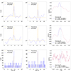Fig. 3. Top row: Light curves (left and central panels) and corresponding CCF (right panel) obtained using the adaptive rebinning method (10 photons per bin). Middle and bottom rows: Same configuration, but using fixed bin sizes of 1 s and 0.05 s, respectively. In each row, the left panel shows in blue the simulated signal obtained by rebinning the ToA list generated by simulating the theoretical profile shown in orange. The center panel displays the same signal, delayed by 1 s before rebinning. The right panel presents the CCF between the two simulated light curves shown in the left and central panels of the corresponding row.

Suppose we observe a signal with an average count rate of 10 cts/s, featuring a sharp spike lasting 0.1 s with a peak of 100 cts/s. As shown in Figure 3, fixed bin-size light curves may inadequately represent the source’s temporal variability. Using this theoretical signal, we simulated ToA lists following the procedure detailed in the next section. The resulting ToA lists were simulated under the same conditions and resemble realistic observations from an X-ray detector. If a fixed bin size of 1 s was chosen (much larger than the spike duration) the rebinning process effectively smooths out the intrinsic variability, rendering the spike invisible. Conversely, selecting a bin size of 0.05 s, comparable to the spike duration, allowed the spike to be captured. However, this came at the cost of introducing significant statistical noise: many bins contained only 0 or 1 photon, leading to substantial spurious variability unrelated to the original signal. In such cases, detecting a single photon corresponded to a 100% uncertainty in the measured rate. These issues directly impact the reliability of CCF-based delay measurements.

To further demonstrate this, we injected a 1-second delay into the theoretical signal and simulated the corresponding ToA lists. In order to estimate the expected delay, a Gaussian fit was applied to each CCF in Figure 3, centered at −1 s and spanning a width of 1 s. As clearly shown, only the adaptively binned light curves recovered the expected delay.

4. Treatment of errors

Due to the probabilistic nature of the process, when two identical detectors observe the same GRB, the obtained rates, r₁ and r₂, differ due to Poisson fluctuations. Consequently, the delay estimate τ generally differs from the expected value τ = 0 s when cross-correlating light curves of the same event as observed by two detectors positioned side by side.

For example, we considered the ToA lists associated with GRB 0908207 (see Figure 4) as observed by two Fermi-GBM detectors (NaI detector 1 and NaI detector 5: 10–900 keV). These detectors are physically separated by a maximum distance of 5 m, corresponding to the diagonal of the almost cubic shape of the Fermi satellite, which implies a maximum theoretical delay of τ_th = 15 ns (Bissaldi et al. 2009; Meegan et al. 2009). We also note that the two detectors had different pointing directions at the time of the burst. Consequently, the observed photon count and the respective respective rate varied depending on the off-axis angle relative to the source.

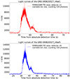Fig. 4. Light curves of GRB 090820 obtained by counting N =100 photons per bin. The upper panel shows the n1 detector light curve and the lower panel displays the n5 detector light curve.

We estimated the delay between the two detector rate curves, obtained with N = 10 and a sampling resolution of 1 μs. The CCF in Figure 5 was computed by using the procedure described above, and the CCF upper region was fitted with a Gaussian profile over a 1-second baseline. The lag estimate ${\tau }_{\exp }=(-3.5\pm 0.068)\times {10}^{-2}\mathrm{s}$ corresponds to the Gaussian best-fit parameter μ and its associated error, as shown in Figure 5. It is important to note that the delay estimation result, based on the procedures discussed in the next section, is independent of the Gaussian profile’s width.

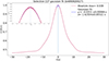Fig. 5. Upper panel: Cross-correlation function between light curves from the n1 and n5 detector ToA lists, using a variable bin size of 10 photons per bin and a 1 μs resolution. Lower panel: Zoom on the Gaussian fit centroid fluctuation relative to the vertical green dashed line, which indicates the null theoretical delays.

Taken at face value, this result would imply that some unknown systematic effect has biased the measurement. The single CCF formally yields a significant lag with minimal uncertainty, as it inherently captures the particular statistical fluctuation in the pair of detector measurements. This small uncertainty, however, is purely mathematical and pertains only to the statistical variation specific to that individual realization. Repeating the measurement under identical conditions would result in a different lag estimate due to random plot shows the CCF fluctuations.

Therefore, a Monte Carlo (MC) simulation approach is necessary to accurately estimate the overall uncertainty, incorporating the full range of possible statistical fluctuations (Zhang et al. 1999). The MC distribution of delays was centered around the best experimental estimate $\mu$ and the associated error is the standard deviation of the distribution σ.

4.1. The methods

Standard MC methods are based on simulating light curves by the ‘flux-randomization’ process, as described by Peterson et al. (1998). We explored two alternative methods for delay estimation: the Double Pool (DP) method revisits the concept of flux randomization, while the Modified Double Pool (MDP) method departs from this approach entirely, providing an experimental delay estimate without relying on simulations.

We intentionally retained the background, particularly when it is comparable to the GRB signal, since background fluctuations significantly impact the observed variability. Background subtraction would artificially enhance statistical fluctuations, potentially causing random variations to be mistaken for genuine source variability. Thus, preserving the background allowed us to evaluate variability under realistic observational conditions, avoiding the attribution of false significance to statistically insignificant features. The cross-correlation functions (CCFs) were computed over the T₉₀ and the background data intervals of 1.5 ⋅ T₉₀ before and after the T₉₀ interval. These intervals ensure that the resulting CCFs exhibit the characteristic “wings”, thus enabling a correct interpretation of any potential physical delay.

4.2. Double Pool Method: Simulation of Light curves

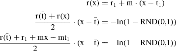
We propose an alternative method that is conceptually consistent with the real detection process of a detector. This method is based on the generalization of the inversion method in Klein & Roberts (1984) for variable light curves. Instead of using flux randomization, the proposed method generates of a simulated ToA list from a given rate curve r(t) defined over an interval t₁ <  t <  t₂:

$$\begin{array}{c}\hfill {\int }_{\mathrm{T}\_\mathrm{SIM}[\mathrm{N}-1]}^{\mathrm{T}\_\mathrm{SIM}[\mathrm{N}]}\mathrm{r}(\mathrm{t}\prime )\mathrm{dt}\prime =-\ln \{1-\mathrm{RND}(0,1)\},\end{array}$$(12)

where RND(0,1) denotes a value drawn from a uniform distribution between 0 and 1. The ToA T_SIM[N] is recursively simulated, starting from the previous time T_SIM[N − 1]. In the first step, T_SIM[N − 1] is ${\mathrm{t}}_1$. This approach emulates the detector measurement process, by applying a Poisson arrival process to the rate of the observed signal.

In the case of a constant rate r(t) = λ the integral in Equation 12 becomes:

$$\begin{array}{c}\hfill \lambda ·(\mathrm{T}\_\mathrm{SIM}[\mathrm{N}]-\mathrm{T}\_\mathrm{SIM}[\mathrm{N}-1])=-\ln \{1-\mathrm{RND}(0,1)\},\end{array}$$(13)

and each simulated time T_SIM[N] is:

$$\begin{array}{c}\hfill \mathrm{T}\_\mathrm{SIM}[\mathrm{N}]=\mathrm{T}\_\mathrm{SIM}[\mathrm{N}-1]-\frac{\ln \{1-\mathrm{RND}(0,1)\}}{\lambda }·\end{array}$$(14)

As shown in the sketch of Figure 6, the integral in Equation 12 corresponds to the area of the trapezoid between T_SIM[N − 1] and T_SIM[N], under the given rate function. According to these considerations, the Poisson arrival process T_SIM[N] can be solved analytically as in Appendix D.

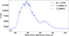Fig. 6. Luminosity curve illustrating the trapezoidal integral in Equation 12. The black point indicates a generic ToA that was just simulated in the previous step, and the red point represents the ToA to be simulated in the current step.

The net result is the generation of a ToA list, produced by a counter subject to Poissonian (quantum) fluctuations that observe the rate r(t).

4.2.1. Double Pool method

The DP method exploits this simulation technique to perform the required MC analysis between two detector ToA lists. In principle, one can use a light curve derived from a ToA list as a “theoretical” template to generate a large number of simulated light curves. However, as discussed in subsection 2.3, our “theoretical” template is affected by Poisson fluctuations that depend on the chosen value of N. This implies that, when using as a template the light curve derived by a particular ToA list as a template, Poisson fluctuations cannot be distinguished from the genuine variability of the source.

This issue can be mitigated in several ways. When estimating the CCF between two detectors, an effective approach is to use the two ToA lists to build two separate templates. Each of these templates is affected by the Poisson fluctuations discussed above. However, since these fluctuations are randomly distributed around the true rate value, any correlation between the Poisson-induced variability between the two curves is effectively removed. For a fixed, reasonable value of N (e.g., N =10) we used each of these two templates to generate several simulated ToA lists (pool of ToA lists) using the inversion method described above. We therefore performed CCF using the method described in subsection 2.4 between a pair of ToA lists, each extracted only once from each of the two pools. In this way, Poisson fluctuation variability imprinted on each template, did not correlate between the light curves and, therefore, did not bias the CCF result.

By generating a large number of ToA pairs, each belonging to one pool, and cross-correlating the corresponding light curves, we obtained a distribution of delays that was approximately Gaussian due to the central limit theorem. The mean of this distribution represents the expected delay, while the sigma indicates the uncertainty.

4.3. Modified Double Pool method

The MDP method allows one to obtain the required delay distribution while providing an exceptional computational time gain. No simulations are required to obtain this distribution. Consider a list of ToA events obtained by a detector. This list can be divided into two independent lists of ToA by generating a random number RND(0,1) for each ToA. Each ToA belongs to one of the two lists depending on the outcome of the RND(0,1). In particular, if RND(0,1) < 0.5 the ToA belongs to the first list; otherwise, it belongs to the second list. Since the spatial position of the photons on the detector area is randomly distributed with a flat distribution over the entire detection area, this splitting procedure produces two ToA lists as if obtained by two identical detectors observing the same GRB in the same spatial position, each with an effective area that is half the original one. Cross-correlating the two light curves derived from these ToA lists yields a temporal delay that fluctuates around the expected null value. These fluctuations are purely statistical in origin.

By repeating the splitting procedure with different random realizations two new ToA lists are obtained. We note that this second couple is not fully statistically independent of the first one, as the original ToA list remains unchanged. However, this statistical dependence is weak because each point in the light curve is constructed using a large number of photons (N ∼ 10), and it does not significantly affect the computation of the sigma of the distribution, as demonstrated by numerical computation (see subsection 5.2).

By averaging each rate point over N photons, each resulting light curve within the same pool represents a distinct Poissonian realization, with each rate value and associated time being approximately statistically independent of any other realization.

By recursively applying this method we obtain a pool of nearly statistically independent ToA lists from the detector. We explicitly note that the splitting is necessary only to obtain statistically independent ToA lists and the fact that this method produces a pair at each step is irrelevant to the statistical independence of the final sample of ToA lists in the pool.

Now consider a second detector observing the source. The procedure described above can be applied to obtain a pool of nearly statistically independent ToA lists.

We can now cross-correlate light curves, each extracted from one of the two pools as depicted in Figure 7. The average value of this distribution represents the expected delay and the sigma represents the associated uncertainty.

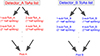Fig. 7. Scheme of the MDP splitting procedure.

5. DP and MDP testing

Gamma Ray Burts (GRBs) are optimal candidates for testing the capability of the developed tools. We aimed to obtain experimental delays that are consistent with the expected true delays. The GRB sample was randomly selected from bursts observed by Fermi-GBM, considering a broad range of fluence values. As shown in Figure E.1, the discussed CCF techniques ensure a Gaussian profile under all flux and background conditions.

To this end, the test allowed us to discriminate between the proposed procedures, defining the most effective model. During the test, the Gaussian fit guess parameters were fixed for both methods. The number of photons per bin, used to construct the light curves, was set to N =10.

5.1. MDP and DP methods comparison

To demonstrate the effectiveness of the two methods, we considered a representative sample of 20 GRBs observed by one Fermi-GBM detector. For each GRB, two independent ToA lists were generated by randomly splitting the considered Fermi-GBM detector data. This approximately corresponded to having two ToA lists with nearly half the effective area of the GBM detector (e.g., as observed by two HERMES detectors). We applied the MDP and DP methods to each pair of ToA lists. The expected theoretical temporal delay between the two ToA lists must be zero (see the discussion in Section 4).

Figure 10 compares the results of the two MC methods applied to the considered sample. Both methods accurately estimate the delays statistically compatible with the true zero delay, considering the standard deviation of each distribution. The residual histograms are compatible with zero.

As evident from Figure 10 and Figure E.1, the precision of the estimated delays decreases as the number of photons associated with the source diminishes relative to the background.

The Gaussian fit of the residual Dp distribution indicates that the DP method is less accurate in ensuring compatibility with the true delay. This discrepancy may stem from the simulation process used in the MC procedure. Specifically, the ToA lists from the two starting detectors were employed to define the initial templates for the DP method, which were then fixed during the MC simulations. Since the templates remained fixed throughout the MC simulations, any injected Poisson variability may propagate through all the simulated light curves. This may result in an MC distribution influenced by the Poissonian variability of the initially generated templates. In contrast, in the MDP method, uses reshuffling of the ToA which ensures that no privileged light curves are considered.

The MDP method effectively mitigates intrinsic Poisson fluctuations in the input templates used by standard flux randomization methods or the DP method. These fluctuations would otherwise propagate and amplify across all MC realizations, with a stronger effect as the chosen number of photons per bin decreases. While the method requires halving the available data at each step, resulting in an average loss of precision of approximately $\sqrt{2}$, it prevents the artificial amplification of Poisson noise. Consequently, it removes eventual bias in delay estimation introduced by Poissonian fluctuations in the original templates.

5.2. Demonstrating the indipendence of the that MDP

Each MDP step is statistically independent, even though the split ToA lists are always derived from the same set of events. Due to the random nature of the halving procedure, each generated light curve represents a specific Poisson realization of the true signal light curve. As a result, each delay constitutes an independent estimate, forming a delay distribution with the correct associated error, as shown in Figure 10.

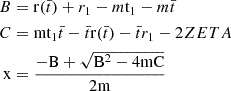
To demonstrate this, we used data from the Insight-Hard X-ray Modulation Telescope (Insight-HXMT) instrument (Zhang et al. 2018, 2020), specifically focusing on GRB 180113C in the 1–600 keV energy band. With an effective area of approximately 5000 cm², we randomly split the initial ToA list into 200 independent sub-lists. These truly correspond to the lists obtained by 200 detectors observing the same GRB under identical conditions (effective area, detector response, attitude, off-axis angle) and spatial location. We injected a 1 s delay into 100 ToA and applied CCF techniques to estimate delays between the delayed and not delayed groups. The resulting distribution of 100 values is shown in Figure 8, with an average of $\mu =-0.95\mathrm{s}$ and an associated error of σ = 0.295 s.

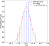Fig. 8. Delay distribution is obtained by cross-correlating 100 pairs of ToA lists, derived from the random division of the GRB 180113418 event file. A 1-second delay is injected into one of the ToA lists in each pair.

This experiment remains conceptual, as 200 identical detectors observing the same source are not available. Typically, we estimate the delay between two instruments, so for this analysis, we randomly selected two lists from the sample of 200. We again injected a 1 s delay in one of the two lists and the MDP method in Figure 7 was applied to estimate the delay.

The distribution in Figure 9 is centered at $\mu =-1.1\mathrm{s}$ with an associated error of σ = 0.299 s. This result demonstrates the efficiency of the MDP method in estimating the actual existing delays and their associated errors. Moreover, the standard deviation is approximately the same as in the previous case. This indicates that the MDP estimates are accurate even though the generated lists are not strictly statistically indipendent due to the reshuffling of the same ToA.

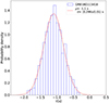Fig. 9. Delay distribution obtained by applying the MDP method to two of the 200 ToA lists derived from the random division of the GRB 180113418 event file. A 1-second delay is introduced into one ToA list. The MDP procedure is carried out by randomly splitting the initial ToA lists 500 times, resulting in two pools of 1000 light curves each.

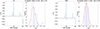Fig. 10. Comparison of DP and MDP methods. Left panels: Experimental delays estimated via MC procedures with associated errors shown as vertical error bars. Right panels: Residual distribution for each method in units of sigma.

6. Conclusion

Deriving the light curve associated with the observation of a cosmic source is a nontrivial task that requires careful handling of detector data. This step is critical in timing astronomy where delays between ToA lists from different detectors are estimated via cross-correlation since this tool is defined on continuous functions. The proposed variable bin size method facilitates the construction of “averaged” light curves from ToA data, sampling the observed electromagnetic signal with uniform statistical accuracy. This approach allows sampling the light curve at a finer temporal resolution when the intensity is higher. By applying linear interpolation between the rate points of the sampled curves, it is possible to obtain a rate function, enabling the estimation of delays via cross-correlation on continuous functions. It is important to note that linear interpolation introduces minimal variability between consecutive rate points.

The MDP Monte Carlo procedure enables the generation of a distribution of delays, where the mean is the experimental value of the delay and the standard deviation is the associated experimental error.

Our result confirm the ability of the MDP method to deliver reliable scientific results, providing a significant increase in both accuracy and computational efficiency. We conclude that the MDP method reduces the impact of intrinsic Poisson fluctuations in input templates, preventing their amplification in Monte Carlo simulations. Despite a $\sqrt{2}$ loss in precision due to halved statistics, it ensures unbiased delay estimates.

Furthermore, the developed techniques demonstrate crucial effectiveness in low-statistics regimes, where traditional methods may struggle to yield consistent results. These techniques remain effective regardless of the transient signal luminosity, although the precision of the estimated lag improves with the increasing number of source-associated photons.

The entire package, written in Python, is publicly available on the GitHub platform.

Acknowledgments

This article was produced while attending the PhD program in PhD fin Space Science and Technology at the University of Trento, Cycle XXXVIII. A.T. acknowledges financial support from “ASI-INAF Accordo Attuativo HERMES Pathinder operazioni n. 2022-25-HH.0” and the basic funding program of the Ioffe Institute FFUG-2024-0002. We sincerely thanks Cristiano Guidorzi for his valuable comments and discussions.

References

Appendix A: normalized Poisson Probability Function

The detection process is a probabilistic process in which the infinitesimal probability of detecting a photon within an infinitesimal time interval dt is:

$$\begin{array}{c}\hfill \mathrm{dP}(\mathrm{t})=\mathrm{r}(\mathrm{t})\mathrm{dt}.\end{array}$$(A.1)

The probability to detect N photons in a time Δt for a given rate $\mathrm{r}(\mathrm{t})$ is (Kingman & Taylor 1966; Pishro-Nik 2014; Dekking et al. 2005):

$$\begin{array}{c}\hfill \mathrm{P}(\mu ,\mathrm{N})=\frac{{\mu }^{\mathrm{N}}{\mathrm{e}}^{-\mu }}{\mathrm{N}!}={\mathrm{P}}_{\mathrm{N},\mathrm{\Delta }\mathrm{t}}(\mathrm{r}),\end{array}$$(A.2)

where $\mu (\mathrm{t})=\mathrm{r}(\mathrm{t})\mathrm{\Delta }\mathrm{t}$ and we assumed that $\mathrm{\Delta }\mathrm{t}$ is small with respect to the time scale on which $\mu (\mathrm{t})$ varies. Therefore:

$$\begin{array}{c}\hfill {\mathrm{P}}_{\mathrm{N},\mathrm{\Delta }\mathrm{t}}(\mathrm{r})=\frac{{(\mathrm{r}\mathrm{\Delta }\mathrm{t})}^{\mathrm{N}}{\mathrm{e}}^{-\mathrm{r}\mathrm{\Delta }\mathrm{t}}}{\mathrm{N}!}.\end{array}$$(A.3)

Equation A. 3 represents the probability of detecting N photons in a time interval Δt given a rate r(t). Apart from the overall normalization factor, Equation A. 3 can be interpreted as the probability that N photons, detected in a time interval $\mathrm{\Delta }\mathrm{t}$, derive from a particular rate $\mathrm{r}(\mathrm{t})$. Since the detection of N photons must depend on a rate, among all the possible rates, the normalization factor A is obtained by integrating Equation A. 3 in rate between 0 and ∞:

$$\begin{array}{c}\hfill \mathrm{A}{\int }_0^{+\infty }{\mathrm{P}}_{\mathrm{N},\mathrm{\Delta }\mathrm{t}}(\mathrm{r})\mathrm{dr}=1,\end{array}$$(A.4)

which gives $A=\frac{1}{\mathrm{\Delta }\mathrm{t}}$.

Therefore, given that N photons are detected within a time interval $\mathrm{\Delta }\mathrm{t}$, the probability distribution of the rate r is:

$$\begin{array}{c}\hfill {\mathrm{Q}}_{\mathrm{N},\mathrm{\Delta }\mathrm{t}}(\mathrm{r})=\mathrm{\Delta }\mathrm{t}\frac{{(\mathrm{r}\mathrm{\Delta }\mathrm{t})}^{\mathrm{N}}{\mathrm{e}}^{-\mathrm{r}\mathrm{\Delta }\mathrm{t}}}{\mathrm{N}!}.\end{array}$$(A.5)

A.1. Statistical Confidence Level

To evaluate the confidence level (CL) for the rate (as in any statistical treatment), we must integrate Equation 5 between two points of equal probability, one below and one above the (unique) maximum of the distribution. Notably, in the case of N = 0, the function simplifies to e^−rΔt, which is monotonically decreasing, allowing us to determine an upper limit.

By this definition, the CL corresponds to the area under the normalized probability distribution $Q_{N,\mathrm{\Delta }\mathrm{t}}(r)$, enclosed between the upper and lower bounds of the rate confidence interval:

$$\begin{array}{c}\hfill \mathrm{CL}={\int }_{{\mathrm{r}}_{\min }}^{{\mathrm{r}}_{\max }}{\mathrm{Q}}_{\mathrm{N},\mathrm{\Delta }\mathrm{t}}(\mathrm{r})\mathrm{dr},\end{array}$$(A.6)

with the constraint:

$$\begin{array}{c}\hfill {\mathrm{Q}}_{\mathrm{N},\mathrm{\Delta }\mathrm{t}}({\mathrm{r}}_{\min })={\mathrm{Q}}_{\mathrm{N},\mathrm{\Delta }\mathrm{t}}({\mathrm{r}}_{\max }).\end{array}$$(A.7)

Appendix B: Poisson characteristic values

B.1. Mode

The Poisson mode is the rate value where the $\mathrm{Q}(\mathrm{r}\mathrm{\Delta }\mathrm{t};\mathrm{N})$ is maximum, $\frac{\partial Q_{\mathrm{N};\mathrm{\Delta }\mathrm{t}}(\mathrm{r})}{\partial \mathrm{r}}{|}_{\mathrm{r}={\mathrm{r}}_{\mathrm{mode}}}=0$ :

$$\begin{array}{c}\hfill \frac{\mathrm{\Delta }{\mathrm{t}}^2}{\mathrm{N}!}{\mathrm{e}}^{-{\mathrm{r}}_{\mathrm{mod}}\mathrm{\Delta }\mathrm{t}}[\mathrm{N}{({\mathrm{r}}_{\mathrm{mod}}\mathrm{\Delta }\mathrm{t})}^{\mathrm{N}-1}-{({\mathrm{r}}_{\mathrm{mod}}\mathrm{\Delta }\mathrm{t})}^{\mathrm{N}}]=0\end{array}$$(B.1)

that leads to $\mathrm{N}{({\mathrm{r}}_{\mathrm{mod}}\mathrm{\Delta }\mathrm{t})}^{\mathrm{N}-1}={({\mathrm{r}}_{\mathrm{mod}}\mathrm{\Delta }\mathrm{t})}^{\mathrm{N}}$, so the mode value is

$${\mathrm{r}}_{\mathrm{mod}}(\mathrm{N},\mathrm{\Delta }\mathrm{t})=\frac{\mathrm{N}}{\mathrm{\Delta }\mathrm{t}}$$

B.2. Median

The Poisson median divides the area under the Poisson distribution into two identical parts (x = rΔt):

$$\begin{array}{c}\hfill {\int }_0^{{\mathrm{r}}_{\mathrm{med}}}\mathrm{Q}(\mathrm{r}\mathrm{\Delta }\mathrm{t};\mathrm{N})\mathrm{dr}=\frac{\mathrm{\Delta }\mathrm{t}}{\mathrm{N}!}{\int }_0^{{\mathrm{r}}_{\mathrm{med}}}{\mathrm{x}}^{\mathrm{N}}{\mathrm{e}}^{-\mathrm{x}}\mathrm{dx}=\frac{1}{2}\end{array}$$(B.2)

The integral 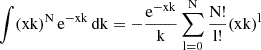$\int {(\mathrm{xk})}^{\mathrm{N}}{\mathrm{e}}^{-\mathrm{xk}}\mathrm{d}\mathrm{k}=-\frac{{\mathrm{e}}^{-\mathrm{xk}}}{\mathrm{k}}\sum _{\mathrm{l}=0}^{\mathrm{N}}\frac{\mathrm{N}!}{\mathrm{l}!}{(\mathrm{xk})}^{\mathrm{l}}$

So the median value can be numerically solved by imposing:

$$\begin{array}{c}\hfill [-{\mathrm{e}}^{-\mathrm{r}\mathrm{\Delta }\mathrm{t}}\sum _{l=0}^{\mathrm{N}}\frac{{(\mathrm{r}\mathrm{\Delta }\mathrm{t})}^l}{\mathrm{l}!}{]}_0^{{\mathrm{r}}_{\mathrm{med}}}=\frac{1}{2}\end{array}$$(B.3)

B.3. Mean

The Poisson mean can be evaluated by considering the expectation value formula:

$$\begin{array}{c}\hfill {\mathrm{r}}_{\mathrm{mean}}=\frac{{\int }_0^{\infty }\mathrm{r}{\mathrm{Q}}_{\mathrm{N};\mathrm{\Delta }\mathrm{t}}(\mathrm{r})\mathrm{dr}}{{\int }_0^{\infty }{\mathrm{Q}}_{\mathrm{N};\mathrm{\Delta }\mathrm{t}}(\mathrm{r})\mathrm{dr}}=\frac{\mathrm{\Delta }{\mathrm{t}}^{\mathrm{N}+1}}{\mathrm{N}!}{\int }_0^{\infty }{\mathrm{r}}^{\mathrm{N}+1}{\mathrm{e}}^{-\mathrm{r}\mathrm{\Delta }\mathrm{t}}\mathrm{dr}\end{array}$$(B.4)

but ${\int }_0^{\infty }{x}^{\mathrm{N}+1}{\mathrm{e}}^{-\mathrm{k}\mathrm{x}}\mathrm{dx}=\frac{(\mathrm{n}+1)!}{{\mathrm{k}}^{\mathrm{N}+2}}$, therefore:

$$\begin{array}{c}\hfill {\mathrm{r}}_{\mathrm{mean}}(\mathrm{N},\mathrm{\Delta }\mathrm{t})=\frac{\mathrm{\Delta }{\mathrm{t}}^{\mathrm{N}+1}}{\mathrm{N}!}\frac{(\mathrm{N}+1)!}{\mathrm{\Delta }{\mathrm{t}}^{\mathrm{N}+2}}=\frac{\mathrm{N}+1}{\mathrm{\Delta }\mathrm{t}}\end{array}$$(B.5)

Appendix C: CL analytical solution

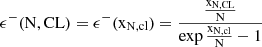
By substituting the expression of ${\mathrm{Q}}_{\mathrm{N},\mathrm{\Delta }\mathrm{t}}(\mathrm{r})$ in Equation 5, the the confidence level condition in conditionin Equation A.6 is:

$$\begin{array}{c}\hfill \frac{\mathrm{\Delta }{\mathrm{t}}^{\mathrm{N}+1}}{\mathrm{N}!}{\int }_{{\mathrm{r}}_{\min }}^{{\mathrm{r}}_{\max }}{(\mathrm{r}\mathrm{\Delta }\mathrm{t})}^{\mathrm{n}}{\mathrm{e}}^{-\mathrm{r}\mathrm{\Delta }\mathrm{t}}\mathrm{dr}=\mathrm{CL}\end{array}$$(C.1)

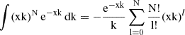but $\int {(\mathrm{xk})}^{\mathrm{N}}{\mathrm{e}}^{-\mathrm{xk}}\mathrm{dk}=-\frac{{\mathrm{e}}^{-\mathrm{xk}}}{\mathrm{k}}\sum _{\mathrm{l}=0}^{\mathrm{N}}\frac{\mathrm{N}!}{\mathrm{l}!}{(\mathrm{xk})}^{\mathrm{l}}$, so we can write the previous equation as:

$$\begin{array}{c}\hfill [{\mathrm{e}}^{-\mathrm{r}\mathrm{\Delta }\mathrm{t}}\sum _{l=0}^{\mathrm{N}}\frac{{(\mathrm{r}\mathrm{\Delta }\mathrm{t})}^l}{\mathrm{l}!}{]}_{{\mathrm{r}}_{\max }}^{{\mathrm{r}}_{\min }}=\mathrm{CL}\end{array}$$(C.2)

By considering the probability condition in Equation A.7 we obtain:

$$\begin{array}{c}\hfill \frac{\mathrm{\Delta }\mathrm{t}}{\mathrm{N}!}{({\mathrm{r}}_{\min }\mathrm{\Delta }\mathrm{t})}^{\mathrm{N}}{\mathrm{e}}^{-{\mathrm{r}}_{\min }\mathrm{\Delta }\mathrm{t}}=\frac{\mathrm{\Delta }\mathrm{t}}{\mathrm{N}!}{({\mathrm{r}}_{\max }\mathrm{\Delta }\mathrm{t})}^{\mathrm{N}}{\mathrm{e}}^{-{\mathrm{r}}_{\max }\mathrm{\Delta }\mathrm{t}}\end{array}$$(C.3)

therefore:

$$\begin{array}{c}\hfill (\frac{{\mathrm{r}}_{\max }}{{\mathrm{r}}_{\min }}{)}^N={\mathrm{e}}^{({\mathrm{r}}_{\max }-{\mathrm{r}}_{\min })\mathrm{\Delta }\mathrm{t}}\end{array}$$(C.4)

C.1. Numerical solution

This 2 equation and 2 variables system can be numerically solved. By defining $x=(r_{\mathit{max}}-r_{\mathit{min}})·\mathrm{\Delta }\mathrm{t}$ and considering the condition above.

$$\begin{array}{c}\hfill {\mathrm{F}}_2(\mathrm{x},\mathrm{y}(\mathrm{x},\mathrm{n}),\mathrm{z}(\mathrm{x},\mathrm{n}),\mathrm{n})=exp(-\mathrm{y})[\sum _{l=0}^{\mathrm{N}}\frac{{\mathrm{y}}^l}{\mathrm{l}!}]-exp(\mathrm{yz})[\sum _{l=0}^{\mathrm{N}}\frac{{(\mathrm{yz})}^l}{\mathrm{l}!}]-\mathrm{CL}\end{array}$$(C.5)

where $\mathrm{y}(\mathrm{x},\mathrm{n})$ is:

$$\begin{array}{c}\hfill \mathrm{y}(\mathrm{x},\mathrm{n})=\frac{\mathrm{x}}{exp(\frac{\mathrm{x}}{\mathrm{n}})-1}\end{array}$$(C.6)

and $\mathrm{z}(\mathrm{x},\mathrm{n})$ is:

$$\begin{array}{c}\hfill \mathrm{z}(\mathrm{x},\mathrm{n})=exp(\frac{\mathrm{x}}{\mathrm{n}})\end{array}$$(C.7)

By imposing ${\mathrm{F}}_2(\mathrm{x},\mathrm{y}(\mathrm{x},\mathrm{n}),\mathrm{z}(\mathrm{x},\mathrm{n}),\mathrm{n})=0$, we can find a numerical solution by solving this equation in the variable x. This yields as a result a x that depends on the number of events considered. The x_n corresponds to the x_N, CL that satisfies the confidence level conditions for a certain number of counts in a given $\mathrm{\Delta }\mathrm{t}$. At this point, we can express the relative confidence interval [ϵ⁻(N, CL), ${ϵ}^{+}(\mathrm{N},\mathrm{CL})$] as

$$\begin{array}{cc}\hfill {ϵ}^{-}(\mathrm{N},\mathrm{CL})& ={ϵ}^{-}({\mathrm{x}}_{\mathrm{N},\mathrm{cl}})=\frac{\frac{{\mathrm{x}}_{\mathrm{N},\mathrm{CL}}}{\mathrm{N}}}{exp\frac{{\mathrm{x}}_{\mathrm{N},\mathrm{cl}}}{\mathrm{N}}-1}\hfill \end{array}$$(C.8)

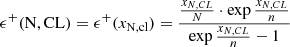$$\begin{array}{cc}\hfill {ϵ}^{+}(\mathrm{N},\mathrm{CL})& ={ϵ}^{+}(x_{\mathrm{N},\mathrm{cl}})=\frac{\frac{x_{N,\mathit{CL}}}{N}·exp\frac{x_{N,\mathit{CL}}}{n}}{exp\frac{x_{N,\mathit{CL}}}{n}-1}\hfill \end{array}$$(C.9)

Therefore the absolute confidence interval [${\mathrm{r}}^{-}(\mathrm{N},\mathrm{CL},\mathrm{\Delta }\mathrm{t})$, ${\mathrm{r}}^{+}(\mathrm{N},\mathrm{CL},\mathrm{\Delta }\mathrm{t})$]

$$\begin{array}{cc}\hfill {\mathrm{r}}^{-}(\mathrm{N},\mathrm{CL},\mathrm{\Delta }\mathrm{t})& ={ϵ}^{-}(\mathrm{N},\mathrm{CL})·{\mathrm{r}}_{\mathrm{mod}}(\mathrm{N},\mathrm{\Delta }\mathrm{t})\hfill \end{array}$$(C.10)

$$\begin{array}{cc}\hfill {\mathrm{r}}^{+}(\mathrm{N},\mathrm{CL},\mathrm{\Delta }\mathrm{t})& ={ϵ}^{+}(\mathrm{N},\mathrm{CL})·{\mathrm{r}}_{\mathrm{mod}}(\mathrm{N},\mathrm{\Delta }\mathrm{t})\hfill \end{array}$$(C.11)

Appendix D: Generalized inversion method analytical solution

The inversion method integral in Equation 12 can be considered as a trapezoidal integral when the rate curve r(t) is a continuous piecewise linear function. By looking at Equation 6 the integral can be rewritten as:

$$\begin{array}{c}\hfill \begin{array}{cc}& \frac{\mathrm{r}(\mathrm{T}\_\mathrm{SIM}[\mathrm{N}])+\mathrm{r}(\mathrm{T}\_\mathrm{SIM}[\mathrm{N}-1])}{2}·\hfill \\ \hfill & ·(\mathrm{T}\_\mathrm{SIM}[\mathrm{N}]-\mathrm{T}\_\mathrm{SIM}[\mathrm{N}-1])=-\ln \{1-\mathrm{RND}(0,1)\}\hfill \end{array}\end{array}$$(D.1)

In the most general case, T_SIM[N − 1] is between two rate points of r(t) as in Figure 6. The rate $\mathrm{r}(\mathrm{T}\_\mathrm{SIM}[\mathrm{N}-1])$ can be linearly extrapolated by considering the intensities of the two rate points r₁ and r₂ that are before and after T_SIM[N − 1]), as well as their respective associated times ${\mathrm{t}}_1$ and ${\mathrm{t}}_2$:

$$\begin{array}{cc}\hfill \mathrm{m}& =\frac{{\mathrm{r}}_2-{\mathrm{r}}_1}{{\mathrm{t}}_2-{\mathrm{t}}_1}\hfill \\ \hfill \mathrm{r}(\mathrm{T}\_\mathrm{SIM}[\mathrm{N}-1])& ={\mathrm{r}}_1+\mathrm{m}·(\mathrm{T}\_\mathrm{SIM}[\mathrm{N}-1]-{\mathrm{t}}_1)\hfill \end{array}$$(D.2)

The same procedure can be performed for the unknown T_SIM[N] from the T_SIM[N − 1] where $\mathrm{r}(\mathrm{T}\_\mathrm{SIM}[\mathrm{N}-1])$ is known. Let us define T_SIM[N − 1] as as $\overline{t}$ and T_SIM[N] as x:

$$\begin{array}{cc}\hfill \mathrm{r}(\mathrm{x})=& {\mathrm{r}}_1+\mathrm{m}·(\mathrm{x}-{\mathrm{t}}_1)\hfill \\ \hfill \frac{\mathrm{r}(\overline{\mathrm{t}})+\mathrm{r}(\mathrm{x})}{2}·(\mathrm{x}-\overline{\mathrm{t}})=& -\ln \{1-\mathrm{RND}(0,1)\}\hfill \\ \hfill \frac{\mathrm{r}(\overline{\mathrm{t}})+{\mathrm{r}}_1+\mathrm{mx}-\mathrm{m}{\mathrm{t}}_1}{2}·(\mathrm{x}-\overline{\mathrm{t}})=& -\ln \{1-\mathrm{RND}(0,1)\}\hfill \end{array}$$(D.3)

The equation can then be rewritten by rearranging the random terms with $\mathrm{ZETA}\equiv -\ln \{1-\mathrm{RND}(0,1)\}$:

$$\begin{array}{c}\hfill \mathrm{m}{\mathrm{x}}^2+\mathrm{x}(\mathrm{r}(\overline{\mathrm{t}})+{\mathrm{r}}_1-\mathrm{m}{\mathrm{t}}_1-\mathrm{m}\overline{\mathrm{t}})+\mathrm{m}{\mathrm{t}}_1\overline{\mathrm{t}}-\overline{\mathrm{t}}\mathrm{r}(\overline{\mathrm{t}})-\overline{\mathrm{t}}{\mathrm{r}}_1-2\mathrm{ZETA}=0\end{array}$$(D.4)

The only possible solution is therefore when $\mathrm{x}>\overline{t}$:

$$\begin{array}{cc}\hfill B& =\mathrm{r}(\overline{t})+r_1-m{\mathrm{t}}_1-m\overline{t}\hfill \\ \hfill C& =\mathrm{m}{\mathrm{t}}_1\overline{t}-\overline{t}\mathrm{r}(\overline{t})-\overline{t}{r}_1-2ZETA\hfill \\ \hfill \mathrm{x}& =\frac{-\mathrm{B}+\sqrt{{\mathrm{B}}^2-4\mathrm{m}\mathrm{C}}}{2\mathrm{m}}\hfill \end{array}$$(D.5)

Appendix E: CCF examples

Figure E.1 from page 12 to 16 shows the GRB considered in the comparison in Figure 10 between DP and MDP method.

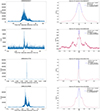Fig. E.1. Right panel: Example CCFs performed between ToA lists (see subsection: 2.4) obtained via the MDP method (see subsection: 4.3). Gaussian fit parameters are highlighted in each plot and fixed for both the MDP and the DP methods testing (see subsection: 5). ToA lists are retrieved from GRB data as observed by the brightest Fermi-GBM detector monitoring the bursts. Left panel: Light curves from the brightest detector, computed using an adaptive bin size of 10 photons per bin.

All Tables

All Figures

	Fig. 1. Normalized Poisson probability function QN, Δt shown as a function of the rate r for N =1 (solid line) and n = 100 (dotted line). The gray areas indicate a confidence level (CL) of 0.68 corresponding to a 1σ CL of a Gaussian distribution.
In the text

Fig. 2. Relative errors (for different CLs) as a function of the observed number of events. The upper and lower limits are expressed in units of the mode rmod = N/Δt (see Appendix B for a detailed computation). The 1, 2 and 3σ confidence levels are respectively associated with 68%, 95% and 99.7%d. The gray lines represent the $\pm 1/\sqrt{\mathrm{N}}$ confidence level as a function of the observed number of events.

In the text

Fig. 3. Top row: Light curves (left and central panels) and corresponding CCF (right panel) obtained using the adaptive rebinning method (10 photons per bin). Middle and bottom rows: Same configuration, but using fixed bin sizes of 1 s and 0.05 s, respectively. In each row, the left panel shows in blue the simulated signal obtained by rebinning the ToA list generated by simulating the theoretical profile shown in orange. The center panel displays the same signal, delayed by 1 s before rebinning. The right panel presents the CCF between the two simulated light curves shown in the left and central panels of the corresponding row.

In the text

	Fig. 4. Light curves of GRB 090820 obtained by counting N =100 photons per bin. The upper panel shows the n1 detector light curve and the lower panel displays the n5 detector light curve.
In the text

	Fig. 5. Upper panel: Cross-correlation function between light curves from the n1 and n5 detector ToA lists, using a variable bin size of 10 photons per bin and a 1 μs resolution. Lower panel: Zoom on the Gaussian fit centroid fluctuation relative to the vertical green dashed line, which indicates the null theoretical delays.
In the text

	Fig. 6. Luminosity curve illustrating the trapezoidal integral in Equation 12. The black point indicates a generic ToA that was just simulated in the previous step, and the red point represents the ToA to be simulated in the current step.
In the text

	Fig. 7. Scheme of the MDP splitting procedure.
In the text

	Fig. 8. Delay distribution is obtained by cross-correlating 100 pairs of ToA lists, derived from the random division of the GRB 180113418 event file. A 1-second delay is injected into one of the ToA lists in each pair.
In the text

	Fig. 9. Delay distribution obtained by applying the MDP method to two of the 200 ToA lists derived from the random division of the GRB 180113418 event file. A 1-second delay is introduced into one ToA list. The MDP procedure is carried out by randomly splitting the initial ToA lists 500 times, resulting in two pools of 1000 light curves each.
In the text

	Fig. 10. Comparison of DP and MDP methods. Left panels: Experimental delays estimated via MC procedures with associated errors shown as vertical error bars. Right panels: Residual distribution for each method in units of sigma.
In the text

Fig. E.1. Right panel: Example CCFs performed between ToA lists (see subsection: 2.4) obtained via the MDP method (see subsection: 4.3). Gaussian fit parameters are highlighted in each plot and fixed for both the MDP and the DP methods testing (see subsection: 5). ToA lists are retrieved from GRB data as observed by the brightest Fermi-GBM detector monitoring the bursts. Left panel: Light curves from the brightest detector, computed using an adaptive bin size of 10 photons per bin.

In the text

References

- Abbott, B. P., Abbott, R., Abbott, T. D., et al. 2017, ApJ, 848, L13 [CrossRef] [Google Scholar]
- Amelino-Camelia, G., Ellis, J., Mavromatos, N. E., Nanopoulos, D. V., & Sarkar, S. 1998, Nature, 393, 763 [Google Scholar]
- Bissaldi, E., von Kienlin, A., Lichti, G., et al. 2009, Exp. Astron., 24, 47 [Google Scholar]
- Burderi, L., Di Salvo, T., Alessandro, R., et al. 2021, Proc. SPIE, 11444, 114444Y [Google Scholar]
- Campana, S., Panagia, N., Lazzati, D., et al. 2008, ApJ, 683, L9 [Google Scholar]
- Castignani, G., Guetta, D., Pian, E., et al. 2014, A&A, 565, A60 [NASA ADS] [CrossRef] [EDP Sciences] [Google Scholar]
- Dado, S., & Dar, A. 2022, ApJ, 940, L4 [NASA ADS] [CrossRef] [Google Scholar]
- D’Avanzo, P. 2015, J. High Energy Astrophys., 7, 73 [CrossRef] [Google Scholar]
- Dekking, F. M., Kraaikamp, C., Lopuhaä, H. P., & Meester, L. E. 2005, The Poisson Process (London: Springer), 167 [Google Scholar]
- Fiore, F., Burderi, L., Lavagna, M., et al. 2020, in Space Telescopes and Instrumentation 2020: Ultraviolet to Gamma Ray, eds. J.-W. A. den Herder, K. Nakazawa, &S. Nikzad, (SPIE) [Google Scholar]
- Frontera, F., Amati, L., Costa, E., et al. 2000, ApJS, 127, 59 [NASA ADS] [CrossRef] [Google Scholar]
- Ghirlanda, G., Nava, L., Salafia, O., et al. 2024, A&A, 689, A175 [NASA ADS] [CrossRef] [EDP Sciences] [Google Scholar]
- Giuliani, A., Mereghetti, S., Fornari, F., et al. 2008, A&A, 491, L25 [NASA ADS] [CrossRef] [EDP Sciences] [Google Scholar]
- Goldstein, A., Veres, P., Burns, E., et al. 2017, ApJ, 848, L14 [CrossRef] [Google Scholar]
- Gompertz, B. P., Levan, A. J., & Tanvir, N. R. 2020, ApJ, 895, 58 [NASA ADS] [CrossRef] [Google Scholar]
- Hurley, K., Pal’shin, V. D., Aptekar, R. L., et al. 2013, ApJS, 207, 39 [Google Scholar]
- Kingman, J. F. C., & Taylor, S. J. 1966, Characteristic Functions (Cambridge University Press), 314 [Google Scholar]
- Klein, R. W., & Roberts, S. D. 1984, Simulation, 43, 193 [Google Scholar]
- Meegan, C., Lichti, G., Bhat, P. N., et al. 2009, ApJ, 702, 791 [Google Scholar]
- Mészáros, P., Fox, D. B., Hanna, C., & Murase, K. 2019, Nat. Rev. Phys., 1, 585 [Google Scholar]
- MIT 2008, Signal Processing– Continuous and Discrete (Department of Mechanical Engineering) [Google Scholar]
- Mochkovitch, R., Hernanz, M., Isern, J., & Martin, X. 1993, Nature, 361, 236 [NASA ADS] [CrossRef] [Google Scholar]
- Park, K. 2018, Fundamentals of Probability and Stochastic Processes with Applications to Communications [Google Scholar]
- Peterson, B. M., Wanders, I., Horne, K., et al. 1998, PASP, 110, 660 [Google Scholar]
- Piran, T. 1999, Phys. Rep., 314, 575 [NASA ADS] [CrossRef] [Google Scholar]
- Piran, T. 2004, Gamma-Ray Bursts as Probes for Quantum Gravity (Springer-Verlag), 351 [Google Scholar]
- Pishro-Nik, H. 2014, Introduction to Probability, Statistics, and Random Processes (Kappa Research, LLC) [Google Scholar]
- Sanna, A., Burderi, L., Di Salvo, T., et al. 2020, in Space Telescopes and Instrumentation 2020: Ultraviolet to Gamma Ray, eds. J.-W. A. den Herder, K. Nakazawa,&S. Nikzad, (SPIE) [Google Scholar]
- Sari, R., Piran, T., & Halpern, J. P. 1999, ApJ, 519, L17 [NASA ADS] [CrossRef] [Google Scholar]
- Savchenko, V., Ferrigno, C., Kuulkers, E., et al. 2017, ApJ, 848, L15 [NASA ADS] [CrossRef] [Google Scholar]
- Tsvetkova, A., Frederiks, D., Golenetskii, S., et al. 2017, ApJ, 850, 161 [NASA ADS] [CrossRef] [Google Scholar]
- von Kienlin, A., Meegan, C. A., Paciesas, W. S., et al. 2020, ApJ, 893, 46 [Google Scholar]
- Wu, S.-W., Xu, D., Zhang, F.-W., & Wei, D.-M. 2012, MNRAS, 423, 2627 [Google Scholar]
- Zajaček, M., Czerny, B., Martínez-Aldama, M. L., & Karas, V. 2019, Astron. Nachr., 340, 577 [CrossRef] [Google Scholar]
- Zhang, Y. H., Celotti, A., Treves, A., et al. 1999, ApJ, 527, 719 [Google Scholar]
- Zhang, S., Zhang, S. N., Lu, F. J., et al. 2018, in Space Telescopes and Instrumentation 2018: Ultraviolet to Gamma Ray, eds. J.-W. A. den Herder, S. Nikzad,&K. Nakazawa, SPIE Conf. Ser., 10699, 106991U [NASA ADS] [Google Scholar]
- Zhang, S.-N., Li, T., Lu, F., et al. 2020, Sci. China: Phys. Mech. Astron., 63, 249502 [Google Scholar]