| Issue |
A&A
Volume 701, September 2025
|
|
|---|---|---|
| Article Number | A29 | |
| Number of page(s) | 24 | |
| Section | Extragalactic astronomy | |
| DOI | https://doi.org/10.1051/0004-6361/202453370 | |
| Published online | 01 September 2025 | |
The interplay between active galactic nuclei and ram pressure stripping: spatially resolved gas-phase abundances of stripped and undisturbed galaxies
1
INAF – Osservatorio Astronomico di Brera, via Brera, 28, 20121 Milano, Italy
2
INAF-Osservatorio Astronomico di Padova, Vicolo Osservatorio 5, 35122 Padova, Italy
3
Instituto de Radioastronomía y Astrofísica, UNAM, Campus Morelia, A.P. 3-72, C.P. 58089, Mexico
4
Department of Physics, Faculty of Science, University of Zagreb, Bijenicka 32, 10 000 Zagreb, Croatia
5
INAF – Osservatorio di Astrofisica e Scienza dello Spazio Bologna, Via Piero Gobetti, 93/3, 40129 Bologna, Italy
6
Dipartimento di Fisica e Astronomia “Augusto Righi”, Università di Bologna, via Piero Gobetti 93/2, I-40129 Bologna, Italy
⋆ Corresponding author: This email address is being protected from spambots. You need JavaScript enabled to view it.
Received:
9
December
2024
Accepted:
25
April
2025
Abstract
Context. It has been reported that the gas-phase oxygen abundance of the circumnuclear regions around supermassive black holes (SMBHs) could be affected by the presence of an active galactic nucleus (AGN). However, there is currently no agreement on the processes behind this effect. Some studies have measured higher metallicities in the nuclear regions of AGN hosts compared to those of star-forming (SF) galaxies, while others have observed the opposite result.
Aims. In this work, we explore whether the interplay between AGN activity and the ram-pressure strippingprocesses of ram-pressure stripping (RPS) acting in the cluster environment could alter the metallicity distributions of nearby (z < 0.07) galaxies.
Methods. We measured the spatially resolved gas-phase oxygen abundances of 10 AGN hosts experiencing RPS from the GASP survey and 52 AGN hosts located in the field (and, thus, undisturbed by RP) drawn from MaNGA DR15. To measure the oxygen abundances in SF and AGN-ionized regions, we present a set of strong emission line (SEL) calibrators obtained through an indirect method. Here, the [O III]/[S II] and [N II]/[S II] line ratios, observed and predicted from CLOUDY photoionization models, were matched using the NEBULABAYES code.
Results. We find that the metallicity gradients of RPS and field AGN generally do not present significant differences within the errors. However, we also find that two two out of the ten ten RP-stripped AGNs display lower oxygen abundances at any given radius than the rest of the AGN sample. Overall, this result highlights the fact that the interplay between AGN and RPS does not seem to play a major role in shaping the metallicity distributions of stripped galaxies within 1.5 times the galaxy’s effective radius (r < 1.5Re); however,but that larger samples are needed to draw more robust conclusions. By adding a control sample of SF galaxies, both experiencing RPS and in the field, we find that the AGN hosts are more metal-enriched than SF galaxies at any given radius, but that the steepness of the gradients in the nuclear regions (r < 0.5Re) is higher in AGN hosts than in SF galaxies. In, particular, AGN hosts show a metal enrichment in the nuclear regions that is about 1.8–2.3 times higher than the enhancement in the disk at r ∼ 1.25Re, regardless of the host galaxy’s stellar mass.
Conclusions. These results favor the hypothesis that AGN activity is the cause behind metal pollution in athe galaxy’s nuclear regions.
Key words: galaxies: abundances / galaxies: active / galaxies: evolution
© The Authors 2025
 Open Access article, published by EDP Sciences, under the terms of the Creative Commons Attribution License (https://creativecommons.org/licenses/by/4.0), which permits unrestricted use, distribution, and reproduction in any medium, provided the original work is properly cited.
This article is published in open access under the Subscribe to Open model. This email address is being protected from spambots. You need JavaScript enabled to view it. to support open access publication.
1. Introduction
Typically, gas-phase metallicity (or, equivalently, abundance) gradients are observed to be negative in spiral galaxies. This is consistent with an inside-out growth of the spiral discs through the accretion of primordial material on a timescale that is a function of the galactocentric distance (e.g., Matteucci 1989; Molla et al. 1996). In this scenario, the gas accumulates and forms the inner disk, where the high density of the gas results in an efficient star formation. The fast gas reprocessing at the galaxy center leads to a population of old, metal-rich stars in an environment of high-metallicity gas. The outer regions are formed later and, therefore, these are characterized by younger, metal-poor stars surrounded by material that is less enrichedless enriched material (e.g., Davé et al. 2011; Gibson et al. 2013; Prantzos & Boissier 1999; Pilkington et al. 2012).
Deviations from the pure inside-out scenario (i.e., from the negative slopes) are also commonly observed (Dekel et al. 2013; Dekel & Mandelker 2014; Tissera et al. 2018; Grisoni et al. 2018). A decrease or a nearly flat distribution in the abundance in the innermost region of discs was first observed by Belley et al. (1992), while the flattening of the metallicity gradient in the nuclear region of the most massive spiral galaxies was also found in other works using CALIFA (e.g., Zinchenko et al. 2016) and MaNGA data (e.g., Belfiore et al. 2017; Khoram & Belfiore 2025; Kewley et al. 2010). Such deviations may originate from the effects of other mechanisms, aside from the in situ production through stellar processes, such as a loss of metals through outflows in the form of galactic winds (Heckman et al. 2000; Veilleux et al. 2017; Tremonti et al. 2007; Feruglio et al. 2010), the transport of pristine gas through gas inflows into the galaxy from the circumgalactic (CGM) and the intergalactic medium (IGM, Prochaska et al. 2017; Tumlinson et al. 2017), or an exchange between the halo and the galaxy due to interacting processes such as mergers (e.g., Barnes et al. 1991, 1996) and ram-pressure stripping (RPS) (Hughes et al. 2013; Franchetto et al. 2020, 2021; Khoram et al. 2024). Another process that can alter the distribution of metals is the activity of an active galactic nucleus (AGN), even if there are discrepant views on how this occurs. The nuclear regions of AGN hosts have been observed to be either metal-rich (e.g., Thomas et al. 2019; Peluso et al. 2023) or metal-poor (e.g., Storchi-Bergmann et al. 1998; Armah et al. 2023) with respect to those of SF galaxies. A possible interpretation to explain a lower metallicity around the nuclear supermassive black hole (SMBH) is the accretion of metal-poor gas that feeds the AGN (Storchi-Bergmann & Schnorr-Müller 2019). On the other hand, the metal enrichment due to AGN could be due to either an in situ top-heavy initial mass function (IMF) in the accretion disk around the SMBH (e.g., Nayakshin & Sunyaev 2005) or dust destruction in the broad line region (BLR), which releases metals into the ISM (Maiolino & Mannucci 2019). AGN-driven outflows may also contribute by re-distributing the gas from the BLR on parsec (pc) scales (e.g., D’Odorico et al. 2004) to the narrow-line region (NLR). Indeed, many works have shown that AGN-driven outflows are typically not as effective as expected in expelling metals from the galaxy disk (see also Bischetti et al. 2019; Feruglio et al. 2017; Veilleux et al. 2017) and, despite the high velocities involved, most of the gas does not escape the disk (Arribas et al. 2014; Swinbank et al. 2019). On the other hand, ionized gas outflows detected through optical emission lines are frequently observed in the NLR (e.g., Veilleux & Osterbrock 1987; Unger et al. 1987; Pogge 1988).
A small number of attempts have been made to measure the spatially resolved abundances in AGN host galaxies. Thomas et al. (2018a) studied the spatially resolved abundances in the extended NLR (ENLR) in four “pure Seyfert” galaxies from the Siding Spring Southern Seyfert Spectroscopic Snapshot Survey (S7, Dopita et al. 2015, z < 0.02, i.e., reaching a spatial resolution up to 408 pc). They found a steep inverse or flat metallicity gradients depending on the single-case, indicative of heterogeneity in the mechanisms shaping the observed distributions. Amiri et al. (2024) found a positive gradient in the Seyfert NGC 7130 but with the lowest value in the most central region dominated by the AGN ionization. A set of MUSE data were usedable to resolve the NLR due to the vicinity of the source (z = 0.016), which allowed to achievefor spatial resolutions of ∼0.3 kpc to be achieved. Going beyond a single case study and exploiting larger samples, Nascimento et al. (2022) measured the abundance gradients in a sample of Seyfert from the inner AGN-dominated regions up to the outer star-forming (SF) regions, exploring integral-field spectroscopy (IFS) data from the MaNGA DR15 survey (Bundy 2015, z < 0.15). These maps were characterized by a spatial resolution of 1 − 4 kpc. They found differences of 0.16 to 0.30 dex between the abundances in the nucleus and the HII regions of the galactic disk.
In this work, we isolate the AGN hosts in clusters and in the field to explore the effect of the environment on the metallicity gradients. So far, the role of the RPS in driving the evolution of galaxies, including its AGN activity, has been investigated by a large number of both observational and theoretical studies. Many observational works agree that the RPS initially enhances the SFR in the surviving disk (Gavazzi et al. 1995, 2001; Consolandi et al. 2017; Vulcani et al. 2018, 2020). It has been argued that the increased SF may result from an increased density linked to the compression of the gas in the leading side of the disk (Tomicic et al. 2018). Vulcani et al. (2018) measured the SFR-M* of 42 RP-stripped galaxies, finding a systematic average enhancement (0.2 dex) at any given mass with respect to a control sample of 32 field and undisturbed cluster galaxies. These galaxies were drawn from the GAs Stripping Phenomena in galaxies with MUSE (GASP, Poggianti et al. 2017) program, which is a MUSE large program aimed at studying the gas removal processes in massive (logM*/M⊙ ≥ 9.0) galaxies in different environments. Alongside an increased SFR, the GASP sample also showed an enhanced AGN fraction (∼46%) with respect to field galaxies (∼28%) (Poggianti et al. 2017; Peluso et al. 2022), indicative of a starburst-AGN activity connection (Matsuoka et al. 2013) in these objects. The galaxies used to compute the above fractions span the mass range of log(M*/M⊙)≥10.0, typical of AGN hosts (e.g., Kauffmann et al. 2003). The AGN fraction increases as a function of the tail’s length, as indeed the chance for a jellyfish to host an AGN is 56%, as opposed to 33% in galaxies at earlier or later stages of the stripping (Peluso et al. 2022). To explain this result, both hydrodynamical and cosmological simulations have found growing evidence of angular moment loss induced by the ICM-ISM interaction, which pushes inflows of gas towards the galaxy centers (Akerman et al. 2023; Schulz & Struck 2001; Tonnesen et al. 2009; Ramos-Martínez et al. 2018) and may light up or enhance the AGN activity. In particular, Ricarte et al. (2020) found that the black hole accretion rate (BHAR) increases strongly and corresponds to the SFR’s peak, when the RPS intensity reaches its maximum. These results suggest a possible link between the increased star formation and AGN activity observed in the GASP sample, which is composed of RP-stripped galaxies hosted by clusters spanning a wide range of velocity dispersions, from Fornax to Coma-like (Poggianti et al. 2025).
However, it is worth mentioning that other works, focusing on single clusters, have reported contrasting results and, thus, hampering the ability to draw more robust conclusions. Roman-Oliveira et al. (2018) have shown that only 5 over 70 jellyfish with stellar mass logM*/M⊙ ≥ 9.0 seem to show AGN activity in the A901/2 cluster at z = 0.165 (see also Boselli et al. 2022). However, as also shown by simulations, the period of activity of the SMBH is expected to be relatively short in the whole life cycle of a galaxy undergoing RPS (Ricarte et al. 2020). Indeed, after the intensity peak of the RPS, both SF and the BHAR decrease rapidly.
To explore the metal distribution in the case of an AGN-RPS interplay, as described above, spatially resolved abundance gradients of a large sample of RP-stripped galaxies are needed, as well as gradients from a control sample of non-stripped AGN hosts to perform a comparison with the RPS sample. The use of IFS data allows us to retrieve the metallicity gradients necessary to investigate the metal production and pollution in these objects in detail and to disentangle ionization from the AGN or the stars. Optical spectroscopy, in particular, is needed to perform measurements of the oxygen abundance, which tends to happencan be done via a direct method (also called aTe-method) involving auroral lines (such as [O III]λ4363, see, e.g., Dors et al. 2020b) or an indirect method involving photoionization models (see, e.g., Thomas et al. 2019). The direct Te-method has been widely adopted to measure abundances in HII and AGN-ionized regions (e.g., Dors et al. 2020a). However, although AGNs have a high-ionization degree, their high (e.g., Groves et al. 2006) metallicity leads to faint auroral lines (such as the [O III] λ4363), hampering the use of the Te-method. Some works (e.g., Thomas et al. 2019; Pérez-Díaz et al. 2021) have developed AGN and stellar photoionization models using the same method and compared observed and predicted line ratios by making use of the Bayesian inference with codes such as NEBULABAYES (Thomas et al. 2018a) or HII-CHI-MISTRY (Pérez-Montero 2014; Pérez-Montero et al. 2019). Strong emission-line (SEL) calibrators for the NLR have been derived through photoionization models (e.g., Carvalho et al. 2020; Storchi-Bergmann et al. 1998) or the direct method (Flury & Moran 2020; Dors 2021). However, the SEL calibrators obtained by measuring the abundances with the same method and using the same set of measurements in case of ionization from star formation and AGNs are not yet available in the literature.
In this paper, we present a set of SEL calibrators to measure the oxygen abundance in HII (or equivalently, SF), AGN, and AGN+HII regions classified by the Baldwin, Philiphs, and Telervich (BPT, Baldwin et al. 1981) diagram, involving the [N II]/Hα and [O III]/Hβ ratios, also called [N II]-BPT. Exploiting these calibrators, we analyzed the spatially resolved oxygen abundances of stripped and undisturbed galaxies using IFS data from the GASP and the Mapping Nearby Galaxies at Apache Point Observatory (MaNGA, Bundy 2015) surveys. Our sample comprises galaxies with and without AGN activity, as evident from the BPT classification. We isolated stripped AGN and nonstripped AGN to explore whether the interplay between RPS and AGN activity affects the metallicity distributions. In this study, which follows up on our previous work (Peluso et al. 2023), where we observed enhanced nuclear metallicity in AGN hosts compared to SF galaxies, we investigate the metal abundances at various galactocentric distances within both AGN and SF galaxies. Our goal is to determine whether the increased metallicity in AGN hosts is limited to the nuclear regions, indicating that it results directly from AGN activity.Alternatively, we consider whether it extends throughout the entire galaxy disks. If the latter is true, it would indicate that the observed enhancement in metallicity may be influenced by other factors, such as the galaxy’s star formation history (SFH).
Sections are structured as follows: the observational dataset used for the analysis is described in Sect. 2, followed by Sect. 3, where we present the SEL calibrators. Section 4 gives our main results. In Sect. 5, we discuss the possible secondary dependence of the results linked to the method used to measure the metallicity or the galaxy’s properties characterizing the sample. Finally, in Sect. 6, we present our summary and conclusions.
We adopt the Chabrier (2003) initial mass function in the mass range of 0.1–100 M⊙. We assume a standard ΛCDM cosmology with Ωm = 0.3, ΩΛ = 0.7 and H0 = 70 km s−1 Mpc−1. Throughout this work, we adopt 12 + log(O/H) = 8.69 as the solar oxygen abundance (Asplund et al. 2009).
2. Datasets and galaxy samples
As in Peluso et al. (2023) (P23, hereafter), this paper is based on galaxies selected from the GASP (Poggianti et al. 2017) and MaNGA (Bundy 2015) surveys. The former sample allows us to characterize galaxies located in clusters and experiencing RPS, and the latter to define a field sample (FS) to study galaxies not disturbed by environmental effects. In this way, we can understand the influence of the RPS phenomenon on the galaxy’s properties. Since we are also interested in focusing on the role of AGN activity in regulating the metal content in galaxies and in a more detailed, particularly, in the study of the interplay between RPS and AGN activity, in both samples we separate galaxies hosting AGN activity from those dominated by star formation within the nuclear regions. In both samples, we selected galaxies with a high specific star formation rate (sSFR > 10−11 M⊙/yr) and with a late-type morphology according to their optical emission. This first selection leads us to four samples: AGN-RPS, AGN-FS, SF-RPS, and SF-FS, which are described in detail below.
2.1. RPS sample
The RP-stripped galaxies are selected from GASP. The program targeted 114 galaxies in the redshift range 0.04 < z < 0.07 and mostly located in clusters. Observations were carried out with the MUSE spectrograph, which covers the wavelength range 4650–9300 Å and have a seeing-limited spatial resolution of ∼1 kpc. The data, reduced with the MUSE pipeline (Bacon et al. 2010), were first corrected for extinction caused by our own Galaxy, estimated at the position of each galaxy (Schlafly & Finkbeiner 2010) using the extinction law from Cardelli et al. (1989). Next, the emission lines were fitted with the code KUBEVIZ (Fossati et al. 2016) from the continuum-subtracted and extinction-corrected MUSE spectrum, as described in Poggianti et al. (2017). Finally, the flux measurements were further corrected for extinction by dust internal to the host galaxy. The correction is derived from the Balmer decrement at each spatial element location adopting the Cardelli et al. (1989) extinction law and assuming an intrinsic Balmer decrement  , appropriate for an electron density ne = 100 cm−3 and electron temperature Te = 104 K (Osterbrock 2006). Integrated galaxy global properties such as inclination, position angle, and effective radius (Re) are taken from Franchetto et al. (2020), who measured these quantities by means of I-band MUSE photometry. In particular, the effective radius, Re, was computed from the luminosity growth curve, L(R), of the galaxies, obtained by trapezoidal integration of their surface brightness profiles. Stellar masses, which range from logM*/M⊙ = 9.0 to logM*/M⊙ = 11.5, are taken from Vulcani et al. (2018) and are computed assuming a Chabrier (2003) IMF using the SINOPSIS spectrophotometric code (Fritz et al. 2017). These quantities are obtained by summing the values of all of the spaxels belonging to the galaxy disk, as defined in Gullieuszik et al. (2020). To quantify the effect of the stripping, we selected galaxies at least in an early stage of the stripping (namely, JType ≥ 0.5) where JType is a number ranging from 0 to 4 quantifying the visual evidence for stripping signatures (see Poggianti et al. submitted for further details on the definition of JType).
We selected 51 galaxies located in clusters that show signs of stripping. Among them, 11 host an AGN according to the spatially resolved BPT classification (i.e., AGN-RPS, see also Peluso et al. 2022) with the [N II]/Hα versus [O III]/Hβ diagnostic ([N II]-BPT, Baldwin et al. 1981). JO36 is an obscured AGN detected by Chandra as a point-like X-ray source (Fritz et al. 2017), but not directly identified using BPT diagrams due to strong dust absorption and for this reason was not included in the AGN-RPS sample. The remaining 39/51 galaxies are dominated by SF emission. Since Franchetto et al. (2020) could not retrieve the structural parameters for 4 out of the 39 from their I-band photometry, we ended up with an SF-RPS sample of 35 galaxies with log(M*/M⊙)≥9.0. All the AGN hosts have stellar masses log(M*/M⊙)≥10.5, while only 6/35 SF galaxies are in this mass regime.
2.2. Field sample
We selected galaxies located in the field from the MaNGA (Mapping Nearby Galaxies at Apache Point Observatory; Bundy 2015) survey, which is an integral-field spectroscopic survey using the BOSS Spectrograph (Smee et al. 2013) mounted at the 2.5 m Sloan Digital Sky Survey (SDSS) telescope (Gunn et al. 2006) and, in particular, we exploited the MaNGA Data Release 15 (DR15; Bundy 2015). The spectral coverage extends from 3600 to 10 300 Å.
To ensure that galaxies are not affected by RPS, we consider only galaxies located in halo masses lower than Mhalo < 1013 M⊙, according to the Tempel et al. (2014) environmental catalog. We use the online tool MARVIN1 (Cherinka et al. 2019) to download the elliptical radius and azimuth (spx_ellcoo), and the emission line fluxes (gflux). The de-projected coordinates are computed using the ellipticity (ϵ = 1 − b/a) and position angle (θ) measured from the r-band surface brightness. The same emission line fluxes are drawn from the drpall-v2_4_3 and have S/N > 1.5, which is the value typically adopted in MaNGA (Belfiore et al. 2019b). Emission lines are fitted with a Gaussian function and are corrected for stellar absorption since the Data Analysis Pipeline (DAP; Westfall et al. 2019; Belfiore et al. 2019b) simultaneously fits the continuum and emission lines with the latest version of the pPXF software package (Cappellari 2017). All lines are also corrected for Galactic extinction, using the Schlegel et al. (1998) maps (Westfall et al. 2019) and the reddening law of O’Donnell (1994). Following the same approach used in GASP, we corrected the emission lines for the host galaxy dust attenuation using the Cardelli et al. (1989) law. We discarded spaxels with S/N < 3 for any of the emission lines Hβ, [O III] λ5007, Hα, [N II] λ6584, [S II] λ6716, and [S II] λ6731. We selected 429 galaxies located at redshift below z < 0.04, which corresponds to a spatial resolution of ∼1 kpc inside the MaNGA PSF of 2.5′′ (Law et al. 2016). These are part of the Primary+Color-Enhanced (or Primary+) sample (Bundy 2015) and, thus, they display a smooth distribution in redshift (see Figure 8 in Bundy 2015). These galaxies are also part of the Pace et al. (2019a,b) catalog, from which we extract an estimate of the total stellar mass. Pace et al. (2019a,b) make use of the principal component analysis (PCA) to compute the stellar mass within the FoV of MaNGA, which covers the galaxies of the Primary+ sample up to 1.5 effective radius (Re), and of the color-mass relation by Bell et al. (2001) to compute the stellar mass outside the MaNGA FoV, thanks to the NASA Sloan Atlas (NASA Blanton et al. 2011) colors and magnitudes. As already discussed in P23, in this way, we checked that stellar masses from MaNGA and GASP are estimated similarly and coherently, and that they are not affected by systematic effects (e.g., different data reduction and instruments) related to the use of two surveys. The final sample spans the stellar mass range 9.0 ≤ log(M*/M⊙)≤11.3. Among the 429 galaxies, 52 are Seyfert/LINER (i.e., AGN-FS) according to the [N II]-BPT classification. Then,Instead, 377 galaxies are instead classified as star-forming and constitute to the SF-FS (see also P23). AGN hosts have stellar masses of log(M*/M⊙)≥10.5, while 78 out of the 377 SF galaxies exceed this threshold.
3. Method
3.1. Photoionization models and the code NEBULABAYES
We used an indirect method to compute the gas-phase oxygen abundances. As described in detail in P23, we generated photoionization models with the code CLOUDY v17.02 (Ferland et al. 2017) assuming the gas to be ionized by radiation coming from stars (HII models, hereafter) or AGN (AGN models, hereafter). More details are given in the online material2. We assumed a gas density of  , stellar age t* = 4 Myr, and a simple power law to model the AGN continuum, with a slope from the infrared to X-ray wavelengths equal to α = −2.0. The free parameters are the ionization parameter (logU) and the gas-phase metallicity (logZ, or equivalently, oxygen abundance 12 + logO/H).
To compute the metallicity in composite (AGN+SF) regions, we mixed the HII and AGN models viausing the expression:
 (1)
(1)
where R is the flux of the reference line,( namely, Hβ), thus RAGN is the Hβ flux that arises from the AGN and RHII is the Hβ flux that arises from the HII regions. In other words, the parameter ‘AGN fraction’ (fAGN) is driving the mixing and this is defined as the fraction of Hβ flux arising from the AGN with respect to the total (HII regions+AGN) Hβ flux. For further details on the HII, composite, and AGN models, we refer to Sections 3.1, 3.2, and 3.3 in P23.
Then, we used the Bayesian code NEBULABAYES (Thomas et al. 2018a,b, 2019) to find the best model that reproduces the observed emission. More specifically, the code takes as input a set of observed line ratios, and corresponding uncertainties, to return the parameters of photoionization models (e.g., metallicity, ionization parameter, gas density, etc.) that best match the observed emission. To do so, the code computes the posterior probability distribution function (PDF) by multiplying the so-called likelihood with a prior. The likelihood is the probability that a particular set of model parameter values are truly representative of the observed line ratios (for further details on the Bayesian calculation, see Thomas et al. 2018a). The prior, which is a function assigned by hand, was chosen to be uniform, since the combination of lines used in input to the code is already sufficient to give a constraint on the free parameters. Finally, the “best model” is the point in the parameter space that maximizes the posterior PDF.
As input, we used the observed lines [O III]λ5007 (hereafter, [O III]) and [N II]λ6584 (hereafter, [N II]) divided by a reference line, which in our case was the sulfur duplet [S II]λλ(6716+6731) ([S II], hereafter). This essentially translates into comparing predicted and observed [O III]/[S II]and [N II]/[S II]ratios (see also P23). As shown in Figure 1 of P23, these two-line ratios, coupled together, work excellently in breaking any degeneracy between logU and logZ, for a fixed gas density (e.g.,  ).
).
3.2. Metallicity calibrators in SF and AGN-ionized regions
Despite the fact that the NEBULABAYES analysis represents an excellent technique for measuring metallicity in a robust way, this routine is relatively expensive in terms of time and computational power. Because of this, we derived three simple equations: one to derive the oxygen abundance in regions ionized by stars, (SF calibrator), one in the AGN-ionized regions (AGN calibrator), and one in the composite regions (COMP calibrator). Computing the abundances with these equations, which are a linear combination of the observed [O III]/[S II] and [N II]/[S II] line ratios, reduces the computational time from hours to minutes. We obtained them by fitting the relation between 12 + log O/H, as computed by NEBULABAYES and the [O III]/[S II] and [N II]/[S II] line ratios observed in HII, AGN, and HII+AGN regions (in the [N II]-BPT). To obtain the COMP calibrator, we considered only line ratios inside the “composite” spaxels, in which the photoionization models predict the parameter fAGN to be 0.2 because the majority (85%) of the composite spaxels are characterized by this value of fAGN. The 3D surfaces (shown in Figure 1) are fitted with a least-square method and can be described by the following equations:
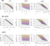 |
Fig. 1. Surfaces of 12 + log O/H versus x ≡ log([N II]/[S II]) and y ≡ log[O III]/[S II], as described by the SF calibrator or Eq. (2) (top panels), COMP calibrator or Eq. (4) (center panels) and AGN calibrator or Eq. (3) (bottom panels), rotated of an angle of 0° (right), 90° (center) and 45° (left). The surfaces are obtained by fitting with a least-squared method the observed [O III]/[S II] and [N II]/[S II] line ratios and the 12 + log O/H computed with NEBULABAYES inside the SF spaxels of all the samples, and the composite and AGN spaxels in the AGN-RPS and AGN-FS. Cells are color-coded according to the value of 12 + log O/H. |
 (2)
(2)
 (3)
(3)
 (4)
(4)
where x ≡ log ([N II]/[S II]) and y ≡ log ([O III]/[S II]). The linear correlation in the 3D plane between the line ratios and the oxygen abundance is applicable up to 12 + log O/H = 8.2, whereas it disappears for lower metallicities. Thus, the validity range is set to be 12 + log O/H > 8.2. These calibrators (hereafter, the P24 calibrators) are both easier to apply and considerably reduce the computational time needed to obtain spatially resolved maps. Henceforth we use the values obtained by Eqs. (1), (2), and (3) to describe metallicities in the various regions.
Figure 2 demonstrates that the surfaces of Eqs. (2), (3), and (4) successfully reproduce the spaxel-by-spaxel predictions by photoionization models. The distribution of the difference  between the abundances computed with the calibrators (12 + log O/HCalib) and with photo-ionization models coupled with NEBULABAYES (12 + log O/HNeb) is plotted versus the values of 12 + log O/HNeb. Depending on the value of 12 + log O/HNeb,
  peaks between 0.02 dex and −0.02 dex in the SF spaxels, while the median μ is constantly ∼0.0 dex at any 12 + log O/HNeb in the AGN and composite spaxels. The yellow histograms in the top panels show that the median value of
  (μ) (over all the values of 12 + log O/HNeb) is 0.0 in all three panels, with a scatter of ±0.01, ±0.009 and ±0.008 dex given by the 25th and 75th percentiles for the SF, AGN+SF, and AGN spaxels3. Gray arrows point out that the error computed by NEBULABAYES for the metallicity estimates (ϵ, which is the maximum between the 16th and 84th percentiles of the posterior PDF) is a factor that is about three times higher than the maximum difference. Thus, the uncertainty on the metallicity estimates remains the one associated to the photo-ionization models, as indeed the error introduced by the linear fitting is negligible. Only one galaxy, JW100 (part of the AGN-RPS sample) shows significant deviations from the calibrators’ planes (μ > 0.1 dex). This galaxy is also notably characterized by peculiar ISM conditions, as deduced by the high X-ray luminosity in the tail (e.g., ten times higher than other tails in RP stripped galaxies, see Sun et al. 2021; Poggianti et al. 2019) and the still-unclear excess of [O I]λ6300 emission (which is still unclear) with respect to what is typically observed in extra-nuclear HII regions (Poggianti et al. 2019). Because of these reasons, the galaxy was discarded from the AGN-RPS sample.
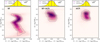 |
Fig. 2. 12 + log O/H computed by NEBULABAYES (12 + log O/HNeb) versus the difference |


3.3. Metallicity gradients and slopes
Spatially resolved maps (with a resolution of ∼1 kpc) of the oxygen abundance are obtained by making use of the SF, COMP, and AGN calibrators (presented in Sect. 3.2) applied to spaxels classified accordingly to the [N II]-BPT.
Once the metallicities are computed for any given spaxel, we divide each galaxy into concentric annuli with width 0.3Re, except for the first central annulus having an outer radius of r = 0.5Re. We chose this aperture as this is always larger than the PSF (e.g., aperture with diameter d ∼2.5″ in MaNGA, and d ∼ 1″ in GASP) and therefore includes a well-resolved galactic region. To obtain the metallicity gradients, we computed the median value of 12 + log O/H of all the spaxels (AGN, composite, SF) inside each annulus and the corresponding 25th and 75th percentiles of the 12 + log O/H distribution. We set a threshold on the minimum number of spaxels used to compute the medians and errors, which is Nth = 10 spaxels. Finally, we plotted the median values of 12 + log O/H versus the mean value of R/Re inside a given annulus. The outermost radius (rout) of the last annulus was set to be r ∼ 2.5Re. However, in some cases the MaNGA data cover the galaxy disks only up to a radius R ∼ 1.5Re or R ∼ 2.2Re (see Bundy 2015, for details). For this reason, to consistently compare the results among all the galaxies of the different samples, we considered abundances up to rout ∼ 1.5Re, which is the maximum distance covered in all galaxies.
To quantify the abundance variation throughout the galaxy, we define the slope Δα of the radial profile as:
 (5)
(5)
with δ (O/H)=12 + log O/Hr = 1Re − 12 + log O/Hr < 0.5Re and δR = 1Re. We computed the slopes only within the galaxy’s optical radius (R < 1Re), which helps us avoid the flattening effect that is typically observed at very large galactocentric radii (R > 2Re) that is indicative of galactic outskirts having accreted pre-enriched material (see Maiolino & Mannucci 2019; Franchetto et al. 2021).
4. Results
4.1. How the AGN-RPS interplay affects the metallicity
The complete atlas of the spatially resolved gas-phase metallicity abundances of 477 galaxies in our samples has been published online4. As an example, we show in Figure 3 (in the first and second rows), the metallicity maps (on the left) and gradients (on the right) of the RP-stripped galaxy JO49 hosting an AGN (logM* = 10.68, z = 0.0451) and the SF RP stripped galaxy JO93 (logM* = 10.54, z = 0.037), which does not show signs of AGN activity in its center. We picked these two galaxies since they have similar stellar mass. Both galaxies show steep and negative gradients. JO93 shows a plateau reaching the value 12 + log (O/H) ∼ 9.05 inside the region with a radius of r ∼ 0.5Re. JO49, instead, shows a plume of points in the same region, which is in this case dominated by the AGN emission according to the BPT. As a consequence, the measured 12 + log (O/H) is 9.2. We retrieved qualitatively similar gradients in the field, as shown in third and fourth rows of Fig. 3 for the AGN galaxy ‘8311-6104’ (logM* = 10.67, z = 0.027) and the SF galaxy ‘8329-12701’ (logM* = 10.99, z = 0.035). Again, the gradient of the SF galaxy flattens at r < 0.5Re around the value 12 + log (O/H) ∼ 9.0, while the abundances of the AGN galaxy increases steeply up to 12 + log (O/H) ∼ 9.2 in the same region, which is dominated by AGN activity. We note that in the SF galaxy 8329-12701, there is no detectable line emission in the outermost annuli; because of this, the gradient on the left panel shows the abundances up to r ∼ 1.5 Re. Similarly, the gradient of 8311-6104 extends up to the radius ∼2.2 R/Re, because the last annulus (rin ∼ 2.3 Re and rout ∼ 2.5 Re) contains less than 10fewer than ten spaxels, which is the minimum threshold to compute the median 12 + log O/H.
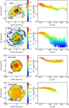 |
Fig. 3. From top to bottom: Metallicity maps (left panels) and metallicity gradients (right panels) of the cluster-AGN host galaxy (JO49, logM* = 10.68, z = 0.0451), cluster-SF galaxy (JO93, logM* = 10.54, z = 0.037), field-AGN galaxy (‘8311-6104’, logM* = 10.67, z = 0.027), and the field-SF galaxy (‘8329-12701’, logM* = 10.99, z = 0.035), shown from top to bottom. On the left: Black contours are overplotted on the metallicity map to divide the SF, composite, and AGN-like regions, as classified by the [N II]– BPT. The gray dotted ellipses are the annuli that cover the galaxy up to Re ∼ 2.5, proceeding with a step of 0.3 dex, except for the central annulus, which has an inner radius of rin = 0Re and an outer radius of rout = 0.5Re. Inside each annulus, the median value of the 12 + log O/H distribution is computed, along with the 25th and 75th percentiles, considering all the 12 + log O/H values inside the SF, composite, and AGN spaxels. On the right: Metallicity profile (gray line) is, obtained by joining the median values of 12 + log O/H of each annulus, plotted versus the mean value of R/Re inside a given annulus, and t(gray line). The shaded area that covers the range of 12 + log O/H values within the 25th and 75th percentiles. In both panels, the color coding is set according to the value of 12 + log O/H, ranging from 8.0 to 9.4. |
In the following, we consider the metal distribution of all the AGN in our sample, including both those hosted by ram-pressure stripped and undisturbed galaxies. We compare the metallicity as a function of the galactic radius of the AGN-RPS and AGN-FS galaxies. Figure 4 shows the distribution of the RP-stripped AGN (red circles) and non-RP-stripped AGN (dark red triangles) galaxies in diagrams comparing the abundances inside concentric annuli at different galactocentric distances. We use the term “nuclear metallicity” to indicate the quantity 12 + log O/Hr < 0.5Re, which is the median metallicity within the nuclear annulus with r < 0.5Re and we use “disk metallicity” to indicate the abundance 12 + log O/Hr = 1Re, which is the median metallicity measured between r = 0.9Re and r = 1.1Re.
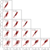 |
Fig. 4. Diagram comparing each pair of metallicities obtained at different radii for AGN-RPS(red circles) and AGN-FS (dark red triangles). The lines show the probability density distribution evaluated using KDE. The comparison is performed among abundances computed at r < 0.5Re, r = 0.6Re, r = 0.8Re, r = 1.2Re, and r = 1.4Re. |
A 2D Kolmogorov Smirnov (2 KS) test, run pairwise in the AGN-RPS and AGN-FS samples of each diagram, was not able to robustly establish whether the distributions are drawn from different parent samples. We observe that the correlation in Figure 4 between the metallicity in the two most external annuli (e.g., 12 + log O/Hr = 1.2Re versus 12 + log O/Hr = 1.4Re) is tight; this is also the case with the correlation between 12 + log O/Hr = 1Re and 12 + log O/Hr = 0.8Re in both the AGN-FS and AGN-RPS. On the other side, the panels in the bottom row show that distributions tend to be more scattered when comparing the metallicity in the nuclear region (R < 0.5Re) with those in the outermost annuli. This is indicative of a significant variation of the slopes. In particular, we show Δα as a function of the nuclear metallicity at r < 0.5Re (12 + log O/Hr < 0.5Re) in Figure 5 (left panel). We note, first of all, that the slopes are all negative, ranging between [−0.3,0.0] dex  . According to a Kendall τ test (similar to a Spearman test, but better suited in cases of small sample sizes), there is a strong correlation between Δα and 12 + log O/Hr < 0.5Re among the AGN-RPS galaxies, with a coefficient kτAGN = −0.73 (p-value = 0.8 × 10⁻³), while the AGN-FS does not show a significant correlation with the disk’s metallicity within r < 0.5Re (spAGN = −0.37, p-value = 9 × 10⁻⁵).
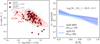 |
Fig. 5. Left: Gradient’s slope (Δα) as a function of the nuclear metallicity. The legend shows the Kendall τ test’s coefficients revealing that the slopes seem to correlate with the nuclear metallicity only in the AGN-RPS,(kτAGN = −0.73). Right: Median oxygen abundance of the AGN-RPS galaxies (purple dotted line) and AGN-FS galaxies (blue continuous line), as a function of the galactic radius, spanning a mass range of 10.5 ≤ logM*/M⊙ ≤ 11.5. The shaded areas cover the 25th and 75th percentiles of the abundance distribution inside each annulus. |
Two galaxies from the AGN-RPS sample, JO206 and JO171, stand out from the main distribution showing significantly flatter slopes at fixed nuclear metallicity, which also displays lower metallicities at any given radius as visible from Figure 4. These two galaxies were also outliers in P23, being the only two AGNs lying below the SF mass-metallicity relation (SF MZR, see Figure 7 of the paper). We describe some of the main properties of these outliers in Appendix A, even though a full understanding of the reasons behind their peculiar metal distributions is beyond the scope of this work. Looking beyond JO206 and JO171, the correlation in the AGN-RPS sample stands with a coefficient of kτAGN = −0.71 (p-value = 0.01). Interestingly, we also observe a significant scatter in four field AGN showing steeper gradients at a fixed value of 12 + log O/Hr < 0.5Re than the rest of the AGN sample. In Appendix A, we show that these galaxies also have steeper slopes than those with the same nuclear luminosity and stellar masses. According to the 2KS test, there is no significant difference in the distribution of the gradients in AGN-RPS and AGN-FS galaxies. Overall, the RPS seems to play a negligible effect in the metallicity gradients in our AGN sample. However, we stress that larger samples of RP-stripped galaxies hosting AGN activity are highly required to study the AGN-RPS connection further. As an ultimate check, we compute the median abundances at a given R/Re among the 10 AGN-RPS and 52 AGN-FS galaxies (shown in the right panel of Figure 5) and we observe that the maximum difference is ∼0.05 dex, well below the errors of ∼0.2 dex. In conclusion, RPS does not play a role in regulating the metal content in AGN hosts as the metallicities at different radii do not differ from those in the field in the same stellar mass range.
4.2. Oxygen abundances of AGN hosts and SF galaxies
In this section, we look to compare the abundances in SF and AGN host galaxies. For completeness, we checked that the metallicity gradients of the stripped and non-stripped SF galaxies were also consistent (as for the AGN hosts; see Sect. 4) within the errorbars, across a very wide stellar mass range (9.0 ≤ logM*/M⊙ ≤ 11).
For the reasons above, we chose not to make any further distinctions between field and RP-stripped galaxies; instead, we set our focus on the comparison between AGN host galaxies versus pure SF galaxies without AGN activity. Since AGN hosts have stellar masses logM*/M⊙ ≥ 10.5, we selected the 83/412 SF galaxies from the SF-FS+SF-RPS samples above the same threshold.
Figure 6 shows the median oxygen abundance as a function of the galactocentric distance (expressed in units of effective radius, Re) of AGN (dotted lines) and SF (continuous lines) galaxies, in three different mass bins.
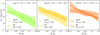 |
Fig. 6. Median metallicity among AGN host galaxies (dashed line) and SF galaxies (continuous line) as a function of the galactic radius. The numbers (NAGN, NSF) of the galaxies in the two samples are reported in the legend for each mass bin. Shaded areas cover the upper and lower errors on the metallicity gradients, computed as the 25th and 75th percentiles of the 12 + log O/H distribution inside each stellar mass bin. As expected from the well-known MZR, the nuclear metallicity of both SF and AGN host galaxies constantly increases together with the host galaxy’s stellar mass, saturating at 12 + log O/H ∼ 9.0 for the SF galaxies and rising to ∼9.1 in the AGN hosts. In addition, the metallicity gradients become flatter with higher stellar mass in the SF galaxies. |
Accordingly to the plateau typically observed in the MZR of SF galaxies (see, e.g., Peluso et al. 2022; Mannucci et al. 2010; Tremonti et al. 2004), the nuclear metallicity of SF galaxies saturates at 12 + log O/Hr < 0.5Re ∼ 9.0, while the nuclear metallicity of the AGN host rises from 12 + log O/Hr < 0.5Re ∼ 9.05 (left and central panels) to 12 + log O/Hr < 0.5Re ∼ 9.1 (right panel), without showing signs of saturation. Also, AGN hosts show higher abundances than SF galaxies at any given radius. We define the following quantity:
which is the ratio of the differences in metallicity between the AGN hosts and SF galaxies in the nuclear regions and in the disk at r ∼ 1.25Re. Therefore, R > 1 means that the metallicity enhancement with respect to SF galaxies in the nuclear regions of AGN hosts is more accentuated than the enhancement observed in the disk. For both 10.5 ≤ log(M*/M⊙)≤10.7 and log(M*/M⊙)≥10.9, R is ∼2.24; at intermediate masses it is 1.77. In other words, the AGN show stronger metal enhancement in their nuclear regions with respect to the one in the disk, regardless of the galaxy’s stellar mass.
In Figure 7, we plot the gradient slopes (Δα) versus the disk’s metallicity, of both AGN hosts (circles) and SF galaxies (stars), regardless of environment and stellar mass. The points are color-coded according to the nuclear metallicity. The black and red lines show the KDE of the SF and AGN host galaxies, respectively. We notice that the slopes are, again, predominantly negative in both the SF and AGN samples.
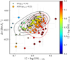 |
Fig. 7. Gradient’s slope (Δα) as a function of the disk metallicity of SF galaxies (stars) and AGN host galaxies (circles) with logM*/M⊙ > 10.5, color-coded according to the nuclear metallicity.Black and red contours represent density curves computed by a KDE. In the legend, we also report the Spearman rank-order correlation coefficient that supports the finding that the SF gradients are strongly correlated with the disk’s metallicity (spSF = 0.54), but the same is not true for the AGN host galaxies. Indeed, AGN hosts have on average steeper slopes than SF due to their higher nuclear metallicities. |
It now appears clear (as already hinted in Figure 6) that the metal enhancement of AGN hosts galaxies is stronger than in SF galaxies in the nuclear regions. At a fixed disk’s metallicity, AGN hosts show steeper slopes than SF galaxies, with the steepness increase linked to their higher nuclear (r < 0.5Re) metallicities. Finally, using a Spearman test we found a significant correlation between the slope Δα and the disk’s metallicity in SF galaxies (spSF = 0.54, with a p-value of 2.3 × 10⁻¹⁰). In contrast, AGN hosts do not show a correlation between the slope and 12 + log O/Hr = 1Re, exhibiting a spAGN of 0.22 (p-value = 1.8 × 10⁻²).
5. Discussion
Thanks to the spatially resolved oxygen abundance maps presented in this work, we were able to observe that AGN host galaxies show higher abundances than SF galaxies at each radius, but that the metal enhancement of the gas in the AGN’s nuclear regions is accentuated with respect to what observed in the HII regions of the galactic disk. In the following, we explain how we checked for the presence or lack of a correlation between the gradients’ slopes and the host’s galaxy properties. Also, we investigate a possible dependence of the results on the method adopted to compute the nuclear abundances, by comparing our results with those presented in Nascimento et al. (2022), using a sample of galaxies in common with this work. We also test the robustness of our metallicity estimates by comparing the oxygen abundances obtained from the SEL calibrators in Sect. 3.2 with those retrieved with calibrators and models from the literature.
5.1. Slopes versus galaxy’s properties
In agreement with an inside-out growth scenario of the spiral discs through the accretion of cold gas streams (Matteucci 1989; Molla et al. 1996; Boissier & Prantzos 1999; Belfiore et al. 2019a), in the previous sections, we explainwe have found that in both AGN and SF galaxies the slopes of the metallicity gradients are mainly negative and range between [0, −0.3] dex  . To investigate the possible causes of the metal enhancement in the AGN-dominated nuclear regions with respect to those of SF galaxies (see Figure 7), we show in Figure 8 the Δαresults forof the AGN (pink circles) and SF (gray stars) galaxies, regardless of their environment, as a function of the [O III] λ5007 luminosity (logL[O III]λ5007r < 1 kpc) and of the host galaxy’s stellar mass, respectively. We consider the L [O III] in the NLR (which, in this case, we approximate to be the region within r < 1 kpc) as a proxy of the AGN’s bolometric luminosity (see, e.g., Berton et al. 2015). The Spearman coefficients reported in the legend of Figure 8 suggest that no correlation exists between these two quantities and the gradient slopes, in both our SF and AGN samples. The main difference between the two samples consists of the fact that SF galaxies reach at most L[O III] ∼ 1041 (erg/s), while AGN host galaxies exceed this threshold. The right panel of Fig. 8 shows that not even a correlation between stellar masses and slopes is in place. We checked that the nuclear luminosity does not scale linearly with the host galaxy’s stellar mass; thus, the SF and AGN relations in the Δα versus logM*/M⊙ are not in contrast with those in the Δα versus log L [O III]λ5007r < 1 kpc diagram. We note that a residual dependence on the spatial resolution of the observation can affect these trends, since in the case of a moderately luminous AGN (such as Seyfert galaxies), the NLR extends from ∼10 pc to ∼1 kpc (Ramos Almeida & Ricci 2017) and, therefore, it is not always resolved in our samples. To confirm the validity of these results, in Appendix A we also re-obtain the very well-studied relation between stellar mass and slopes of the SF gradients, confirming previous studies (e.g., Mingozzi et al. 2020; Belfiore et al. 2017; Franchetto et al. 2020; Khoram & Belfiore 2025). These trends are independent of the method adopted to measure the metallicity. In fact, Mingozzi et al. (2020) and Franchetto et al. (2020) both use MAPPINGS IV (Dopita et al. 2013) models but coupled with the code IZI (Blanc et al. 2014) in the former and with a modified version of PYQZ (Dopita et al. 2013) in the latter; whereas (Belfiore et al. 2017) exploited the calibrations from Pettini & Pagel (2004) and Maiolino et al. (2008), as opposed to this work where we rely on SEL calibrators (Sect. 3.2) based on CLOUDY v17 models coupled with the NEBULABAYES code.
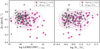 |
Fig. 8. Slopes of the metallicity gradients (Δα) of the AGN (pink points) and SF (gray stars) galaxies as a function of the luminosity of the [O III] λ5007 line within an aperture with r ∼ 1 kpc (logL [O III]λ5007r < 1 kpc) and the host galaxy stellar mass. Pink and gray contours represent density curves computed by a KDE. No clear correlation is observed in both the Δα – L[O III]λ5007 diagram and Δα − logM*/M⊙ diagrams in the SF and AGN samples, as supported by the Spearman rank-order correlation coefficient reported in the legend. |
5.2. Linear fitting of the star-forming disk
To ensure that the results presented in Sect. 4.2 are independent of the method employed to compute the nuclear metallicities in galaxies, we repeated the analysis by applying the approach of Nascimento et al. (2022) (DN22, hereafter). To briefly recap, we not only observed negative gradients in AGNs, indicating that the nuclear (R < 0.5Re) regions of AGNs are more metal enriched than the HII regions in the galactic disk (R > 0.5Re), but also that the enrichment is more enhanced relative to the nuclear regions of a control sample of galaxies without AGN (see Figure 6). This is in contrast with the findings of DN22, who measured lower nuclear metallicities than those extrapolated from a linear fit of observed SF abundances in the galactic disk in a sample of AGN hosts drawn from MaNGA.
DN22 performed a detailed study where they linearly fit the metallicities inside the SF spaxels of a sample of 61 AGN hosts and 112 SF galaxies selected from the DR15 of the MaNGA survey. The metallicity in the SF regions was computed using the Pettini & Pagel (2004) and Pérez-Montero et al. (2019) calibrators. The extrapolated value of the gradient to the galactic center (R = 0) was then compared to the median value of 12 + log O/H inside an aperture with a diameter of 2.5′′ (corresponding to a physical region extending from ∼1 to ∼6 kpc according to the galaxy’s redshift) that was computed by using the Storchi-Bergmann et al. (1998) and Carvalho et al. (2020) calibrators. In DN22, the composite spaxels were discarded.
To apply this kind of analysis to our AGN-FS sample drawn from MaNGA, we fit (as in DN22) the SF regions in our sample of 52 AGN hosts with the relation:
Y = Y0 + grad Y × R,
where Y is a given oxygen abundance – in units of 12 + log O/H – and R is the galactocentric distance (in units of arcsec). Then, Y0 is the extrapolated value of the gradient to the galactic center (R = 0) and grad Y is the slope of the distribution (in units of dex/arcsec). As an example, Figure 9 shows the linear fit of the gradient in the HII regions (yellow/orange line) of the MaNGA galaxy ‘8985-12703’. The red dot marks the median oxygen abundance inside an area equal to the MaNGA PSF (e.g., 12 + log O/HPSF ∼ 2.5′′), which is the smallest resolved region. The linear fit was computed with a non-linear least square method for 42 galaxies out of 52 AGN hosts part of the AGN-FS;, whereas for 10 galaxies, the fit was not able to converge to a solution. Figure 10 displays the difference between 12 + log O/HPSF ∼ 2.5′′ and Y0 extrapolated from the linear fit of the 42 AGN-FS galaxies. The median difference is compatible with zero, as indeed we have ⟨D⟩=0.04 ± 0.15. In contrast, the value found by DN22 is −0.16 (or −0.30 dex, depending on the calibration assumed for the AGN regions). In this work, we find that the metallicity in the AGN-dominated region is slightly higher than expected from pure star formation in galaxies with a stellar masses of logM*/M⊙ ≥ 10.5. The difference becomes significant, ⟨D⟩=0.10 ± 0.09 (noting that only four galaxies have ⟨D⟩≤0) if we consider only the more massive AGN hosts (logM*/M⊙ ≥ 10.9), which show signs of metal pollution induced by the AGN activity,(as observed in the right panel of Figure 6).
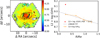 |
Fig. 9. Left: Metallicity map of the AGN-host galaxy ‘8985-12703’ in MaNGA, which is a galaxy in common with the sample studied in Nascimento et al. (2022). The red circle is the MaNGA PSF, e.g., an aperture with diameter d ∼ 2.5′′. Right: Metallicity gradient for the same galaxy. The yellow line traces the median metallicity gradient if only SF spaxels are considered, while the red dot is the median 12 + log O/H inside the MaNGA PSF among all the spaxels (AGN, composite, and SF). Thus, the red dot traces the metallicity in the AGN-dominated region, while the orange gradient shows the metal content of the HII regions in the galaxy’s disk. The black dotted line is the linear fit of the observed HII gradient, obtained with an non-linear least square method. This figure is adapted in order to resemble Figure 3 in Nascimento et al. (2022). |
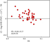 |
Fig. 10. Difference between the median oxygen abundance inside the MaNGA PSF (12 + log O/H PSF ∼ 2.5′′, e.g., red dot in Figure 9) and the oxygen abundance extrapolated at R = 0 (e.g., Y0) from the linear fit, as a function of Y0. The measured metallicity of AGN hosts is systematically higher than the one extrapolated by the linear fit of the HII regions in the galaxy’s center. |
DN22 reported the opposite result, namely,which is that the measured values with the Storchi-Bergmann et al. (1998) and Carvalho et al. (2020) calibrators are systematically lower than the metallicity at R = 0 extracted from the linear fit of the HII regions. In other words, in DN22, the measured nuclear AGN-dominated metallicity is lower than the one expected from a scenario in which star formation is the dominant ionization mechanism at the galaxy’s center. Therefore, the discrepancy seen among the findings in this work and in DN22 could stem from the fact that DN22 used calibrators obtained by different and independent works;, whereas we used calibrators based on consistent assumptions among the AGN, composite, and SF models and using the same code (see Sect. 4).
In addition, it is also important to keep in mind that the classification of AGN and SF regions is based on different criteria;. Meanwhile, we used [N II]-BPT diagram, DN22 relied on the WHAN diagrams proposed by Fernandes et al. (2010), which are based on the Hα equivalent width and log [N II]/Hα. In conclusion, we find that the nuclear regions of a galaxy are more metal-enriched when AGN activity is present, independently of the method adopted to obtain the nuclear metallicity.
5.3. Comparison with AGN- and SF-calibrators from the literature
To further strengthen our analysis and results, in this section, we recomputed the metallicity for all our galaxies using SEL calibrators from the literature and compare the outputs to our estimates obtained with the SF and AGN calibrators given in Eqs. (2) and (3).
To compute the abundances in the SF-classified spaxels, we used the calibrator given in Equation (6) of DN22 and the calibrator taken from Pérez-Montero & Contini (2009) (PC09, hereafter), based on direct Te method estimates. To compute the abundances in the AGN-classified spaxels, we considered the calibrators from Storchi-Bergmann et al. (1998) (SB98, hereafter) and Carvalho et al. (2020) (C20, hereafter), as indeed these equations involve strong emission lines occurring within the MUSE spectral coverage.
Table 1 summarizes the main assumptions made for the calibrators and models retrieved from the literature, in particular: log(N/O) calibration with 12 + log(O/H) in the regime of secondary N production, the shape of the AGN ionizing continuum, the gas density, and solar oxygen abundance. For comparison, we also recap the assumptions made to derive the AGN calibrator presented in this work. The DN22 calibrator is:
Main assumptions behind the calibrators drawn from the literature.
 (6)
(6)
where N2 = log[N II]λ6584/Hα ratio and the P09 calibrator is:
 (7)
(7)
where O3N2 (Alloin et al. 1979) is defined as
![Mathematical equation: $$ \begin{aligned} \mathrm{O3N2} = \log \frac{[{\text{ O}}{\small { {\text{ III}}}}]\lambda 5007}{H\beta } \small {\times } \frac{(\mathrm H\alpha )}{[{\text{ N}}{\small { {\text{ II}}}}]\lambda 6584} .\end{aligned} $$](/articles/aa/full_html/2025/09/aa53370-24/aa53370-24-eq19.gif) (8)
(8)
These relations are valid for 12 + logO/H ≥ 8.0. Figure 11 shows the KDE of the difference between abundances obtained with Equation 2 (e.g., 12 + log O/HP24, SF) and with the P09/DN22 calibrator (top and bottom panels) as a function of 12 + log O/HP24, SF. We color in grey the area spanning a difference between ±0.1 dex, which is the typical uncertainty assumed for the metallicity estimates through SEL calibrators. We find that the standard deviation of the distribution is ≈0.14 dex for both the PC09 and DN22 calibrators, meaning that the difference between our estimates and those from PC09/DN22 is < 0.14 dex for the majority (50%) of the points. As far as the AGN calibrator is concerned, we apply the following SB98 equation:
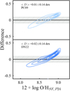 |
Fig. 11. Difference between 12 + log (O/H) inside the SF spaxels of the SF-RPS and SF-FS galaxies computed with the P24 calibrator in Eq. (2) (12 + log O/HSF, P24) and the P09 (top panel) and DN22 (bottom panel) calibrators, as a function of 12 + log O/HSF, P24. The median difference, ⟨D⟩, and the standard deviation (±σ) of the distribution are reported in the legend. |
 (9)
(9)
where x ≡ ([N II]λ6548 + [N II]λ6584)/Hα and y ≡ ([O III]λ4959 + [O III]λ5007)/Hβ. SB98 uses CLOUDY to predict fluxes in case of a segmented power-law radiation field described in Mathews et al. (1987). The model oxygen abundance ranges between 8.4 ≤ 12 + log (O/H) ≤ 9.4 and the ionization parameter −4.0 ≤ log (U) ≤ −2.0. They account for dust depletion and assume secondary-origin nitrogen following Storchi-Bergmann et al. (1994). The gas density is fixed to nH = 300 cm−3. We also adopted the SEL calibrator by C20:
 (10)
(10)
The validity range is −0.7 ≤ N2 ≤ 0.6, which translates to a validity range between 8.16 ≤ 12 + log O/H ≤ 9.0. This relation is obtained by interpolating CLOUDY v17.0 (Ferland et al. 2017) photoionization models to the observed log ([O III]λ5007/[O II]λ3727) versus log ([N II]λ6583/Hα) in a sample of 433 Seyfert from the Sloan Digital Sky Survey DR7 (SDSS DR7, Abazajian et al. 2009) and selected by Dors et al. (2020a).
Figure 12 shows the difference between the abundances in the AGN regions obtained by the different calibrators. In both cases, the difference between abundances from the P24 calibrators and from the C20/SB98 calibrators is < 0.4 dex within 1σ of the distribution. Also, the KDE distributions show that the difference is always higher than zero in both cases. In other words, the SB98 and C20 calibrators tend to underestimate the metallicities with respect to Eq. (3) and the difference linearly increases along with the metallicity.
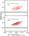 |
Fig. 12. Difference between 12 + log (O/H) inside the AGN spaxels of the AGN-RPS and AGN-FS galaxies computed with the P24 calibrator in Eq. (3) (12 + log O/HAGN, P24) and the C20 (top panel) and SB98 (bottom panel) calibrators, as a function of 12 + log O/HAGN, P24. The median difference, ⟨D⟩, and the standard deviation (±σ) of the distribution are reported in the legend. |
To further investigate this discrepancy, we also compare the abundances obtained with our models and with the MAPPINGSV (Sutherland & Dopita 2017) photo-ionization models presented in Thomas et al. (2018a) (T18 models, hereafter). We applied the T18 models following the same procedure described in Sect. 3, thus comparing the predicted and observed [O III]/[S II]and [N II]/[S II]. The T18 models are plane-parallel, one-dimensional, and dusty, with elemental depletions onto dust grains based on Jenkins (2009). The assumed solar oxygen abundance is 12 + log O H = 8.76. The Seyfert ionizing spectrum is taken from Thomas et al. (2016) and parameterizes the energy of the ionizing accretion disk emission by its peak energy, Epeak, the photon index of the inverse Compton scattered power-law tail, Γ, and the proportion of the total flux that goes into the non-thermal tail, pNT. The only parameter left to vary was Epeak. The other parameters are fixed to the fiducial values Γ = 2.0 and pNT = 0.15. In Figure 13, we show the difference between abundances computed with the T18’s MAPPINGSV models having logEpeak (keV) = −1.25, −1.5, −1.75, −2.0 and 12 + log O/HP24, AGN. We checked that the T18 models do not change significantly as a function of the gas pressure, which we set to log (P/k)=5. We observe a generally good agreement up to logEpeak (keV) = −1.5, with the median difference, ⟨D⟩, equal to 0.04 ± 0.06 dex and 0.09 ± 0.07 dex. The discrepancy starts to increase at logEpeak (keV) = −1.75 with ⟨D⟩=0.13 ± 0.08 dex and becomes significant for logEpeak (keV) = −2.0, having ⟨D⟩=0.23 ± 0.09 dex, which are higher than the 0.1 dex uncertainty associated to the NEBULABAYES parameters estimate (see Figure 2). Thomas et al. (2019) adopted an Epeak = 45 eV, corresponding to log Epeak (keV) ∼ −1.35, as values of Epeak in the range 40–50 eV resulted to be more plausible (Thomas et al. 2018b). In the case of a harder AGN radiation field, we observe that the metallicities decrease and get closer to the values obtained by SB98 and C20. However, as explained in detail in Thomas et al. (2018a), the extreme value of Epeak = 100 eV (e.g., logEpeak = −2.0) is improbably high, considering the ionization potentials of species observed in typical NLRs.
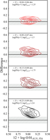 |
Fig. 13. Difference between 12 + log O/HAGN, P24 and the values obtained giving in input to NEBULABAYES the [O III]/[S II]and [N II]/[S II] ratios from MAPPINGSV models (Thomas et al. 2018a) with a peak energy in the AGN accretion disk of logEpeak = −1.25, −1.5, −1.75, and −2.0. The gas pressure is fixed to logP/k = 5, after checking that the results do not change as a function of this parameter. The grey shaded area covers the range ±0.1 dex, which is the uncertainty associated to the parameters estimates with NebulaBayes. The median difference, ⟨D⟩, and the standard deviation (±σ) of the distribution are reported in the legend. |
6. Conclusions
In this work, we explore how the interplay between RPS and AGN activity affects oxygen abundance throughout the galaxy, as well as the influence of AGN activity on the metallicity in the galactic nuclear regions.
To measure the metallicity, we used SEL calibrators (referred to as P24 calibrators) obtained by linearly fitting CLOUDY photoionization models generated assuming ionization from stars, AGN, and a mix of both. With these models, we reproduced the line ratios [N II]/[S II] and [O III]/[S II] to constrain the oxygen abundance and the ionization parameter by matching predictions and observations with the code NEBULABAYES. To validate the use of our new set of SEL calibrators, we compared the P24 calibrators with widely used calibrators retrieved from the literature.
First, we measured the spatially resolved gas-phase metallicity of 10 AGNs experiencing RPS from the GASP survey and 52 undisturbed field AGNs from the MaNGA DR15. We find that:
-
(i)
The metallicity distributions of stripped and non-stripped AGN are statistically indistinguishable within r < 1.5Re, with the only exception of two RPS galaxies, JO206 and JO171, which show lower (see Figure 5) abundances at any given radius than the rest of the AGN-RPS and AGN-FS galaxies.
The above finding shows that the synergy between AGN and RPS does not play a major role in altering the gas-phase metallicity in the GASP galaxies. This result aligns with the fact that the GASP sample consists of stripped galaxies likely experiencing the peak intensity of RPS. This is supported by their enhanced SFR with respect to main sequence galaxies (Vulcani et al. 2018), which is expected during the peak intensity phase of RP (Ricarte et al. 2020). In addition, they feature remarkably long gas tails that extend for tens of kpc along with star-forming knots (Gullieuszik et al. 2023; Giunchi et al. 2023). According to simulations by Ricarte et al. (2020), the combined effect of RPS and AGN feedback on the metallicity distribution becomes significantly effective and induce a decline of the SFR, and consequently of the metal pollution, by a factor of 10 over a few Myrs after the RP peak intensity. Therefore, to better characterize the link between the two phenomena, we would need larger samples of RPS galaxies captured after the RP peak phase. However, we speculate that these observations would be extremely challenging due to the faintness of the gas emission in these low-SFR systems.
By including a control sample of 83 SF galaxies, we further explore the effect of the AGN activity on the metallicity distributions. We compared the metallicity gradients of these galaxies with those of AGN in both clusters and the field, allowing us to analyze the effects independently of the galaxy environments. All galaxies considered have stellar masses of log(M*/M⊙)≥10.5 and are observed at redshift z < 0.07. We find that:
-
(ii)
AGN hosts show higher metallicities than SF galaxies at any radius. However, the AGN hosts present a metal enrichment in the nuclear regions (r < 0.5Re) higher by a factor ranging between 1.8 and 2.3 times the enhancement shown in the disk at r ∼ 1.25Re (see Figure 4), depending on the galaxy’s stellar mass. In particular, this factor is 2.3, 1.77, and 2.24 in the mass bins of 10.5 ≤ logM*/M⊙ ≤ 10.7, 10.7 ≤ logM*/M⊙ ≤ 10.9, and 10.9 ≤ logM*/M⊙ ≤ 11.1.
-
(iii)
In both SF and AGN galaxies, the slopes of the radial profile are not significantly correlated with other galaxy properties, such as the nuclear [O III] luminosity (logL[O III]λ5007r<1 kpc) and host galaxy stellar mass (logM*/M⊙).
The enhanced metallicity observed in AGN can be explained on the basis of several different hypotheses. One explanation is that the gas is enriched in metals from the dissociation and disruption of dust that pollutes the ISM in the SMBH’s vicinity (Maiolino & Mannucci 2019). Another possible explanation for the difference in metallicity distributions between SF galaxies and AGN hosts is the reduced SFR associated with the presence of an AGN, rather than by the AGN itself (Li et al. 2025; Schawinski et al. 2014; Ellison et al. 2016; Lacerda et al. 2020). This reduced SFR could lead to higher metallicity in AGN hosts, as the relationship between SFR and metallicity is known to be anti-correlated according to the fundamental metallicity relation (FMZR, Mannucci et al. 2010). Li et al. (2025) proposed two possible mechanisms to explain the suppressed SFR in AGNs. One is “gentle” AGN negative feedback that prevents gas accretion (Kumari et al. 2021);. The other possibility is that the growth of the bulge simultaneously triggers both AGN activation and the inhibition of star formation.
Overall, the above considerations and results emphasize the need for multi-frequency information about gas and dust across various ionization stages, with resolutions of ≪1 kpc. In fact, we want to stress once again that there may still be a residual and intrinsic dependence of our results on the spatial resolution (∼1 kpc) of these observations. Sub-kpc spatial resolutions are crucial for resolving the NLR and understanding its metal content, as well as for distinguishing between star formation occurring in the vicinity of AGN and within the galactic disk. An in-depth understanding of these properties is essential for linking observed oxygen abundances to the physical mechanisms underlying their formation.
Data availability
The data tables are available at the CDS via https://cdsarc.cds.unistra.fr/viz-bin/cat/J/A+A/701/A29
The photoionization models used to compute the oxygen abundances in the AGN, HII, and Composite regions are available at the Zenodo link: https://doi.org/10.5281/zenodo.15754541. Similarly, the metallicity radial profiles of the sample of 477 galaxies can be found at the Zenodo link https://doi.org/10.5281/zenodo.15727936.
Photoionization models for the AGN, HII and Composite regions are available at the Zenodo link: https://doi.org/10.5281/zenodo.15754541.
To further test the robustness of our results, we ensured that the metallicity gradients and the derived relations presented throughout the paper are perfectly consistent when computing the metallicity by means of the calibrators or the photoionization models coupled with NebulaBayes. We remind the reader that the main assumptions on the models are the stellar age of t* = 4 × 10⁶ yr, the gas density nH = 102 cm−3, and a slope of the AGN continuum α = −2.0.
The online database containing the maps is available at the Zenodo link: https://doi.org/10.5281/zenodo.15727936.
Acknowledgments
Based on observations collected at the European Organization for Astronomical Research in the Southern Hemisphere under ESO program 196.B-0578. This project has been co-funded by the European Research Council (ERC) under the European Union’s Horizon 2020 research and innovation program (grant agreement No. 833824). GP and ID acknowledge funding from the European Union – NextGenerationEU, RRF M4C2 1.1, Project 2022JZJBHM: “AGN-sCAN: zooming-in on the AGN-galaxy connection since the cosmic noon” – CUP C53D23001120006. JF acknowledges financial support from the UNAM- DGAPA-PAPIIT IN110723 grant, México. This work made use of the KUBEVIZ software which is publicly available at https://github.com/matteofox/kubeviz/. The development of the KUBEVIZ code was supported by the Deutsche Forschungsgemeinschaft via Project IDs: WI3871/1-1 and WI3871/1-2. This work makes use of data from SDSS-IV. Funding for SDSS has been provided by the Alfred P. Sloan Foundation and Participating Institutions. Additional funding toward SDSS-IV has been provided by the U.S. Department of Energy Office of Science. SDSS-IV acknowledges support and resources from the Center for High-Performance Computing at the University of Utah. The SDSS website is www.sdss.org. This research made use of Marvin, a core Python package and web framework for MaNGA data, developed by Brian Cherinka, José Sánchez- Gallego, and Brett Andrews (Cherinka et al. 2019). SDSS-IV is managed by the Astrophysical Research Consortium for the Participating Institutions of the SDSS Collaboration including the Brazilian Participation Group, the Carnegie Institution for Science, Carnegie Mellon University, the Chilean Participation Group, the French Participation Group, Harvard-Smithsonian Center for Astrophysics, Instituto de Astrofísica de Canarias, The Johns Hopkins University, Kavli Institute for the Physics and Mathematics of the Universe (IPMU)/University of Tokyo, Lawrence Berkeley National Laboratory, Leibniz Institut für Astrophysik Potsdam (AIP), Max-Planck-Institufür Astronomie (MPIA Heidelberg), Max-Planck-Institut für Astrophysik (MPA Garching), Max-Planck-Institut für Extra- terrestrische Physik (MPE), National Astronomical Observa- tory of China, New Mexico State University, New York University, University of Notre Dame, Observatário Nacional/ MCTI, The Ohio State University, Pennsylvania State University, Shanghai Astronomical Observatory, United King- dom Participation Group, Universidad Nacional Autónoma de México, University of Arizona, University of Colorado Boulder, University of Oxford, University of Portsmouth, University of Utah, University of Virginia, University of Washington, University of Wisconsin, Vanderbilt University, and Yale University. The MaNGA data used in this work are publicly available at http://www.sdss.org/dr15/manga/manga-data/.
References
- Abazajian, K. N., Adelman-McCarthy, J. K., Agüeros, M. A., et al. 2009, ApJS, 182, 543 [Google Scholar]
- Akerman, N., Tonnesen, S., Poggianti, B. M., Smith, R., & Marasco, A. 2023, ApJ, 948, 18 [NASA ADS] [CrossRef] [Google Scholar]
- Aller, L. H. 1987, in Spectroscopy of astrophysical plasmas (A88-37862 15-90) (Cambridge and New York: Cambridge University Press) [Google Scholar]
- Alloin, D., Collin-Souffrin, S., Joly, M., & Vigroux, L. 1979, A&A, 78, 200 [Google Scholar]
- Amiri, A., Knapen, J. H., Comerón, S., Marconi, A., & Lehmer, B. D. 2024, A&A, 689, A193 [NASA ADS] [CrossRef] [EDP Sciences] [Google Scholar]
- Armah, M., Rog, R., Riffel, R., et al. 2023, MNRAS, 520, 1687 [NASA ADS] [CrossRef] [Google Scholar]
- Arribas, S., Colina, L., Bellocchi, E., Maiolino, R., & Villar-Martín, M. 2014, A&A, 568, A14 [NASA ADS] [CrossRef] [EDP Sciences] [Google Scholar]
- Asplund, M., Grevesse, N., Sauval, A. J., & Scott, P. 2009, ARA&A, 47, 481 [NASA ADS] [CrossRef] [Google Scholar]
- Bacchini, C., Mingozzi, M., Poggianti, B. M., et al. 2023, ApJ, 950, 24 [NASA ADS] [CrossRef] [Google Scholar]
- Bacon, R., Accardo, M., Adjali, L., et al. 2010, SPIE, 7735, 773508 [Google Scholar]
- Baldwin, J. A., Phillips, M. M., Terlevich, R., et al. 1981, PASP, 93, 5 [NASA ADS] [CrossRef] [Google Scholar]
- Barnes, J. E., Hernquist, L. E., Barnes, J. E., & Hernquist, L. E. 1991, ApJ, 370, L65 [NASA ADS] [CrossRef] [Google Scholar]
- Barnes, J. E., Hernquist, L., Barnes, J. E., & Hernquist, L. 1996, ApJ, 471, 115 [NASA ADS] [CrossRef] [Google Scholar]
- Belfiore, F., Maiolino, R., Tremonti, C., et al. 2017, MNRAS, 469, 151 [Google Scholar]
- Belfiore, F., Vincenzo, F., Maiolino, R., & Matteucci, F. 2019a, MNRAS, 487, 456 [NASA ADS] [CrossRef] [Google Scholar]
- Belfiore, F., Westfall, K. B., Schaefer, A., et al. 2019b, AJ, 158, 160 [CrossRef] [Google Scholar]
- Bell, E. F., de Jong, R. S., Bell, E. F., & de Jong, R. S. 2001, ApJ, 550, 212 [CrossRef] [Google Scholar]
- Belley, J., Roy, J.-R., Belley, J., & Roy, J.-R. 1992, ApJS, 78, 61 [Google Scholar]
- Berentzen, I., Shlosman, I., Martinez-Valpuesta, I., & Heller, C. 2007, ApJ, 666, 189 [Google Scholar]
- Berton, M., Foschini, L., Ciroi, S., et al. 2015, A&A, 578, A28 [NASA ADS] [CrossRef] [EDP Sciences] [Google Scholar]
- Bischetti, M., Piconcelli, E., Feruglio, C., et al. 2019, A&A, 628, A118 [NASA ADS] [CrossRef] [EDP Sciences] [Google Scholar]
- Blanc, G. A., Kewley, L., Vogt, F. P. A., & Dopita, M. A. 2014, ApJ, 798, 99 [NASA ADS] [CrossRef] [Google Scholar]
- Blanton, M. R., Kazin, E., Muna, D., Weaver, B. A., & Price-Whelan, A. 2011, AJ, 142, 31 [NASA ADS] [CrossRef] [Google Scholar]
- Boissier, S., & Prantzos, N. 1999, MNRAS, 307, 857 [NASA ADS] [CrossRef] [Google Scholar]
- Boselli, A., Fossati, M., & Sun, M. 2022, A&A Rev., 30, 1 [Google Scholar]
- Bundy, K. 2015, IAUS, 311, 100 [Google Scholar]
- Cappellari, M. 2017, MNRAS, 466, 798 [Google Scholar]
- Cardelli, J. A., Clayton, G. C., & Mathis, J. S. 1989, ApJ, 345, 245 [Google Scholar]
- Carvalho, S. P., Dors, O. L., Cardaci, M. V., et al. 2020, MNRAS, 492, 5675 [NASA ADS] [CrossRef] [Google Scholar]
- Chabrier, G. 2003, PASP, 115, 763 [Google Scholar]
- Chen, Q. H., Grasha, K., Battisti, A. J., et al. 2023, MNRAS, 519, 4801 [NASA ADS] [CrossRef] [Google Scholar]
- Cherinka, B., Andrews, B. H., Sánchez-Gallego, J., et al. 2019, AJ, 158, 74 [CrossRef] [Google Scholar]
- Combes, F., Elmegreen, B. G., Combes, F., & Elmegreen, B. G. 1993, A&A, 271, 391 [Google Scholar]
- Consolandi, G., Gavazzi, G., Fossati, M., et al. 2017, A&A, 606, A83 [NASA ADS] [CrossRef] [EDP Sciences] [Google Scholar]
- Davé, R., Oppenheimer, B. D., & Finlator, K. 2011, MNRAS, 415, 11 [Google Scholar]
- Dekel, A., & Mandelker, N. 2014, MNRAS, 444, 2071 [NASA ADS] [CrossRef] [Google Scholar]
- Dekel, A., Zolotov, A., Tweed, D., et al. 2013, MNRAS, 435, 999 [Google Scholar]
- D’Odorico, V., Cristiani, S., Romano, D., Granato, G. L., & Danese, L. 2004, MNRAS, 351, 976 [CrossRef] [Google Scholar]
- Dopita, M. A., Kewley, L. J., Heisler, C. A., & Sutherland, R. S. 2000, ApJ, 542, 224 [NASA ADS] [CrossRef] [Google Scholar]
- Dopita, M. A., Sutherland, R. S., Nicholls, D. C., Kewley, L. J., & Vogt, F. P. A. 2013, ApJS, 208, 10 [NASA ADS] [CrossRef] [Google Scholar]
- Dopita, M. A., Shastri, P., Davies, R., et al. 2015, ApJS, 217, 12 [NASA ADS] [CrossRef] [Google Scholar]
- Dors, O. L. 2021, MNRAS, 507, 466 [NASA ADS] [CrossRef] [Google Scholar]
- Dors, O. L., Cardaci, M. V., & Krabbe, A. C. 2017, MNRAS, 466, 726 [NASA ADS] [CrossRef] [Google Scholar]
- Dors, O. L., Freitas-Lemes, P., Amôres, E. B., et al. 2020a, MNRAS, 492, 468 [NASA ADS] [CrossRef] [Google Scholar]
- Dors, O. L., Maiolino, R., Cardaci, M. V., et al. 2020b, MNRAS, 496, 3209 [NASA ADS] [CrossRef] [Google Scholar]
- Ellison, S. L., Teimoorinia, H., Rosario, D. J., & Mendel, J. T. 2016, MNRAS, 458, L34 [NASA ADS] [CrossRef] [Google Scholar]
- Ferland, G. J., Chatzikos, M., Guzmán, F., et al. 2017, RMxAA, 53, 385 [NASA ADS] [Google Scholar]
- Fernandes, R. C., Stasinska, G., Mateus, A., & Asari, N. V. 2010, MNRAS, 413, 1687 [Google Scholar]
- Feruglio, C., Maiolino, R., Piconcelli, E., et al. 2010, A&A, 518, L155 [NASA ADS] [CrossRef] [EDP Sciences] [Google Scholar]
- Feruglio, C., Ferrara, A., Bischetti, M., et al. 2017, A&A, 608, A30 [NASA ADS] [CrossRef] [EDP Sciences] [Google Scholar]
- Flury, S. R., & Moran, E. C. 2020, MNRAS, 496, 2191 [NASA ADS] [CrossRef] [Google Scholar]
- Fossati, M., Fumagalli, M., Boselli, A., et al. 2016, MNRAS, 455, 2028 [Google Scholar]
- Fotopoulou, S., Buchner, J., Georgantopoulos, I., et al. 2016, A&A, 587, A142 [NASA ADS] [CrossRef] [EDP Sciences] [Google Scholar]
- Franchetto, A., Vulcani, B., Poggianti, B. M., et al. 2020, ApJ, 895, 106 [NASA ADS] [CrossRef] [Google Scholar]
- Franchetto, A., Mingozzi, M., Poggianti, B. M., et al. 2021, ApJ, 923, 28 [NASA ADS] [CrossRef] [Google Scholar]
- Fritz, J., Moretti, A., Gullieuszik, M., et al. 2017, ApJ, 848, 132 [NASA ADS] [CrossRef] [Google Scholar]
- Gavazzi, G., Contursi, A., Carrasco, L., et al. 1995, A&A, 304, 325 [NASA ADS] [Google Scholar]
- Gavazzi, G., Boselli, A., Mayer, L., et al. 2001, ApJ, 563, L23 [Google Scholar]
- Gibson, B. K., Pilkington, K., Brook, C. B., Stinson, G. S., & Bailin, J. 2013, A&A, 554, A47 [CrossRef] [EDP Sciences] [Google Scholar]
- Giunchi, E., Gullieuszik, M., Poggianti, B. M., et al. 2023, ApJ, 949, 72 [NASA ADS] [CrossRef] [Google Scholar]
- Grevesse, N., Sauval, A. J., & van Dishoeck, E. F. 1984, A&A, 141, 10 [NASA ADS] [Google Scholar]
- Grisoni, V., Spitoni, E., & Matteucci, F. 2018, MNRAS, 481, 2570 [NASA ADS] [Google Scholar]
- Groves, B. A., Heckman, T. M., & Kauffmann, G. 2006, MNRAS, 371, 1559 [NASA ADS] [CrossRef] [Google Scholar]
- Gullieuszik, M., Poggianti, B. M., McGee, S. L., et al. 2020, ApJ, 899, 13 [Google Scholar]
- Gullieuszik, M., Giunchi, E., Poggianti, B. M., et al. 2023, ApJ, 945, 54 [NASA ADS] [CrossRef] [Google Scholar]
- Gunn, J. E., Siegmund, W. A., Mannery, E. J., et al. 2006, AJ, 131, 2332 [NASA ADS] [CrossRef] [Google Scholar]
- Haardt, F., Maraschi, L., Haardt, F., & Maraschi, L. 1993, ApJ, 413, 507 [NASA ADS] [CrossRef] [Google Scholar]
- Heckman, T. M., Lehnert, M. D., Strickland, D. K., & Armus, L. 2000, ApJS, 129, 493 [Google Scholar]
- Hughes, T. M., Cortese, L., Boselli, A., Gavazzi, G., & Davies, J. I. 2013, A&A, 550, A115 [NASA ADS] [CrossRef] [EDP Sciences] [Google Scholar]
- Jenkins, E. B. 2009, ApJ, 700, 1299 [Google Scholar]
- Kauffmann, G., Heckman, T. M., Tremonti, C., et al. 2003, MNRAS, 346, 1055 [Google Scholar]
- Kewley, L. J., Rupke, D., Zahid, H. J., Geller, M. J., & Barton, E. J. 2010, ApJ, 721, L48 [NASA ADS] [CrossRef] [Google Scholar]
- Khoram, A. H., & Belfiore, F. 2025, A&A, 693, A150 [NASA ADS] [CrossRef] [EDP Sciences] [Google Scholar]
- Khoram, A., Poggianti, B., Moretti, A., et al. 2024, A&A, 686, A261 [NASA ADS] [CrossRef] [EDP Sciences] [Google Scholar]
- Kumari, N., Maiolino, R., Trussler, J., et al. 2021, A&A, 656, A140 [NASA ADS] [CrossRef] [EDP Sciences] [Google Scholar]
- Lacerda, E. A. D., Sánchez, S. F., Fernandes, R. C., et al. 2020, MNRAS, 492, 3073 [NASA ADS] [CrossRef] [Google Scholar]
- Law, D. R., Cherinka, B., Yan, R., et al. 2016, AJ, 152, 83 [Google Scholar]
- Li, S.-L., Li, Z., Wisnioski, E., et al. 2025, MNRAS, 536, 430 [Google Scholar]
- Maiolino, R., & Mannucci, F. 2019, A&A Rev., 27, 1 [CrossRef] [Google Scholar]
- Maiolino, R., Nagao, T., Grazian, A., et al. 2008, A&A, 488, 463 [NASA ADS] [CrossRef] [EDP Sciences] [Google Scholar]
- Mannucci, F., Cresci, G., Maiolino, R., Marconi, A., & Gnerucci, A. 2010, MNRAS, 408, 2115 [NASA ADS] [CrossRef] [Google Scholar]
- Mathews, W. G., Ferland, G. J., Mathews, W. G., & Ferland, G. J. 1987, ApJ, 323, 456 [NASA ADS] [CrossRef] [Google Scholar]
- Matsuoka, K., Nagao, T., Marconi, A., et al. 2013, IAUS, 290, 273 [Google Scholar]
- Matteucci, F. 1989, MNRAS, 239, 885 [Google Scholar]
- Mingozzi, M., Belfiore, F., Cresci, G., et al. 2020, A&A, 636, A42 [NASA ADS] [CrossRef] [EDP Sciences] [Google Scholar]
- Molla, M., Ferrini, F., Diaz, A. I., et al. 1996, ApJ, 466, 668 [Google Scholar]
- Moretti, A., Poggianti, B. M., Gullieuszik, M., et al. 2018, MNRAS, 475, 4055 [NASA ADS] [Google Scholar]
- Nascimento, J. C. D., Dors, O. L., Storchi-Bergmann, T., et al. 2022, MNRAS, 513, 807 [CrossRef] [Google Scholar]
- Nayakshin, S., & Sunyaev, R. 2005, MNRAS, 364, L23 [CrossRef] [Google Scholar]
- Nicholls, D. C., Sutherland, R. S., Dopita, M. A., Kewley, L. J., & Groves, B. A. 2017, MNRAS, 466, 4403 [Google Scholar]
- O’Donnell, J. E. 1994, ApJ, 422, 158 [Google Scholar]
- Osterbrock, D. E. 2006, Astrophysics of Gaseous Nebulae and Active Galactic Nuclei (Sausalito, CA: University Science Books) [Google Scholar]
- Pace, Z. J., Tremonti, C., Chen, Y., et al. 2019a, ApJ, 883, 1 [NASA ADS] [CrossRef] [Google Scholar]
- Pace, Z. J., Tremonti, C., Chen, Y., et al. 2019b, ApJ, 883, 83 [Google Scholar]
- Peluso, G., Vulcani, B., Poggianti, B. M., et al. 2022, ApJ, 927, 130 [NASA ADS] [CrossRef] [Google Scholar]
- Peluso, G., Radovich, M., Moretti, A., et al. 2023, ApJ, 958, 147 [NASA ADS] [CrossRef] [Google Scholar]
- Pérez-Díaz, B., Masegosa, J., Márquez, I., & Pérez-Montero, E. 2021, MNRAS, 505, 4289 [CrossRef] [Google Scholar]
- Pérez-Montero, E. 2014, MNRAS, 441, 2663 [CrossRef] [Google Scholar]
- Pérez-Montero, E., & Contini, T. 2009, MNRAS, 398, 949 [CrossRef] [Google Scholar]
- Pérez-Montero, E., Dors, O. L., Vílchez, J. M., et al. 2019, MNRAS, 489, 2652 [CrossRef] [Google Scholar]
- Pettini, M., & Pagel, B. E. 2004, MNRAS, 348, L59 [NASA ADS] [CrossRef] [Google Scholar]
- Pilkington, K., Few, C. G., Gibson, B. K., et al. 2012, A&A, 540, A56 [NASA ADS] [CrossRef] [EDP Sciences] [Google Scholar]
- Poetrodjojo, H., Groves, B., Kewley, L. J., et al. 2018, MNRAS, 479, 5235 [Google Scholar]
- Pogge, R. W. 1988, ApJ, 332, 702 [NASA ADS] [CrossRef] [Google Scholar]
- Poggianti, B. M., Moretti, A., Gullieuszik, M., et al. 2017, ApJ, 844, 48 [Google Scholar]
- Poggianti, B. M., Ignesti, A., Gitti, M., et al. 2019, ApJ, 887, 155 [Google Scholar]
- Poggianti, B. M., Vulcani, B., Tomicic, N., et al. 2025, A&A, 699, A357 [NASA ADS] [CrossRef] [EDP Sciences] [Google Scholar]
- Prantzos, N., & Boissier, S. 1999, MNRAS, 313, 338 [Google Scholar]
- Prochaska, J. X., Werk, J. K., Worseck, G., et al. 2017, ApJ, 837, 169 [CrossRef] [Google Scholar]
- Ramos Almeida, C., & Ricci, C. 2017, Nat. Astron., 1, 679 [Google Scholar]
- Ramos-Martínez, M., Gómez, G. C., & Pérez-Villegas, A. 2018, MNRAS, 476, 3781 [CrossRef] [Google Scholar]
- Ricarte, A., Tremmel, M., Natarajan, P., et al. 2020, ApJ, 895, L8 [NASA ADS] [CrossRef] [Google Scholar]
- Roman-Oliveira, F. V., Chies-Santos, A. L., del Pino, B. R., et al. 2018, MNRAS, 484, 892 [Google Scholar]
- Sánchez, H. D., Huertas-Company, M., Bernardi, M., Tuccillo, D., & Fischer, J. L. 2018, MNRAS, 476, 3661 [CrossRef] [Google Scholar]
- Sánchez-García, O., Sodi, B. C., Fritz, J., et al. 2023, ApJ, 945, 99 [CrossRef] [Google Scholar]
- Schawinski, K., Urry, C. M., Simmons, B. D., et al. 2014, MNRAS, 440, 889 [Google Scholar]
- Schlafly, E. F., & Finkbeiner, D. P. 2010, ApJ, 737, 103 [Google Scholar]
- Schlegel, D. J., Finkbeiner, D. P., & Davis, M. F. 1998, ApJ, 500, 525 [NASA ADS] [CrossRef] [Google Scholar]
- Schulz, S., & Struck, C. 2001, MNRAS, 328, 185 [NASA ADS] [CrossRef] [Google Scholar]
- Smee, S. A., Gunn, J. E., Uomoto, A., et al. 2013, AJ, 146, 32 [Google Scholar]
- Storchi-Bergmann, T., & Schnorr-Müller, A. 2019, Nature, 3, 48 [Google Scholar]
- Storchi-Bergmann, T., Calzetti, D., Kinney, A. L., et al. 1994, ApJ, 429, 572 [NASA ADS] [CrossRef] [Google Scholar]
- Storchi-Bergmann, T., Schmitt, H. R., Calzetti, D., & Kinney, A. L. 1998, AJ, 115, 909 [NASA ADS] [CrossRef] [Google Scholar]
- Sun, M., Ge, C., Luo, R., et al. 2021, Nat. Astron., 6, 270 [NASA ADS] [CrossRef] [Google Scholar]
- Sutherland, R. S., & Dopita, M. A. 2017, ApJS, 229, 34 [Google Scholar]
- Swinbank, A. M., Harrison, C. M., Tiley, A. L., et al. 2019, MNRAS, 487, 381 [Google Scholar]
- Tempel, E., Tamm, A., Gramann, M., et al. 2014, VizieR Online Data Catalog: J/A+A/566/A1 [Google Scholar]
- Thomas, A. D., Groves, B. A., Sutherland, R. S., et al. 2016, ApJ, 833, 266 [NASA ADS] [CrossRef] [Google Scholar]
- Thomas, A. D., Dopita, M. A., Kewley, L. J., et al. 2018a, ApJ, 856, 89 [NASA ADS] [CrossRef] [Google Scholar]
- Thomas, A. D., Kewley, L. J., Dopita, M. A., et al. 2018b, ApJ, 861, L2 [NASA ADS] [CrossRef] [Google Scholar]
- Thomas, A. D., Kewley, L. J., Dopita, M. A., et al. 2019, ApJ, 874, 100 [NASA ADS] [CrossRef] [Google Scholar]
- Tissera, P. B., Machado, R. E., Carollo, D., et al. 2018, MNRAS, 473, 1656 [NASA ADS] [CrossRef] [Google Scholar]
- Tomicic, N., Hughes, A., Kreckel, K., et al. 2018, ApJ, 869, L38 [CrossRef] [Google Scholar]
- Tonnesen, S., Bryan, G. L., Tonnesen, S., & Bryan, G. L. 2009, ApJ, 694, 789 [NASA ADS] [CrossRef] [Google Scholar]
- Tremonti, C. A., Heckman, T. M., Kauffmann, G., et al. 2004, ApJ, 613, 898 [Google Scholar]
- Tremonti, C. A., Moustakas, J., Diamond-Stanic, A. M., et al. 2007, ApJ, 663, L77 [NASA ADS] [CrossRef] [Google Scholar]
- Tumlinson, J., Peeples, M. S., & Werk, J. K. 2017, ARA&A, 55, 389 [Google Scholar]
- Unger, S. W., Pedlar, A., Axon, D. J., et al. 1987, MNRAS, 228, 671 [NASA ADS] [CrossRef] [Google Scholar]
- Veilleux, S., & Osterbrock, D. E. 1987, ApJS, 63, 295 [Google Scholar]
- Veilleux, S., Bolatto, A., Tombesi, F., et al. 2017, ApJ, 843, 18 [Google Scholar]
- Vulcani, B., Poggianti, B. M., Gullieuszik, M., et al. 2018, ApJ, 866, L25 [Google Scholar]
- Vulcani, B., Poggianti, B. M., Tonnesen, S., et al. 2020, ApJ, 899, 98 [Google Scholar]
- Westfall, K. B., Cappellari, M., Bershady, M. A., et al. 2019, AJ, 158, 231 [Google Scholar]
- Zinchenko, I. A., Pilyugin, L. S., Grebel, E. K., Sánchez, S. F., & Vílchez, J. M. 2016, MNRAS, 462, 2715 [Google Scholar]
- Zurita, A., Florido, E., Bresolin, F., Pérez, I., & Pérez-Montero, E. 2021a, MNRAS, 500, 2380 [Google Scholar]
- Zurita, A., Florido, E., Bresolin, F., Pérez-Montero, E., & Pérez, I. 2021b, MNRAS, 500, 2359 [Google Scholar]
Appendix A: Properties of the outliers among the stripped and non-stripped AGNs and slope-stellar mass relation in SF galaxies
In this appendix we present some of the fundamental properties of a sample of "peculiar" galaxies, considered as such due to their significant scatter from the main distributions in Figures 4 and 5. However, an in-depth analysis of the link between these properties and the peculiar metallicity distributions characterizing these galaxies is beyond the scope of this work.
First, we focus on JO206 (z = 0.051, logM*/M⊙ = 10.96) and JO171 (z = 0.052, logM*/M⊙ = 10.61), two GASP galaxies whose metallicity is significantly lower than that covered by the rest of the sample (see Fig. 4). We show in Figure A.1 their spatially resolved metallicity map, metallicity gradient, and map of the [O III]luminosity (L [O III]λ5007) and logU. By considering all the spaxels within a galacticentric distance of r ∼ 1 kpc (e.g., delimitated by the orange circles in the bottom panels of Figure A.1), we find that the median values inside this aperture are logL[O III]λ5007r < 1kpc = 41.45 and logUr < 1kpc = -2.56 for the galaxy JO206, and logL[O III]λ5007r < 1kpc = 39.86 and logUr < 1kpc = -2.74 for the galaxy JO171.
In Figure A.2, we plot logL[O III]λ5007r < 1kpc as a function of logUr < 1kpc on the left panel and logL[O III]λ5007r < 1kpc as a function of the host galaxy’s stellar mass for all the AGN-FS (dark-red triangles) and AGN-RPS (light-red circles), highlighting the "peculiar" galaxies. We observe that JO206 and JO171 do not stand out from the rest of the AGN-RPS sample in terms of their nuclear luminosity or strength of ionization radiation. However, as hinted by its peculiar morphology, JO171 is a rare example of a ring galaxy perturbed by RPS (see Moretti et al. 2018). A joint analysis of the stellar populations and the gas and stellar kinematics performed by Moretti et al. (2018) showed that the origin of the ring was presumably due to a gas accretion event that happened in the distant past, which was then followed by a stripping event consequently to the infall into the massive cluster Abell 3667. Other than that, a recent deep (200 ks) Chandra program targeting JO206 has revealed the presence of an unusually high X-ray luminous AGN (see, e.g., Fotopoulou et al. 2016), with LX = 7-9 1049 erg/s in the 0.5-7.0 keV band (Ignesti, private communication). The currently accepted scenario for the production of X-ray photons around SMBH includes the Comptonization of disk photons in a population of hot thermal electrons (Haardt et al. 1993). The torus is responsible for the obscuration of X-rays due to photoelectric absorption. The Chandra spectrum of JO206 reveals a Compton-thin (e.g., log NH(cm−2) ∼ 22) and obscured (e.g., γ∼ 1.4) hot corona, where the absorbed part of the spectrum is in the 0.5 − 5 keV range.
Next, we focus on 4 MaNGA galaxies, which have steeper slopes than the main distribution of the AGN-FS, going up to α∼ 0.3 dex (see Figure 5). These are the AGN hosts ’8993-12705’ (z = 0.029, logM*/M⊙ = 10.96), ’8311-6104’ (z = 0.027, logM*/M⊙ = 10.67), 8456-3701 (z = 0.026, logM*/M⊙= 10.75), and 9027-12704 (z = 0.035, logM*/M⊙ = 10.69). We show their spatially resolved metallicity maps, metallicity gradients, maps of log L[O III]λ5007, and logU in Figure A.1. The metallicity map of 8456-3701 reveals a highly dishomogenous metal distribution; when joined to the irregular galaxy morphology, this could suggest a strongly disturbed gas distribution residual of a past interaction. It is clear from Figure A.2 that 2 out of 4 galaxies display the highest values of logUr < 1kpc among all the AGN-FS galaxies, while ’8311-6104’ is the highest optically luminous AGN of the sample. The galaxy ’8456-3701’ seems to be characterized by standard luminosity and ionization parameter values.
Figure A.3 shows Δα as a function of L[O III] λ5007r < 1kpc (left panel) and the host’s galaxy stellar mass logM*/M⊙ (right panel), of the AGN-FS (dark red triangles) and AGN-RPS (red circles) galaxies. No clear correlations with the stellar mass nor the [O III] luminosity are observed when considering the whole sample, either in the AGN-FS or AGN-RPS sample. Indeed, for the RPS AGN hosts, the Kendall τ test shows no correlation in the Δα versus logL[O III]λ5007r < 1kpc (kτAGN = −0.16, p-value = 0.36) and Δα versus logM*/M⊙ (kτAGN = −0.07, p-value = 0.29) diagrams. Similarly for the AGN-FS, according to a Kendall τ test, the slopes do not correlate with the galaxy’s properties (τAGN =-0.12, p-value=0.17; and kτAGN =0.12, p-value=0.16). However, the four outliers in Figure 5 still show steeper slopes in both diagrams – as opposed to JO206 and JO171, which lie in the area covered by the main KDE distribution of the AGN-RPS sample. In other words, the field AGNs have also slopes steeper than galaxies in the same range of nuclear luminosity and host galaxy’s stellar mass.
As an ultimate check, we test if the presence of a stellar bar is influencing the metallicity distributions in our samples, and in particular can explain the peculiar behavior observed in the 6 outliers discussed in this section. The influence of the stellar bar on the stellar and gas components is well-known (Berentzen et al. 2007; Combes et al. 1993). Previous works showed that the bar appears to flatten the metallicity gradients inside the bar region (Zurita et al. 2021b,a) or drive a steeper metallicity gradient (Chen et al. 2023). To look for systematic differences induced by the bar in our AGN samples, we divide the galaxies part of the AGN-RPS and AGN-FS into barred and unbarred. Among the AGN-RPS galaxies, Bacchini et al. (2023) found hints of a stellar bar in JO206, as also in JO201, JO204, and JW100 by 3D modeling the CO gas kinematics observed by ALMA at a resolution of ∼ 1 kpc. For the remaining galaxies, we use the classification drawn from the Sánchez-García et al. (2023)’s catalog, in which the unbarred galaxies were JO171 and JW39. For the AGN-FS, we use the classification from the ‘MaNGA Morphology Deep Learning DR17’ catalog (Sánchez et al. 2018). The classification of the ’peculiar galaxies’ described in this section is of strongly barred for 8311-6104 and 9027-12704 (Pbar ≥0.98), while 8993-12705 is at odds with a Pbar = 0.48 and 8456-3701 has no bar signature (Pbar ∼ 0.08). In conclusion, we do not report a correlation between the presence of the stellar bar and the peculiar metallicity distributions in these objects.
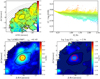 |
Fig. A.1. Top: Metallicity map (on the left) and metallicity gradient (on the right) of the galaxy ’JO206’ (z = 0.051, logM*/M⊙ = 10.96). Bottom: Spatially resolved map of the luminosity of the [O III]λ5007 line (on the left) and ionization parameter log(U) (on the right). The red circle encloses the aperture with a (non-de projected) radius of ∼ 1 kpc, within which the median values of logL[O III] and logU have been computed; this is also noted. These values are also noted on top of the plots (e.g., logL[O III]r < 1kpc and logUr < 1kpc). |
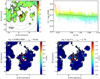 |
Fig. A.1. (continued) Maps and metallicity gradient of the galaxy JO171 (z = 0.052, logM*/M⊙ = 10.61). |
 |
Fig. A.1. (continued) Maps and metallicity gradient of the galaxy 8993-12705 (z = 0.029, logM*/M⊙ = 10.96). |
 |
Fig. A.1. (continued) Maps and metallicity gradient of the galaxy 9027-12704 (z = 0.035, logM*/M⊙ = 10.69). |
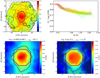 |
Fig. A.1. (continued) Maps and metallicity gradient of the galaxy 8456-3701 (z = 0.026, logM*/M⊙= 10.75). |
 |
Fig. A.1. (continued) Maps and metallicity gradient of the galaxy 8311-6104 (z = 0.027, logM*/M⊙ = 10.67). |
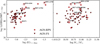 |
Fig. A.2. Median luminosity of the [O III]λ5007 line within r< 1 kpc versus the median value of the ionization parameter inside the same aperture (left panel) and versus the host galaxy’s stellar mass (panel on the right) of the AGN-FS (dark-red trianges) and AGN-RPS (light-red circles). The ’peculiar’ galaxies are highlighted. Overall, the galaxies from the field sample 8311-6104 and 8993-12705 are the most luminous AGNs, with ’8993-12705’ being also the one with the highest ionization parameter followed by 9027-12704. The AGN hosts JO206, JO171, and ’8456-3701’ show standard values of both parameters. |
 |
Fig. A.3. Gradient’s slope (Δα) of the AGN-FS (dark red triangles) and AGN-RPS (red circles) as a function of the [O III] λ5007 luminosity within an aperture of r ∼ 1 kpc (log L [O III]λ5007r < 1kpc) and of the host’s galaxy stellar mass (logM*/M⊙). The legend shows the Kendall τ test’s coefficients (e.g., ktAGN) for the 10 galaxies part of the AGN-RPS and for the 52 galaxies part of the AGN-FS, revealing that the slopes do not correlate with the other galaxy’s properties in both the AGN-RPS and AGN-FS. |
In Figure A.4, we show the gradient slopes of the SF galaxies in both the RPS and field-sample, in the stellar mass range 9.0 ≤logM*/M⊙≤ 11.1. We observe that the slopes are negative at every stellar mass, ranging between [-0.12, -0.24] dexRe−1. In agreement with the findings of Belfiore et al. (2017) and Mingozzi et al. (2020) in the MaNGA survey and with the results from Poetrodjojo et al. (2018) in the SAMI survey, we observe a dependence of the SF metallicity gradients on the stellar mass, with the metallicity gradient nearly flat for low-mass galaxies (M* ∼ 109 M⊙) and progressively steeper (more negative) for more massive galaxies. We also observe a flattening at stellar mass M* ≥ 1010.3 M⊙, similarly to Figure 8 where the cut in mass is M* ≥ 1010.5 M⊙. We attribute the flattening to the saturation of the metallicity at around 12 + log O/H ∼ 9.2 typically observed in HII regions, which can readily be explained by classical inside-out chemical evolution models (Belfiore et al. 2019b).
 |
Fig. A.4. Slopes of the SF gradients as a function of the stellar mass. For a comparison to other works, see the shape of the relation derived by Mingozzi et al. (2020) using the code IZI (Blanc et al. 2014) coupled with MAPPINGS IV photoionization models (e.g., red line in the right panel from Figure 12 of the paper) and by Franchetto et al. (2020) using the PYQZ code (Dopita et al. 2013) coupled with the same models as in Mingozzi et al. (2020). |
All Tables
All Figures
|
Fig. 1. Surfaces of 12 + log O/H versus x ≡ log([N II]/[S II]) and y ≡ log[O III]/[S II], as described by the SF calibrator or Eq. (2) (top panels), COMP calibrator or Eq. (4) (center panels) and AGN calibrator or Eq. (3) (bottom panels), rotated of an angle of 0° (right), 90° (center) and 45° (left). The surfaces are obtained by fitting with a least-squared method the observed [O III]/[S II] and [N II]/[S II] line ratios and the 12 + log O/H computed with NEBULABAYES inside the SF spaxels of all the samples, and the composite and AGN spaxels in the AGN-RPS and AGN-FS. Cells are color-coded according to the value of 12 + log O/H. |
| In the text | |
|
Fig. 2. 12 + log O/H computed by NEBULABAYES (12 + log O/HNeb) versus the difference |
| In the text | |
|
Fig. 3. From top to bottom: Metallicity maps (left panels) and metallicity gradients (right panels) of the cluster-AGN host galaxy (JO49, logM* = 10.68, z = 0.0451), cluster-SF galaxy (JO93, logM* = 10.54, z = 0.037), field-AGN galaxy (‘8311-6104’, logM* = 10.67, z = 0.027), and the field-SF galaxy (‘8329-12701’, logM* = 10.99, z = 0.035), shown from top to bottom. On the left: Black contours are overplotted on the metallicity map to divide the SF, composite, and AGN-like regions, as classified by the [N II]– BPT. The gray dotted ellipses are the annuli that cover the galaxy up to Re ∼ 2.5, proceeding with a step of 0.3 dex, except for the central annulus, which has an inner radius of rin = 0Re and an outer radius of rout = 0.5Re. Inside each annulus, the median value of the 12 + log O/H distribution is computed, along with the 25th and 75th percentiles, considering all the 12 + log O/H values inside the SF, composite, and AGN spaxels. On the right: Metallicity profile (gray line) is, obtained by joining the median values of 12 + log O/H of each annulus, plotted versus the mean value of R/Re inside a given annulus, and t(gray line). The shaded area that covers the range of 12 + log O/H values within the 25th and 75th percentiles. In both panels, the color coding is set according to the value of 12 + log O/H, ranging from 8.0 to 9.4. |
| In the text | |
|
Fig. 4. Diagram comparing each pair of metallicities obtained at different radii for AGN-RPS(red circles) and AGN-FS (dark red triangles). The lines show the probability density distribution evaluated using KDE. The comparison is performed among abundances computed at r < 0.5Re, r = 0.6Re, r = 0.8Re, r = 1.2Re, and r = 1.4Re. |
| In the text | |
|
Fig. 5. Left: Gradient’s slope (Δα) as a function of the nuclear metallicity. The legend shows the Kendall τ test’s coefficients revealing that the slopes seem to correlate with the nuclear metallicity only in the AGN-RPS,(kτAGN = −0.73). Right: Median oxygen abundance of the AGN-RPS galaxies (purple dotted line) and AGN-FS galaxies (blue continuous line), as a function of the galactic radius, spanning a mass range of 10.5 ≤ logM*/M⊙ ≤ 11.5. The shaded areas cover the 25th and 75th percentiles of the abundance distribution inside each annulus. |
| In the text | |
|
Fig. 6. Median metallicity among AGN host galaxies (dashed line) and SF galaxies (continuous line) as a function of the galactic radius. The numbers (NAGN, NSF) of the galaxies in the two samples are reported in the legend for each mass bin. Shaded areas cover the upper and lower errors on the metallicity gradients, computed as the 25th and 75th percentiles of the 12 + log O/H distribution inside each stellar mass bin. As expected from the well-known MZR, the nuclear metallicity of both SF and AGN host galaxies constantly increases together with the host galaxy’s stellar mass, saturating at 12 + log O/H ∼ 9.0 for the SF galaxies and rising to ∼9.1 in the AGN hosts. In addition, the metallicity gradients become flatter with higher stellar mass in the SF galaxies. |
| In the text | |
|
Fig. 7. Gradient’s slope (Δα) as a function of the disk metallicity of SF galaxies (stars) and AGN host galaxies (circles) with logM*/M⊙ > 10.5, color-coded according to the nuclear metallicity.Black and red contours represent density curves computed by a KDE. In the legend, we also report the Spearman rank-order correlation coefficient that supports the finding that the SF gradients are strongly correlated with the disk’s metallicity (spSF = 0.54), but the same is not true for the AGN host galaxies. Indeed, AGN hosts have on average steeper slopes than SF due to their higher nuclear metallicities. |
| In the text | |
|
Fig. 8. Slopes of the metallicity gradients (Δα) of the AGN (pink points) and SF (gray stars) galaxies as a function of the luminosity of the [O III] λ5007 line within an aperture with r ∼ 1 kpc (logL [O III]λ5007r < 1 kpc) and the host galaxy stellar mass. Pink and gray contours represent density curves computed by a KDE. No clear correlation is observed in both the Δα – L[O III]λ5007 diagram and Δα − logM*/M⊙ diagrams in the SF and AGN samples, as supported by the Spearman rank-order correlation coefficient reported in the legend. |
| In the text | |
|
Fig. 9. Left: Metallicity map of the AGN-host galaxy ‘8985-12703’ in MaNGA, which is a galaxy in common with the sample studied in Nascimento et al. (2022). The red circle is the MaNGA PSF, e.g., an aperture with diameter d ∼ 2.5′′. Right: Metallicity gradient for the same galaxy. The yellow line traces the median metallicity gradient if only SF spaxels are considered, while the red dot is the median 12 + log O/H inside the MaNGA PSF among all the spaxels (AGN, composite, and SF). Thus, the red dot traces the metallicity in the AGN-dominated region, while the orange gradient shows the metal content of the HII regions in the galaxy’s disk. The black dotted line is the linear fit of the observed HII gradient, obtained with an non-linear least square method. This figure is adapted in order to resemble Figure 3 in Nascimento et al. (2022). |
| In the text | |
|
Fig. 10. Difference between the median oxygen abundance inside the MaNGA PSF (12 + log O/H PSF ∼ 2.5′′, e.g., red dot in Figure 9) and the oxygen abundance extrapolated at R = 0 (e.g., Y0) from the linear fit, as a function of Y0. The measured metallicity of AGN hosts is systematically higher than the one extrapolated by the linear fit of the HII regions in the galaxy’s center. |
| In the text | |
|
Fig. 11. Difference between 12 + log (O/H) inside the SF spaxels of the SF-RPS and SF-FS galaxies computed with the P24 calibrator in Eq. (2) (12 + log O/HSF, P24) and the P09 (top panel) and DN22 (bottom panel) calibrators, as a function of 12 + log O/HSF, P24. The median difference, ⟨D⟩, and the standard deviation (±σ) of the distribution are reported in the legend. |
| In the text | |
|
Fig. 12. Difference between 12 + log (O/H) inside the AGN spaxels of the AGN-RPS and AGN-FS galaxies computed with the P24 calibrator in Eq. (3) (12 + log O/HAGN, P24) and the C20 (top panel) and SB98 (bottom panel) calibrators, as a function of 12 + log O/HAGN, P24. The median difference, ⟨D⟩, and the standard deviation (±σ) of the distribution are reported in the legend. |
| In the text | |
|
Fig. 13. Difference between 12 + log O/HAGN, P24 and the values obtained giving in input to NEBULABAYES the [O III]/[S II]and [N II]/[S II] ratios from MAPPINGSV models (Thomas et al. 2018a) with a peak energy in the AGN accretion disk of logEpeak = −1.25, −1.5, −1.75, and −2.0. The gas pressure is fixed to logP/k = 5, after checking that the results do not change as a function of this parameter. The grey shaded area covers the range ±0.1 dex, which is the uncertainty associated to the parameters estimates with NebulaBayes. The median difference, ⟨D⟩, and the standard deviation (±σ) of the distribution are reported in the legend. |
| In the text | |
|
Fig. A.1. Top: Metallicity map (on the left) and metallicity gradient (on the right) of the galaxy ’JO206’ (z = 0.051, logM*/M⊙ = 10.96). Bottom: Spatially resolved map of the luminosity of the [O III]λ5007 line (on the left) and ionization parameter log(U) (on the right). The red circle encloses the aperture with a (non-de projected) radius of ∼ 1 kpc, within which the median values of logL[O III] and logU have been computed; this is also noted. These values are also noted on top of the plots (e.g., logL[O III]r < 1kpc and logUr < 1kpc). |
| In the text | |
|
Fig. A.1. (continued) Maps and metallicity gradient of the galaxy JO171 (z = 0.052, logM*/M⊙ = 10.61). |
| In the text | |
|
Fig. A.1. (continued) Maps and metallicity gradient of the galaxy 8993-12705 (z = 0.029, logM*/M⊙ = 10.96). |
| In the text | |
|
Fig. A.1. (continued) Maps and metallicity gradient of the galaxy 9027-12704 (z = 0.035, logM*/M⊙ = 10.69). |
| In the text | |
|
Fig. A.1. (continued) Maps and metallicity gradient of the galaxy 8456-3701 (z = 0.026, logM*/M⊙= 10.75). |
| In the text | |
|
Fig. A.1. (continued) Maps and metallicity gradient of the galaxy 8311-6104 (z = 0.027, logM*/M⊙ = 10.67). |
| In the text | |
|
Fig. A.2. Median luminosity of the [O III]λ5007 line within r< 1 kpc versus the median value of the ionization parameter inside the same aperture (left panel) and versus the host galaxy’s stellar mass (panel on the right) of the AGN-FS (dark-red trianges) and AGN-RPS (light-red circles). The ’peculiar’ galaxies are highlighted. Overall, the galaxies from the field sample 8311-6104 and 8993-12705 are the most luminous AGNs, with ’8993-12705’ being also the one with the highest ionization parameter followed by 9027-12704. The AGN hosts JO206, JO171, and ’8456-3701’ show standard values of both parameters. |
| In the text | |
|
Fig. A.3. Gradient’s slope (Δα) of the AGN-FS (dark red triangles) and AGN-RPS (red circles) as a function of the [O III] λ5007 luminosity within an aperture of r ∼ 1 kpc (log L [O III]λ5007r < 1kpc) and of the host’s galaxy stellar mass (logM*/M⊙). The legend shows the Kendall τ test’s coefficients (e.g., ktAGN) for the 10 galaxies part of the AGN-RPS and for the 52 galaxies part of the AGN-FS, revealing that the slopes do not correlate with the other galaxy’s properties in both the AGN-RPS and AGN-FS. |
| In the text | |
|
Fig. A.4. Slopes of the SF gradients as a function of the stellar mass. For a comparison to other works, see the shape of the relation derived by Mingozzi et al. (2020) using the code IZI (Blanc et al. 2014) coupled with MAPPINGS IV photoionization models (e.g., red line in the right panel from Figure 12 of the paper) and by Franchetto et al. (2020) using the PYQZ code (Dopita et al. 2013) coupled with the same models as in Mingozzi et al. (2020). |
| In the text | |
Current usage metrics show cumulative count of Article Views (full-text article views including HTML views, PDF and ePub downloads, according to the available data) and Abstracts Views on Vision4Press platform.
Data correspond to usage on the plateform after 2015. The current usage metrics is available 48-96 hours after online publication and is updated daily on week days.
Initial download of the metrics may take a while.