| Issue |
A&A
Volume 701, September 2025
|
|
|---|---|---|
| Article Number | A106 | |
| Number of page(s) | 10 | |
| Section | Planets, planetary systems, and small bodies | |
| DOI | https://doi.org/10.1051/0004-6361/202554191 | |
| Published online | 09 September 2025 | |
The Titan wakefield effects due to solar wind streaming
1
Institut für Theoretische Physik IV, Ruhr-Universität Bochum,
44780
Bochum,
Germany
2
Department of Physics, Faculty of Science, Port Said University,
Port Said
42521,
Egypt
3
Centre for Theoretical Physics, The British University in Egypt (BUE), El-Shorouk City,
Cairo,
Egypt
4
Department of Physics, College of Science and Humanities, Al-Kharj, Prince Sattam bin Abdulaziz University,
Al-Kharj
11942,
Saudi Arabia
5
Centre for Mathematical Plasma Astrophysics, Department of Mathematics, KU Leuven,
Celestijnenlaan 200B,
3001
Leuven,
Belgium
★ Corresponding author: This email address is being protected from spambots. You need JavaScript enabled to view it.
Received:
19
February
2025
Accepted:
23
July
2025
Abstract
Motivated by the observations of significant ionospheric escape from Titan by the Cassini spacecraft, and Voyager 1 and 2 observations of the solar wind, we suggest a test-charge approach as an additional mechanism to explain the ion loss caused by the solar wind (SW) interaction with the upper ionosphere of Titan (at altitudes of 1600–1700 km). This approach consists of assuming that a test particle that is inserted into the plasma system and moves with a speed that is higher than the acoustic speed can form a wakefield. This wakefield can drag the ionosphere particles and can thus cause them to escape from the upper ionosphere of Titan. In the upper ionosphere of Titan, most of the plasma species consist of three positive planetary ions (HCNH+, C2H5+, and CH5+) with Maxwellian electrons and streaming SW protons with isothermal electrons. We deduced the electrostatic Debye screening and wakefield potentials caused by a moving test charge, as well as the modified dielectric constant of the ion acoustic waves (IAWs). Using the spacecraft measurements of the plasma configuration at Titan, we carried out a parametric analysis of these fields and found that the normalized Debye potential decreases exponentially with the axial distance. Computational calculations demonstrate, however, that ionosphere particle concentrations and temperatures increase the potential amplitude of the wakefield. Denser and hotter regions provide ionosphere particles with energy and push them to follow the test particle and escape from Titan. Furthermore, the increased density of SW protons amplifies the magnitude of the wakefield potential. The velocity and temperature of the SW protons remain unaffected, however, because their velocity is much higher than the acoustic speed of the plasma system. For ionosphere particles to interact with SW particles, their velocity ranges must therefore be comparable for them to be able to sense and respond to each other. Moreover, we determined the characteristics of the IAWs in the upper ionosphere of Titan for minimum and maximum plasma parameters, where the electric field amplitude of solitary waves ranges from 0.5 to 50 mV/m, the frequency range is 10–500 Hz, and the pulse time duration is 0.01–0.8 s in addition to the test particle. At a distance of z > 100 λD from the test-charge particle, however, the bipolar electric field pulse reaches ≈0.05 mV/m. This agrees well with observed data from the Cassini mission.
Key words: acceleration of particles / Sun: corona / solar wind / Moon
© The Authors 2025
 Open Access article, published by EDP Sciences, under the terms of the Creative Commons Attribution License (https://creativecommons.org/licenses/by/4.0), which permits unrestricted use, distribution, and reproduction in any medium, provided the original work is properly cited.
This article is published in open access under the Subscribe to Open model. This email address is being protected from spambots. You need JavaScript enabled to view it. to support open access publication.
1 Introduction
The solar wind (SW) is a plasma that results from an outflow of energy and mass from the outer solar atmosphere, including the hot solar corona. It primarily consists of protons and electrons, but at low abundance levels, there are α particles and many other ion species. The parameters of the SW are highly variable and depend on many different factors, such as the phase of the solar cycle, the heliocentric distance, or the region of the corona from which the wind emerges. The SW interaction with the planets in the Solar System depends on the physical characteristics of the obstacle, its electromagnetic environments, and its plasma, as well as the solar activity, that is, the SW parameters and the intensity of the solar extreme-ultraviolet (EUV) flux (Goldstein 1998; Gosling 2014; Dubinin et al. 2020). The magnetic fields of magnetized planets such as Earth and Saturn protects their outer atmosphere from the SW, which works as a magnetic umbrella that reflects most of the charged particles from the SW. Conversely, the SW directly interacts with the ionospheres of weakly magnetized planets, such as Mars and Venus, and with unmagnetized moons, such as Titan.
Titan is the largest of the Saturn moons and the only moon in the Solar System with a dense and extended atmosphere that is mainly populated by nitrogen and methane (N2 and CH4) with minor amounts of many nitrile species and hydrocarbons. The neutral molecules in the Titan atmosphere are mainly ionized by the EUV radiation from the Sun and energetic plasma from the magnetosphere of Saturn to form a complex ionosphere at an altitude of about 800 km. The ionosphere represents a link between the neutral atmosphere of Titan and the magnetosphere of Saturn, which plays an important role in the heat and chemical balance of the upper atmosphere. The Voyager flyby made the first observation of the Titan ionosphere (Bird et al. 1997). Since the arrival of Cassini in 2004 and its numerous moon flybys, however, our understanding of the composition of the Titan ionosphere has significantly increased (see Coates et al. 2007; Vuitton et al. 2009; Coates et al. 2012; Ågren et al. 2012; Westlake et al. 2012; Wellbrock et al. 2013; Regoli et al. 2016; Arridge et al. 2016).
One interesting phenomenon on Titan is the ionospheric escape. This is a net loss of ionospheric plasma particles at a rate of ~1024 ions/s. This rate of ion loss is equivalent to 7 tons/Earth day (Coates et al. 2012). In the ion escape process, charged particles such as ions leave the planet or lunar atmosphere or its ionosphere and enter space. The escape processes are generally divided into two main groups: thermal and nonthermal escapes. The thermal escape is also of two types: Jeans escape, and hydrodynamic escape (Strobel 2008; Gronoff et al. 2020). On the other hand, nonthermal escape encompasses a variety of processes, including ion sputtering, which is caused by ions impacting the upper atmosphere of the object; photochemical escape; ionosphere plasma energization; and ion/particle pickup. These various mass-loss processes at Titan were reported and analyzed by Strobel (2008); Tucker & Johnson (2009); Johnson et al. (2010). We introduce a theoretical model to study the ion loss at the Titan ionosphere using an additional mechanism that is called a test-charge approach. This loss may indeed result from the SW interaction with Titan, which energizes the ionosphere ions so that they flow out of its upper ionosphere. Titan spends most of its time in the magnetosphere of Saturn and orbits at 20 Saturn radii (Rs) from the planet. This means that the upper atmosphere of Titan is strongly shielded by the magnetic field of Saturn, which constrains the escape of particles from Titan. Titan lies beyond the umbrella of the magnetosheath of Saturn for a small percentage of about 5% of its orbiting time (Garnier et al. 2009), however, and this time may be sufficient for a substantial escape of charged particles from the ionosphere. Therefore, we propose to use our theoretical model to study the escape process during this period.
An important component are the plasma waves, whose implications and basic characteristics in the Titan atmosphere and its ionosphere were described by a series of works (El-Labany et al. 2012; Salem et al. 2017; Moslem et al. 2019; Ahmed et al. 2020; Yahia et al. 2021). El-Labany et al. (2012) studied the basic properties of the nonlinear ion-acoustic rogue wave in the Titan atmosphere. Their model consisted of a three-component plasma of positive ions, negative ions, and isothermal electrons. Their results showed that modulated ion-acoustic wave packets appear as ion-acoustic rogue waves, while the mass of negative ions causes the energy and the amplitude of the rogue waves to decrease. Salem et al. (2017) used the approach of a self-similar plasma expansion to study compositional losses in the Titan atmosphere. To describe the plasma expansion, they used the self-similar transformation to their proposed set of hydrodynamic basic equations. The results showed the effect of different plasma parameters, that is, density and temperature ratios, on the numerical solutions of the density, velocity, and potential profiles. Moreover, Moslem et al. (2019) studied the escape of protons from the SW, which causes ions to escape from the upper ionosphere of Titan. Their findings showed that when the number density of SW protons is increased, the ion escape is reduced, whereas the effect of electrons is the opposite, it enhances the ion escape. Moreover, the expansion domain does not change for more energetic protons, but a higher temperature ratio of the ionosphere particles and electrons leads to increases in the depletion rate of the density. The ions move faster, which increases the ion loss. Furthermore, the study of the propagation of solitary, shock-like, explosive, and periodic ion-acoustic waves at the Titan ionosphere was discussed by Ahmed et al. (2020). Yahia et al. (2021) discussed the physical properties of the proliferation of super rogue waves in the Titan ionosphere. They proposed that super rogue waves are a good tool for catalyzing the photochemical reaction in the Titan ionosphere. El-Shafeay et al. (2023) investigated the effect of the SW on the ion escape from the upper ionosphere of Venus by the wakefield potential approach. The model indicates the interaction of SW protons with venutian hydrogen and oxygen ions using a test-charge approach to produce ion acceleration and escape. The wakefield potential amplitude increases with altitude and is affected by the plasma density; it decreases with increasing planetary oxygen and SW proton densities, but grows with the SW electron density. The wakefield potential is not much changed by SW proton velocity and temperature. The results offer a plausible explanation for ion loss from the venutian atmosphere and match observations from Venus Express.
We study the effect of the SW in the upper Titan ionosphere (at altitudes 1600–1700 km) and its effect on the ion-loss process. We relied on the observed data obtained by the Cassini spacecraft, as well as Voyager 1 and 2 (Whang et al. 2003; Richardson & Smith 2003; Richardson et al. 2004; Garnier et al. 2009), to build our model. The ion loss in the Titan ionosphere has been studied from a theoretical point of view (Salem et al. 2017; Moslem et al. 2019), also using the self-similar approach applied to a fluid-like model to describe the dynamics of the large amplitude scale of the ionized particles. The proposed method has a number of shortcomings, however, such as the lack of information regarding the characteristic time and length (no scaling parameters), and it can therefore not describe the time evolution of the expansion. We employed another method to avoid these shortcomings. It is called the test-charge approach. This approach enables us to investigate the small amplitude scale of the ion escape in the Titan ionosphere, from which the wakefield potential for IAWs is derived. The basic idea is that when the test particle moves in the plasma system, it can generate an attractive wakefield potential behind it to attract similar charges of ions. This process is similar to what was found in superconductors, which is known as Cooper electron pairing. If the attraction between the electrons is strong enough, it can cancel out the Coulomb interaction that pushes them apart (El-Shafeay et al. 2023). This describes an attraction between the charged particles when the velocity of the moving particles exceeds the acoustic speed (the background medium is at rest in the plasma system). On the other hand, the test-charge approach is effective when the particle speed is quite close to the acoustic speed. In multispecies plasma, the collective effect can thus contribute to the attraction between the charged particles. A similar scenario was proposed by Nambu & Akama (1985) in an electron-ion plasma.
A wakefield arises in a plasma when a charged particle moves with a velocity that is higher than the acoustic speed. This is fairly similar to the wave that is generated in the sea behind a boat. The wakefield produced behind the moving particle forms a region with a defined electric potential. Under normal circumstances, particles with charges of the same sign repel each other. The wakefield modulates the electric field so as to momentarily attract more particles with the same charge, however, and temporarily overcomes the natural repulsion. The wakefield essentially creates an area with an opposing electric field that can draw like-charged particles closer to the moving particle. The wakefield can indeed trap particles. Like a potential well, the wakefield confines surrounding particles. These particles are momentarily trapped and follow the path of the test-charge particle if they lack the energy required to depart the potential created by wakefield, regardless of whether this includes positive or negative particles. The essential condition is that the test-charge particle must exceed the acoustic speed for the wakefield to be created; this condition also holds for positively and negatively charged particles. The charge in the electric wakefield is not relevant; the basic process of attraction in the wakefield remains the same.
The layout of this paper is as follows: Section (2) presents our plasma system, which comprises a four-fluid system of equations and the derivation of a modified dielectric constant for the IAWs, Debye shielding, and wakefield potentials. Section (3) displays the numerical analysis of the wakefield potential caused by a test charge in the upper ionosphere of Titan. Finally, Section (4) summarizes our results and conclusions.
2 The fluid models, and the derivation of the potentials
We wish to provide a parametric analysis of the potential around a moving test charge driven by the SW interaction with the upper ionosphere of Titan at altitudes from 1600 to 1700 km. In this region, three main types of positive ionosphere ions are presented, namely HCNH+, ![Mathematical equation: $\[\mathrm{C}_{2} \mathrm{H}_{5}^{+}\]$](/articles/aa/full_html/2025/09/aa54191-25/aa54191-25-eq3.png) , and
, and ![Mathematical equation: $\[\mathrm{CH}_{5}^{+}\]$](/articles/aa/full_html/2025/09/aa54191-25/aa54191-25-eq4.png) (we refer to them with subscripts 1, 2, and 3, respectively) and Maxwellian electrons (subscript e). They interact with streaming SW protons (sp) and Maxwellian SW electrons (se). Then, the fluid model of this plasma system can be described by the following basic equations (Moslem et al. 2019):
(we refer to them with subscripts 1, 2, and 3, respectively) and Maxwellian electrons (subscript e). They interact with streaming SW protons (sp) and Maxwellian SW electrons (se). Then, the fluid model of this plasma system can be described by the following basic equations (Moslem et al. 2019):
![Mathematical equation: $\[\frac{\partial n_1}{\partial t}+\nabla.\left(n_1 \mathbf{u}_1\right)=0,\]$](/articles/aa/full_html/2025/09/aa54191-25/aa54191-25-eq5.png) (1)
(1)
![Mathematical equation: $\[\left(\frac{\partial}{\partial t}+\mathbf{u}_1. \nabla\right) \mathbf{u}_1+\frac{5}{3} \frac{n_1^{-1 / 3} k_B T_1}{m_1 n_{10}^{2 / 3}} \nabla n_1+\frac{e}{m_1} \nabla \phi=0,\]$](/articles/aa/full_html/2025/09/aa54191-25/aa54191-25-eq6.png) (2)
(2)
![Mathematical equation: $\[\frac{\partial n_2}{\partial t}+\nabla.\left(n_2 \mathbf{u}_2\right)=0,\]$](/articles/aa/full_html/2025/09/aa54191-25/aa54191-25-eq7.png) (3)
(3)
![Mathematical equation: $\[\left(\frac{\partial}{\partial t}+\mathbf{u}_2. \nabla\right) \mathbf{u}_2+\frac{5}{3} \frac{n_2^{-1 / 3} k_B T_2}{m_2 n_{20}^{2 / 3}} \nabla n_2+\frac{e}{m_2} \nabla \phi=0,\]$](/articles/aa/full_html/2025/09/aa54191-25/aa54191-25-eq8.png) (4)
(4)
![Mathematical equation: $\[\frac{\partial n_3}{\partial t}+\nabla.\left(n_3 \mathbf{u}_3\right)=0,\]$](/articles/aa/full_html/2025/09/aa54191-25/aa54191-25-eq9.png) (5)
(5)
![Mathematical equation: $\[\left(\frac{\partial}{\partial t}+\mathbf{u}_3. \nabla\right) \mathbf{u}_3+\frac{5}{3} \frac{n_3^{-1 / 3} k_B T_3}{m_3 n_{30}^{2 / 3}} \nabla n_3+\frac{e}{m_3} \nabla \phi=0,\]$](/articles/aa/full_html/2025/09/aa54191-25/aa54191-25-eq10.png) (6)
(6)
and the streaming SW protons (sp) equations are given by
![Mathematical equation: $\[\frac{\partial n_{s p}}{\partial t}+\nabla.\left(n_{s p} \mathbf{u}_{s p}\right)=0,\]$](/articles/aa/full_html/2025/09/aa54191-25/aa54191-25-eq11.png) (7)
(7)
![Mathematical equation: $\[\left(\frac{\partial}{\partial t}+\mathbf{u}_{s p}. \nabla\right) \mathbf{u}_{s p}+\frac{5}{3} \frac{n_{s p}^{-1 / 3} k_B T_{s p}}{m_{s p} n_{s p 0}^{2 / 3}} \nabla n_{s p}+\frac{e}{m_{s p}} \nabla \phi=0.\]$](/articles/aa/full_html/2025/09/aa54191-25/aa54191-25-eq12.png) (8)
(8)
The third term in the momentum Equations (2), (4), (6), and (8) represents the pressure gradient force, and the fourth term is the electric force E = −∇ϕ, where ϕ is the electrostatic potential. Here, n1, n2, and n3, and u1, u2, and u3 are the number densities and fluid velocities of the ionosphere particles, and nsp, and usp are the number density and the velocity of the streaming SW protons. The background temperatures of the ionosphere particles and the SW protons are T1, T2, T3, and Tsp. m1, m2, m3, and msp, are masses, and kB is the Boltzmann constant.
The number densities of the (inertialess) ionosphere electrons (ne) and SW electrons (nse) in the upper Titan ionosphere are assumed to be Maxwellian and written as
![Mathematical equation: $\[n_e=n_{e 0} ~\exp \left(e \phi / k_B T_e\right),\]$](/articles/aa/full_html/2025/09/aa54191-25/aa54191-25-eq13.png) (9)
(9)
and
![Mathematical equation: $\[n_{s e}=n_{s e 0} ~\exp \left(e \phi / k_B T_{s e}\right).\]$](/articles/aa/full_html/2025/09/aa54191-25/aa54191-25-eq14.png) (10)
(10)
The IAWs can exist under the condition vthi ≪ vph ≪ vthe (where vthi, vph (= ω/k), and vthe are the thermal velocity of the ions, the phase velocity of the propagated wave, and the thermal velocity of the electrons, respectively). This condition justifies our assumption of the isothermality of the electrons and adiabaticity of the ions. In other words, the electrons interact and propagate over many wavelengths λ during one wave period, that is, ω−1vthe ≫ λ. This allows the electrons to remain isothermal because they have sufficient time to equilibrate their temperature throughout the system. Consequently, the temperature fluctuations of the electrons can be neglected. If ion conduction is effectively negligible at ion-acoustic scales, then the pressure can be modeled using a barotropic closure of the form p = Cnγ, where γ = (N + 2)/N is the adiabatic index determined by the number of degrees of freedom N. For ions with three translational degrees of freedom (N = 3), this yields γ = 5/3. The constant C is spatially uniform and reflects the thermodynamic state of the plasma.
Finally, the fluid systems of Equations (1)–(8) are closed by the Poisson equation, which comprises the plasma charge densities of the ionosphere and SW particles and the test particle density of a single test charge qt, as
![Mathematical equation: $\[\begin{aligned}\nabla^2 \phi & =-4 \pi\left[\rho_{plasma}+\rho_{test}\right] \\& =4 \pi e\left(n_e+n_{s e}-n_1-n_2-n_3-n_{s p}\right)-4 \pi q_t \delta\left(\mathbf{r}-\mathbf{v}_t t\right).\end{aligned}\]$](/articles/aa/full_html/2025/09/aa54191-25/aa54191-25-eq15.png) (11)
(11)
Here, ρplasma represents the charge densities of the ionosphere particles, 1, 2, 3, e species, and SW particles, sp, se. On the other hand, ρtest is the test-charge density, qt, which propagates in the ionosphere plasma of Titan. This test-charge particle moves with a constant velocity vt along the z-axis. δ(r − vtt) is a three-dimensional (3D) Dirac delta function with an observation point r.
In the case of the equilibrium state, the neutrality condition is
![Mathematical equation: $\[n_{e 0}+n_{s e 0}=n_{10}+n_{20}+n_{30}+n_{s p 0}.\]$](/articles/aa/full_html/2025/09/aa54191-25/aa54191-25-eq16.png) (12)
(12)
When the space-time Fourier transformation is applied to Eqs. (1)–(8), then the Fourier-transformed number densities in ω-k space (ω is the wave frequency and k is the wavenumber) are
![Mathematical equation: $\[\begin{aligned}n_{11} & =\frac{e}{m_1} \frac{k^2 n_{10}}{R_1} \phi, & n_{21} & =\frac{e}{m_2} \frac{k^2 n_{20}}{R_2} \phi, \\n_{31} & =\frac{e}{m_3} \frac{k^2 n_{30}}{R_3} \phi, & n_{s p 1} & =\frac{e}{m_{s p}} \frac{k^2 n_{s p 0}}{R_{s p}} \phi, \\n_{s e 1} & =\frac{e n_{s e 0}}{k_B T_{s e}} \phi, & n_{e 1} & =\frac{e n_{e 0}}{k_B T_e} \phi,\end{aligned}\]$](/articles/aa/full_html/2025/09/aa54191-25/aa54191-25-eq17.png) (13)
(13)
where
![Mathematical equation: $\[\begin{array}{ll}R_1=\omega^2-\frac{5}{3} k^2 v_1^2, & R_2=\omega^2-\frac{5}{3} k^2 v_2^2 \\R_3=\omega^2-\frac{5}{3} k^2 v_3^2, & R_{s p}=\left(\omega-k u_{s p 0}\right)^2-\frac{5}{3} k^2 v_{s p}^2.\end{array}\]$](/articles/aa/full_html/2025/09/aa54191-25/aa54191-25-eq18.png)
Here, ![Mathematical equation: $\[v_{1}=\left(k_{B} T_{1} / m_{1}\right)^{\frac{1}{2}}, v_{2}=\left(k_{B} T_{2} / m_{2}\right)^{\frac{1}{2}}\]$](/articles/aa/full_html/2025/09/aa54191-25/aa54191-25-eq19.png) and
and ![Mathematical equation: $\[v_{3}=\left(k_{B} T_{3} / m_{3}\right)^{\frac{1}{2}}\]$](/articles/aa/full_html/2025/09/aa54191-25/aa54191-25-eq20.png) are the thermal velocities of positive Titan ions, 1,2 and 3, respectively.
are the thermal velocities of positive Titan ions, 1,2 and 3, respectively. ![Mathematical equation: $\[v_{s p}=\left(k_{B} T_{s p} / m_{s p}\right)^{\frac{1}{2}}\]$](/articles/aa/full_html/2025/09/aa54191-25/aa54191-25-eq21.png) and usp0 indicate the thermal and initial velocities of the streaming SW protons. The observed data show that the SW velocity usp0 is very high compared with the acoustic speed of the system. The SW velocity usp0 ranges in the interval (300–600) × 105 cm/s, whereas the ionosphere plasma acoustic speed of the system ranges in the interval (0.1–1) × 105 cm/s. We therefore used the approximation ω < kusp0 in Eq. (13), and using it in Eq. (11), we obtain
and usp0 indicate the thermal and initial velocities of the streaming SW protons. The observed data show that the SW velocity usp0 is very high compared with the acoustic speed of the system. The SW velocity usp0 ranges in the interval (300–600) × 105 cm/s, whereas the ionosphere plasma acoustic speed of the system ranges in the interval (0.1–1) × 105 cm/s. We therefore used the approximation ω < kusp0 in Eq. (13), and using it in Eq. (11), we obtain
![Mathematical equation: $\[\phi_1(\mathbf{k}, ~\omega)=\frac{8 \pi^2 q_t \delta\left(\omega-\mathbf{k.} \mathbf{v}_t\right)}{k^2 \varepsilon(k, ~\omega)},\]$](/articles/aa/full_html/2025/09/aa54191-25/aa54191-25-eq22.png) (14)
(14)
where ε(k, ω) is the dielectric constant of the IAWs, which can be written as
![Mathematical equation: $\[\varepsilon(k, \omega)=\left[\frac{k^2 \lambda_D^2+1}{k^2 \lambda_D^2}\right]\left[1-\frac{k^2 \lambda_D^2}{k^2 \lambda_D^2+1}\left(\frac{\omega_{p 1}^2}{R_1}+\frac{\omega_{p 2}^2}{R_2}+\frac{\omega_{p 3}^2}{R_3}+\frac{\omega_{p s}^2}{\bar{R}_{s p}}\right)\right].\]$](/articles/aa/full_html/2025/09/aa54191-25/aa54191-25-eq23.png) (15)
(15)
Here, ![Mathematical equation: $\[\bar{R}_{s p}=\left(k u_{s p 0}\right)^{2}-\frac{5}{3} k^{2} v_{s p}^{2}. \lambda_{D}=\left[\left(\lambda_{D_{e}}^{2}+\lambda_{D_{s e}}^{2}\right) / \lambda_{D_{e}}^{2} \lambda_{D_{s e}}^{2}\right]^{-1 / 2}\]$](/articles/aa/full_html/2025/09/aa54191-25/aa54191-25-eq24.png) is the effective Debye length with planetary and SW electron Debye lengths, λDe = (4πe2ne0/kBTe)−1/2, λDse = (4πe2nse0/kBTse)−1/2. Whereas, ωp1 = (4πe2n10/m1)1/2, ωp2 = (4πe2n20/m2)1/2, ωp3 = (4πe2n30/m3)1/2, and ωps = (4πe2nsp0/msp)1/2 are the planetary ion plasma frequencies and the streaming SW proton frequency, respectively. The first term in Eq. (15) represents the independent velocity part, which contributes to the Debye shielding potential. On the other hand, the second term, according to the velocity-dependent part, contributes to the wakefield potential.
is the effective Debye length with planetary and SW electron Debye lengths, λDe = (4πe2ne0/kBTe)−1/2, λDse = (4πe2nse0/kBTse)−1/2. Whereas, ωp1 = (4πe2n10/m1)1/2, ωp2 = (4πe2n20/m2)1/2, ωp3 = (4πe2n30/m3)1/2, and ωps = (4πe2nsp0/msp)1/2 are the planetary ion plasma frequencies and the streaming SW proton frequency, respectively. The first term in Eq. (15) represents the independent velocity part, which contributes to the Debye shielding potential. On the other hand, the second term, according to the velocity-dependent part, contributes to the wakefield potential.
When we take the inverse of the space-time Fourier transformation for Eq. (14) and integrate it with respect to ω, the electrostatic potential at an arbitrary position r and time t becomes (see the appendix)
![Mathematical equation: $\[\phi_1(\mathbf{r}, ~t)=\frac{q_t}{2 \pi^2} \int \frac{exp \left[i \mathbf{k}.\left(\mathbf{r}-\mathbf{v}_t t\right)\right]}{k^2 \varepsilon(\mathbf{k}, ~\omega)} d^3 k.\]$](/articles/aa/full_html/2025/09/aa54191-25/aa54191-25-eq25.png) (16)
(16)
Using Eq. (15) in Eq. (16) and with straightforward algebraic manipulations, the Debye-Hückel and the wakefield potentials were derived (see the appendix),
![Mathematical equation: $\[\phi_D=\frac{q_t}{r} exp \left[\frac{-r}{\lambda_D}\right],\]$](/articles/aa/full_html/2025/09/aa54191-25/aa54191-25-eq26.png) (17)
(17)
and
![Mathematical equation: $\[\begin{aligned}\phi_w(z, t)= & \frac{2 q_t}{z}\left\{1+\left[\frac{\omega_{p 1}^2}{\left(v_t^2-\frac{5}{3} v_1^2\right)}+\frac{\omega_{p 2}^2}{\left(v_t^2-\frac{5}{3} v_2^2\right)}+\frac{\omega_{p 3}^2}{\left(v_t^3-\frac{5}{3} v_3^2\right)}+\frac{\omega_{p s}^2}{\left(u_{s p 0}^2-\frac{5}{3} v_{s p}^2\right)}\right] \lambda_D^2\right\} \\& \times\left\{1-\left[\frac{\omega_{p 1}^2}{\left(v_t^2-\frac{5}{3} v_1^2\right)}+\frac{\omega_{p 2}^2}{\left(v_t^2-\frac{5}{3} v_2^2\right)}+\frac{\omega_{p 3}^2}{\left(v_t^3-\frac{5}{3} v_3^2\right)}+\frac{\omega_{p s}^2}{\left(u_{s p 0}^2-\frac{5}{3} v_{s p}^2\right)}\right] \lambda_D^2\right\}^{-1} \\& \times \cos \left\{\left[\frac{\omega_{p 1}^2}{\left(v_t^2-\frac{5}{3} v_1^2\right)}+\frac{\omega_{p 2}^2}{\left(v_t^2-\frac{5}{3} v_2^2\right)}+\frac{\omega_{p 3}^2}{\left(v_t^3-\frac{5}{3} v_3^2\right)}+\frac{\omega_{p s}^2}{\left(u_{s p 0}^2-\frac{5}{3} v_{s p}^2\right)}\right]^{1 / 2} z\right\}.\end{aligned}\]$](/articles/aa/full_html/2025/09/aa54191-25/aa54191-25-eq27.png) (18)
(18)
3 Parametric study and discussion
We study the effect of the SW particle interaction with the upper ionosphere of Titan on the escape of the ionosphere particles. We propose an additional mechanism called the test-charge approach to study the escape process. To understand the test-charge technique, we can imagine that the test particle is externally inserted into the plasma with a constant speed, while its charge is coupled with the plasma charge density by the space-charge effects. This causes the test charge to be surrounded by a cloud of oppositely charged particles, resulting in the short-range Debye-Hückel potential around the test charge. If the test particle has a positive charge, it is shielded by negative particles, which can create an attractive field for other positive charges. To imagine this, we show in Fig. 1 the interaction of the SW with the Titan ionosphere and also the escape process through the wakefield potential. The inset represents the attractive wakefield potential that formed behind the test particles and which attracts the positive ionosphere particles. This formation involves the attraction between similarly charged particles through the attractive wakefield potential. The influence of this potential on another positive charge decreases as the distance increases. The ionosphere particles accelerated by the energetic streaming SW will overcome the escape velocity of Titan and are able to follow the moving test particle to escape from Titan.
The physical mechanism is that SW particles transfer energy to the system and accelerate ionosphere particles that are dragged by the moving test particle through the wakefield potential. This dragging by the test particle occurs when it moves with a velocity close to the acoustic speed of the ionosphere particles. An additional escape process can exist at Titan when the moving particles overcome the escape velocity of Titan. Therefore, we first determined the escape velocity at Titan and compared it with the acoustic speed of the plasma model. The escape velocity was obtained from the general law of total energy, which is the sum of kinetic energy and gravitational potential energy: ![Mathematical equation: $\[E=\frac{1}{2} m v^{2}-G M m / d\]$](/articles/aa/full_html/2025/09/aa54191-25/aa54191-25-eq28.png) . The escape velocity is Vesc = [2GM/d]1/2, where G is the universal gravitational constant, M is the mass of the central body, and d is the distance between the central body and the escape body (at the point of escape) (Breithaupt 2000). In the case of Titan, with M = 1.35 × 10²³ kg, we studied the escaping particles in the upper ionosphere at altitudes of approximately (1600–1700) km. Consequently, d ~ (18.5–19.5) × 106 m and M = 1.35 × 10²³ kg. Using the previous parameters, we found that the escape velocity at the surface of Titan is approximately Vesc ~ 2.6 × 105 cm/s, whereas at higher altitudes (1600–1700 km), the average value is Vesc ~ 2.1 × 105 cm/s. The average value of the acoustic speed of the plasma system considered (Cs = ωp3 λD) is ~2.3 × 105 cm/s, however. This means that at higher altitudes, the kinetic energy or velocity of ionosphere particles can exceed the escape velocity of Titan, allowing these particles to overcome planetary gravity and escape into space. Other mechanisms might influence the escape process, such as ion heating via Poynting flux dissipation, electron heating through soft electron precipitation, and ion heating associated with broadband extremely low-frequency (BBELF) waves (Strangeway et al. 2005; Shen et al. 2018).
. The escape velocity is Vesc = [2GM/d]1/2, where G is the universal gravitational constant, M is the mass of the central body, and d is the distance between the central body and the escape body (at the point of escape) (Breithaupt 2000). In the case of Titan, with M = 1.35 × 10²³ kg, we studied the escaping particles in the upper ionosphere at altitudes of approximately (1600–1700) km. Consequently, d ~ (18.5–19.5) × 106 m and M = 1.35 × 10²³ kg. Using the previous parameters, we found that the escape velocity at the surface of Titan is approximately Vesc ~ 2.6 × 105 cm/s, whereas at higher altitudes (1600–1700 km), the average value is Vesc ~ 2.1 × 105 cm/s. The average value of the acoustic speed of the plasma system considered (Cs = ωp3 λD) is ~2.3 × 105 cm/s, however. This means that at higher altitudes, the kinetic energy or velocity of ionosphere particles can exceed the escape velocity of Titan, allowing these particles to overcome planetary gravity and escape into space. Other mechanisms might influence the escape process, such as ion heating via Poynting flux dissipation, electron heating through soft electron precipitation, and ion heating associated with broadband extremely low-frequency (BBELF) waves (Strangeway et al. 2005; Shen et al. 2018).
To study the escape process in the upper ionosphere of Titan, we proposed the test-charge approach. In this approach, a moving test particle forms a wakefield potential behind it, and this potential pulls/drags similar particles out of Titan. The attraction between particles with the same charge occurs when the velocity of the moving charged particles exceeds the acoustic speed. In other words, this requires an attractive wake potential, which can exist when the wakefield potential is negative (attractive). The wakefield potential from Eq. (18) is negative when
![Mathematical equation: $\[\left\{\left[\frac{\omega_{p 1}^2}{\left(v_t^2-\frac{5}{3} v_1^2\right)}+\frac{\omega_{p 2}^2}{\left(v_t^2-\frac{5}{3} v_2^2\right)}+\frac{\omega_{p 3}^2}{\left(v_t^2-\frac{5}{3} v_3^2\right)}+\frac{\omega_{p s}^2}{\left(u_{s p 0}^2-\frac{5}{3} v_{s p}^2\right)}\right] \lambda_D^2\right\}<1,\]$](/articles/aa/full_html/2025/09/aa54191-25/aa54191-25-eq29.png)
and
![Mathematical equation: $\[cos \left\{\left[\frac{\omega_{p 1}^2}{\left(v_t^2-\frac{5}{3} v_1^2\right)}+\frac{\omega_{p 2}^2}{\left(v_t^2-\frac{5}{3} v_2^2\right)}+\frac{\omega_{p 3}^2}{\left(v_t^2-\frac{5}{3} v_3^2\right)}+\frac{\omega_{p s}^2}{\left(u_{s p 0}^2-\frac{5}{3} v_{s p}^2\right)}\right]^{1 / 2} z\right\}<0.\]$](/articles/aa/full_html/2025/09/aa54191-25/aa54191-25-eq30.png)
For the numerical analysis, we adopted the observational data of the plasma parameters reported by the Cassini spacecraft, as well as Voyager 1 and 2 observations of the solar wind in the region from 1600–1700 km (see Table 1 Whang et al. 2003; Richardson & Smith 2003; Richardson et al. 2004; Garnier et al. 2009). This region is dominated by HCNH+, ![Mathematical equation: $\[\mathrm{C}_{2} \mathrm{H}_{5}^{+}\]$](/articles/aa/full_html/2025/09/aa54191-25/aa54191-25-eq31.png) , and
, and ![Mathematical equation: $\[\mathrm{CH}_{5}^{+}\]$](/articles/aa/full_html/2025/09/aa54191-25/aa54191-25-eq32.png) and Maxwellian electrons that interacted with the SW particles, such as streaming SW protons and electrons, while below this region, the effect of the SW particles is neglected. In the first step for numerical calculations, Eqs. (17) and (18) must be expressed in normalized forms. Thus, the potentials were normalized by qt/λD and the velocities by the acoustic speed Cs = ωp3 λD, and the spatial distance (z) was normalized by the Debye length λD. Equation (17) demonstrates that the Debye potential takes the mathematical form of a Yukawa function, which decreases exponentially as the distance from the observation point r increases. Consequently, this behavior was not included in our numerical analysis. We numerically investigated the influence of the plasma parameters on the basic properties of the wakefield potential amplitude, the bipolar electric field, and the corresponding fast Fourier transform (FFT) power spectra of the electric fields (see Figs. 2–9).
and Maxwellian electrons that interacted with the SW particles, such as streaming SW protons and electrons, while below this region, the effect of the SW particles is neglected. In the first step for numerical calculations, Eqs. (17) and (18) must be expressed in normalized forms. Thus, the potentials were normalized by qt/λD and the velocities by the acoustic speed Cs = ωp3 λD, and the spatial distance (z) was normalized by the Debye length λD. Equation (17) demonstrates that the Debye potential takes the mathematical form of a Yukawa function, which decreases exponentially as the distance from the observation point r increases. Consequently, this behavior was not included in our numerical analysis. We numerically investigated the influence of the plasma parameters on the basic properties of the wakefield potential amplitude, the bipolar electric field, and the corresponding fast Fourier transform (FFT) power spectra of the electric fields (see Figs. 2–9).
To detect the repulsive and attractive regions of the wakefield potential (ϕw) for the moving test particle, we illustrate the normalized ϕw with normalized test-charge speed and spatial distance in Fig. 2. Panels a and b in Fig. 2 display ϕw for the minimum and maximum values of plasma parameters, including densities and temperatures, as listed in Table 1. In this study, our interest is only in the attractive potentials because this potential drags and accelerates the charged particles to escape. In panels a and b of Fig. 2, the amplitude of the attractive wakefield potential (ϕw) is highest when the test-charge speeds are approximately 1.92 and 1.62, respectively. At these velocities, a resonant interaction occurs between the test-charged particle and the plasma oscillations of the background ions. The resonance interaction occurs when the velocity of the moving test particle matches the acoustic speed of the plasma particles. At resonance, the charged particle can therefore effectively exchange energy and momentum with the oscillating plasma ions. This interaction may result in various phenomena, such as energy transfer, particle acceleration, or wave damping, depending on the prevailing conditions. In addition, the wakefield potential decreases when the normalized test-charge speed becomes greater or lower than the resonant acoustic speed, which can give rise to an oscillatory wakefield potential that causes charged particles to be attracted.
The examination of the effect of plasma system parameters such as densities, temperatures, and the streaming SW protons velocity on the amplitude of the (normalized) wakefield potential (ϕw) and the normalized axial distance (z/λD) is shown in Figs. 3–7. Panels a and b in Fig. 3 illustrate the influence of the variation of ionosphere densities n10 and n20 on the amplitude of ϕw. The wakefield amplitude is enhanced by increasing values of the densities of the ionosphere particles n10 and n20 that cause more particles to escape from Titan. Similarly, the effect of the increase in the ionosphere temperatures T1, T2 and T3 enhances the wakefield amplitude (see panels a–c in Fig. 4). Physically, this implies that the increase in the ionosphere densities of heavier ions (i.e., HCNH+and ![Mathematical equation: $\[\mathrm{C}_{2} \mathrm{H}_{5}^{+}\]$](/articles/aa/full_html/2025/09/aa54191-25/aa54191-25-eq35.png) ) and the temperatures T1, T2, and T3 enhances the total energy of the particles in the system. This increase in energy can accelerate the ionosphere particles to exceed the acoustic speed, which enables them to follow the moving test particle and to escape.
) and the temperatures T1, T2, and T3 enhances the total energy of the particles in the system. This increase in energy can accelerate the ionosphere particles to exceed the acoustic speed, which enables them to follow the moving test particle and to escape.
On the other hand, the effect of the SW particle parameters through their densities (nsp0 and nse0) and the velocity of the streaming SW protons (usp0) on the amplitude of the wakefield potential (ϕw) is displayed in Figs. 5 and 6. Panel a in Fig. 5 shows that the amplitude ϕw is enhanced by an increase in the density of the SW proton (nsp0). This means that when energetic SW protons collide with the Titan ionosphere, they increase the density of the system and transfer energy to the plasma particles. This energy transfer can enhance the velocity of the ionosphere particles, enabling them to gain enough kinetic energy to escape from Titan. In contrast, panel b in Fig. 5 shows that the amplitude ϕw reaches its maximum at lower values of nse0 and decreases as nse0 increases.
The effect of the streaming SW proton velocity (usp0) on the wakefield amplitude is depicted in Fig. 6. This figure shows that the amplitude of the wakefield potential is not affected by the variation in usp0. It is important to note that the observed data show that the SW velocity usp0 ranged in the interval (300–600) × 105 cm/s, whereas the acoustic speed of the ionosphere plasma in the system ranged in the interval (0.1–1) × 105 cm/s. This difference in the velocity ranges indicates that the streaming SW protons and ionosphere particles do not interact. Physically, the variation in the initial velocity of one of the plasma species, known as the velocity scale (the acoustic speed of the plasma system), affects the collective modes in the plasma systems. Moreover, no significant effect on the amplitude of the wakefield potential is found when the temperatures of the SW streaming protons (Tsp) and electrons (Tse) are high; we therefore do not show these results.
The density of the streaming SW protons primarily influences the amplitude of the wakefield potential, and their velocity and temperature have no significant effect. The wakefield potential results from the charge separation between the plasma charges, which explains this behavior. When the number of protons that pass through the plasma medium increases, then the overall charge separation increases, and a stronger wakefield potential exists. On the other hand, the velocity of the protons does not significantly alter the wakefield potential because in this context, the key factor is not how fast they move, but how many protons are available to contribute to the charge separation. The proton velocity even exceeds the acoustic speed. Thus, the solar wind protons have a different velocity scale than the ion-acoustic timescale of the plasma species. Therefore, the collective behavior of the plasma species is independent of the velocity of the solar wind proton streaming. Similarly, the temperature of the protons does not play a critical role in varying the amplitude of the wakefield potential because the temperature affects the kinetic energy of individual protons, but not the overall number of protons that contribute to the charge separation. Thus, the wakefield potential is primarily sensitive to the density of the streaming particles and not to their streaming velocity and thermal state.
A comparison between the amplitude of the wakefield potential (ϕw) with and without the effect of the SW particles in the system is shown in Fig. 7. This figure shows that the amplitude of ϕw that formed due to the SW effect (black line) is larger than the amplitude ϕw when the SW is ignored (red line). Physically, the SW pumps energy into the system, which enhances the amplitude of the wakefield behind the test particle to drag the ions from Titan.
We estimated the characteristics of the ion-acoustic waves that can exist in the upper ionosphere of Titan, such as the magnitude of the wave corresponding to the bipolar electric field, the wave time duration, and the wave frequency range. For this purpose, we therefore derived the electric field profiles and their frequency spectrum using the fast Fourier transform (FFT). Panel a in Fig. 8 illustrates the bipolar electric field pulse for the minimum values of the parameters of our plasma system, which range from (0.5 to 3) mV/m, respectively, where the waveform of the electric pulse can be obtained from the expression E = −∇ϕ. The pulse time duration range is approximately (0.1–0.8) s (see panel a in Fig. 8). Panel b in Fig. 8 shows that for the minimum values, the output of the FFT power spectrum of the electric field pulse is an electrostatic noise in the frequency range of (10–100) Hz. The bipolar electric field pulse for the maximum values of the plasma parameters is shown in panel (c) (see Fig. 8) and its amplitude ranges from approximately (5–50) mV/m, and its duration is (0.01–0.2) s. On the other hand, panel d in Fig. 8 shows that for the highest values, the output of the FFT power spectrum of the E-field pulse is in the frequency range of (100–500) Hz. Finally, our theoretical model shows that the minimum and maximum values of the frequency, the amplitude of the bipolar electric field pulse, and the pulse time duration ranges are approximately (10–500) Hz, (0.5–50) mV/m, and (0.01–0.8) s, respectively. We determined the previous value in addition to the test-charge particle, whose z approaches zero (z ⋘ λD).
Panels a and b in Fig. 9 show that in the determination of the value of the bipolar electric field pulse and the corresponding FFT power spectra for distance z > 100 λD (where λD ≈ 100 cm), the amplitude of the bipolar electric field pulse decreases to minimum values lower than ≈0.5 mV/m and reaches ≈0.05 mV/m. This agrees well with the observation by Cassini flyby T18, which showed that at altitudes from 1600 to 1700 km, the electric field pulse ranged in the interval ≈(0.005–0.06) mV/m (see Fig. 5 by Ågren et al. 2011).
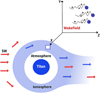 |
Fig. 1 Schematic representation of the SW interaction with Titan and the ion escape via a plasma wakefield that formed behind the test particle. The red arrows show the SW particles, and the blue arrows represent the ionosphere ions. The test particle moves with a velocity parallel to the Z-direction, and the wakefield is formed behind it. The X–Y plane is perpendicular to this motion. |
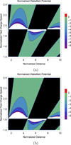 |
Fig. 2 Contour plot of the normalized wakefield potential against the normalized axial distance (z/λD). Panel a shows minimum values, and panel b shows maximum values of the plasma system parameters (see Table 1). In these panels, the attractive potential is represented by the colored regions, whereas the repulsive potential is represented by the black regions. |
Observed data for the plasma parameters in the Titan ionosphere (Whang et al. 2003; Richardson & Smith 2003; Richardson et al. 2004; Garnier et al. 2009).
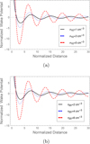 |
Fig. 3 Normalized wakefield potential against the normalized axial distance (z/λD). Panel a shows different n10 with n20 = 5 cm−3, and panel b shows different n20 with n10 = 4 cm−3. Here, n30 = 4 cm−3, nsp0 = nse0 = 5 cm−3, T1 = T2 = T3 = 600 K, Te = 6000 K, Tsp = Tse = 3 × 10⁴ K, usp0 = 400 × 105 cm/s, and the normalized test-charge velocity is equal 1.8. |
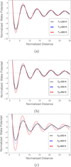 |
Fig. 4 Normalized wakefield potential against the normalized axial distance (z/λD). Panel a shows different T1, panel b shows different T2, and panel c shows different T3. Here, n10 = n30 = 4 cm−3, n20 = 5 cm−3, nsp = nse = 5 cm−3, Te = 6000 K, Tsp = Tse = 3 × 10⁴ K, usp0 = 400 × 105 cm/s, and the normalized test-charge velocity is equal 1.8. |
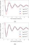 |
Fig. 5 Normalized wakefield potential against the normalized axial distance (z/λD). Panel a shows different nsp0 with nse0 = 5 cm−3, and panel b shows different nse0 with nsp0 = 5 cm−3. Here, n10 = n30 = 4 cm−3, n20 = 5 cm−3, T1 = T2 = T3 = 600 K, Te = 6000 K, Tsp = Tse = 3 × 10⁴ K, usp0 = 400 × 105 cm/s, and the normalized test-charge velocity is equal 1.8. |
 |
Fig. 6 Normalized wakefield potential against the normalized axial distance (z/λD) for different values of usp0. Here, n10 = n30 = 4 cm−3, n20 = 5 cm−3, T1 = T2 = T3 = 600 K, Te = 6000 K, nsp0 = nse0 = 5 cm−3, Tsp = Tse = 3 × 10⁴ K, and the normalized test-charge velocity is equal 1.8. |
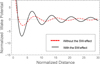 |
Fig. 7 Comparison between the normalized wakefield potential against the normalized axial distance (z/λD) for the existence of the SW (black line) and without the SW (red line). |
4 Summary and conclusion
We proposed a new explanation for the ion-escape process from the upper ionosphere of Titan using an additional mechanism that is known as a test-charge approach. A test particle that exists inside the plasma system is shielded by an opposite-sign charge, leading to the formation of the short-range Debye-Hückel potential around it. When this particle moves, a wakefield potential builds up behind it; this field may be attractive or repulsive. The test particle drags the ionosphere particles through the attractive wakefield. This effect appears when the test-particle velocity is close to the acoustic speed of the ionosphere particle. In other words, all particles in the plasma interact with each other when they have the same velocity ranges. Furthermore, the acoustic speed of the ionosphere particles must exceed the escape velocity of Titan in order to flow out from it. To study the escape process by an attractive wakefield in the upper ionosphere of Titan (1600–1700 km), we therefore constructed our model according to the observed data by the Cassini spacecraft, as well as Voyager 1 and 2. The observed data show that at altitudes from 1600 to 1700 km, there are three dominant species of ions, HCNH+, ![Mathematical equation: $\[\mathrm{C}_{2} \mathrm{H}_{5}^{+}\]$](/articles/aa/full_html/2025/09/aa54191-25/aa54191-25-eq36.png) , and
, and ![Mathematical equation: $\[\mathrm{CH}_{5}^{+}\]$](/articles/aa/full_html/2025/09/aa54191-25/aa54191-25-eq37.png) , and ionosphere electrons (we refer to them with subscripts 1, 2, 3, and e, respectively) that interact with the SW protons (sp) and electrons (se).
, and ionosphere electrons (we refer to them with subscripts 1, 2, 3, and e, respectively) that interact with the SW protons (sp) and electrons (se).
Our results show that the amplitude of the wakefield potential is enhanced when the densities of the ionosphere particles n10 and n20 and their temperatures T1, T2, and T3 are higher. Physically, the denser and warmer plasma system permits an increase in the energy of the ionosphere particles and accelerates them so that they follow the test particles and escape from Titan. The increase in the density of the streaming SW protons nsp0 also increases the amplitude of the wakefield potential, but it is diminished by the increasing electron density nse0. In addition, the numerical result shows that the amplitude of the wakefield potential is not affected by the variation in the velocity of the streaming SW protons usp0 or its temperature Tsp because the solar wind (SW) particles do not significantly interact with the ionosphere particles, as indicated by the observed data. Specifically, the disparity between the SW particle velocity usp0, which ranges from 3 × 10⁷ to 6 × 107 cm/s, and the acoustic speed of the ionosphere plasma, which is approximately 105 cm/s, is large. In other words, the variation in the initial velocity of one of the plasma species affects the collective modes in plasma systems as the velocity scale changes. We also compared the amplitude of the wakefield potential with and without the SW particles. The results indicate that when the SW is present, the amplitude of the attractive field is significantly higher than when the SW is absent. This means that the SW particles pump energy into the system, which accelerates the ions so that they overcome the escape velocity of Titan and escape from it.
Using fast Fourier transform (FFT) power spectra, we determined the characteristics of the ion acoustic waves (IAWs) that exist in the upper ionosphere of Titan in a frequency range of 10–500 Hz with an electric field of (0.5–50) mV/m and with a pulse time duration of (0.01–0.8) s. The previous ranges were determined in addition to the test particles that have maximum potential. The determination of the electric field pulse at a distance of z > 100 λD from the test-charge particle reaches ≈0.05 mV/m, which agrees well with observed data from the Cassini mission, which showed that the range of the electric field pulse at altitudes of 1600–1700 km is ≈0.005–0.06 mV/m. To the best of our knowledge, direct in situ measurements of ion-acoustic waves with electric field amplitudes in the Titan ionosphere are lacking in the range of 0.5–50 mV/m. This constraint largely comes from the limitations in the instrumentation on Cassini, the spaceship that explored Titan. The necessary sensitivity of the apparatus was not built to directly measure an ion-acoustic electric field amplitude this low in this environment. The lack of direct observations therefore restricts our ability to adequately confirm theoretical models with observational data, even though they predict the existence of these waves and their likely influence on the properties of escaping ions. However, our discussion was based on established plasma physics assumptions and similarities with comparable conditions in which ion acoustic waves were observed.
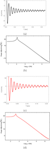 |
Fig. 8 (a) Electric field profile for minimum values of the plasma system parameters (see Table 1) and (b) the FFT power spectra of the electric field. (c) Electric field profile for maximum values of the plasma system parameters (see Table 1). (d) Corresponding FFT power spectra of the electric field. The x-axis signifies the log10 ν, where v is the frequency in Hz, and the y-axis represents the power of the electric field in units of dB(mV/m/Hz). |
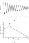 |
Fig. 9 (a) Electric field profile. (b) Corresponding FFT power spectra of the electric field for z > 100 λD from the test-charge particle. Here, n10 = n30 = 2 cm−3, n20 = 3 cm−3, nse0 = nsp0 = 3 cm−3, T1 = T2 = T3= 300 K, Te = 500 K, Tsp = Tse = 2 × 10⁴ K, and usp0 = 300 × 105 cm/s. The x-axis signifies the frequency ν (in Hz), and the y-axis represents the power of the electric field in units of dB(mV/m/Hz). |
Acknowledgements
This study is supported via funding from Prince Sattam bin Abdulaziz University project number (No. PSAU/2025/R/1446).
Appendix Derivation of the wake potential Eq. (18)
Equation (16) can be found from Eq. (14), when we convert the (k, ω) coordinate to (r, t) coordinate using the Fourier transformation, which has the form
![Mathematical equation: $\[\phi_1(\mathbf{r}, ~t)=\frac{1}{(2 \pi)^4} \int\int \phi_1(\mathbf{k}, ~\omega) e^{i(\mathbf{k.} \mathbf{r}-\omega t)} d \omega d k.\]$](/articles/aa/full_html/2025/09/aa54191-25/aa54191-25-eq38.png) (A.1)
(A.1)
Multiplying both sides of Eq. (14) by ![Mathematical equation: $\[\frac{1}{(2 \pi)^{4}} \int\int e^{i(\mathbf{k. r}-\omega t)} d \omega d k\]$](/articles/aa/full_html/2025/09/aa54191-25/aa54191-25-eq39.png) , we can obtain Eq. (16) where at ω = k.vt, the Dirac delta function δ(ω − k.vt) = 1.
, we can obtain Eq. (16) where at ω = k.vt, the Dirac delta function δ(ω − k.vt) = 1.
By using Eq. (15) in Eq. (16), the Debye-Hückel and the wakefield potentials can written as
![Mathematical equation: $\[\phi_D(\mathbf{r}, ~t)=\frac{q_t}{2 \pi^2} \int d k\left(\frac{\lambda_D^2}{k^2 \lambda_D^2+1}\right) e^{i \mathbf{k}.\left(\mathbf{r}-\mathbf{v}_t t\right)},\]$](/articles/aa/full_html/2025/09/aa54191-25/aa54191-25-eq40.png) (A.2)
(A.2)
and
![Mathematical equation: $\[\phi_w(\mathbf{r}, ~t)=\frac{q_t}{2 \pi^2} \int d k\left(\frac{\lambda_D^2}{k^2 \lambda_D^2+1}\right) \frac{\omega_k^2}{\left(\mathbf{k.} \mathbf{v}_t\right)^2-\omega_k^2} e^{i \mathbf{k.}\left(\mathbf{r}-\mathbf{v}_t t\right)},\]$](/articles/aa/full_html/2025/09/aa54191-25/aa54191-25-eq41.png) (A.3)
(A.3)
where
![Mathematical equation: $\[\begin{aligned}\omega_k^2= & \left(\frac{k^2 \lambda_D^2}{k^2 \lambda_D^2+1}\right) \times \\& {\left[\frac{\omega_{p 1}^2}{1-\frac{5}{3} \frac{\left(\mathbf{k.} \mathbf{v}_1\right)^2}{\left(\mathbf{k.} \mathbf{v}_t\right)^2}}+\frac{\omega_{p 2}^2}{1-\frac{5}{3} \frac{\left(\mathbf{k.} \mathbf{v}_2\right)^2}{\left(\mathbf{k.} \mathbf{v}_t\right)^2}}+\frac{\omega_{p 3}^2}{1-\frac{5}{3} \frac{\left(\mathbf{k.} \mathbf{v}_3\right)^2}{\left(\mathbf{k.} \mathbf{v}_t\right)^2}}+\frac{\omega_{p s}^2}{\left[\left(\mathbf{k.} u_{s p 0}\right)^2-\frac{5}{3}\left(\mathbf{k.} v_{s p}\right)^2\right] /\left(\mathbf{k.} \mathbf{v}_t\right)^2}\right]. }\end{aligned}\]$](/articles/aa/full_html/2025/09/aa54191-25/aa54191-25-eq42.png) (A.4)
(A.4)
As a stationary charge forms a Debye shielding as a ball sphere around it (Nambu & Akama 1985; Shukla & Eliasson 2008), we can use a spherical polar coordinate since a stationary to simplify Eq. (A2) to its explicit mathematical expression (Eq. (17)). So that, k=(k sin θk cos ϕk, k sin θk sin ϕk, k cos θk), r=(r sin θr cos ϕr, r sin θr sin ϕr, r cos θr), and vt = (0, 0, vt). Therefore, ![Mathematical equation: $\[\mathbf{k}.(\mathbf{r}-\mathbf{v}_{t} t)=k \rho \sqrt{1-\mu^{2}} ~\cos~ \phi_{k}+k \mu Z\]$](/articles/aa/full_html/2025/09/aa54191-25/aa54191-25-eq43.png) , where ρ(= r sin θr) and Z(= r cos θr − vtt) are the radial and axial distances of an observation point r. Here μ = cos θk and
, where ρ(= r sin θr) and Z(= r cos θr − vtt) are the radial and axial distances of an observation point r. Here μ = cos θk and ![Mathematical equation: $\[\theta_{k}=\sqrt{1-\mu^{2}}\]$](/articles/aa/full_html/2025/09/aa54191-25/aa54191-25-eq44.png) . Then, after some algebraic manipulations, we can obtain the simplest form of the Debye potential in Eq. (17).
. Then, after some algebraic manipulations, we can obtain the simplest form of the Debye potential in Eq. (17).
On the other hand, Eq. (A3) can simplify to obtain Eq. (18) by using a cylindrical coordinate as of the moving charge will proceed with velocity vt in the form of cylinder (Shukla & Eliasson 2008). Then, k.(r − vtt) = k⊥ρ cos ϕk + k∥ζ and dk = k⊥dk⊥k∥dϕk which can obtain
![Mathematical equation: $\[\begin{aligned}\phi_w(\rho, z) & =\frac{q_t}{\pi \lambda_D} \int \frac{J_0\left[K_{\perp} \rho / \lambda_D\right] K_{\perp} d K_{\perp} d K_{\|}}{K_{\perp}^2+K_{\|}^2+1} \exp \left(\frac{i K_{\|} z}{\lambda_D}\right) \\& \times \frac{C_T^2\left(K_{\perp}^2+K_{\|}^2\right)}{\left(K_{\|}-K_{+}\right)\left(K_{\|}+K_{+}\right)\left(K_{\|}^2+K_{-}^2\right) v_t^2},\end{aligned}\]$](/articles/aa/full_html/2025/09/aa54191-25/aa54191-25-eq45.png) (A.5)
(A.5)
where
![Mathematical equation: $\[C_T^2=\left[\frac{\omega_{p 1}^2}{1-5 v_1^2 / 3 v_t^2}+\frac{\omega_{p 2}^2}{1-5 v_2^2 / 3 v_t^2}+\frac{\omega_{p 3}^2}{1-5 v_3^2 / 3 v_t^2}+\frac{\omega_{p s}^2}{\left[u_{s p 0}^2-(5 / 3) v_{s p}^2\right] / v_t^2}\right] \lambda_D^2.\]$](/articles/aa/full_html/2025/09/aa54191-25/aa54191-25-eq46.png) (A.6)
(A.6)
Here, K∥ and K⊥ are parallel and perpendicular components of the dimensionless wavenumber K(= kλD), z = r∥ − vtt. Whereas, J0 represents a zeroth-order Bessel function which tends to unity for small argument, i.e. K⊥ρ/λD < 1. The wake potential in Eq. (A5) generated from the residues at the poles K∥ = ±K+, where ![Mathematical equation: $\[K_{ \pm}^{2}\]$](/articles/aa/full_html/2025/09/aa54191-25/aa54191-25-eq47.png) is written as
is written as
![Mathematical equation: $\[K_{ \pm}^2=\mp \frac{1}{2}\left[1+K_{\perp}^2-\frac{C_T^2}{v_t^2}\right]+\frac{1}{2}\left[\left(1+K_{\perp}^2-\frac{C_T^2}{v_t^2}\right)^2+\frac{2 K_{\perp}^2 C_T^2}{v_t^2}\right]^{1 / 2}.\]$](/articles/aa/full_html/2025/09/aa54191-25/aa54191-25-eq48.png) (A.7)
(A.7)
For K⊥ ≤ 1, K− and K+ may be approximated, respectively as
![Mathematical equation: $\[K_{-} \simeq\left[1-\frac{C_T^2}{v_t^2}\right]^{1 / 2},\]$](/articles/aa/full_html/2025/09/aa54191-25/aa54191-25-eq49.png) (A.8)
(A.8)
and
![Mathematical equation: $\[K_{+}=\frac{C_T K_{\perp}}{v_t}.\]$](/articles/aa/full_html/2025/09/aa54191-25/aa54191-25-eq50.png) (A.9)
(A.9)
Then, after using the expressions of Eqs. (A7)-(A9) into Eq. (A5) and integrating over K⊥ and K∥ we obtain the analytical form of the wakefield potential (Eq. (18)).
References
- Ågren, K., Andrews, D. J., Buchert, S. C., et al. 2011, J. Geophys. Res. Space Phys., 116, A12 [Google Scholar]
- Ågren, K., Edberg, N., & Wahlund, J.-E. 2012, Geophys. Res. Lett., 39, 10 [Google Scholar]
- Ahmed, S., Hassib, E., Abdelsalam, U., Tolba, R., & Moslem, W. 2020, Phys. Plasmas, 27, 082903 [Google Scholar]
- Arridge, C. S., Eastwood, J. P., Jackman, C. M., et al. 2016, Nat. Phys., 12, 268 [Google Scholar]
- Bird, M., Dutta-Roy, R., Asmar, S., & Rebold, T. 1997, Icarus, 130, 426 [Google Scholar]
- Breithaupt, J. 2000, New Understanding Physics for Advanced Level (Oxford University Press: Nelson Thornes) [Google Scholar]
- Coates, A., Crary, F., Lewis, G., et al. 2007, Geophys. Res. Lett., 34, 24 [Google Scholar]
- Coates, A. J., Wellbrock, A., Lewis, G. R., et al. 2012, J. Geophys. Res. Space Phys., 117, A3 [Google Scholar]
- Dubinin, E., Luhmann, J. G., & Slavin, J. A. 2020, Oxford Research Encyclopedia of Planetary Science, 1, (Oxford University Press), 184 [Google Scholar]
- El-Labany, S., Moslem, W., El-Bedwehy, N., Sabry, R., & Abd El-Razek, H. 2012, Astrophys. Space Sci., 338, 3 [Google Scholar]
- El-Shafeay, N., Moslem, W., El-Taibany, W., & El-Labany, S. 2023, Phys. Scrip., 98, 035603 [Google Scholar]
- Garnier, P., Wahlund, J. E., Rosenqvist, L., et al. 2009, Annal. Geophys., 27, 4257 [Google Scholar]
- Goldstein, B. E. 1998, in From the Sun: Auroras, Magnetic Storms, Solar Flares, Cosmic Rays, eds. S. Suess, & B. Tsurutani (Washington: American Geophysical Union (AGU)), 73 [Google Scholar]
- Gosling, J. T. 2014, in Encyclopedia of the Solar System, 3rd edn., eds. T. Spohn, D. Breuer, & T. V. Johnson (Boston: Elsevier), 261 [Google Scholar]
- Gronoff, G., Arras, P., Baraka, S., et al. 2020, J. Geophys. Res. Space Phys., 125, e2019JA027639 [CrossRef] [Google Scholar]
- Johnson, R., Tucker, O., Michael, M., et al. 2010, Titan from Cassini-Huygens (Berlin: Springer), 373 [Google Scholar]
- Moslem, W., Salem, S., Sabry, R., et al. 2019, Astrophys. Space Sci., 364, 1 [NASA ADS] [CrossRef] [Google Scholar]
- Nambu, M., & Akama, H. 1985, Phys. Fluids, 28, 2300 [Google Scholar]
- Regoli, L., Roussos, E., Feyerabend, M., et al. 2016, Planet. Space Sci., 130, 40 [Google Scholar]
- Richardson, J. D., & Smith, C. W. 2003, Geophys. Res. Lett., 30, 5 [Google Scholar]
- Richardson, J. D., Wang, C., & Burlaga, L. 2004, Adv. Space Res., 34, 150 [Google Scholar]
- Salem, S., Moslem, W., & Radi, A. 2017, Phys. Plasmas, 24, 5 [Google Scholar]
- Shen, Y., Knudsen, D. J., Burchill, J. K., et al. 2018, J. Geophys. Res. Space Phys., 123, 3087 [Google Scholar]
- Shukla, P. K., & Eliasson, B. 2008, Phys. Lett. A, 372, 2897 [Google Scholar]
- Strangeway, R., Ergun, R., Su, Y.-J., Carlson, C., & Elphic, R. 2005, J. Geophys. Res. Space Phys., 110, A3 [Google Scholar]
- Strobel, D. F. 2008, Icarus, 193, 588 [Google Scholar]
- Tucker, O. J., & Johnson, R. 2009, Planet. Space Sci., 57, 1889 [Google Scholar]
- Vuitton, V., Lavvas, P., Yelle, R., et al. 2009, Planet. Space Sci., 57, 1558 [NASA ADS] [CrossRef] [Google Scholar]
- Wellbrock, A., Coates, A. J., Jones, G. H., Lewis, G. R., & Waite, J. 2013, Geophys. Res. Lett., 40, 4481 [Google Scholar]
- Westlake, J., Paranicas, C., Cravens, T., et al. 2012, Geophys. Res. Lett., 39, 19 [Google Scholar]
- Whang, Y., Burlaga, L., Wang, Y.-M., & Sheeley Jr, N. 2003, ApJ, 589, 635 [Google Scholar]
- Yahia, M., Tolba, R., & Moslem, W. 2021, Adv. Space Res., 67, 1412 [Google Scholar]
All Tables
Observed data for the plasma parameters in the Titan ionosphere (Whang et al. 2003; Richardson & Smith 2003; Richardson et al. 2004; Garnier et al. 2009).
All Figures
|
Fig. 1 Schematic representation of the SW interaction with Titan and the ion escape via a plasma wakefield that formed behind the test particle. The red arrows show the SW particles, and the blue arrows represent the ionosphere ions. The test particle moves with a velocity parallel to the Z-direction, and the wakefield is formed behind it. The X–Y plane is perpendicular to this motion. |
| In the text | |
|
Fig. 2 Contour plot of the normalized wakefield potential against the normalized axial distance (z/λD). Panel a shows minimum values, and panel b shows maximum values of the plasma system parameters (see Table 1). In these panels, the attractive potential is represented by the colored regions, whereas the repulsive potential is represented by the black regions. |
| In the text | |
|
Fig. 3 Normalized wakefield potential against the normalized axial distance (z/λD). Panel a shows different n10 with n20 = 5 cm−3, and panel b shows different n20 with n10 = 4 cm−3. Here, n30 = 4 cm−3, nsp0 = nse0 = 5 cm−3, T1 = T2 = T3 = 600 K, Te = 6000 K, Tsp = Tse = 3 × 10⁴ K, usp0 = 400 × 105 cm/s, and the normalized test-charge velocity is equal 1.8. |
| In the text | |
|
Fig. 4 Normalized wakefield potential against the normalized axial distance (z/λD). Panel a shows different T1, panel b shows different T2, and panel c shows different T3. Here, n10 = n30 = 4 cm−3, n20 = 5 cm−3, nsp = nse = 5 cm−3, Te = 6000 K, Tsp = Tse = 3 × 10⁴ K, usp0 = 400 × 105 cm/s, and the normalized test-charge velocity is equal 1.8. |
| In the text | |
|
Fig. 5 Normalized wakefield potential against the normalized axial distance (z/λD). Panel a shows different nsp0 with nse0 = 5 cm−3, and panel b shows different nse0 with nsp0 = 5 cm−3. Here, n10 = n30 = 4 cm−3, n20 = 5 cm−3, T1 = T2 = T3 = 600 K, Te = 6000 K, Tsp = Tse = 3 × 10⁴ K, usp0 = 400 × 105 cm/s, and the normalized test-charge velocity is equal 1.8. |
| In the text | |
|
Fig. 6 Normalized wakefield potential against the normalized axial distance (z/λD) for different values of usp0. Here, n10 = n30 = 4 cm−3, n20 = 5 cm−3, T1 = T2 = T3 = 600 K, Te = 6000 K, nsp0 = nse0 = 5 cm−3, Tsp = Tse = 3 × 10⁴ K, and the normalized test-charge velocity is equal 1.8. |
| In the text | |
|
Fig. 7 Comparison between the normalized wakefield potential against the normalized axial distance (z/λD) for the existence of the SW (black line) and without the SW (red line). |
| In the text | |
|
Fig. 8 (a) Electric field profile for minimum values of the plasma system parameters (see Table 1) and (b) the FFT power spectra of the electric field. (c) Electric field profile for maximum values of the plasma system parameters (see Table 1). (d) Corresponding FFT power spectra of the electric field. The x-axis signifies the log10 ν, where v is the frequency in Hz, and the y-axis represents the power of the electric field in units of dB(mV/m/Hz). |
| In the text | |
|
Fig. 9 (a) Electric field profile. (b) Corresponding FFT power spectra of the electric field for z > 100 λD from the test-charge particle. Here, n10 = n30 = 2 cm−3, n20 = 3 cm−3, nse0 = nsp0 = 3 cm−3, T1 = T2 = T3= 300 K, Te = 500 K, Tsp = Tse = 2 × 10⁴ K, and usp0 = 300 × 105 cm/s. The x-axis signifies the frequency ν (in Hz), and the y-axis represents the power of the electric field in units of dB(mV/m/Hz). |
| In the text | |
Current usage metrics show cumulative count of Article Views (full-text article views including HTML views, PDF and ePub downloads, according to the available data) and Abstracts Views on Vision4Press platform.
Data correspond to usage on the plateform after 2015. The current usage metrics is available 48-96 hours after online publication and is updated daily on week days.
Initial download of the metrics may take a while.