| Issue |
A&A
Volume 701, September 2025
|
|
|---|---|---|
| Article Number | A245 | |
| Number of page(s) | 10 | |
| Section | The Sun and the Heliosphere | |
| DOI | https://doi.org/10.1051/0004-6361/202554204 | |
| Published online | 18 September 2025 | |
Three-dimensional magnetic reconnection mediated with plasmoids and the resulting multithermal emissions in the cool atmosphere of the Sun
1
Yunnan Observatories, Chinese Academy of Sciences, Kunming, Yunnan 650216, PR China
2
Max Planck Institute for Solar System Research, Justus-von-Liebig-Weg 3, 37077 Göttingen, Germany
3
University of Chinese Academy of Sciences, Beijing 100049, PR China
4
Yunnan Key Laboratory of Solar Physics and Space Science, Kunming 650216, PR China
5
Institute for Solar Physics (KIS), Georges-Köhler-Allee 401A, 79110 Freiburg, Germany
⋆ Corresponding authors: This email address is being protected from spambots. You need JavaScript enabled to view it.
; This email address is being protected from spambots. You need JavaScript enabled to view it.
Received:
20
February
2025
Accepted:
15
July
2025
Abstract
Context. Flux emergence is ubiquitous in the Sun’s lower atmosphere. The emerging flux can reconnect with the pre-existing magnetic field.
Aims. We aim to investigate plasmoid formation and the resulting multithermal emissions during the three-dimensional reconnection process in the lower solar atmosphere.
Methods. We conducted 3D radiation magnetohydrodynamic (RMHD) simulations using the MURaM code, which incorporates solar convection and radiation. We simulated the emergence of a flat magnetic flux sheet that was introduced into the convection zone. For comparison with results previously reported from observations, we employed the RH1.5D code to synthesize Hα and Si IV spectral line profiles and we synthesized the ultraviolet images using the optical thin methods.
Results. Flux emergence took place as part of the imposed flux tube crossed the photosphere. In the lower solar atmosphere, magnetic reconnection occurred and formed thin, elongated current sheets. Plasmoid-like features appear as part of the reconnection process; this results in many small twisted magnetic flux ropes, which are expelled toward the two ends of the reconnection region. Consequently, hot plasma with a temperature exceeding 20 000 K and much cooler plasmas with a temperature below 10 000 K can coexist in the reconnection region. Synthesized images and spectral line profiles through the reconnection region display typical characteristics of reconnection occuring in the lower solar atmosphere, such as Ellerman bombs (EBs) and UV bursts. The cooler plasmas that show characteristics of EBs can be found above hot plasma and reach altitudes more than 2 Mm above the solar surface. Meanwhile, some hot plasma that features characteristics of UV bursts can extend downward to the lower chromosphere, approximately 0.7 Mm above the solar surface.
Conclusions. Our simulation results indicate that the turbulent reconnection mediated with plasmoid instability can occur in small-scale reconnection events such as EBs and UV bursts. The coexistence of hot and much cooler plasmas in such a turbulent reconnection process can well explain the temporal and spatical connection of UV bursts with EBs.
Key words: magnetic reconnection / Sun: activity / Sun: chromosphere / Sun: magnetic fields
© The Authors 2025
 Open Access article, published by EDP Sciences, under the terms of the Creative Commons Attribution License (https://creativecommons.org/licenses/by/4.0), which permits unrestricted use, distribution, and reproduction in any medium, provided the original work is properly cited.
This article is published in open access under the Subscribe to Open model. This email address is being protected from spambots. You need JavaScript enabled to view it. to support open access publication.
1. Introduction
In the lower solar atmosphere, numerous small-scale brightenings at different wavelengths have been observed (e.g., Katsukawa et al. 2007; Peter et al. 2014; Huang et al. 2017; Toriumi et al. 2017; Young et al. 2018; Joshi & Rouppe van der Voort 2022). Magnetic reconnection is believed to be one of the main mechanisms that drives these events. In the past few decades, many works studied these events, including the characteristics of spectral line profiles and images at different wavelength pass bands (e.g., Fang et al. 2006; Pariat et al. 2007; Peter et al. 2014; Tian et al. 2016; Leenaarts et al. 2025). The corresponding magnetic field structures (e.g., Pariat et al. 2004; Toriumi et al. 2017; Chitta et al. 2017a,b; Samanta et al. 2019) are potentially important to understand their formation process and heating mechanisms.
Limited by the resolution of current observational equipment, further investigation into the fine structures and formation processes of Ellerman bombs (EBs) and UV bursts is significantly challenging. In this context, numerical simulations play a crucial role. Early simulations confirmed that the reconnection processes triggered by U-shaped magnetic field lines, due to Parker instability, are key processes in the formation of EBs (e.g., Isobe et al. 2007; Archontis & Hood 2009). More recent radiative magnetohydrodynamic (RMHD) simulations investigated the formation process of EBs, including the radiative transfer process, from the upper convection zone to the lower solar atmosphere. For instance, Danilovic (2017) utilized the MURaM code (Vögler et al. 2005) to study the reconnection process in the photosphere. Those works (Danilovic 2017) carefully analyzed the whole evolution process, synthesized images and spectral line profiles from different line of sights, and showed the typical characteristics of EBs.
Numerical simulations of magnetic reconnection in the partially ionized low solar atmosphere show that the plasmas can be heated to a high temperature above 20 000 K when the reconnection magnetic field is strong enough and the plasma β is smaller than 0.1 (e.g., Ni et al. 2015, 2016; Peter et al. 2019). The radiation magnetohydrodynamic (RMHD) simulations by Hansteen et al. (2017) studied small-scale magnetic reconnection in the flux emergence region. Their results indicated that the UV bursts are generated in a current sheet that extends from the middle chromosphere to the transition region. However, later simulations by Ni et al. (2022) show that the strong Si IV emissions can also be generated in the lower chromosphere as long as the reconnection magnetic fields are stronger than 500 G. The radiative cooling model used in Ni et al. (2022) is similar to that adopted in Hansteen et al. (2017) for the chromosphere.
Recently, the connection of UV bursts with EBs has been studied in several numerical works. The 3D RMHD simulations by Hansteen et al. (2019) found a vertical current sheet with a hot upper part and a much cooler lower part, which correspond to UV bursts and EBs, respectively. They propose that UV bursts and EBs can be generated in the same reconnection process, but these two brightenings are located at different atmospheric layers and they are far apart from each other (Ortiz et al. 2020). In contrast, Ni et al. (2021) performed high-resolution 2.5D simulations of magnetic reconnection between emerged and background magnetic fields. Their results show that plasmoid instability causes highly nonuniform density distributions in the curved current sheet. The low-density high-temperature (> 20 000 K) and high-density low-temperature (< 10 000 K) plasmas alternatively appear in the space, and the potential hot UV emissions and much cooler Hα wing emissions can be found at approximately the similar height, even within the same plasmoid in the lower chromosphere. The authors’ more recent work further confirmed this model by using the radiative transfer code RH1.5D to synthesize different spectral line profiles and diagnose the different emission sources; the more realistic radiative cooling and ionization effects are included in Cheng et al. (2024a).
There is limited observational evidence of plasmoid instability in the lower solar atmosphere; for example, a few works show blob-like structures in Ca II K and Hα wing images (Rouppe van der Voort et al. 2017, 2024). Recently, Cheng et al. (2024b) identified the plasmoid-like structures at Hα wing images in a small current sheet that were ejected downward to cause the brightenings at the post flare loop region. The turbulent reconnection mediated with plasmoids in the partially ionized low solar atmosphere is presented in many 2D MHD simulations (e.g., Leake et al. 2012; Murphy & Lukin 2015; Ni et al. 2015, 2021; Rouppe van der Voort et al. 2017; Ni & Lukin 2018; Peter et al. 2019; Liu et al. 2023; Wargnier et al. 2023). However, the plasmoid-like structures have never been shown in previous 3D RMHD simulations of EBs and UV bursts (e.g., Hansteen et al. 2017, 2019; Danilovic 2017), except for one recent work by Cheng et al. (2021), which did not include the realistic radiative cooling effect.
In this work, we applied the advanced RMHD code MURaM to investigate magnetic reconnection triggered by flux emergence in the partially ionized lower solar atmosphere. The radiative transfer process results in a realistic plasma and magnetic environment. For the first time, we show that plasmoid instability appears in most of the small-scale reconnection processes relating to EBs and UV bursts in the 3D RMHD simulation. We synthesize the spectral line profiles and images in different wave lengths, and the results further confirm that the hot Si IV emissions and much cooler Hα wing emissions can alternately appear in space in a turbulent reconnection region. The remaining part of this paper is organized as follows. Section 2 introduces the numerical model and initial setups. Section 3 presents the numerical results. The summary and discussion are given in Section 4.
2. Numerical setup
In this study, we utilized the extended MURaM code for our numerical simulations and incorporated capabilities for modeling the coronal and chromospheric extensions. We used theversion described in Rempel (2017), which includes a coronal radiation cooling model and resolves the limitations on time steps caused by high Alfvén speeds, with dissipation settings identical to those described in Przybylski et al. (2022).
The size of the simulation box is 24 Mm × 8 Mm × 12 Mm in the x, y, and z directions, respectively, with the z axis perpendicular to the solar surface. The upper convection zone extends from z = −4 Mm to z = 0 Mm, and the solar atmospheric region extends from z = 0 Mm to z = 8 Mm. The grid size in the x direction is 23.4 km, and it is 15.63 km in y and z direction. The grid number is 1024 × 512 × 768. This resolution is adequate for resolving the small structures within current sheets, even though it is still much lower than that in our previous 2D simulations in which we employed adaptive mesh refinement (AMR) technology (e.g., Ni et al. 2021; Cheng et al. 2024a).
In our simulations, we used the local thermodynamic equilibrium (LTE) radiative cooling model for the photosphere and lower chromosphere, and the optically thin radiative cooling model was applied for the upper chromosphere and corona region. We began with a convecting simulation that extends to z = 2 Mm. We insert a magnetic flux sheet at z = −2 Mm and the peak strength was 2200 G. The strength of the magnetic field decreases with height, and the effective radius is about 0.5 Mm. The convection motions cause the magnetic fields to emerge upward into the solar atmosphere.
When the system reaches a relaxed state, we extend the simulation into the region above z = 2 Mm. The magnetic fields from z = 2 Mm to z = 8 Mm at the beginning of the second stage are given by the potential extrapolation method, while the initial temperature is expanded into the corona region by using a tanh function to match to a coronal temperature of 106 K. The initial density and internal energy distributions are derived from the hydrostatic assumption. The velocity above z = 2 Mm is set to zero at the beginning of the second stage. Subsequently, we run the simulation for about 1.25 solar hours to study the small-scale reconnection events during this stage.
Periodic boundary conditions are applied in both the x and y directions. The upper boundary condition is semi-open, allowing only outflows and prohibiting inflows, with a hot plane set at a temperature of 106 K. The bottom boundary permits both outflows and inflows, utilizing an isentropic lower boundary condition. The magnetic fields at the upper boundary are determined by potential field extrapolation. To quickly form a layer with coronal temperatures in the top region, we enabled the hot-plane option. The magnetic fields at the bottom boundary adopt symmetric magnetic components; this is termed open-boundary symmetric-field OSb, as described in Rempel (2014). The state equation used in the simulation is the Uppsala equation (Gudiksen et al. 2011). During our focus period, raw data were saved at five-second intervals for the subsequent analysis of reconnection events.
3. Results
3.1. Turbulent reconnection mediated with plasmoids
After extending the simulation domain and running the MURaM code for over one solar hour, the turbulent convective cells in the convection zone and the irregular movement of granules in the photosphere cause magnetic flux to emerge into the atmosphere, which forms complex and diverse magnetic field structures. In some regions, magnetic fields with opposite polarities approach each other and reconnection appears. Due to the high spatial resolution in this simulation, the region between 0 and 4 Mm above the photosphere is filled with many small-scale magnetic reconnection events. Turbulent reconnection mediated with plasmoid instability appears in most of these reconnection events. Small twisted magnetic flux ropes or plasmoids are formed in such events, with sizes typically ranging from a few hundred kilometers to about 1 Mm and occurring as low as around z = 1 Mm. They are ejected downward and upward with the bidirectional flows. Therefore, a portion of the twisted flux ropes are transported to the higher atmosphere.
Figure 1 is a 3D overview of the simulation area at t = 4414 seconds. The grayscale image at the bottom represents the longitudinal magnetic field at the solar surface, the colored lines represent the magnetic field lines in the simulation area, while the red-to-yellow isosurfaces represent the regions where the temperature is higher than 20 000 K. We see that the local regions have been heated to such a high temperature in many of the small-scale reconnection events. Here, we focus on a reconnection event near the left surface as shown in the purple box in Fig. 1, which is located around x = 2 Mm, y = 4 Mm, and extends from z = 1 Mm to z = 5.5 Mm in the z direction; this is our primary region of interest (ROI). This reconnection region appears as a curved, elongated structure resembling a sausage, with an uneven distribution of high-temperature components. The blob-like features are visible and indicate the occurrences of plasmoid instability in this reconnection event.
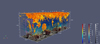 |
Fig. 1. Three-dimensional overview of the simulation domain above the photosphere at t = 4414 s. The colored line structures represent the magnetic field lines in the simulation area, with colors corresponding to the field strengths. The grayscale slice at the bottom illustrates the distribution of the longitudinal magnetic field at the solar surface. Yellow and red isosurfaces represent the regions where temperatures are above 20 000 K. The purple box represents the region of interest. More details can be found in the supplementary online. |
Figure 2 displays the distributions of temperature and longitudinal magnetic field (Bz) in the x − z slices at y = 4.3 Mm at three different times. The Bz distribution shown in panels b, d, and f indicates that the local reconnection events are abundant in this plane. In particular, the elongated reconnection region between x = 0.5 Mm and x = 2.5 Mm (which corresponds to the ROI) is notable, as shown in panels a, c, and e. At t = 4301 s, no significant plasmoids appear and the temperature in the reconnection area does not exceed 20 000 K. At t = 4414 s, Fig. 2c shows clear plasmoid structures and highly nonuniform temperature distributions in the ROI, with the highest temperature in this region exceeding 90 000 K. At t = 4489 s, we can see that the plasmoid structures become obscure again, and some of the high-temperature regions disappear.
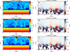 |
Fig. 2. Slices at y = 4.3 Mm at three different times in the simulation. The left column displays the temperature distribution in the slice planes, while the right column shows the distribution of the magnetic field strength (Bz) perpendicular to the solar surface. More details can be found in the supplementary online. |
Figure 3 further illustrates the presence of plasmoid instability in the ROI with slices cut through different directions and locations. Figure 3a displays the distribution of the longitudinal magnetic field at the solar surface, which is primarily influenced by the turbulent movement of granular structures; the magnetic fields converge in the intergranular lanes, with the strongest field strengths exceeding 1500 G. We observe that positive and negative magnetic fields approach each other at many different locations. The ROI is located above the position near x = 2 Mm and y = 4 Mm, where small-scale positive and negative magnetic fields exist. The distribution of plasma temperature, density, and current density in two x-direction slices (S1, S2) and a y-direction slice (S3) at t = 4414 s are presented in Figs. 3b–i; these slices pass through the ROI. The elongated current sheet in the ROI is very turbulent and mediated with plasmoids in these planes. The plasmas with different temperatures and densities appear alternately in the reconnection region. We can see that the cool plasma below 10 000 K can even appear above the hot plasma that exceeds 20 000 K, as show for example, by the big, relatively cooler blob that passes by the blue arrow in Figs. 3b and 3d. These phenomena are very similar to previous two-dimensional simulations (e.g., Ni et al. 2021; Cheng et al. 2024a) where plasmoids appeared as magnetic islands, but in the three-dimensional simulation, they correspond to magnetic flux ropes. We can also see that the current sheet extends to higher heights than in previous two-dimensional (Ni et al. 2021; Cheng et al. 2024a) simulations (reaching up to y = 6 Mm), with the background plasma density much lower. However, thecurrent sheet is still filled with high-density plasma up to 1019 m−3, and a large amount of high-density plasma is pushed into the reconnection region or even reaches above the current sheet during the magnetic flux emergence process, which suggest the possible occurrence of EBs at higher heights.
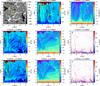 |
Fig. 3. Slices along different directions at t = 4414 s in the simulation. Panel a illustrates the longitudinal magnetic field (Bz) at the solar surface, marked with dashed lines to indicate the positions of slices S1, S2, and S3. Panels b and c represent the temperature and density distributions along slice S3 within the y − z plane. Panels d to f and panels g to i respectively show the temperature, density, and current density (Jz) distributions along slices S1 and S2 in the x − z plane. The black curves in the figure indicate the height at which the Hα line center optical depth equals unity. |
The 3D distributions of magnetic field lines and plasmas with higher and lower temperatures mixed in the ROI are presented in Fig. 4. Panels a and b show that multiple twisted magnetic flux ropes that correspond to plasmoids are generated in the reconnection region, and those upward moving flux ropes unravel and interact with the open field. The red isosurfaces in panels c and d represent the high-temperature regions (above 20 000 K), and the green isosurfaces correspond to the low-temperature regions (below 8000 K). We find that the high- and low-temperature regions are intertwined within the current sheet. High temperatures above 20 000 K also appear in reconnection outflow regions. The fragmented high-temperature regions in the current sheet and outflows further indicate the appearance of turbulent reconnection. Additionally, the supplementary movie shows some twisted magnetic ropes entering higher atmospheric layers with the outflows. Moreover, we find arch-like magnetic field structures below the reconnection current sheet that resemble post reconnection loops, but the temperature in this region does not exceed 20 000 K.
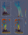 |
Fig. 4. Three-dimensional views of the interesting region at t = 4414 s. The grayscale image at the bottom represents the longitudinal magnetic field at the solar surface. Lines with different colors indicate magnetic field lines. The red isosurfaces indicate the regions with high-temperature plasma, while green isosurfaces represent low-temperature regions. Panel b is a zoomed-in view of the reconnected region in panel a. More details can be found in the supplementary online. |
3.2. Radiation characteristics of reconnection events
We utilized the RH1.5 code (Pereira & Uitenbroek 2015) to synthesize the spectral line profiles and images in the Hα and Si IV pass bands in order to further study the reconnection activities and more effectively compare them with observations. RH1.5D solves the radiative transfer processes column by column in the three-dimensional simulation region and treats the three-dimensional atmosphere as a 1.5-dimensional distribution to save computational resources. Since computing the Si IV emission requires a complex model of the Si atom, using the RH1.5D code to calculate the radiative characteristics of Si IV 139.4 nm for the entire simulation region involves a substantial computational cost. Therefore, we primarily employed the optically thin assumption combined with the CHIANTI atomic database (Dere et al. 1997) to synthesize the images in Si IV 139.4 nm and EUI (Solar Orbiter/Extreme Ultraviolet Imager) 17.4 nm. However, the Si IV spectral line profiles are synthesized using the RH1.5 code.
Figures 2, 3, and 4 reveal the multithermal structures of magnetic reconnection in the ROI. The temperature increase in the low-temperature region is only in the range of hundreds to thousands of kelvins and plasma density in this region ranges from 10−10 to 10−9 g cm−3; these conditions are highly conducive for the formation of EBs. The highest temperatures in the current sheet can approach 90 000 K and the high-temperature regions that exceed 20 000 K are very likely to have strong UV emissions. The conditions for the formation of EBs and UV bursts are simultaneously satisfied within a multithermal reconnection current sheet. To verify whether both EBs and UV bursts coexist in the same current sheet, we firstly used the RH1.5D code to synthesize the images in the Hα wing along the z direction at t = 4414 s. Additionally, we also synthesized images in the Si IV 139.4 nm and EUI 17.4 nm by using the optically thin method, with the line-of-sight direction perpendicular to the solar surface (z direction). The results are presented in Fig. 5. Panel a displays a synthetic image near Hα −0.5 Å that clearly shows there are many noticeable brightenings in the simulation domain. The UV emission in Si IV 139.4 nm is also significant in many tiny regions, as shown in panel b. However, panel c indicates that the extreme ultraviolet emissions are not obvious in the whole domain, especially within the ROI. The ROI is within the dashed red box near the left boundary in panels a and b.
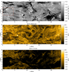 |
Fig. 5. Synthetic observables from a line of sight oriented vertically to the solar surface at t = 4414 s in the simulation. Panel a displays the Hα wing radiation at the Hα −0.5 Å wavelength calculated by using the RH1.5D code. Panel b shows the Si IV 139.4 nm synthetic radiation image calculated by using the optically thin method. Panel c presents the synthetic image of the EUI 17.4 nm band, also calculated by using the optically thin method. Hereafter, IR denotes the relative radiation intensity. |
Figure 6 shows the zoomed-in pictures of the synthetic images in the Hα wing and Si IV 139.4 nm within the dashed red box plotted in Fig. 5. The regions with obvious Hα wing emissions are highlighted by the blue isolines in panel a. The green isolines in panels a and b are used to mark the regions with significant Si IV emissions. The long curved reconnection region with multiple plasmoids and multithermal structures as shown in Figs. 2, 3, and 4 is located from x = 0 Mm to x = 2.5 Mm and from y = 3.5 Mm to y = 5 Mm. In this region, we see that some areas within the blue isolines overlap with or are close to the areas within the green isolines, which indicates the possible appearances of UV bursts connecting with EBs.
Assuming the dashed red line in Fig. 6a represents the slit of a spectrograph, we synthesized the Hα spectral image for the slit as shown in Fig. 7a. Its main features are similar to those observed by Ellerman (1917), with no obvious radiations at the Hα line center but significant emission enhancements in the Hα blue and red wings. In Fig. 7b, we show the temperaturedistribution in the y − z plane along the dashed red line in Fig. 6, and the gray line in this plane represents the location where the optical depth of the Hα wing (−0.5 Å) equals unit. Fig. 7c shows the vertical velocity distribution in the same plane, with the maximum velocity in the z direction reaching up to 70 km s−1. Figure 7d presents the Si IV emission intensity synthesized using the optically thin approximation. One can see that the regions with strong Si IV emissions in Fig. 7d correspond well to the regions with high-temperature plasmas in Fig. 7b. These high-temperature plasmas are mostly located below the gray line in Fig. 7b, which indicates they are at a lower chromosphere.
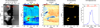 |
Fig. 7. Panel a: Synthetic Hα spectrum at t = 4414 s. The image displays the synthesized spectrum for comparison with Ellerman’s observations from 1917, with the horizontal axis representing wavelength and the vertical axis representing the length along the dashed red line in Fig. 6. The dashed red line in Fig. 6a acts as an imaginary spectrograph slit. Panels b to d present physical quantities in the y − z plane along the dashed red line indicated in Fig. 6. In panel b, the temperature distribution is shown, with the gray and black lines representing the locations where the optical depths of the Hα wing (−0.5 Å) and Hα line center reach unity, respectively. Panel c displays the vertical velocity (vz) distribution, panel d shows the emissivity of Si IV, and panel e displays the synthesized Si IV spectral line profile calculated from the blue rectangular region marked in Fig. 6b. |
We also used the RH1.5D to calculate the averaged Si IV spectral line profile in the small blue box of Fig. 6b, with the line of sight along the z direction. The result is shown in Fig. 7e. The Si IV 139.4 nm line profile in this area exhibits a distinct double-peaked emission structure, and the spectral line width exceeds 70 km s−1. These results match the main observational features of UV bursts. The simulation results also suggest that the reconnection downward outflows can reach a speed of 100 km s−1, and upward outflows approximately reach 80 km s−1, which is consistent with the recent observational results of small-scale events in the lower solar atmosphere (e.g., Leenaarts et al. 2025).
The above analyses about the radiation characteristics of the target reconnection event in the ROI further demonstrate that the UV busts and EBs coexist in a single reconnection event. Multithermal plasmas with different temperatures caused by the turbulent reconnection process contribute emissions in different pass bands. In addition to this target event, there are many other reconnection events in the whole simulation domain. Some of them exhibit even stronger radiative signatures. However, this particular event shows more well-identified plasmoid structures.
3.3. The formation height of EBs and UV bursts
The current sheet presented in Fig. 3 displays a complex multithermal structure. We can see a distinct low-temperature (< 10 000 K) plasma blob located on the right hand side of the curved current sheet, with its center near x = 1.8 Mm and y = 3 Mm. The evident high-temperature (> 20 000 K) current sheet fragments are located below this cooler plasma blob. However, we also notice that the temperature of this blob is still higher than the surrounding environment. As shown in Fig. 8, we calculated the averaged Hα-pagination line profiles along the z direction through this plasma blob (marked by the blue arrows in Figs. 3b and d), with specific calculations performed inside the small blue box in Fig. 3a. In Fig. 8, the Hα line profile shows distinct bulges on both wings that deviate from a Gaussian profile, which indicates enhanced radiation in the wings. Figure 8b displays the Hα line profile after subtracting the nearby background profile, which also shows enhancements in the wings, though the enhancement at the line center is very weak. Therefore, this plasma blob exhibits clear EB characteristics, which are located above some high-temperature areas of the current sheet. These results imply that in a magnetic reconnection event where both EBs and UV bursts occur simultaneously, the location of the much cooler EBs can be at a higher height than the hot UV emission.
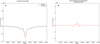 |
Fig. 8. Hα spectral line profiles through the low-temperature plasma blob indicated by the blue arrows in Figs. 3a and d. Panel a shows the spectral line profile calculated using RH1.5D directly, and panel b shows the result after subtracting the background spectral line profile. |
Such kinds of reconnection events with multithermal structures frequently appear in the whole simulation, and hot plasmas with strong UV emissions can be located at a very low height. Figure 9 shows a slice of another magnetic reconnection event at t = 4548 s, with Panels a, b, c, and d displaying the longitudinal magnetic field (Bz), temperature distribution, longitudinal velocity (Vz), and density distribution, respectively. The figures reveal that high-temperature plasma that exceeds 20 000 K appears in a typical low chromospheric environment at about 0.7 Mm above the solar surface. The density in most of the reconnection region is significantly higher than the background, except for the high-temperature area. The Bz at the bottom of this reconnection region is about 300 G, with a total magnetic field strength of about 500 G. Panel e shows the Si IV spectral line profile along the z direction calculated by RH1.5D for this region, which also exhibits a double-peaked structure. The Doppler width of the line is around 50 km s−1, and its radiation intensity is significantly higher than that shown in Fig. 7e; this is attributed to the considerably higher density in this reconnection event. Panel f shows the results of the synthetic image in Si IV viewed along the y direction, passing through the high-temperature plasma area of the reconnection. The reconnection current sheet shows a distinct response in the Si IV band, which presents as a slender bright band structure, similar to the flame-like structures commonly observed. Such a result demonstrates that UV bursts can appear in the lower chromosphere as long as the reconnection magnetic fields are strong enough, which is consistent with previous 2D simulation results (Ni et al. 2016, 2022; Ni & Lukin 2018; Cheng et al. 2024a).
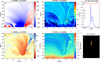 |
Fig. 9. Slices at t = 4548 s and y = 2.61 Mm of another reconnection event. The figure displays the distribution of the magnetic field in the z direction, temperature, velocity in the z direction (Vz), density, the synthesized Si IV spectral line profile, and the synthetic image of the high-temperature area in the Si IV band along the y direction. |
4. Conclusions and discussions
We conducted a high-resolution, three-dimensional RMHD simulation using the MURaM code, covering the upper convection zone to the lower corona. In this simulation, the magnetic field is shaped by the irregular motions of convective cells and photospheric granules, and these magnetic fields rise from the convection zone into the solar atmosphere and subsequently formvarious dynamic structures. High-density plasma (> 1019 m−3) in the lower atmosphere also ascends to higher layers with the emerged magnetic field. Throughout the simulation, frequent appearances of magnetic structures with opposite polarities were observed that led to many small-scale magnetic reconnection events. The high resolution enabled fine plasma structures within reconnection current sheets to be captured and facilitated observations of nonuniform distributions of density and temperature. We tracked the evolution of a target region (ROI) and used the RH1.5D code and the optically thin radiation approximation model to synthesize radiation images and spectral line profiles for Hα, Si IV 139.4 nm, and EUI 17.4 nm. This led to several important conclusions:
-
In the simulation, most small-scale reconnections led to the formation of twisted magnetic flux ropes in the reconnection regions that resembled plasmoids. Some of these flux ropes, driven by bi-directional flows, move upward away from the solar surface, carrying twisted magnetic fields into the upper layers of the solar corona. Additionally, the magnetic topology of the reconnection process seen in the targeted event resembles that found in large-scale solar flare models.
-
The turbulent magnetic reconnection process leads to highly nonuniform distributions of density and temperature in the reconnection regions, where plasmas with different temperatures alternately appear in space. A part of the plasma in these reconnections is heated to above 20 000 K, with peak temperatures reaching 90 000 K. This high-temperature plasma generates strong Si IV ultraviolet radiation. In contrast, cooler regions of the reconnection processes cause a significant enhancement in the Hα line wing radiation. The synthesized spectral line profiles and imaging results in the Hα and Si IV bands through the targeted reconnection region indicate the coexistence of EBs and UV bursts during this magnetic reconnection process.
-
In the turbulent magnetic reconnection events that involve a mixture of high and low temperatures, cool plasma that displays characteristics of EBs can be found above hot plasma and can reach altitudes more than 2 Mm above the solar surface. Meanwhile, some high-temperature plasma that features characteristics of UV bursts can extend downwards to the lower chromosphere, approximately 0.7 Mm above the solar surface.
Our analysis of the targeted event suggests that the multithermal turbulent current sheet structures caused by plasmoid instability can plausibly explain the formation mechanisms of UV bursts connecting with EBs, which further validates the model we previously proposed in two-dimensional simulations (Ni et al. 2021; Cheng et al. 2024a). The reconnection structures presented in the three-dimensional simulation are significantly more complex. We should also point out that plasmoid instability can only occur when the aspect ratio of the current sheet or the Lundquist number exceeds a critical value (e.g., Ni et al. 2012; Leake et al. 2012). The lower solar atmosphere is normally very dynamic and the current sheet aspect ratio can vary with time; then plasmoid instability might only last for a while and then disappear.
The magnetic field strength in the target event region approximately ranges from 150 G to 250 G, and it decreases with height, which is similar to what we found in our previous 2D work in Cheng et al. (2024a). Such a curved current sheet extending from the lower atmosphere to the higher altitude is significantly different from the horizontal current sheet in Ni et al. (2022). The initial uniform plasma density in Ni et al. (2022) is about 1021 m−3 (comparable to the density in the solar temperature minimum region), and it is more than ten times higher than that in the target reconnection region in this work. Therefore, the reconnection magnetic field must be a higher strength (≳500 G) to heat the denser plasma there to a temperature above 20 000 K, as shown in Ni et al. (2022).
The simulation results also indicate that the turbulent reconnection mediated by plasmoids is widespread in the lower solar atmosphere and may play an important role in nonhomogeneously heating the atmosphere. In particular, if elongated current sheets with lengths of 2−3 Mm or more can persist for some time under low plasma-beta conditions, as are readily achieved in this simulation. Recent high-resolution observations have revealed the complex nonuniform thermal structure of the lower solar atmosphere (e.g., Peter et al. 2014), where the turbulent reconnection mediated by plasmoids may play a significant role. As we know, plasmoid-like structures have been frequently observed in the large-scale current sheet related to solar flares. In our target reconnection event, the magnetic topology resembles that of the standard flare model, which suggests potential similarities between these events at different scales. Despite differences in formation locations and scales, they may share similar triggering mechanisms and an underlying physical model.
Finally, we point out some of the limitations in our study. For instance, the height in the z direction is set to 8 Mm above the solar surface. As the magnetic flux emergence process continues, a substantial amount of high-density plasma is transported to higher altitudes and pushes the original coronal material out through the upper boundary. This results in only a small amount of coronal material near the upper boundary of the simulation area. In future work, it will be necessary to optimize this aspect to ensure the simulation region encompasses a more extensive coronal plasma environment and better models the actual conditions of the Sun.
Data availability
Movies associated with Figs. 1, 2, 4 are available at https://www.aanda.org
Acknowledgments
This research is supported by the Strategic Priority Research Program of the Chinese Academy of Sciences with Grant No. XDB0560000; the National Key R & D Program of China No. 2022YFF0503003 (2022YFF0503000); the National Key R & D Program of China No. 2022YFF0503804 (2022YFF0503800); the NSFC Grants 12373060 and 11933009; the outstanding member of the Youth Innovation Promotion Association CAS (No. Y2021024); the Basic Research of Yunnan Province in China with Grant 202401AS070044; the Yunling Talent Project for the Youth; the Yunling Scholar Project of the Yunnan Province and the Yunnan Province Scientist Workshop of Solar Physics; the International Space Science Institute (ISSI) in Bern, through ISSI International Team project # 23-586 (Novel Insights Into Bursts, Bombs, and Brightenings in the Solar Atmosphere from Solar Orbiter); Yunnan Key Laboratory of Solar Physics and Space Science under the number 202205AG070009; The numerical calculations and data analysis have been done on Max Planck Computing and Data Facility and on the Computational Solar Physics Laboratory of Yunnan Observatories.
References
- Archontis, V., & Hood, A. W. 2009, A&A, 508, 1469 [NASA ADS] [CrossRef] [EDP Sciences] [Google Scholar]
- Cheng, G.-C., Ni, L., Chen, Y.-J., et al. 2021, RAA, 21, 229 [Google Scholar]
- Cheng, G., Ni, L., Chen, Y., et al. 2024a, A&A, 685, A2 [NASA ADS] [CrossRef] [EDP Sciences] [Google Scholar]
- Cheng, G., Ni, L., Tang, Z., et al. 2024b, ApJ, 966, L29 [NASA ADS] [CrossRef] [Google Scholar]
- Chitta, L. P., Peter, H., Solanki, S. K., et al. 2017a, ApJS, 229, 4 [Google Scholar]
- Chitta, L. P., Peter, H., Young, P. R., et al. 2017b, A&A, 605, A49 [NASA ADS] [CrossRef] [EDP Sciences] [Google Scholar]
- Danilovic, S. 2017, A&A, 601, A122 [NASA ADS] [CrossRef] [EDP Sciences] [Google Scholar]
- Dere, K. P., Landi, E., Mason, H. E., et al. 1997, A&AS, 125, 149 [NASA ADS] [CrossRef] [EDP Sciences] [Google Scholar]
- Ellerman, F. 1917, ApJ, 46, 298 [NASA ADS] [CrossRef] [Google Scholar]
- Fang, C., Tang, Y. H., Xu, Z., et al. 2006, ApJ, 643, 1325 [NASA ADS] [CrossRef] [Google Scholar]
- Gudiksen, B. V., Carlsson, M., Hansteen, V. H., et al. 2011, A&A, 531, A154 [NASA ADS] [CrossRef] [EDP Sciences] [Google Scholar]
- Hansteen, V. H., Archontis, V., Pereira, T. M. D., et al. 2017, ApJ, 839, 22 [NASA ADS] [CrossRef] [Google Scholar]
- Hansteen, V., Ortiz, A., Archontis, V., et al. 2019, A&A, 626, A33 [NASA ADS] [CrossRef] [EDP Sciences] [Google Scholar]
- Huang, Z., Madjarska, M. S., Scullion, E. M., et al. 2017, MNRAS, 464, 1753 [NASA ADS] [CrossRef] [Google Scholar]
- Isobe, H., Tripathi, D., & Archontis, V. 2007, ApJ, 657, L53 [NASA ADS] [CrossRef] [Google Scholar]
- Joshi, J., & Rouppe van der Voort, L. H. M. 2022, A&A, 664, A72 [NASA ADS] [CrossRef] [EDP Sciences] [Google Scholar]
- Katsukawa, Y., Berger, T. E., Ichimoto, K., et al. 2007, Science, 318, 1594 [NASA ADS] [CrossRef] [Google Scholar]
- Leake, J. E., Lukin, V. S., Linton, M. G., et al. 2012, ApJ, 760, 109 [NASA ADS] [CrossRef] [Google Scholar]
- Leenaarts, J., van Noort, M., de la Cruz Rodríguez, J., et al. 2025, A&A, 696, A3 [NASA ADS] [CrossRef] [EDP Sciences] [Google Scholar]
- Liu, R. 2020, RAA, 20, 165 [Google Scholar]
- Liu, M., Ni, L., Cheng, G.-C., et al. 2023, RAA, 23, 035006 [NASA ADS] [Google Scholar]
- Murphy, N. A., & Lukin, V. S. 2015, ApJ, 805, 134 [Google Scholar]
- Ni, L., & Lukin, V. S. 2018, ApJ, 868, 144 [Google Scholar]
- Ni, L., Ziegler, U., Huang, Y.-M., et al. 2012, Phys. Plasmas, 19, 072902 [NASA ADS] [CrossRef] [Google Scholar]
- Ni, L., Kliem, B., Lin, J., et al. 2015, ApJ, 799, 79 [NASA ADS] [CrossRef] [Google Scholar]
- Ni, L., Lin, J., Roussev, I. I., et al. 2016, ApJ, 832, 195 [NASA ADS] [CrossRef] [Google Scholar]
- Ni, L., Chen, Y., Peter, H., et al. 2021, A&A, 646, A88 [NASA ADS] [CrossRef] [EDP Sciences] [Google Scholar]
- Ni, L., Cheng, G., & Lin, J. 2022, A&A, 665, A116 [NASA ADS] [CrossRef] [EDP Sciences] [Google Scholar]
- Ortiz, A., Hansteen, V. H., Nóbrega-Siverio, D., et al. 2020, A&A, 633, A58 [NASA ADS] [CrossRef] [EDP Sciences] [Google Scholar]
- Pariat, E., Aulanier, G., Schmieder, B., et al. 2004, ApJ, 614, 1099 [Google Scholar]
- Pariat, E., Schmieder, B., Berlicki, A., et al. 2007, A&A, 473, 279 [NASA ADS] [CrossRef] [EDP Sciences] [Google Scholar]
- Pereira, T. M. D., & Uitenbroek, H. 2015, A&A, 574, A3 [NASA ADS] [CrossRef] [EDP Sciences] [Google Scholar]
- Peter, H., Tian, H., Curdt, W., et al. 2014, Science, 346, 1255726 [Google Scholar]
- Peter, H., Huang, Y.-M., Chitta, L. P., et al. 2019, A&A, 628, A8 [NASA ADS] [CrossRef] [EDP Sciences] [Google Scholar]
- Przybylski, D., Cameron, R., Solanki, S. K., et al. 2022, A&A, 664, A91 [NASA ADS] [CrossRef] [EDP Sciences] [Google Scholar]
- Rempel, M. 2014, ApJ, 789, 132 [Google Scholar]
- Rempel, M. 2017, ApJ, 834, 10 [Google Scholar]
- Rouppe van der Voort, L., De Pontieu, B., Scharmer, G. B., et al. 2017, ApJ, 851, L6 [Google Scholar]
- Rouppe van der Voort, L. H. M., Joshi, J., Henriques, V. M. J., et al. 2021, A&A, 648, A54 [NASA ADS] [CrossRef] [EDP Sciences] [Google Scholar]
- Rouppe van der Voort, L. H. M., Joshi, J., & Krikova, K. 2024, A&A, 683, A190 [NASA ADS] [CrossRef] [EDP Sciences] [Google Scholar]
- Samanta, T., Tian, H., Yurchyshyn, V., et al. 2019, Science, 366, 890 [NASA ADS] [CrossRef] [Google Scholar]
- Shen, Y. 2021, Proc. Roy. Soc. London Ser. A, 477, 217 [NASA ADS] [Google Scholar]
- Tian, H., Xu, Z., He, J., et al. 2016, ApJ, 824, 96 [CrossRef] [Google Scholar]
- Toriumi, S., Katsukawa, Y., & Cheung, M. C. M. 2017, ApJ, 836, 63 [Google Scholar]
- Vögler, A., Shelyag, S., Schüssler, M., et al. 2005, A&A, 429, 335 [Google Scholar]
- Wargnier, Q. M., Martínez-Sykora, J., Hansteen, V. H., et al. 2023, ApJ, 946, 115 [NASA ADS] [CrossRef] [Google Scholar]
- Young, P. R., Tian, H., Peter, H., et al. 2018, Space Sci. Rev., 214, 120 [Google Scholar]
All Figures
|
Fig. 1. Three-dimensional overview of the simulation domain above the photosphere at t = 4414 s. The colored line structures represent the magnetic field lines in the simulation area, with colors corresponding to the field strengths. The grayscale slice at the bottom illustrates the distribution of the longitudinal magnetic field at the solar surface. Yellow and red isosurfaces represent the regions where temperatures are above 20 000 K. The purple box represents the region of interest. More details can be found in the supplementary online. |
| In the text | |
|
Fig. 2. Slices at y = 4.3 Mm at three different times in the simulation. The left column displays the temperature distribution in the slice planes, while the right column shows the distribution of the magnetic field strength (Bz) perpendicular to the solar surface. More details can be found in the supplementary online. |
| In the text | |
|
Fig. 3. Slices along different directions at t = 4414 s in the simulation. Panel a illustrates the longitudinal magnetic field (Bz) at the solar surface, marked with dashed lines to indicate the positions of slices S1, S2, and S3. Panels b and c represent the temperature and density distributions along slice S3 within the y − z plane. Panels d to f and panels g to i respectively show the temperature, density, and current density (Jz) distributions along slices S1 and S2 in the x − z plane. The black curves in the figure indicate the height at which the Hα line center optical depth equals unity. |
| In the text | |
|
Fig. 4. Three-dimensional views of the interesting region at t = 4414 s. The grayscale image at the bottom represents the longitudinal magnetic field at the solar surface. Lines with different colors indicate magnetic field lines. The red isosurfaces indicate the regions with high-temperature plasma, while green isosurfaces represent low-temperature regions. Panel b is a zoomed-in view of the reconnected region in panel a. More details can be found in the supplementary online. |
| In the text | |
|
Fig. 5. Synthetic observables from a line of sight oriented vertically to the solar surface at t = 4414 s in the simulation. Panel a displays the Hα wing radiation at the Hα −0.5 Å wavelength calculated by using the RH1.5D code. Panel b shows the Si IV 139.4 nm synthetic radiation image calculated by using the optically thin method. Panel c presents the synthetic image of the EUI 17.4 nm band, also calculated by using the optically thin method. Hereafter, IR denotes the relative radiation intensity. |
| In the text | |
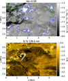 |
Fig. 6. Synthetic observables in the dashed-red rectangular area of Fig. 5. |
| In the text | |
|
Fig. 7. Panel a: Synthetic Hα spectrum at t = 4414 s. The image displays the synthesized spectrum for comparison with Ellerman’s observations from 1917, with the horizontal axis representing wavelength and the vertical axis representing the length along the dashed red line in Fig. 6. The dashed red line in Fig. 6a acts as an imaginary spectrograph slit. Panels b to d present physical quantities in the y − z plane along the dashed red line indicated in Fig. 6. In panel b, the temperature distribution is shown, with the gray and black lines representing the locations where the optical depths of the Hα wing (−0.5 Å) and Hα line center reach unity, respectively. Panel c displays the vertical velocity (vz) distribution, panel d shows the emissivity of Si IV, and panel e displays the synthesized Si IV spectral line profile calculated from the blue rectangular region marked in Fig. 6b. |
| In the text | |
|
Fig. 8. Hα spectral line profiles through the low-temperature plasma blob indicated by the blue arrows in Figs. 3a and d. Panel a shows the spectral line profile calculated using RH1.5D directly, and panel b shows the result after subtracting the background spectral line profile. |
| In the text | |
|
Fig. 9. Slices at t = 4548 s and y = 2.61 Mm of another reconnection event. The figure displays the distribution of the magnetic field in the z direction, temperature, velocity in the z direction (Vz), density, the synthesized Si IV spectral line profile, and the synthetic image of the high-temperature area in the Si IV band along the y direction. |
| In the text | |
Current usage metrics show cumulative count of Article Views (full-text article views including HTML views, PDF and ePub downloads, according to the available data) and Abstracts Views on Vision4Press platform.
Data correspond to usage on the plateform after 2015. The current usage metrics is available 48-96 hours after online publication and is updated daily on week days.
Initial download of the metrics may take a while.