| Issue |
A&A
Volume 701, September 2025
|
|
|---|---|---|
| Article Number | A135 | |
| Number of page(s) | 15 | |
| Section | Planets, planetary systems, and small bodies | |
| DOI | https://doi.org/10.1051/0004-6361/202554274 | |
| Published online | 10 September 2025 | |
The Kresáks’ diagram: Hyperbolic meteoroid orbits and their confidence level
1
INAF – Astrophysical Observatory of Turin,
Via Osservatorio 20,
10025
Pino Torinese,
TO,
Italy
2
Department of Physics, University of Turin,
Via Pietro Giuria 1,
10125
Torino,
Italy
3
Astronomical Institute, Slovak Academy of Sciences,
Dubravska cesta 9,
85404
Bratislava,
Slovakia
4
Department of Astronomy, Physics of the Earth, and Meteorology, Faculty of Mathematics, Physics and Informatics, Comenius University,
Mlynská dolina 1,
84215
Bratislava,
Slovakia
5
Astronomical Institute of the Czech Academy of Sciences,
Fricova 298,
25165
Ondřejov,
Czech Republic
★ Corresponding author: This email address is being protected from spambots. You need JavaScript enabled to view it.
; This email address is being protected from spambots. You need JavaScript enabled to view it.
; This email address is being protected from spambots. You need JavaScript enabled to view it.
Received:
26
February
2025
Accepted:
16
July
2025
Abstract
Context. Improving the precision and accuracy of meteor measurements and reliably determining the uncertainties of meteor parameters are two of the main challenges in meteor astronomy research today. These parameters significantly affect the computation of meteoroid orbits, and using erroneous orbits can distort the analysis of the inferred meteoroid population.
Aims. We aim to provide a tool to estimate the required accuracy of meteor data in order to unambiguously identify each orbit type and evaluate the reliability of database uncertainties, focusing in particular on hyperbolic orbits. This work assists database authors by improving data-reduction processes and database users by simplifying data selection according to accuracy needs.
Methods. By simultaneously visualising meteor parameters and meteoroid orbits, we assessed uncertainties and their propagation, starting from measurement errors that are provided in meteor databases. In particular, our analysis scheme suggests whether or not a hyperbolic meteor candidate could be considered, at a given significance level, to be of interstellar nature. In order to do so, and for each candidate, we evaluated the extension of its confidence region beyond the parabolic limit on a plot displaying geocentric speed against radiant elongation.
Results. The application of the proposed procedures to several meteor and fireball databases revealed the ineffectiveness of a 3σ filtering process in identifying interstellar meteor candidates among the population of hyperbolic meteors. To test whether or not this evidence can be attributed to an underestimation of measurement errors, we developed an estimator, R, quantifying the slope of the relative decrease of the hyperbolic fraction with increasing confidence levels. According to our model, R > 1 suggests an underestimation of measurement errors. By referring to two recently established networks, we determined R = 1.19 ± 0.05 for the Fireball Recovery and InterPlanetary Observation Network (FRIPON) and R = 3.10 ± 0.02 for the Global Meteor Network (GMN). These results suggest a more reliable uncertainty determination for FRIPON, despite the lower precision of its data compared to that of the GMN data.
Conclusions. Our results indicate that when analysing individual meteoroid orbits of a database, it is essential to firstly evaluate the entire database, as this provides an independent assessment of the reported accuracy of the orbits. It is commonly observed that the parameter uncertainties reported in meteor databases reflect the measurement precision within data processing, rather than the actual accuracy limits, thus providing less relevant information for users. The proposed name for the tool introduced for this purpose is the Kresáks’ diagram, named in honour of the authors of the original representation.
Key words: methods: data analysis / methods: observational / methods: statistical / catalogs / meteorites, meteors, meteoroids
© The Authors 2025
 Open Access article, published by EDP Sciences, under the terms of the Creative Commons Attribution License (https://creativecommons.org/licenses/by/4.0), which permits unrestricted use, distribution, and reproduction in any medium, provided the original work is properly cited.
This article is published in open access under the Subscribe to Open model. This email address is being protected from spambots. You need JavaScript enabled to view it. to support open access publication.
1 Introduction
The reliability of the scientific results obtained from observational data, as well as the relevance of the conclusions that can be drawn from them, are contingent upon the precision and accuracy of the data themselves. In particular, the validity limits of potential outcomes depend on the uncertainties of the chosen parameters. However, there may be cases where the uncertainties are underestimated or unknown. For instance, the field of meteor astronomy is a case in point. Indeed, the orbit of a meteoroid prior to its encounter with the Earth is derived from a phenomenon lasting only a few seconds in the atmosphere. Hence, determining the heliocentric orbits of meteoroids is highly sensitive to the measured geocentric parameters of meteors. This sensitivity is particularly evident at the boundary between elliptic and hyperbolic meteoroid orbits. In fact, as of today, the vast majority of the scientific community agrees on the notion that the subset of open orbits found in meteor databases mostly originates from either random or systematic measurement errors (Hajduková et al. 2019; Wiegert et al. 2025).
There are two main reasons for which the study of meteoroids with orbits beyond the parabolic limit is of great importance. First, the analysis of the significance of these orbits within meteor observation datasets provides a unique tool to test the reliability of the error treatment process and the actual reliability of orbital data. The causal link between the quality of the data and the abundance of hyperbolic orbits within them, as originally reported by Stohl (1970), has been confirmed by numerous other studies (e.g. Hajduková et al. 2020). The impact of inaccurate meteor measurements on the computation of meteoroid orbits has been explored using various approaches (e.g. Egal et al. 2014; Skokic et al. 2016; Moorhead et al. 2017). Thus, examining hyperbolic orbits may also provide significant insights into meteor databases.
Second, a confident discovery of interstellar particles through the observation of meteors in the Earth’s atmosphere requires higher levels of precision and accuracy than those currently achieved by typical meteor observations, with speed uncertainties below 0.1 km s−1 and a radiant position resolution of 0.1° (Vida et al. 2020a; Hajduková & Kornoš 2020). Such strict requirements are needed because the necessary accuracy must ensure that the resulting uncertainties of the meteoroid heliocentric speed are smaller than the hyperbolic excess, indicating the interstellar origin of the particles. The bulk of the speed distribution of a theoretical interstellar population measured at the Earth’s distance is expected to be only a few kilometres per second larger than the Sun’s escape speed; thus, any low excess speed can identify an interstellar particle (e.g. Hajduková et al. 2019). Unfortunately, the uncertainty in the heliocentric speed, which originates from errors in both the module and the direction of the measured meteor velocity vector, is currently of the same order. Nevertheless, thanks to technological advancements and the refinement of data-analysis techniques, especially in the field of optical observations (e.g. Sansom et al. 2019; Vida et al. 2021a; Borovicka et al. 2022b), it is reasonable to expect that the measurability threshold for this phenomenon will soon be reached.
A brief overview of hyperbolic meteors and their measurable properties, in contrast to the hypothetical population of interstellar meteoroids, is provided in Appendix A. In this study, we analysed hyperbolic orbits for the first main reason mentioned above, with the goal of supporting database authors in achieving more accurate data. In particular, we present a tool for estimating the accuracy of meteor parameters in meteor databases, showing the maximum error values that they may reach. Building on the work of Kresák & Kresáková (1976), our study employed a diagram (hereafter the Kresáks’ diagram) that illustrates the impact of measurement errors on the meteoroid orbit by simultaneously displaying geocentric meteor parameters and the resulting helio-centric orbit. According to our approach, the diagram enables the evaluation of whether or not the uncertainties in databases are underestimated, and it helps estimate measurement errors in the data in cases where they are not provided.
For this study, we considered databases from networks that carry out optical observations of meteors. In Sect. 2, we introduce the databases that we selected for our analysis. In Sect. 3, we introduce the Kresáks’ diagram, to then address its applications to the selected databases in Sect. 4. Finally, we discuss the results and draw our conclusions in Sect. 5.
2 Meteor networks and databases
At the time of writing, it is estimated that the existing meteor and fireball networks cover a significant percentage of the Earth’s surface (Devillepoix et al. 2020; Colas et al. 2020). After 1960, following the successful example of the Czechoslovak Fireball Network, now the European Fireball Network (Spurný et al. 2017), this type of distributed instrument started to be developed and deployed. They are mainly dedicated to the monitoring of the influx of meteoroids into the Earth’s atmosphere, to the detection of meteorite-dropping fireballs, and to the recovery of freshly fallen meteorites.
Meteor and fireball networks usually combine optical observations (either videographic or photographic) of a meteor from at least two different stations. The combination of these data enables the three-dimensional reconstruction of the trajectory of the bright flight of the meteoroid in the Earth’s atmosphere; that is, its position during the atmospheric flight as a function of time (Ceplecha 1987; Borovička 1990; Sansom et al. 2019). After having interpreted these measurements (e.g. altitude, speed, and brightness) through the application of an appropriate dynamic model, it is then possible to account for the interaction of the meteoroid with the Earth’s atmosphere and subsequently derive the pre-atmospheric parameters of the body itself (Pecina & Ceplecha 1983; Gritsevich 2009; Gritsevich & Koschny 2011). In this regard, new methods were recently developed in order to also advance the precision and accuracy of the results of such data processing. For instance, a newly developed method uses the geometry and the dynamics of meteors simultaneously to estimate their trajectories (Vida et al. 2020a, b). Similarly, Barghini (2023) proposed a new approach for estimating the physical quantities of the meteoroid, which combines the dynamical and photometric measurements of the observed meteor.
Such observational results are then used to estimate the pre-atmospheric orbit of the meteoroid (Dubyago 1961), making it possible to unveil its source region within the Solar System (Granvik & Brown 2018; Brož et al. 2024). It is therefore evident that the reliability of results such as the latter is contingent upon the precision and accuracy levels of the data of the geocentric speed and radiant position considered for this purpose. This is especially important for a meteoroid of alleged interstellar origin being observed as a meteor in the Earth’s atmosphere.
2.1 The databases used in this study
In order to demonstrate our approach, we mainly used two relatively new databases, namely the Fireball Recovery and Inter-Planetary Observation Network and the Global Meteor Network. To further test our findings, we then compared their results with the data from another three databases, namely the Cameras for Allsky Meteor Surveillance, a long-standing benchmark in the field for average accuracy levels, and the Czech databases of fireballs and faint meteors, as they present the highest data accuracy. Furthermore, to demonstrate the importance of the quality of meteor data when analysing meteoroid orbits, we also used older photographic catalogues and reports of fireballs detected by USA government sensors. Hereafter, we provide an in-depth presentation of the aforementioned databases.
The Fireball Recovery and InterPlanetary Observation Network (FRIPON) is a worldwide, fully automated fireball network (Jeanne et al. 2019; Colas et al. 2020) deploying low-resolution all-sky cameras. It encompasses various national networks, many of which joined this international collaboration (initiated by the French team) at the beginning of the project. These networks are located in the following countries: Italy (PRISMA – Prima Rete Italiana per la Sorveglianza sistematica di Meteore e Atmosfera, Gardiol et al. 2016, 2019, 2021), Romania (MOROI – Meteorite Orbits Reconstruction by Optical Imaging, Nedelcu et al. 2018), the UK (SCAMP - System for Capture of Asteroid and Meteorite Paths), the Netherlands (DOERAK – Dutch Observers of Entries to Recover Asteroidal Krumbs), Germany, Austria, Switzerland, Belgium, and Spain. Networks partnered with FRIPON have also been implemented in many countries outside Europe, namely Canada (DOMe – Détection et Observation de Météores), Morocco, Senegal, Burkina Faso, Chile, and Australia. The FRIPON database considered in this study consists of about 7000 bright bolides with a limiting magnitude of about −3 that were detected mainly over Europe from 2016 to 2022. The database is available on the FRIPON fireball observations website1.
The Global Meteor Network (GMN) is an amateur-professional collaboration project with over 1 000 highly sensitive, wide-field, and low-cost CMOS video cameras deployed in more than 30 countries (Vida et al. 2021b; Roggemans et al. 2024). As FRIPON, the GMN network is also fully automated, and the results of the data processing have been published daily since 2019. The database considered in this study was downloaded from the GMN website2 on September 2022 and includes about 575 000 detections of meteors with a limiting stellar magnitude of +6.
The Cameras for Allsky Meteor Surveillance (CAMS) is an international project that studies meteors, focusing in particular on meteor showers (Jenniskens et al. 2011; Gural 2012; Jenniskens et al. 2016). The project deploys more than 500 low-light video-surveillance cameras in 15 networks worldwide, all dedicated to collecting astrometric and photometric data of meteor tracks. From 2010 to 2016, CAMS observed about 472 000 meteors with a limiting stellar magnitude of +5.4, which translates to +4 for meteor observations. For this study, we considered the CAMS Meteoroid Orbit Database v3.0, downloaded directly from the project website3.
Czech meteor video data were obtained from the double-station observations carried out by the Ondrejov Observatory. The first part of the catalogue contains fewer than 1000 meteor orbits. The detections were measured, and the orbits were calculated manually. As the observing campaigns were dedicated to major meteor showers, the data contain a relatively high percentage of shower meteors (Koten et al. 2003).
The European Fireball Network (EFN) was established in 1963. The Czech part of the network was modernised several times, before becoming fully digital in 2015 when all the Czech stations were equipped with a new type of Digital Autonomous Fireball Observatory instrument (Spurný et al. 2017). For this study, we used a catalogue of 824 fireballs observed in the years 2017–2018. Further details on the data and the current status of the network are presented in Borovicka et al. (2022b).
Version 2023-II of the Meteor Data Center4 of the International Astronomical Union (IAU MDC) database of photographic meteors (Neslušan et al. 2014) was used to explain the application of the Kresáks’ diagram for estimating the accuracy of uncertainties in meteor data. This database encloses about 4 000 orbits and is compiled from 18 catalogues of varying quality. Such heterogeneity allows for a direct comparison among them, which demonstrates the dependence of data quality on the percentage of hyperbolic orbits. No parameter uncertainties are available for the photographic catalogues in question.
The Center for Near Earth Object Studies5 (CNEOS) catalogue was used only marginally in our study, as these data, lacking uncertainties, were already examined by Hajduková et al. (2024) to provide a quantitative estimation of their uncertainties. The CNEOS catalogue lists fireballs observed by USA government sensors, which are sensitive to slower prograde fireballs generated by asteroidal bodies (Brown et al. 2002). As of February 2023, the CNEOS catalogue includes 945 fireballs; however, the velocity vector components are only available in 30.9% of all cases (292 fireballs). Comparison with other databases demonstrates how crucial the appropriateness of data selection is in ensuring the reliability of the results.
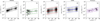 |
Fig. 1 Density maps of values of standard error, σ(υɡ), as function of geocentric speed, υɡ, for databases used in this study (see Table 1). In all panels, the solid coloured line plots the result of a linear fit in the linear-log space, and the dashed coloured lines mark the corresponding prediction band at a 68% confidence level. |
2.2 Precision and accuracy of meteor data
At first, the precision level of the data acquired and processed by meteor and fireball networks can be assessed by analysing the uncertainties provided in the corresponding catalogue. In particular, in this section we consider those of the geocentric quantities (i.e. the geocentric speed of a meteor, υɡ, and the angular elongation of the meteor geocentric radiant from the Earth’s apex, ϵɡ) that we use to demonstrate our approach (see Sect. 3).
As an example, we now consider the uncertainties given for the geocentric speed, υɡ Figure 1 presents, as a function of υɡ, the density maps of the values of the standard error associated with it, σ(υɡ), as reported by the networks considered in this study (see Sect. 2.1). Regardless of the specific database, it is possible to observe that the magnitude of σ(υɡ) increases as υɡ increases, which is an already well-known behaviour (e.g. Vida et al. 2020b). In order to highlight this increase, we evaluated a linear fit (in a linear-log space) of σ(υɡ) against υɡ, plotted as a coloured solid line in each panel, as well as its prediction band at a 68% confidence level, whose extrema are plotted as dashed coloured lines. This increase can be attributed to different factors. Generally speaking, a faster meteor implies a shorter phenomenon, meaning a shorter observation time span and a lower number of points with which to triangulate the trajectory. Furthermore, in the case of video observations, the point spread function (PSF) of the meteor image on a single frame becomes more elongated as the apparent speed increases, thus implying a higher level of uncertainty in the determination of the position of the meteor in each frame. The relatively large spread of σ(υɡ) around the central lines is due to the fact that many other factors influence the achievable precision of each observation. Among said factors, the most obvious ones are the magnitude of the meteor with respect to the sensitivity of the instrument and the distance of the meteor from the observers.
At present, the highest precision claimed for speed measurements is of the order of 10 m s−1 for the fireballs observed by EFN, as shown in Fig. 1b. This plot shows that such a small error magnitude is only achieved in the best-case scenario; that is, in the best observational conditions. The average precision level is of the order of 100 m s−1, without ever exceeding 1 km s−1 even when considering the highest geocentric speed in the database. A few other meteor networks, such as the video meteor observations of the Ondřejov observatory and GMN, report speed measurements with a similar – yet slightly lower – precision level of the order of 100 m s−1.
Compared to the above-mentioned meteor and fireball networks, both FRIPON and CAMS report a lower nominal precision level. In both these databases, the average value of σ(υɡ) for lower modules of geocentric speed is greater than 100 m s−1. Furthermore, Fig. 1 clearly shows a difference between FRIPON and all the other databases taken into consideration, the difference being that the average value of σ(υɡ) increases significantly more steeply as a function of υɡ.
Although there are many other meteor networks and databases that report comparable precision and accuracy levels, their data are not yet openly available. For instance, the Canadian Automated Meteor Observatory6 (CAMO; Vida et al. 2021a) reports speed measurements with an accuracy of 100 m s−1. Similarly, the Spanish Meteor Network7 (SPMN; Madiedo & Trigo-Rodríguez 2008; Peña-Asensio et al. 2021) and the Desert Fireball Network8 (DFN; Sansom et al. 2019; Devillepoix et al. 2019) report high-accuracy orbits of fireballs with a speed error of less than 1 km s−1. On the other hand, many other national and multinational networks make their data openly available, but without providing any uncertainties on the parameters of their databases, even though they may be able to provide meteor observation data with comparable precision and accuracy levels. This is the case of the Japanese catalogue9 (SonotaCo 2009, 2016) and the European viDeo Meteor Observation Network database10 (EDMONd; Kornoš et al. 2014).
Instead, an a priori assessment of the accuracy in the results of the meteor observations carried out by these different networks is more complicated. Less accurate results might come from simplifications and assumptions that are usually adopted within the data reduction pipeline. Here are a few examples: (1) potential biases in the astrometric reduction of the observations in case of heavily distorted all-sky images (Borovička et al. 1995; Jeanne et al. 2019; Barghini et al. 2019); (2) the straight-line hypothesis in the triangulation of the meteor trajectory (Borovička 1990; Gural 2012; Sansom et al. 2019; Vida et al. 2020b; Spurný et al. 2020); (3) the assumptions about the drag coefficient, its constant value (Khanukaeva 2004), and the atmospheric density profile (Lyytinen & Gritsevich 2016) when evaluating the deceleration of the meteoroid during its bright flight; (4) the assumption of a two-body problem (ignoring the gravitational effect of other major bodies of the Solar System) when determining the pre-atmospheric orbit of the meteoroid (Clark & Wiegert 2011; Dmitriev et al. 2015; Jansen-Sturgeon et al. 2019). The relative accuracy between the observations of different meteor and fireball networks can be evaluated when two or more networks detect the same event. However, in this case data are usually combined in a single analysis, rather than being independently compared, in order to provide a more comprehensive picture of that specific phenomenon (e.g. Jenniskens et al. 2019, 2020; McMullan et al. 2024). In this regard, simulation studies might provide further insights and allow for a direct assessment of the relative and absolute accuracy of such observations (Shober et al. 2023).
Apart from the geocentric speed, υɡ, the other geocentric quantity used in our approach is the elongation, ϵɡ, of the meteor geocentric radiant with respect to the Earth’s apex. This quantity is not usually explicitly reported in the databases of meteor observations, but it can easily be computed if given the geocentric radiant coordinates, (αɡ, δɡ), and the date and time of observation (see Sect. 3). Our inspection of the standard errors of the radiant elongation, σ(ϵɡ), has not highlighted any significant variation of its magnitude as a function of either υɡ or ϵɡ. Nevertheless, the precision in the determination of ϵɡ rather depends on the geometry of the observations and the number of cameras involved in the detection, as is the case in most of the databases considered in this study (not shown). In every case, both of the above-mentioned geocentric parameters of a meteor, (υɡ, ϵɡ), strongly influence the determination of the resulting heliocentric speed of the meteoroid and, consequently, the determination of its orbit.
3 Methods
The optical observation of meteors from different observation sites makes it possible, thanks to the triangulation principle, to measure the initial velocity of the meteoroid at the top of the atmosphere. From the triangulation results, it is possible to infer the pre-atmospheric speed, υ∞, accounting for the atmospheric drag if the latter is significant before the visible flight of the meteor. Therefore, three-dimensional orientation of the atmospheric trajectory defines the pre-atmospheric velocity vector,  , which is then corrected for the zenith attraction effect due to the Earth’s gravity and from which we can derive the geocentric velocity vector,
  (Dubyago 1961). Finally, the heliocentric velocity vector,
  , can be given as the vectorial sum of the geocentric velocity and the Earth’s revolution velocity,
  . The module of the heliocentric velocity vector is already diagnostic of the nature of the meteoroid orbit, since it directly refers to the value of the semi-major axis, a, of its orbit in the hypothesis of the two-body problem:
 (1)
(1)
where µ = GMS is the heliocentric gravitational parameter and R0 is the Earth’s distance from the Sun. The parabolic limit is then given by the condition 1/a → 0 that can be written as υp = 42.1 km s−1 and varies approximately between 41.8 and 42.5 km s−1, since R0 also varies from 0.983 to 1.017 au along the Earth’s orbit. It is therefore clear that the extension of the confidence region of υh with respect to υp will determine the significance level with which the orbit can be considered hyperbolic.
In order to do so, the analysis of measurement errors is of utmost importance. Since the uncertainty of υh originates both from the error of the module and from that of the direction of υɡ in the Earth-centred inertial (ECI) coordinates, Hajduková et al. (2019) proposed using a graph based on these geocentric quantities to analyse hyperbolic meteors. The graph illustrates the direct impact of meteor measurement errors on the resulting meteoroid orbits and is based on the original work of Kresák & Kresáková (1976). This result is achieved considering the square module of the heliocentric velocity vector as follows:
 (2)
(2)
where ϵɡ is the angular elongation of the geocentric radiant from the Earth’s apex.
Therefore, the (υɡ, ϵɡ) diagram can also be used as a tool for the initial assessment of the accuracy of error estimation. To facilitate its use for this purpose, we suggest naming it the Kresáks’ diagram, after the authors of the original paper, L’ubor Kresák and Margita Kresáková.
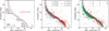 |
Fig. 2 Visualisation of the Kresáks’ diagram, showing relationship between geocentric meteor parameters and resulting heliocentric meteoroid orbits. The different dashed black lines represent orbits with varying values of semi-major axes (see legend of panel b), and the red lines plot the parabolic limit. Panel a displays the position on the Kresáks’ diagram of simplified areas corresponding to the orbit type of each event shown in the graph. Panels b and c demonstrate the approach using older photographic meteors reported in eight IAU MDC catalogues. Panel b represents all photographic catalogues together, with the parabolic limit dividing the diagram into two regions, which are those of meteoroids on elliptical orbits (grey crosses) and hyperbolic orbits (red crosses), showing a continuous spread between the two (Hajduková et al. 2019). Panel c displays the photographic orbits colour-coded according to their respective catalogues and reflecting their data quality. Hereafter, the selected catalogues and their labels in panels b and c are as follows: C – 103 orbits, Ceplecha’s small camera; D – 636 orbits, Dushanbe stations; E – 180 orbits, European Network; J – 413 orbits, Harvard Super Schmidt camera; K – 206 orbits, Kiev stations; O – 459 orbits, Odessa stations; R – 32 orbits, Spanish meteor society; and W – 166 orbits, Harvard small cameras. |
3.1 The Kresáks’ diagram
Figure 2 shows the relationship (υɡ, ϵɡ), which effectively displays various dynamical populations of meteoroids and/or sources of meteors (as described, e.g., by Jacchia & Whipple 1961). The meteor data shown in the plot are selected from version 2023-II of the IAU MDC photographic catalogues (Neslušan et al. 2014). Due to the correlation between υɡ and ϵɡ, most orbits fall within a relatively narrow region on the diagram. In particular, this correlation shows that meteoroids crossing the Earth’s orbit exhibit a wide range of geocentric speed (11–72 km s−1 for local meteoroids), but a narrow range of heliocentric speed (about 36–42 km s−1).
The theoretical curves in Fig. 2 are constructed for various chosen values of the semi-major axis, a. The red line represents the parabolic limit, marking the boundary beyond which hyperbolic orbits are found. The orbits of Solar System meteoroids are confined to the portion of the graph on the left side of the red curve.
Low values of the angular elongation correspond to fast meteoroids that meet the Earth head-on, while high values of elongation correspond to relatively slow meteoroids that catch up with the Earth. The upper left area (above ϵɡ > 60°) of the diagram corresponds to orbits associated with short-period comets, while the lower right region corresponds to orbits related to long-period comets. Asteroidal orbits with perihelion inside the Earth’s orbit are located in the lower left area, with a moderate concentration near ϵɡ ~ 90°.
The sparse area around υɡ ~ 50 km s−1 and ϵɡ ~ 50° corresponds to nearly perpendicular crossings of orbits, which necessitate an orbit with either a high inclination11 or a low perihelion distance. These types of orbits are difficult to observe, which contributes to the bimodal speed distribution related to the Earth, with a clear minimum occurring between 45 and 55 km s−1 (e.g. Wiegert et al. 2009). We recall that the bimodality of the geocentric speed distribution arises from various factors. One of them is the influence of the apex and antapex effects when observing meteors from the Earth (Jenniskens 2006), which manifest as the diurnal variation in meteor frequencies and the AM/PM asymmetry in meteorite fall times. Another major factor is the distribution of meteoroid orbits in space (McKinley 1961; Millman & McKinley 1963), which involves the concentration of short-period orbits in the ecliptic plane and the random distribution of the planes of long-period orbits. Additionally, the υɡ-distribution is influenced by the observation technique employed and the method used for velocity determination (Brown et al. 2004).
3.2 Beyond the parabolic limit
Figure 2 highlights a clear spread of meteoroids beyond the parabolic limit. We deliberately chose a database of meteors from photographic observations that, despite being old, has always been considered relatively accurate. The photographic IAU MDC database (Neslušan et al. 2014) is compiled from eighteen different catalogues and does not provide uncertainties for meteor parameters. Said catalogues contain data obtained with various equipment and software, resulting in various levels of accuracy (Hajdukova 1994). Consequently, the proportion of hyperbolic orbits varies considerably among the individual catalogues, each one identified by a different colour in Fig. 2c. For greater transparency, it is important to point out that, out of the 18 original catalogues, we plot eight, which contain a total of 42 partial catalogues. This selection was created taking into account the level of accuracy of the individual catalogues, as discussed by Hajdukova (1994).
The lower quality catalogues (D, K, and O) present a large fraction of hyperbolic orbits (18.40%, 30.10%, and 30.07% of the total number of orbits, respectively) with high heliocentric excess speeds (up to 31.2 km s−1 above the parabolic limit). On the other hand, the higher accuracy catalogues (C, E, J, R, and W) present a lower fraction of hyperbolic orbits (17.48%, 11.67%, 2.18%, 0%, and 12.05% of the total number of orbits, respectively) with very gentle excess speeds (up to 2.8 km s−1 above the parabolic limit). This difference confirms the already known dependence of data quality on the number of hyperbolic orbits in the data.
It is important to highlight that the observed spread of orbits beyond the parabolic limit is continuous and most abundant on the parabolic limit itself and in the region of high geocentric speeds. This does not reflect the expected speed distribution for a real population of interstellar meteors, as also discussed in Appendix A.2.
Another interesting aspect that can be observed in the Kresáks’ diagram is the significant accumulation of hyperbolic events corresponding to known meteor showers. Indeed, these meteor showers are usually very close to the parabolic limit, having long-period comet-like orbits with a high semi-major axis. Therefore, it is clear that even a very small measurement error on either υɡ or ϵɡ may cause one point on the diagram to be artificially moved beyond the parabolic limit and to be classified as interstellar.
Based on simulations of Perseid-like orbits affected by measurement errors of varying magnitude, Hajduková & Kornoš (2020) suggested that a precision and accuracy level of ~0.1 km s−1 for the pre-atmospheric speed and of ~0.1º for the radiant position is needed in order to confidently identify interstellar meteors within the data. A simulation of a lower accuracy level of 1 km s−1 and 1º of the above-mentioned quantities resulted in a significant proportion of orbits (one third of the simulated sample) being determined as hyperbolic. Therefore, identifying individual interstellar meteors in data of such low accuracy is not possible. Indeed, any potential interstellar particles remain unconfirmed within the margins of errors.
3.3 Estimating error bars
When displaying the geocentric quantities, (υɡ, ϵɡ), and observing the resulting orbits within the same plot (Fig. 2), it becomes possible to estimate the limits of the uncertainties of said quantities (whether provided or not), which significantly influence the orbital elements and, consequently, the orbit type of the meteoroid. In other words, the resolution of the Kresáks’ diagram enables the estimation of the accuracy required to distinguish between different orbit types.
However, the required accuracy varies depending on the resolution in different areas of the diagram. Distinguishing between orbits with different semi-major axes is most challenging near the parabolic limit due to the resolution within this area of the diagram. The highest accuracy is required at this limit and, in particular, around larger geocentric speeds, such as that of the Perseid stream meteoroids. For observed meteors that fall within this region, uncertainties of the order of 1 km s−1 in speed and 1° in radiant position, as commonly reported in multiple databases, may lead to misclassification, thus affecting not only the dynamical characterisation of the particle and its potential origin, but also the subsequent interpretations of its structure and composition.
The diagram allows for the estimation of the uncertainties in speed and radiant position that may have geometrically shifted the event above the parabolic limit. The term ‘geometrically’ emphasises that this shift pertains to the nominal value of υh, without any specification regarding its confidence region on the plot thus far. Indeed, the extensions of errors in υɡ and ϵɡ could still render the event compatible with the profile of a closed orbital configuration, placing it on the left of the parabolic limit.
This application of the Kresáks’ diagram was first shown by Hajduková et al. (2024) in the case of the CNEOS fire-ball database. In short, the method consists of varying the uncertainties assigned to the velocity vector components and of evaluating, for each event under consideration, whether or not the 3σ confidence region on the Kresáks’ diagram intersects the area to the left of the parabolic limit, thus rendering it compatible with a closed orbit configuration. With particular reference to the population of hyperbolic meteors, said study showed that a 1σ standard error of 6.4 km s−1 on the geocentric speed and 8° on the radiant elongation is enough to reject all CNEOS interstellar candidates at a 99.9% confidence level. Such an order of magnitude for the standard error on both parameters was also supported by Hajduková et al. (2024) through a statistical analysis of the complete CNEOS database and a simulation of the uncertainties of satellite measurements according to image resolution.
Conversely, there is currently an increasing number of databases that provide uncertainties demonstrating sufficient accuracy to confidently identify hyperbolic orbits. In such data, a misclassification of orbits occurs when uncertainties are underestimated, or better, because they reflect the precision of the parameters rather than their accuracy. Hence, it may occur that reported high-precision orbits do not represent high-accuracy orbits. Indeed, this is a growing problem.
3.4 Confidence regions on the Kresáks’ diagram
If a given meteor database provides an estimation of parameter uncertainties, the Kresáks’ diagram can be used to test the significance of a single candidate to actually be hyperbolic, thus suggesting or disputing its interstellar nature.
Figure 3 visualises the confidence region with a zoomedin view of the Kresáks’ diagram for two examples of artificial meteor. In both cases, we assumed predefined values for the pre-atmospheric speed, υ∞ = (65.7 ± 0.4) km s−1, and for the pre-atmospheric radiant position, α = (153 ± 1)° and δ = (5 ± 1)°. The uncertainties of these parameters are assumed to represent standard errors according to a Gaussian distribution. By replicating the data-reduction procedures outlined in the introduction of Sect. 3, and according to the linearised propagation of standard errors, we derived the following geocentric quantities of the artificial meteors and their standard errors: υɡ = (54.4 ± 0.4) km s−1 and ϵɡ = (37 ± 1)°. Such errors can be visualised in both panels as cyan error bars, and the blue lines draw the boundaries of the 1σ (68.2%), 2σ (95.4%) and 3σ (99.7%) confidence regions.
At the chosen significance level, the key point of the analysis is to evaluate the extension of these confidence regions with respect to the parabolic limit, plotted in Fig. 3 as the red thick line. From a numerical point of view, it is possible to determine whether or not any intersection points exist between the selected confidence region boundary and the parabolic limit curve. At each one of the significance levels considered, panel a shows that the confidence region is always on the right side of the parabolic limit without intersecting it; hence, the meteor candidate can be considered significantly hyperbolic. This is not true for the case of panel b, where the 3σ ellipse extends to the left of the parabolic limit, meaning that the corresponding orbit cannot be considered hyperbolic at a 0.14% significance level (given that the hypothesis test is actually one-sided).
At this point, it is important to clarify what is the difference between Figs. 3a and b, since both simulations started from the same nominal values of speed and radiant position and their given standard uncertainties are the same. The subtle difference in question regards the introduction of non-diagonal values of the covariance matrix assumed alongside the error propagation. In particular, panel a assumes a correlation between υ∞ and α of +0.3, whereas panel b assumes a correlation of −0.3 (while all other non-diagonal covariance terms are assumed to be null). This small difference modifies the orientation of the confidence region on the Kresáks’ diagram. As we just commented, this subtle change drastically alters the conclusion that can be drawn regarding the nature of the event under analysis. Non-diagonal covariance terms are most often neglected and not reported in meteor databases. Instead, this example clearly shows how crucial all information on the covariance matrix is in our analysis.
Furthermore, the underlying distribution of points plotted in both panels of Fig. 3 reports the result of a Monte Carlo boot-strap error propagation. An ensemble of 300 replicas of υ∞,i, αi, and δi was generated, according to a normal Gaussian distribution centred on the assumed nominal values and standard errors, and then processed through the whole pipeline ultimately producing the output ensemble of (υɡ,i, ϵɡ,i) that is plotted in the figure. The result of this process helps to visualise and verify the appropriateness of the linearisation assumption done through standard error propagation. In this case, the confidence ellipses and the distribution of points nicely match. With errors of larger magnitude for the speed and/or the radiant position, it is always important to perform such a verification, because the shape of the actual confidence regions might be misrepresented by an ellipsoid.
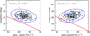 |
Fig. 3 Visualisation of confidence regions for geocentric quantities on the Kresáks’ diagram for two simulated meteors. In both panels, the parameters of the observed meteor were generated as υ∞ = (65.7 ± 0.4) km s−1, α = (153 ± 1)°, and δ = (5 ± 1)°. The corresponding nominal values and standard errors for υɡ and ϵɡ are reported as cyan error bars. The blue ellipses, from inner to outer, show the boundaries of the 1σ, 2σ, and 3σ confidence regions, and the red line plots the parabolic limit. The black dots represent the result of a bootstrap Monte Carlo error propagation for an ensemble of 300 repetitions. The simulation included a covariance matrix element for (υ∞, α) of +0.3 for panel a and of −0.3 for panel b. |
4 Results and discussion
In our analysis, we applied the Kresáks’ diagram to the databases of several video meteor networks. Among these, we also included two quite recent databases, FRIPON and GMN, and meteor observation data from the CAMS database and the Czech video catalogue. For comparison, we also included a population of much larger meteoroids and plotted fireballs from the EFN and the CNEOS catalogues.
The diagrams are shown in Fig. 4 as density plots, because of the large difference in the number of orbits among all the selected catalogues. In all the datasets, it is possible to observe a tail above the parabolic limit, especially in the range υɡ > 50 km s−1 where it is most challenging to obtain the required accuracy for distinguishing between different types of orbits. The percentage of geometrically hyperbolic events is similar in the FRIPON and CAMS databases (around 12%) and slightly lower in the GMN catalogue (about 8%; see Table 1). The Czech catalogues of video meteor data present a lower fraction of hyperbolic orbits (about 2%). This is most likely due to the precise and manually performed meteor measurements compared to the automatic measurements and data-reduction pipelines used in the other databases.
It is important to recognise that we are comparing data from networks that provide unfiltered datasets, such as CAMS, with others that process and select data, such as GMN. This is evident from the continuous spread (Fig. 4f) when compared to the cutoff of data (Fig. 4b) beyond the parabolic limit at certain levels on the Kresáks’ diagram.
Furthermore, it is important to acknowledge the differences caused by different observations and their sensitivity to various meteor populations. Indeed, meteor databases often focus on cometary meteor showers, most of which have long-period and retrograde orbits (positioned in the bottom part of the Kresáks’ diagram when ϵɡ < 50°). Such orbits are more likely to exceed the parabolic limit due to measurement errors, even if they are just very small ones. Indeed, distinguishing between orbits with different semi-major axes is most challenging in the lower area of the Kresáks’ diagram because of its resolution. The problem is further amplified by the fact that higher geocentric speeds usually cause larger errors (see Fig. 1). In contrast, the fireball databases mainly contain prograde asteroidal orbits with lower geocentric speeds (positioned higher on the Kresáks’ diagram when ϵɡ > 50°).
As expected, the fraction of hyperbolic orbits is similarly low in both the EFN and the CNEOS fireball databases. However, the spread of meteors beyond the parabolic limit and the magnitudes of their hyperbolic excesses are not similar. The EFN hyperbolic meteors only exceed the parabolic limit in the region of the Kresáks’ diagram where the highest precision level is required, with eccentricities only slightly above 1. In contrast, the hyperbolic events in the CNEOS catalogue extend beyond the limit across the entire speed range and reach eccentricities of up to 2.4.
The hyperbolic orbits in the CNEOS catalogue were thoroughly examined by Hajduková et al. (2024). The study concluded that all of the CNEOS geometrically hyperbolic meteors did not exhibit interstellar characteristics and that the apparent hyperbolicity of their orbits was probably caused by measurement errors. These conclusions were supported by significant deviations in one velocity component and by a dedicated simulation that revealed a radiant dispersion of up to 15° (see also Sect. 3.3).
Despite the objective differences between the data compared in Fig. 4, the fraction of hyperbolic events that they present provides an independent first estimate of the quality of the databases. More detailed information is then provided by the abundance of hyperbolic events that survived the 3σ filtering, which are marked with red crosses in all the panels of Fig. 4, except for the panel representing the CNEOS catalogue, as it does not report uncertainties. The 3σ residuals provide insight not only into the accuracy of the parameters, but also into their uncertainties. Indeed, in the next sections we discuss how, when taking into consideration these uncertainties on the Kresáks’ diagram, it is possible to identify significant differences among the chosen datasets.
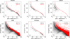 |
Fig. 4 Density representation of the Kresáks’ diagram for databases of (a) FRIPON, (b) GMN, (c) EFN, (d) Ondřejov, (e) CNEOS, and (f) CAMS, given in logarithmic greyscale. The red curve plots the parabolic limit, and the red crosses represent hyperbolic events that overpass such limit with a p value lower than 0.14% (3σ). Each panel also displays the percentage of hyperbolic (black) and 3σ hyperbolic (red) events. |
4.1 Significance of the hyperbolic orbits
Understanding how the inclusion of measurement errors in this analysis affects its results is crucial. To do so, we progressively varied the confidence level – that is, the number of standard deviations, Nσ, used to define the confidence region on the Kresáks’ diagram (see Sect. 3.4) – and we evaluated the fraction of events in each database that survives this filtering process. This is the most commonly used approach within the community of meteor astronomers. In order to define the confidence interval for each corresponding confidence level, this approach relies on a null hypothesis test based on the assumption of a Gaussian statistical model to interpret the database parameters of a meteor and their uncertainties as expected values and standard deviations of the distribution of the measured values. Similarly, we computed and analysed the fraction of shower-related events within the hyperbolic subset for each confidence level, according to the arguments presented in Appendix A.3.
The results of this simple yet enlightening analysis are reported in Fig. 5. Panel a plots the trend of the hyperbolic fraction, as a function of Nσ, for the three databases under examination. This trend is ultimately linked to the distribution of events above the parabolic limit, although the distance (i.e. the hyperbolic excess) of each event is weighted according to the extension of its confidence region. In all cases, the percentage of hyperbolic events drops as the value of Nσ increases. However, this decay is much steeper for FRIPON with respect to the GMN and CAMS, which are both characterised by a different very similar trend. Taking Nσ = 3 as a reference (i.e. one-sided 99.86% confidence level), the percentage of hyperbolic events is as low as 0.26% (18 events) for FRIPON and 0.24% (two events) for Czech video meteors catalogue, compared to 1.36% and 2.90% for GMN and CAMS, respectively.
The 3σ filtering for the hyperbolic cases of EFN was investigated by the authors of this catalogue (Borovicka et al. 2022b,a). The sample of 824 fireballs contained 18 hyperbolic orbits and, out of those, only two remained hyperbolic within the 3σ uncertainty interval (the two red crosses in Fig. 4e). The speeds of the two events were measured with a precision of 0.1 km s−1 and 0.2 km s−1, respectively, and their radiant positions were determined with a precision of less than 0.1°. Since their hyper-bolic excesses were very low (i.e. the eccentricity of their orbits did not exceed 1.05), Borovička et al. (2022a) concluded that it is highly probable that these two orbits became hyperbolic due to processes within the Solar System, thus confirming the non-detection of interstellar meteoroids in the centimetre-to-decimetre size range.
This specific example from the EFN data highlights how, in general, the 3σ filtering alone cannot reveal whether the residual events can be effectively addressed as interstellar meteoroid candidates or not. Obviously, we cannot exclude the presence of a single interstellar particle among them; however, this cannot be indisputably proven. On the other hand, it would not be reasonable to simply state that those events are not a priori hyperbolic, because, among other reasons, they survived a quite selective 3σ filtering. However, the abundance of such events on the Kresáks’ diagram (red crosses in Fig. 4) suggests that we cannot classify them as candidates for interstellar particles, unless they are found in the most accurate databases, due to the following two main factors: the non-peaked distribution of their heliocentric speed, which continuously decreases after the parabolic boundary, and the abundance of shower meteoroids among hyperbolic events (see Appendix A).
An example of the latter can be easily observed in Fig. 5b, which plots the percentage of shower-related meteors within the hyperbolic subsets of the considered databases, as a function of Nσ. In the case of the FRIPON database, shower-related meteors within the hyperbolic subset are efficiently filtered as Nσ increases, even in spite of the fact that FRIPON shows the higher fraction of geometrically hyperbolic shower meteors among the three databases in question (see Table 1). At Nσ = 5.5, all shower events are removed from the hyperbolic subset. On the other hand, this fraction is quite steady as a function of Nσ in the case of the GMN and the CAMS databases, with a relative drop of only 5–10%.
This represents clear evidence that the filtering process according to the measurement errors is not effective, and that the events that survive this selection still do not represent real candidates of interstellar meteors. On the same topic, it is also quite interesting to notice that the fraction of hyperbolic events at Nσ = 3 for the FRIPON, EFN, and Ondřejov data is of the same order as the percentage of events that would be expected to lay outside the one-sided 3σ confidence interval; that is, 0.14%.
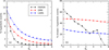 |
Fig. 5 Significance of hyperbolic orbits in the FRIPON, GMN and CAMS meteor databases. Panel a shows the fraction of hyperbolic events as a function of the confidence level expressed as Nσ, which represents the number of standard deviations used to define the confidence interval in the Kresáks’ diagram. The coloured curves represent the fitting of Eq. (3) over the results of each database. Panel b displays the fraction of meteors associated with known meteor showers belonging to the hyperbolic subset as a function of Nσ. |
4.2 Underestimation of meteor data uncertainties
In the previous section, we highlighted how the process of filtering hyperbolic events, according to the considered measurement errors, does not appear to be effective. We can now take one step further and interpret the shape of the relative drop of the hyper-bolic fraction as a function of Nσ (see Fig. 5b). If we hypothesise that any of the events in these datasets can be significantly identified as hyperbolic, we can expect their distribution above the parabolic limit to be given in the form of
![Mathematical equation: $f\left( {{N_\sigma }} \right) = {f_0} + {{1 - {f_0}} \over 2}{\rm{erfc}}\left[ {{1 \over {\sqrt 2 }}\left( {{{{N_\sigma }} \over R} + B} \right)} \right].$](/articles/aa/full_html/2025/09/aa54274-25/aa54274-25-eq7.png) (3)
(3)
This equation is valid if the measurement errors can be assumed to represent the width of a Gaussian distribution. Within Eq. (3), ƒ0 represents the actual fraction of hyperbolic events12, while R can be interpreted as an estimator of the goodness of the error determination within the dataset. In fact, R = 1 corresponds to the instance in which the fraction of hyperbolic events drops beyond the parabolic limit as the cumulative function of a normal distribution does. On the other hand, R > 1 highlights how this drop is slower and may suggest that the measurement errors are being underestimated (or overestimated if R < 1). Finally, B is related to the fraction of geometrically hyperbolic events (at Nσ = 0) and, as already mentioned, it can vary among different datasets for various reasons. The results of the fitting of Eq. (3) over the data of the FRIPON, GMN, and CAMS catalogues are plotted as the coloured curves in Fig. 5a. We determined R = 1.19 ± 0.05 for FRIPON and R = 3.10 ± 0.02 for both GMN and CAMS. This evidence further supports our preliminary conclusions, indicating that the FRIPON database provides a good error estimation. On the other hand, this model suggests that the magnitude of errors given in the GMN and CAMS databases is significantly underestimated.
The same analysis was performed for the Ondřejov and EFN data. Nevertheless, the results of this analysis are influenced by the very limited statistics on the geometrically hyperbolic events of these two databases. The optimisation of Eq. (3) highlighted a value of R = 1.8 ± 0.9 for the Ondrejov data and of R = 4 ± 3 for the EFN data. In both cases, R is compatible with 1, but it is determined with a confidence interval that is too large to provide a diagnostic conclusion, which might be reached in the future with a larger sample size. In any case, the very low percentage of hyperbolic orbits in these two databases suggests that the uncertainty estimation for such data can be considered reliable.
Complementarily to what is presented in Fig. 1, the precision of the data reported by the authors can be visualised by directly plotting the distribution of the provided uncertainties, as illustrated in Fig. 6. The filled histograms represent the error distribution provided for the data, while the superimposed and not filled histograms present the specific distribution of uncertainties of the hyperbolic dataset (at a 3σ confidence level). The distributions of the radiant uncertainties are quite similar, but the speed uncertainties differ. FRIPON has a modal uncertainty of 0.3 km s−1, whereas GMN presents a typical error of 0.1 km s−1 consistent with what is shown in Fig. 6e. For comparison, the modal speed uncertainty of the CAMS database stands in between these values, at about 0.2 km s−1. Another difference between the datasets is shown by the hyper-bolic error distributions. In particular, the selection of data in the FRIPON catalogue appears to be non-random. Assuming that the hyperbolic events do not represent an interstellar population, as suggested above, the uncertainties of these events should reflect the largest inaccuracies; they should therefore be shifted to larger values compared to all other events in Fig. 6. However, this is not the case with the GMN and CAMS data, suggesting that the errors provided by these two databases are underestimated, to the extent that they do not reflect the actual measurement uncertainty. Similarly, it is also possible to notice that the distribution of σ(ϵɡ) for the hyperbolic subsets of GMN and CAMS is skewed towards lower values, instead of preferring larger uncertainties, as is the case with the FRIPON data.
Going one step further, we can also test the hypothesis of a possible underestimation of the uncertainties provided in meteor databases. In particular, the same concept displayed in Fig. 5 can be implemented in order to visualise the median value of these uncertainties as a function of Nσ. The result of this analysis is reported in Fig. 7 for both σ(υɡ) and σ(ϵɡ). According to what is discussed above for Fig. 6, it would be possible to expect the uncertainties to become larger as Nσ increases, thus moving farther from the parabolic limit. However, this is again not true in the case of GMN and CAMS; indeed, both σ(υɡ) and σ(ϵɡ) monotonically decrease as a function of Nσ. This means that, even though they could at first be regarded as the best candidates for the detection of interstellar particles in the Earth’s atmosphere, the hyperbolic events that are farther away from the parabolic limit are actually selected in this way because the uncertainties associated with their parameters are systematically lower than they are for other events. Furthermore, once again, the behaviour of the FRIPON dataset is the opposite, meaning that uncertainties generally increase as a function of Nσ; therefore, events that are farther away from the parabolic limit, probably as a result of mismeasurement or biased assumptions, are consistently associated with larger errors in the FRIPON database.
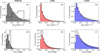 |
Fig. 6 Distributions of uncertainties in geocentric speed, σ(υɡ), (panels a, c, and e) and in radiant elongation, σ(ϵɡ), (panels b, d, and f) as reported in the respective databases (i.e. FRIPON, GMN, and CAMS, the three largest ones considered in this study). Distributions are shown separately for all events (filled histograms) and for hyperbolic events that survived the 3σ filtering (empty histograms). |
5 Conclusions
In this paper, we present a tool for the initial assessment of the actual accuracy of meteor data (in particular, the geocentric quantities υɡ and ϵɡ) and propose calling it the Kresáks’ diagram, after the authors of the paper in which the concept was first introduced (Kresák & Kresáková 1976). The diagram simultaneously displays the geocentric parameters of a meteor and the resulting heliocentric orbit of the meteoroid prior to its encounter with the Earth. The resolution of the diagram allows for the estimation of the required accuracy of the geocentric speed and radiant needed to unambiguously determine the type of orbit of each meteor. The accuracy required depends on the specific area of the diagram being taken into consideration, as the resolution varies across it.
The most challenging area of the diagram is near the parabolic limit, especially when dealing with large geocentric speeds. Beyond this region, it may be possible, using precisely determined orbits, to identify a priori samples or individual cases of interstellar particles, but only after having excluded all hyperbolic orbits resulting from processes within the Solar System (Wiegert 2014). Among the databases used in our study, only the EFN database (Spurný et al. 2017; Borovicrka et al. 2022b) meets the accuracy requirements; this is because the uncertainties cover all hyperbolic cases, with the exception of two residual meteors with very minor hyperbolic excesses. The other Czech video meteor data, provided by the Ondřejov observatory (Koten et al. 2003) and partly manually reduced, approach the required accuracy level as well. Since collisions with meteoroids of interstellar origin are highly unlikely (though not impossible), the limitation of these two databases in identifying them lies in the small number of detectable events. However, high-accuracy orbits are at the basis of a wide range of research possibilities.
The other meteor databases considered in this study deploy fully automated reduction procedures, which show a large number and a continuous spread of residual hyperbolic meteors, thus demonstrating that the filtering process – based on their reported measurement errors and on a commonly used null hypothesis test – is not effective. Therefore, we developed an estimator of the goodness of error determination in order to evaluate the slope of the decrease of the hyperbolic fraction of the data with increasing confidence level. This estimator points out underestimated errors when R > 1, or overestimated errors when R < 1, with respect to the cumulative function of a normal distribution. It must be noted that R, by definition, specifically refers to the population of meteors close to the parabolic limit. For this reason, it is diagnostic of a possible underestimation or overestimation of database uncertainties only in this region of the Kresáks’ diagram. Therefore, this estimator can be used to test the appropriateness of the error estimation and treatment within a meteor observation database with the purpose of identifying potential candidates of interstellar meteors.
When applied to the databases, this estimator yielded R = 1.19 ± 0.05 for FRIPON and R = 3.10 ± 0.02 for both GMN and CAMS. Therefore, according to our approach, we can conclude that the uncertainties of most of the databases taken into consideration appear to be underestimated, at least for meteors close to the parabolic limit. This is true not only for the older sample of CAMS data (Jenniskens et al. 2011, 2016), reduced by a well-established software (Gural 2012), but also for the most recent GMN data (Vida et al. 2021b), analysed via a more sophisticated reduction pipeline (Roggemans et al. 2024) and including a novel trajectory-estimation method developed by Vida et al. (2020a,b). The precision of the GMN data is higher; nevertheless, the uncertainties determined appear not to encompass the possible range within which the actual value of the parameters lies. Vice versa, the FRIPON data (Jeanne et al. 2019; Colas et al. 2020) report a lower level of precision, but the distribution of their uncertainties exhibits a behaviour that more closely reflects the actual data accuracy.
As a matter of fact, the pipeline developed for the reduction of the FRIPON meteor data pays particular attention to providing “[…] an estimate of internal and external errors as realistic as possible” (Jeanne et al. 2019). Indeed, the authors developed a novel statistical method to take into account the possible systematics affecting the observation and measurement of a meteor by each camera; that is, a least-squares regression on a modified sum of residuals. In this method, they assigned a particular weight to the data considered in the triangulation process (Ceplecha 1987; Borovicka 1990) on the basis of the astrometrical measurement noise, the number of images, and the accuracy of its calibration as evaluated from the results of the astrometric calibration process. In this regard, a common misconception in the reduction of meteor and fireball network data might be to assume that every measurement (i.e. every frame) of each observation of the same meteor always represents a separate degree of freedom when combining data from different cameras within the meteor triangulation process. The issue of this possible misconception was first highlighted by Jeanne et al. (2019) for the FRIPON data and later by Barghini (2023) for the data of the PRISMA Italian fireball network, partner of the FRIPON international consortium.
In general, while it cannot be ruled out, the presence in such data of a single truly hyperbolic event caused by an interstellar particle cannot be conclusively identified either. There are no additional criteria, beyond hyperbolic speed, to distinguish such a particle from an interplanetary one, as the meteor phenomenon it causes in the atmosphere is the same. Only its characteristics relative to the Sun, rather than to the Earth, can be differentiated. Paradoxically, according to the analysis presented, the likelihood of detecting an interstellar particle using optical techniques is higher for slow meteoroids relative to the Earth than it is for fast ones approaching the Earth head-on.
The results of this article demonstrate that determining the uncertainties requires improvements in order for them to at least indicate the boundaries of the actual value of the parameter, thereby reflecting the probable accuracy. Underestimated uncertainties in data represent a growing problem that is only now beginning to be recognised within the scientific community (e.g. Balis et al. 2023). Using radar meteor observations, Kastinen & Kero (2022) developed a promising approach; instead of providing uncertainties as limits for the parameters, they determined their actual value with the highest probability within a range by calculating probability density functions to assess whether or not the particular measurement intervals are correct.
It is not the intent of the authors of this paper to criticise the work of the owners of the considered meteor and fireball networks, nor to question the content of the corresponding databases and their scientific validity. Indeed, their work is of inestimable value, and it is fundamental to the progression of our knowledge of small bodies in the Solar System and their interaction with the Earth’s atmosphere, from both a scientific and planetary-defence point of view. However, it is worth highlighting that improving the accuracy of meteor data, rather than just focusing on mathematically derived precision, is crucial for all studies using said data. The real challenge for the future lies in (1) improving the quality of the processing of the error treatment within the reduction pipelines, so that the uncertainties of database parameters reflect their actual indeterminacy, and (2) improving the overall quality of the observations; that is, deploying more advanced detectors able to achieve the necessary precision and accuracy levels. These advancements will allow a confident detection of the interstellar component of meteoroids close to the parabolic limit and an improvement of the quality of all scientific results relying on individual meteoroid orbits.
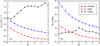 |
Fig. 7 Median values of uncertainties in geocentric speed, σ(υɡ) (panel a) and in the radiant elongation, σ(ϵɡ) (panel b), computed over the subset of hyperbolic events as a function of the confidence level and expressed as Nσ (see Sect. 4.2) in the respective databases (see also Fig. 5). |
Acknowledgements
This work was supported by the Slovak Grant Agency for Science - VEGA, grant No. 2/0009/22. This research made use of NASA’s Astrophysics Data System Bibliographic Services. The authors are very grateful to the anonymous reviewer for the useful comments that helped to improve and clarify the manuscript, and to Chiara Lamberti for the language revision of the entire manuscript.
Appendix A Hyperbolic meteors
An open heliocentric orbit (i.e. a hyperbolic heliocentric speed) is the only readily determinable property of a particle able to possibly indicate its interstellar origin. In the past, hyperbolic meteors have often been considered to be interstellar in nature. Indeed, in the era of visual observations, the vast majority of events were found to be hyperbolic, thus believed to be of interstellar origin (e.g. Fisher 1928; Öpik 1940). This notion was abandoned after the rise of radio observations (Almond et al. 1951, 1952) and more precise photographic observations (Jacchia & Whipple 1961), and after the re-analysis of old data (Öpik 1956). Later, with the investigation of the quality of the orbits, the percentage of possible interstellar meteoroids kept declining and hyperbolic orbits were mostly associated with measurement errors (see Stohl 1970; Sarma & Jones 1985; Hajduková 1993; Hajdukova 1994). The search for interstellar meteoroids was renewed after the confirmation of the presence of interstellar dust in our Solar System (Grun et al. 1993); however, cases that had been suggested at the time (e.g. Baggaley et al. 1993; Baggaley 2000) have since not yet been confirmed or disputed (e.g. Hawkes & Woodworth 1997; Murray et al. 2004). However, there is still a large number of hyperbolic orbits in new and more recent databases (see Tab. 1) and the topic is once again gaining attention within the scientific community. Nevertheless, it is important to be careful when examining meteor databases, for example when searching for interstellar meteoroids, since low-quality orbits might play a significant role in skewing the analysis results.
A.1 Meteor measurements and hyperbolic orbits
There are many reasons, within the data reduction pipeline, why the orbit of a meteoroid can appear hyperbolic. The problems start with the precision and accuracy of meteor measurements and persist in the software used for determining the atmospheric trajectory and computing the heliocentric orbit. Each step of the pipeline introduces a potential source of error, primarily altering the resulting velocity of a meteoroid before its encounter with the Earth (see Sect. 2.2). It has been shown that the vast majority of apparently hyperbolic meteors exhibit significant deviations in at least one of their velocity components compared to the bulk of the observed distribution of meteors (Hajduková et al. 2024).
Hereafter, we provide an example of how an incorrect measurement method can result in a hyperbolic velocity. Whether the measurement is automatic or manual, the measurement technique can greatly affect the resulting meteor velocity and heliocentric orbit. This is particularly important in the case of video recordings. It should be noted that blooming affects the final appearance of stars or meteors. The stars are not shown as dots but as circles of different diameters, and the same applies to the meteor images. To this respect, it is possible to imagine the meteor trail as a thick line with a width of several pixels, depending on the brightness and angular speed of the meteor itself.
Let us illustrate, with an example, the importance of correctly marking the position of the meteor on an image. In order to do so, we used a real meteor observation, recorded by a video camera with an image intensifier (further details can be found in Koten et al. 2020). Figure A.1 shows two measured front points in the same video frame. In this phase, the meteor is relatively bright, therefore its image is bloomed. The correctly measured position of the meteor is displayed in the left panel, taking blooming into account. It is not the exact front of the meteor head that is marked as the position of the meteor (as shown on the right panel). Instead, it should be the centre of the circle fitted to the head of the meteor to be marked as such.
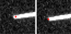 |
Fig. A.1 Correct and incorrect measurements of the meteor position for optical video observations shown for meteor no. 18420521 from Koten et al. (2020). The left panel shows the measurement of the position of the meteor taking into account the image blooming effect, while the right panel shows the exact position of the front of the meteor. |
Radiant and heliocentric orbit (J2000.0) of meteor no. 18420521 from Koten et al. (2020), derived from two distinct measurements (see Fig. A.1).
The measured meteor no. 18420521 was observed by two stations at 22:01:14 UT on 20th April 2018. All the positions of said meteor were measured twice according to the aforementioned methods. Then, we calculated the corresponding atmospheric trajectories and the heliocentric orbits. The results of both correct and incorrect measurements are shown in Tab. A.1. Despite the relatively small difference between the two orbits, we can clearly see that the first measurement method led to a bound heliocentric orbit, whereas the second one led to a hyperbolic orbit. Furthermore, the coordinates of the radiant are somewhat shifted. In particular, the declination angle differs by almost 1°.
This example also demonstrates that the uncertainty (e.g. in the geocentric speed) reflects the measurement precision, which is the same both in the correct and the incorrect measurements, rather than the accuracy of the values. Obviously, the absolute accuracy of the speed is lower in the incorrect measurement than it is in the correct one. In general, the precision of meteor parameters reflects the dispersion in their measurements and calculations within the data-reduction pipelines and depends on the adopted procedures. Furthermore, the precision of meteor parameters varies across different databases, and the uncertainties of the parameters often do not represent the actual limits within which they can be considered accurate. This raises another major challenge, namely, performing a reliable estimation of meteor parameter uncertainties.
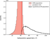 |
Fig. A.2 Distribution of heliocentric speed of real meteoroid population from the GMN database (filled histogram) and distribution of heliocentric speed at the Earth’s distance of hypothetical interstellar meteoroid population (empty histogram). The latter represents the speed distribution at the edge of the Solar System, which mimics the speed distribution of nearby stars. The number of hypothetical interstellar particles considered here equals to the number of hyperbolic events in the observed GMN population. The parabolic limit is marked with a red line. |
It needs to be noted that, especially in automatic pipelines, hyperbolic orbits are often a result of rougher errors. This is often dependent on the quality of measurement devices, technical difficulties (e.g. timing issues), filtering of false events (e.g. flashes, satellite detections) or the presence of outliers in meteor tracks.
A.2 Distribution of hyperbolic speeds
When examining the distribution of the heliocentric speed of meteoroids, υh, it is usually possible to observe a continuous range of values extending beyond the parabolic limit. Conversely, if hyperbolic meteors represented interstellar particles, it should be possible to observe a small secondary peak around 46–49 km s−1 in the histogram of heliocentric speeds (Hajduková et al. 2019). The rationale is that a theoretical population of interstellar particles should reflect the distribution of the relative velocities of the nearby stars (local standard of rest), given that their interaction with the interstellar grains is negligible. Depending on factors such as the spectral type (Dehnen & Binney 1998) and the ejection velocity (Murray et al. 2004), the arrival velocities of interstellar particles at the edge of the Solar System would be on the order of tens of kilometres per second. Consequently, the distribution of their heliocentric excess speed measured at the Earth’s distance should reach a maximum at about a few kilometres per second above the parabolic speed, υp (Hajduková et al. 2019). In other words, the υh-distribution should exhibit two distinct populations: the local elliptical meteoroid population and the interstellar hyperbolic population, which is yet to be observed in any type of data.
In Fig. A.2 we show the sporadic meteor data retrieved from the GMN database (filled histogram) and the first rough approximation of a hypothetical interstellar meteoroid population (empty histogram). For the distribution of this hypothetical population, we used the velocities of the stars from the XHIP catalogue (Anderson & Francis 2012). In particular, a set of 1 358 heliocentric velocity data from stars within a 25 pc distance with < 10% accuracy (Mamajek 2017) was extracted from the catalogue, and a new dataset of such velocities was generated based on the kernel density estimation applied to the distribution of the velocities of the stars. These represent the velocities of the particles at the edge of our Solar System. In Fig. A.2, we recalculated them to the values of heliocentric speed at the Earth’s distance. The number of generated particles is equal to the number of all the hyperbolic meteors of GMN. If this hypothetical population were observed as meteors, the errors from the meteor observation should be accounted for in the empty histogram, which would result in the speed distribution extending into the area below the parabolic limit.
A more accurate model of the interstellar population observed at the Earth’s distance would require accounting for its dynamical evolution within the Solar System caused by the Sun’s gravity (and, for dust particles, also by the solar radiation effects). In particular, we should consider the weighted velocity distribution of interstellar particles approaching the region of inner planets of the Solar System, without which high-speed particles are favoured. On the other hand, the focusing effect is more effective on slower particles approaching the Sun, thus favouring low-speed interstellar particles. Such an approach can be found in Strub et al. (2019), who modelled the interstellar dust flow onto the Earth, and in Baggaley & Neslušan (2002), who modelled the heliocentric orbits of Earth-intersecting meteoroids of a theoretical interstellar stream. These works also demonstrated that variations in the collision geometry due to changes in the Earth’s heliocentric longitude lead to variations in the orbital elements of the modelled interstellar particles. However, the aim of our paper is not to create the most accurate model of the hypothetical interstellar population, but rather to highlight that the observed hyperbolic population does not exhibit its expected properties if interpreted as of interstellar origin.
A.3 Hyperbolic shower meteors
Another argument against considering hyperbolic orbits as real interstellar events is the presence of stream meteoroids among them. If a meteor shower is associated with a parent body originated in our Solar System, then the hyperbolic stream meteoroids that are associated with it are most likely the results of errors (Hajduková et al. 2014; Hajduková & Kornoš 2020). Of course, it is possible for the meteoroids to be accelerated to hyper-bolic orbits, either being ejected from long-period near-parabolic comets or due to planetary scattering; nevertheless, the number of such cases should be negligible (Wiegert 2014).
That the data regarding the present hyperbolic orbits among stream meteoroids are erroneous is supported by the dependence of their numbers on individual meteoroid streams and on the mean heliocentric speed of the stream Ne>1 /N = f (υh), as already reported by Hajduková (2008). In Figs. A.3 and A.4, we illustrate this dependence for the meteor showers identified in the CAMS, GMN and FRIPON databases. Only those meteor showers with ten or more identified members are shown in the graphs. Figure A.3 shows meteor showers taken from the GMN and the CAMS databases, for which cases the shower association was taken directly from the given datasets. Figure A.4 displays meteor showers identified from the FRIPON database and a selection of 9 662 meteor orbits of magnitude brighter than −3 from the GMN data. The selection operated on the GMN dataset is the one that best corresponds to the FRIPON data according to its limiting magnitude. The meteor showers in these graphs were identified via a modified version of the independent identification method of Rudawska et al. (2015), as described in Durišová et al. (2023). A DS H-criterion (Southworth & Hawkins 1963) was used to determine the orbital similarity with a threshold value of 0.15 (e.g. Drummond 1991; Moorhead 2016).
 |
Fig. A.3 Dependence of the percentage of hyperbolic orbits on the individual meteoroid stream and on the mean heliocentric speed of the stream for (a) the CAMS and (b) the GMN databases. The red line indicates a value of 42.1 km s−1 of heliocentric speed, that is the mean value of the parabolic limit. The individual points representing meteoroid streams (and their corresponding meteor showers) are colour-coded based on the calculated value of the mean geocentric speed of the shower. |
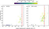 |
Fig. A.4 Dependence of the percentage of hyperbolic orbits on the individual meteoroid stream and on the mean heliocentric speed of the stream for (a) the FRIPON database and (b) a subset of the GMN database, which contains events with magnitude less than −3 (see Fig. A.3 for further details). |
It is also important to highlight how the high dispersion of the points shown in Figs. A.3 and A.4 may originate from the low quality of meteoroid stream parameters, especially when dealing with poorly-determined orbits. This is particularly true for minor meteor showers with a small number of associated events and high geocentric speeds.
References
- Almond, M., Davies, J. G., & Lovell, A. C. B. 1951, MNRAS ,111, 585 [CrossRef] [Google Scholar]
- Almond, M., Davies, J. C., & Lovell, A. C. B. 1952, MNRAS ,112, 21 [CrossRef] [Google Scholar]
- Anderson, E., & Francis, C. 2012, Astron. Lett. ,38, 331 [Google Scholar]
- Baggaley, W. J. 2000, J. Geophys. Res. ,105, 10353 [NASA ADS] [CrossRef] [Google Scholar]
- Baggaley, W. J., & Neslušan, L. 2002, A&A ,382, 1118 [NASA ADS] [CrossRef] [EDP Sciences] [Google Scholar]
- Baggaley, W. J., Taylor, A. D., & Steel, D. I. 1993, in Meteoroids and their Parent Bodies, eds. J. Stohl, & I. P. Williams, 53 [Google Scholar]
- Balis, J., Lamy, H., Anciaux, M., & Jehin, E. 2023, Radio Sci., 58, e2023RS007697 [Google Scholar]
- Barghini, D. 2023, PhD thesis, University of Turin, Physics Department, Italy [Google Scholar]
- Barghini, D., Gardiol, D., & Carbognani, A. 2019, in International Meteor Conference, Pezinok-Modra, Slovakia, eds. R. Rudawska, J. Rendtel, C. Powell, et al., 41 [Google Scholar]
- Borovicka, J. 1990, Bull. Astron. Inst. Czech. ,41, 391 [NASA ADS] [Google Scholar]
- Borovicka, J., Spurny, P., & Keclikova, J. 1995, A&AS ,112, 173 [Google Scholar]
- Borovicka, J., Spurný, P., & Shrbený, L. 2022a, A&A ,667, A158 [NASA ADS] [CrossRef] [EDP Sciences] [Google Scholar]
- Borovicka, J., Spurný, P., Shrbený, L., et al. 2022b, A&A, 667, A157 [NASA ADS] [CrossRef] [EDP Sciences] [Google Scholar]
- Brož, M., Vernazza, P., Marsset, M., et al. 2024, Nature, 634, 566 [Google Scholar]
- Brown, P., Spalding, R. E., ReVelle, D. O., Tagliaferri, E., & Worden, S. P. 2002, Nature, 420, 294 [Google Scholar]
- Brown, P., Jones, J., Weryk, R. J., & Campbell-Brown, M. D. 2004, Earth Moon Planets, 95, 617 [Google Scholar]
- Ceplecha, Z. 1987, Bull. Astron. Inst. Czech. ,38, 222 [NASA ADS] [Google Scholar]
- Clark, D. L., & Wiegert, P. A. 2011, maps, 46, 1217 [Google Scholar]
- Colas, F., Zanda, B., Bouley, S., et al. 2020, A&A, 644, A53 [EDP Sciences] [Google Scholar]
- Dehnen, W., & Binney, J. J. 1998, MNRAS ,298, 387 [NASA ADS] [CrossRef] [Google Scholar]
- Devillepoix, H. A. R., Bland, P. A., Sansom, E. K., et al. 2019, MNRAS, 483, 5166 [NASA ADS] [CrossRef] [Google Scholar]
- Devillepoix, H. A. R., Cupák, M., Bland, P. A., et al. 2020, Planet. Space Sci., 191, 105036 [Google Scholar]
- Dmitriev, V., Lupovka, V., & Gritsevich, M. 2015, Planet. Space Sci. ,117, 223 [Google Scholar]
- Drummond, J. D. 1991, Icarus ,89, 14 [Google Scholar]
- Dubyago, A. D. 1961, The Macmillan Company, New York, USA [Google Scholar]
- Durišová, S., Tóth, J., & Hajduková, M. 2023, Planet. Space Sci. ,236, 105752 [Google Scholar]
- Egal, A., Vaubaillon, J., Colas, F., & Atreya, P. 2014, in Proceedings of the International Meteor Conference, Giron, France, 18-21 September 2014, eds. J. L. Rault, & P. Roggemans, 49 [Google Scholar]
- Fisher, W. J. 1928, Harvard Coll. Observ. Circ. ,331, 1 [Google Scholar]
- Gardiol, D., Affaticati, F., Albani, M., et al. 2019, in Proceedings of the 37th International Meteor Conference, Pezinok-Modra, Slovakia, 30 August- 2 September 2018, eds. R. Rudawska, J. Rendtel, C. Powell, et al. 81 [Google Scholar]
- Gardiol, D., Cellino, A., & Di Martino, M. 2016, in Proceedings of the 35th International Meteor Conference, Egmond, the Netherlands, 2-5 June 2016, eds. A. Roggemans, & P. Roggemans, 76 [Google Scholar]
- Gardiol, D., Barghini, D., Buzzoni, A., et al. 2021, MNRAS, 501, 1215 [Google Scholar]
- Granvik, M., & Brown, P. 2018, Icarus ,311, 271 [Google Scholar]
- Gritsevich, M., & Koschny, D. 2011, Icarus ,212, 877 [CrossRef] [Google Scholar]
- Gritsevich, M. I. 2009, Adv. Space Res. ,44, 323 [NASA ADS] [CrossRef] [Google Scholar]
- Grun, E., Zook, H. A., Baguhl, M., et al. 1993, Nature, 362, 428 [Google Scholar]
- Gural, P. S. 2012, maps, 47, 1405 [Google Scholar]
- Hajduková, M., J. 1993, in Meteoroids and their Parent Bodies, eds. J. Stohl, & I. P. Williams, 61 [Google Scholar]
- Hajdukova, M., J. 1994, A&A, 288, 330 [Google Scholar]
- Hajduková, M. 2008, Earth Moon Planets ,102, 67 [Google Scholar]
- Hajduková, M., & Kornoš, L. 2020, Planet. Space Sci. ,190, 104965 [CrossRef] [Google Scholar]
- Hajduková, M., J., Kornoš, L., & Tóth, J. 2014, in Meteoroids 2013, eds. T. J. Jopek, F. J. M. Rietmeijer, J. Watanabe, & I. P. Williams, 289 [Google Scholar]
- Hajduková, M., Sterken, V., & Wiegert, P. 2019, in Meteoroids: Sources of Meteors on Earth and Beyond, eds. G. O. Ryabova, D. J. Asher, & M. J. Campbell-Brown (Cambridge University Press), 235 [Google Scholar]
- Hajduková, M., Sterken, V., Wiegert, P., & Kornoš, L. 2020, Planet. Space Sci., 192, 105060 [NASA ADS] [CrossRef] [Google Scholar]
- Hajduková, M., Stober, G., Barghini, D., et al. 2024, A&A, 691, A8 [NASA ADS] [CrossRef] [EDP Sciences] [Google Scholar]
- Hawkes, R. L., & Woodworth, S. C. 1997, JRASC ,91, 68 [Google Scholar]
- Jacchia, L. G., & Whipple, F. L. 1961, Smithsonian Contrib. Astrophys. ,4, 97 [CrossRef] [Google Scholar]
- Jansen-Sturgeon, T., Sansom, E. K., & Bland, P. A. 2019, Meteorit. Planet. Sci. ,54, 2149 [NASA ADS] [CrossRef] [Google Scholar]
- Jeanne, S., Colas, F., Zanda, B., et al. 2019, A&A, 627, A78 [EDP Sciences] [Google Scholar]
- Jenniskens, P. 2006, Meteor Showers and their Parent Comets (Cambridge University Press) [Google Scholar]
- Jenniskens, P., Gural, P. S., Dynneson, L., et al. 2011, Icarus, 216, 40 [NASA ADS] [CrossRef] [Google Scholar]
- Jenniskens, P., Nénon, Q., Albers, J., et al. 2016, Icarus, 266, 331 [NASA ADS] [CrossRef] [Google Scholar]
- Jenniskens, P., Utas, J., Yin, Q.-Z., et al. 2019, Meteorit. Planet. Sci., 54, 699 [Google Scholar]
- Jenniskens, P., Moskovitz, N., Garvie, L. A. J., et al. 2020, Meteorit. Planet. Sci., 55, 535 [Google Scholar]
- Kastinen, D., & Kero, J. 2022, MNRAS ,517, 3974 [Google Scholar]
- Khanukaeva, D. Y. 2004, Earth Moon Planets ,95, 433 [Google Scholar]
- Kornoš, L., Koukal, J., Piffl, R., & Tóth, J. 2014, in Proceedings of the International Meteor Conference, Poznan, Poland, 22-25 August 2013, eds. M. Gyssens, P. Roggemans, & P. Zoladek, 23 [Google Scholar]
- Koten, P., Spurný, P., Borovicka, J., & Stork, R. 2003, Publ. Astron. Inst. Czech. Acad. Sci., 91, 1 [Google Scholar]
- Koten, P., Borovicka, J., Vojácek, V., et al. 2020, Planet. Space Sci., 184, 104871 [NASA ADS] [CrossRef] [Google Scholar]
- Kresák, L., & Kresáková, M. 1976, Bull. Astron. Inst. Czech. ,27, 106 [Google Scholar]
- Lyytinen, E., & Gritsevich, M. 2016, Planet. Space Sci. ,120, 35 [Google Scholar]
- Madiedo, J. M., & Trigo-Rodríguez, J. M. 2008, Earth Moon Planets ,102, 133 [Google Scholar]
- Mamajek, E. 2017, RNAAS ,1, 21 [NASA ADS] [Google Scholar]
- McKinley, D. W. R. 1961, Meteor Science and Engineering. (McGraw-Hill) [Google Scholar]
- McMullan, S., Vida, D., Devillepoix, H. A. R., et al. 2024, Meteorit. Planet. Sci., 59, 927 [Google Scholar]
- Millman, P. M., & McKinley, D. W. R. 1963, Meteors (Chicago: The University of Chicago Press), 674 [Google Scholar]
- Moorhead, A. V. 2016, MNRAS ,455, 4329 [CrossRef] [Google Scholar]
- Moorhead, A. V., Brown, P. G., Campbell-Brown, M. D., Heynen, D., & Cooke, W. J. 2017, Planet. Space Sci., 143, 209 [Google Scholar]
- Murray, N., Weingartner, J. C., & Capobianco, C. 2004, ApJ ,600, 804 [NASA ADS] [CrossRef] [Google Scholar]
- Nedelcu, D. A., Birlan, M., Turcu, V., et al. 2018, Romanian Astron. J., 28, 57 [NASA ADS] [Google Scholar]
- Neslušan, L., Porubcan, V., & Svoren, J. 2014, Earth Moon Planets ,111, 105 [CrossRef] [Google Scholar]
- Öpik, E. 1940, Publ. Tartu Astrofiz. Observ. ,30, E1 [Google Scholar]
- Öpik, E. J. 1956, Irish Astron. J. ,4, 49 [Google Scholar]
- Peña-Asensio, E., Trigo-Rodríguez, J. M., Gritsevich, M., & Rimola, A. 2021, MNRAS, 504, 4829 [Google Scholar]
- Pecina, P., & Ceplecha, Z. 1983, Bull. Astron. Inst. Czech. ,34, 102 [NASA ADS] [Google Scholar]
- Roggemans, P., Campbell-Burns, P., Kalina, M., et al. 2024, eMeteorNews, 9, 56 [Google Scholar]
- Rudawska, R., Matlovic, P., Tóth, J., & Kornoš, L. 2015, Planet. Space Sci., 118, 38 [NASA ADS] [CrossRef] [Google Scholar]
- Sansom, E. K., Jansen-Sturgeon, T., Rutten, M. G., et al. 2019, Icarus, 321, 388 [Google Scholar]
- Sarma, T., & Jones, J. 1985, Bull. Astron. Inst. Czech. ,36, 9 [NASA ADS] [Google Scholar]
- Shober, P. M., Vaubaillon, J., Anghel, S., et al. 2023, in LPI Contributions, 2851, Asteroids, Comets, Meteors Conference, 2402 [Google Scholar]
- Skokic, I., Šegon, D., & Kurtovic, G. 2016, in International Meteor Conference, Egmond, the Netherlands, 2-5 June 2016, eds. A. Roggemans, & P. Roggemans, 280 [Google Scholar]
- SonotaCo. 2009, WGN, JIMO, 37, 55 [NASA ADS] [Google Scholar]
- SonotaCo. 2016, WGN, JIMO, 44, 42 [Google Scholar]
- Southworth, R. B., & Hawkins, G. S. 1963, Smithsonian Contrib. Astrophys. ,7, 261 [Google Scholar]
- Spurný, P., Borovicka, J., Mucke, H., & Svoren, J. 2017, A&A, 605, A68 [NASA ADS] [CrossRef] [EDP Sciences] [Google Scholar]
- Spurný, P., Borovicka, J., & Shrbený, L. 2020, Meteorit. Planet. Sci. ,55, 376 [CrossRef] [Google Scholar]
- Stohl, J. 1970, Bull. Astron. Inst. Czech. ,21, 10 [NASA ADS] [Google Scholar]
- Strub, P., Sterken, V. J., Soja, R., et al. 2019, A&A, 621, A54 [NASA ADS] [CrossRef] [EDP Sciences] [Google Scholar]
- Vida, D., Brown, P. G., Campbell-Brown, M., Wiegert, P., & Gural, P. S. 2020a, MNRAS, 491, 3996 [NASA ADS] [CrossRef] [Google Scholar]
- Vida, D., Gural, P. S., Brown, P. G., Campbell-Brown, M., & Wiegert, P. 2020b, MNRAS, 491, 2688 [NASA ADS] [CrossRef] [Google Scholar]
- Vida, D., Brown, P. G., Campbell-Brown, M., et al. 2021a, Icarus, 354, 114097 [CrossRef] [Google Scholar]
- Vida, D., Šegon, D., Gural, P. S., et al. 2021b, MNRAS, 506, 5046 [NASA ADS] [CrossRef] [Google Scholar]
- Wiegert, P. A. 2014, Icarus ,242, 112 [NASA ADS] [CrossRef] [Google Scholar]
- Wiegert, P., Vaubaillon, J., & Campbell-Brown, M. 2009, Icarus ,201, 295 [NASA ADS] [CrossRef] [Google Scholar]
- Wiegert, P., Tran, V., Gregg, C., Vida, D., & Brown, P. 2025, ApJ, 984, 151 [Google Scholar]
When υ∞ = 50 km s−1, v0 = 30 km s−1, and υh = 36–42 km s−1, the angle between the heliocentric velocity vector and the Earth’s velocity vector ranges from 83.5° to a maximum of 95°.
From its mathematical definition,  . However, it is physically unreasonable to think that any event would survive a selection with an indefinitely large confidence level. In practice, ƒ0 is the fraction of hyperbolic events that survive the highest confidence level considered; for example, when giving an estimation of the upper limit of the flux of interstellar meteoroids.
All Tables
Radiant and heliocentric orbit (J2000.0) of meteor no. 18420521 from Koten et al. (2020), derived from two distinct measurements (see Fig. A.1).
All Figures
|
Fig. 1 Density maps of values of standard error, σ(υɡ), as function of geocentric speed, υɡ, for databases used in this study (see Table 1). In all panels, the solid coloured line plots the result of a linear fit in the linear-log space, and the dashed coloured lines mark the corresponding prediction band at a 68% confidence level. |
| In the text | |
|
Fig. 2 Visualisation of the Kresáks’ diagram, showing relationship between geocentric meteor parameters and resulting heliocentric meteoroid orbits. The different dashed black lines represent orbits with varying values of semi-major axes (see legend of panel b), and the red lines plot the parabolic limit. Panel a displays the position on the Kresáks’ diagram of simplified areas corresponding to the orbit type of each event shown in the graph. Panels b and c demonstrate the approach using older photographic meteors reported in eight IAU MDC catalogues. Panel b represents all photographic catalogues together, with the parabolic limit dividing the diagram into two regions, which are those of meteoroids on elliptical orbits (grey crosses) and hyperbolic orbits (red crosses), showing a continuous spread between the two (Hajduková et al. 2019). Panel c displays the photographic orbits colour-coded according to their respective catalogues and reflecting their data quality. Hereafter, the selected catalogues and their labels in panels b and c are as follows: C – 103 orbits, Ceplecha’s small camera; D – 636 orbits, Dushanbe stations; E – 180 orbits, European Network; J – 413 orbits, Harvard Super Schmidt camera; K – 206 orbits, Kiev stations; O – 459 orbits, Odessa stations; R – 32 orbits, Spanish meteor society; and W – 166 orbits, Harvard small cameras. |
| In the text | |
|
Fig. 3 Visualisation of confidence regions for geocentric quantities on the Kresáks’ diagram for two simulated meteors. In both panels, the parameters of the observed meteor were generated as υ∞ = (65.7 ± 0.4) km s−1, α = (153 ± 1)°, and δ = (5 ± 1)°. The corresponding nominal values and standard errors for υɡ and ϵɡ are reported as cyan error bars. The blue ellipses, from inner to outer, show the boundaries of the 1σ, 2σ, and 3σ confidence regions, and the red line plots the parabolic limit. The black dots represent the result of a bootstrap Monte Carlo error propagation for an ensemble of 300 repetitions. The simulation included a covariance matrix element for (υ∞, α) of +0.3 for panel a and of −0.3 for panel b. |
| In the text | |
|
Fig. 4 Density representation of the Kresáks’ diagram for databases of (a) FRIPON, (b) GMN, (c) EFN, (d) Ondřejov, (e) CNEOS, and (f) CAMS, given in logarithmic greyscale. The red curve plots the parabolic limit, and the red crosses represent hyperbolic events that overpass such limit with a p value lower than 0.14% (3σ). Each panel also displays the percentage of hyperbolic (black) and 3σ hyperbolic (red) events. |
| In the text | |
|
Fig. 5 Significance of hyperbolic orbits in the FRIPON, GMN and CAMS meteor databases. Panel a shows the fraction of hyperbolic events as a function of the confidence level expressed as Nσ, which represents the number of standard deviations used to define the confidence interval in the Kresáks’ diagram. The coloured curves represent the fitting of Eq. (3) over the results of each database. Panel b displays the fraction of meteors associated with known meteor showers belonging to the hyperbolic subset as a function of Nσ. |
| In the text | |
|
Fig. 6 Distributions of uncertainties in geocentric speed, σ(υɡ), (panels a, c, and e) and in radiant elongation, σ(ϵɡ), (panels b, d, and f) as reported in the respective databases (i.e. FRIPON, GMN, and CAMS, the three largest ones considered in this study). Distributions are shown separately for all events (filled histograms) and for hyperbolic events that survived the 3σ filtering (empty histograms). |
| In the text | |
|
Fig. 7 Median values of uncertainties in geocentric speed, σ(υɡ) (panel a) and in the radiant elongation, σ(ϵɡ) (panel b), computed over the subset of hyperbolic events as a function of the confidence level and expressed as Nσ (see Sect. 4.2) in the respective databases (see also Fig. 5). |
| In the text | |
|
Fig. A.1 Correct and incorrect measurements of the meteor position for optical video observations shown for meteor no. 18420521 from Koten et al. (2020). The left panel shows the measurement of the position of the meteor taking into account the image blooming effect, while the right panel shows the exact position of the front of the meteor. |
| In the text | |
|
Fig. A.2 Distribution of heliocentric speed of real meteoroid population from the GMN database (filled histogram) and distribution of heliocentric speed at the Earth’s distance of hypothetical interstellar meteoroid population (empty histogram). The latter represents the speed distribution at the edge of the Solar System, which mimics the speed distribution of nearby stars. The number of hypothetical interstellar particles considered here equals to the number of hyperbolic events in the observed GMN population. The parabolic limit is marked with a red line. |
| In the text | |
|
Fig. A.3 Dependence of the percentage of hyperbolic orbits on the individual meteoroid stream and on the mean heliocentric speed of the stream for (a) the CAMS and (b) the GMN databases. The red line indicates a value of 42.1 km s−1 of heliocentric speed, that is the mean value of the parabolic limit. The individual points representing meteoroid streams (and their corresponding meteor showers) are colour-coded based on the calculated value of the mean geocentric speed of the shower. |
| In the text | |
|
Fig. A.4 Dependence of the percentage of hyperbolic orbits on the individual meteoroid stream and on the mean heliocentric speed of the stream for (a) the FRIPON database and (b) a subset of the GMN database, which contains events with magnitude less than −3 (see Fig. A.3 for further details). |
| In the text | |
Current usage metrics show cumulative count of Article Views (full-text article views including HTML views, PDF and ePub downloads, according to the available data) and Abstracts Views on Vision4Press platform.
Data correspond to usage on the plateform after 2015. The current usage metrics is available 48-96 hours after online publication and is updated daily on week days.
Initial download of the metrics may take a while.