| Issue |
A&A
Volume 701, September 2025
|
|
|---|---|---|
| Article Number | A142 | |
| Number of page(s) | 16 | |
| Section | Extragalactic astronomy | |
| DOI | https://doi.org/10.1051/0004-6361/202554367 | |
| Published online | 08 September 2025 | |
Rates of strongly lensed tidal disruption events
A comprehensive investigation of black hole, luminosity, and temperature dependencies
1
Technical University of Munich, TUM School of Natural Sciences, Physics Department, James-Franck-Straße 1, 85748 Garching, Germany
2
Max Planck Institute for Astrophysics, Karl-Schwarzschild Str. 1, 85748 Garching, Germany
3
JILA, University of Colorado and National Institute of Standards and Technology, 440 UCB, Boulder, 80308 CO, USA
4
Department of Astrophysical and Planetary Sciences, 391 UCB, Boulder, 80309 CO, USA
5
Department of Astronomy and Astrophysics, and Institute for Gravitation and the Cosmos, Pennsylvania State University, 525 Davey Lab, 251 Pollock Road, University Park, PA 16802, USA
6
Department of Physics, University of Hong Kong, Pokfulam Road, Hong Kong, PR, China
7
Center for Frontier Science, Chiba University, 1-33 Yayoicho, Inage, Chiba 263-8522, Japan
8
Department of Physics, Graduate School of Science, Chiba University, 1-33 Yayoicho, Inage, Chiba 263-8522, Japan
⋆ Corresponding author: This email address is being protected from spambots. You need JavaScript enabled to view it.
; This email address is being protected from spambots. You need JavaScript enabled to view it.
Received:
4
March
2025
Accepted:
9
July
2025
Abstract
In the coming years, surveys such as the Rubin Observatory’s Legacy Survey of Space and Time (LSST) are expected to increase the number of observed Tidal Disruption Events (TDEs) substantially. We employed Monte Carlo integration to calculate the unlensed and lensed TDE rate as a function of limiting magnitude in the u, g, r, and i bands. We investigated the impact of multiple luminosity models, black hole mass functions (BHMFs), and flare temperatures on the TDE rate. Notably, this includes a semi-analytical model, which enables the determination of the TDE temperature in terms of (BH) mass. We predict the highest unlensed TDE rate to be in the g band. It ranges from 16 to 5440 yr−1 (20 000 deg2)−1 for the (ZTF), and it is more consistent with the observed rate at the low end. For LSST, we expect a rate in the g band between 3580 and 82 060 yr−1 (20 000 deg2)−1. A higher theoretical prediction is within reason, as we do not consider observational effects such as completeness. The unlensed and lensed TDE rates are insensitive to the redshift evolution of the BHMF, even for LSST limiting magnitudes. The best band for detecting lensed TDEs is also the g band. Its predicted rates range from 0.43 to 15 yr−1 (20 000 deg2)−1 for LSST. The scatter of predicted rates reduces when we consider the fraction of lensed TDEs; that is, only a few in ten thousand TDEs will be lensed. Despite the large scatter in the rates of lensed TDEs, our comprehensive considerations of multiple models suggest that lensed TDEs will occur in the 10-year LSST lifetime, providing an exciting prospect for detecting such events. We expect the median redshift of a lensed TDE to be between 1.5 and 2. In this paper, we additionally report on lensed TDE properties, such as the BH mass and time delays.
Key words: gravitational lensing: strong / methods: numerical / Galaxy: nucleus / black hole physics
© The Authors 2025
 Open Access article, published by EDP Sciences, under the terms of the Creative Commons Attribution License (https://creativecommons.org/licenses/by/4.0), which permits unrestricted use, distribution, and reproduction in any medium, provided the original work is properly cited.
This article is published in open access under the Subscribe to Open model.
Open access funding provided by Max Planck Society.
1. Introduction
When a star ventures too close to a (BH), tidal forces tear it apart. We can observe such an event as a bright transient, a so-called Tidal Disruption Event (TDE; Hills 1988; Rees 1988). These events typically last one to two years for main sequence stars (e.g., Gezari 2021), but in rare cases, they can extend much longer than that (Lin et al. 2017). TDEs are multi-messenger transients that produce electromagnetic radiation (e.g., Komossa et al. 2004; Gezari et al. 2009), neutrinos (e.g., Reusch et al. 2022; Wevers & Ryu 2023), and gravitational wave signatures (e.g., Toscani et al. 2020; Pfister et al. 2022; Wevers & Ryu 2023). Even today, by analyzing the light of the TDE, we can infer critical properties such as the mass of the BHs and the disrupted stars (e.g., Ryu et al. 2020a) and gain insights into BH demographics and accretion physics (e.g., Rees 1988; Gezari 2013). Understanding TDE rates and their observational characteristics is vital for detecting them in current and future surveys such as the Zwicky Transient Facility (ZTF; Wozniak et al. 2014) and the Rubin Observatory’s Legacy Survey of Space and Time (LSST; Ivezić et al. 2019). Estimating the rate of TDEs across different survey depths allows for better planning of observational campaigns and the design of strategies to maximize scientific returns (e.g., Bricman & Gomboc 2020; Lin et al. 2022).
A key advancement in this area of study is the inclusion of lensed TDEs in our analysis. Gravitational lensing provides a powerful mechanism to magnify and detect TDEs from deep within the cosmos. This topic has already been studied with electromagnetic radiation in Szekerczes et al. (2024) and Chen et al. (2024), upon which we expand here. In the future, we could also expect gravitational waves to be lensed. This has, for example, been studied by Toscani et al. (2023). Beyond enhancing detectability, lensing offers the potential to probe cosmological parameters such as the Hubble constant (Refsdal 1964) and the size of the emission region via microlensing effects, as demonstrated for active galactic nuclei (e.g., Rauch & Blandford 1991; Yonehara et al. 1999; Kochanek 2004). Despite these promising applications, the abundance and characteristics of TDEs, lensed or unlensed, remain uncertain (e.g., Gomez et al. 2023). Addressing this gap, we calculated the TDE rate for various models and assessed whether these events are numerous enough to serve as a tool for future research.
In this work, we employed Monte Carlo simulations to calculate TDE rates as a function of limiting magnitude, following the methodology of Szekerczes et al. (2024). Likewise, we generated mock catalogs to analyze the population of unlensed and lensed TDEs. Estimating the TDE rate requires two primary components: a TDE luminosity model and the black hole mass function (BHMF). Building on the calculations of Szekerczes et al. (2024), in addition to the phenomenological fit model (Thomsen et al. 2022), we incorporated the full semi-analytical stream-stream collision model for TDEs (Piran et al. 2015; Ryu et al. 2020a). This model enables the determination of the TDE temperature as a function of BH mass, eliminating the need to assume a temperature. In addition to the local BHMF adopted in Szekerczes et al. (2024), we included two more BHMFs that account for redshift dependence, enhancing the accuracy of our predictions. For lensed TDEs, we also investigated the fraction of TDEs that are lensed for the different models, leading to a more robust forecast.
The structure of the paper is as follows: In Sect. 2, we provide an overview of the relevant theoretical background, focusing on the TDE models used to calculate the TDE magnitude. We also detail our methodology for determining the unlensed TDE rate and extend it to create a mock TDE catalog. Sect. 3 presents the results for the unlensed case, and we analyze the effects of various model parameters and compare them with current observations. In Sect. 4, we shift our focus to the lensed rate, describing the creation of mock catalogs of lensed TDEs. We then explore the lensed TDE rate, the fraction of lensed events, and the parameter distributions for the source TDE, the lens, and the lens system. Finally, we summarize our findings and conclusions in Sect. 5.
2. TDE models and rate derivation
2.1. Rate integral
We followed Szekerczes et al. (2024) in the derivation of the unlensed TDE rate integral
 (1)
(1)
Here NTDE is the number of TDE per year, MBH is the BH mass, Γ is the TDE occurrence rate per galaxy, ϕBH is the BHMF, V is the volume, and z is the redshift. We have already changed the variable from volume to redshift using (e.g., Oguri & Marshall 2010)
 (2)
(2)
where Ω is the solid angle corresponding to the survey area, DL is the luminosity distance, c is the speed of light, and dt/dz = −1/(H ⋅ (1 + z)), where H is the Hubble parameter. We adopted the TDE occurrence rate
 (3)
(3)
In addition to the redshift-independent BHMF (Gallo & Sesana 2019; Wong et al. 2022)
 (4)
(4)
which is illustrated in the left panel of Fig. 1, we investigated two more. First, we included the BHMF derived by the TRINITY model (Zhang et al. 2023). They used a Markov chain Monte Carlo algorithm to fit a star-formation rate to the maximum circular halo velocity relation, a BH-to-bulge mass relation, and an active BH luminosity distribution to observed data. The derived BHMF is shown in the middle panel of Fig. 1. This BHMF displays an almost uniform redshift evolution across the BH mass range. But the evolution only affects the BHMF strongly for z ≳ 2. Second, we considered a BHMF that is calculated by combining the galaxy stellar mass function (GSMF) from Davidzon et al. (2017) and the BH-to-bulge mass relation from Kormendy & Ho (2013)
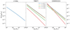 |
Fig. 1. Three different BHMFs we consider showing significantly different redshift evolutions. Left panel: Redshift independent BHMF from Gallo & Sesana (2019). Middle panel: BHMF derived by the TRINITY model (Zhang et al. 2023). Right panel: BHMF calculated by combining a galaxy stellar mass function (GSMF) (Davidzon et al. 2017) and a BH-to-bulge mass relation (Kormendy & Ho 2013). The z-independent BHMF has a different normalization than the other two. Up to redshift of 2, TRINITY and COSMOS2015 agree closely. |
 (5)
(5)
with Mbulge as the galaxy bulge mass. It has recently been suggested that this relation is redshift-dependent (e.g., Shimizu et al. 2024). However, we still assume no redshift dependence because the GSMF, which is fitted in bins to the COSMOS2015 catalog (Laigle et al. 2016), already includes a strong, non-trivial redshift dependence. As illustrated in the right panel of Fig. 1, this BHMF agrees closely with the TRINITY BHMF at z = 0, but not for larger redshifts. From z = 2 onward, the high-mass end decreases, while the low-mass end turns and increases. This is due to the extrapolation needed to reach such low BH masses. The COSMOS2015 catalog only includes data for galaxies of just below 1010 M⊙. This corresponds to a BH mass of 107.5 M⊙, the upper end of our considered mass range. Assuming the fitting function is still valid, we extrapolated the relation down to a BH mass of 105 M⊙.
2.2. Magnitude bounds
The limiting magnitude of the survey gives the bounds to the integral in Eq. (1). Hence, calculating the magnitude of a given TDE is essential. Following Bessell & Murphy (2012), as done in Huber et al. (2021), we calculated the magnitude in a band X:
 (6)
(6)
where λobs is the observed wavelength and SX(λ) is the band transmission function. We used the same rectangular approximations of the LSST transmission functions as Szekerczes et al. (2024). Finally, (e.g., Huber et al. 2021)
 (7)
(7)
is the observed flux for an emitting region of area, A, with a spatially constant emitted specific intensity, Iλobs. We also assumed the TDE to emit as a black body described by the Planck law (Planck 1901)
 (8)
(8)
where λem is the emitted wavelength, T is the temperature, h is the Planck constant, and k is the Boltzmann constant. In addition, the Stefan-Boltzmann law (e.g., Baehr & Kabelac 2016) applies, and it allows us to rewrite the emission area,
 (9)
(9)
in terms of luminosity, L, and the Stefan-Boltzmann constant, σ. The full solution to the integral in the numerator of the magnitude is given in Appendix A.
In the following two subsections, we present two different luminosity models for TDEs. They are similar to the ones considered by Szekerczes et al. (2024).
2.2.1. Phenomenological luminosity model
The first model is an empirical fit between the observed TDE luminosity and the debris fallback rate found by Thomsen et al. (2022):
 (10)
(10)
which assumes that the disrupted star has a stellar mass of 0.1 M⊙. Here
 (11)
(11)
is the mass fallback rate from Ryu et al. (2020b). It depends on the stellar mass, M⋆; the stellar radius, R⋆; an energy correction factor, Ξ, which we explain in more detail in the next section (Sect. 2.2.2); and the correction factor, f, that accounts for different possible shapes of the energy distribution near the tails of the debris. In this first model, the debris energy spread correction factor is omitted, that is, Ξ = 1. The correction factor, f, is equal to 1, for M⋆ ≤ 0.5 M⊙ and f = 0.5 for M⋆ > 0.5 M⊙. Hence, we set f to 1. Additionally, we assumed a stellar radius of 0.15 R⊙. We also limited the luminosity to the Eddington limit (e.g., Rybicki & Lightman 1979):
 (12)
(12)
The first TDE luminosity model, denoted with L1, is then
 (13)
(13)
We show this luminosity in Fig. 2. In this model, we assumed the disk’s temperature to be constant. We refer to this assumption as the temperature-independent case. We performed our calculations for five temperatures, 1, 2, 3, 4, and 5 ⋅ 104 K, covering the observed range of temperatures of optical TDEs (Hammerstein et al. 2023).
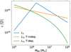 |
Fig. 2. Three different TDE luminosity functions dependent on BH mass. For low BH masses, L1 is Eddington limited. The two L2 models do not yet differ through their treatment of temperature, as temperature is not involved yet. However, they differ because of a correction factor that accounts for the spread of specific energy in the resulting debris. The T-independent model assumes this factor to be constant. |
2.2.2. Theoretical luminosity model
The second model we considered is by Piran et al. (2015), and it was later improved by Ryu et al. (2020a). They propose that shocks within an eccentric accretion flow drive the light emission from a TDE. The shock is formed when earlier arriving debris, after one orbit around the BH, collide with later arriving debris. The peak luminosity,
 (14)
(14)
depends on a0 = (GMBH)/ΔE, which gives the size of the mass flow. Here, G is the gravitational constant, and ΔE is the spread in specific energy. Specifically, it is the apocenter distance of the most-bound debris. Combining Eqs. (11) and (14), we obtained the full expression for the second luminosity model:
 (15)
(15)
We then split this model in two. First, following Szekerczes et al. (2024), we assumed the temperature to be constant at the same values as for L1. Additionally, we assumed all disrupted stars to be solar-like, that is, M⋆ = 1 M⊙ and R⋆ = 1 R⊙, from which follows Ξ = 1.49 and f = 0.5. We call this set of assumptions our temperature-independent L2 model.
The second option is a case where we include the full temperature dependence in this luminosity model. More specifically, we calculated the temperature in terms of BH mass. As this model includes an expression for the (BB) radius, it is possible to calculate an effective emission area,
 (16)
(16)
of the TDE1. Here, we included the full energy correction factor Ξ = Δϵ/ΔE that relates the spread in specific energy ΔE to the order of magnitude estimate Δϵ = GMBHR⋆/rt2, where rt = (MBH/M⋆)1/3R⋆ is the tidal radius. The energy correction factor Ξ = ΞBH ⋅ Ξ⋆ is split into a correction from the star’s internal structure,
![Mathematical equation: $$ \begin{aligned} \Xi _{\star }(M_{\star }) = \frac{0.62 + \exp [(M_{\star } /\mathrm{M} _{\odot } - 0.67) /0.21]}{1 + 0.55 \cdot \exp [(M_{\star } /\mathrm{M} _{\odot } - 0.67) /0.21]} \end{aligned} $$](/articles/aa/full_html/2025/09/aa54367-25/aa54367-25-eq17.gif) (17)
(17)
and a correction from relativistic effects close to the BH,  .
.
By again using the Stefan-Boltzmann law and the flux-luminosity relation, as in Eq. (9), we solved for temperature instead of area:
 (18)
(18)
We show the dependence of the temperature of a TDE on the BH mass in Fig. 3 for a solar-like star being disrupted. The drop-off of the temperature toward the high BH mass end is due to the inclusion of the correction factor Ξ. The same influence of Ξ is also seen on the TDE luminosity in Fig. 2.
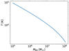 |
Fig. 3. TDE temperature dependent on BH mass using the L2 model. We assumed a solar-like star, that is, M⋆ = 1 M⊙ and R⋆ = 1 R⊙. |
As the emitting area is known for the temperature-dependent case, the flux can be directly computed from Eq. (7). The resulting flux is compared to the fixed-temperature L2 model in Fig. 4. For the temperature-independent models, the assumed temperature fixes the location of the BB peak, and the BH mass only acts as a multiplicative factor. In the temperature-dependent case, the BH mass enters into the flux through the emission area as a factor and additionally through the temperature in the emitted specific intensity. This means the location of the BB peak is determined by the BH mass. One consequence is that the bands are sensitive to different BH mass ranges because TDEs can be observed best when the BB peak is closely aligned with the observing band.
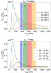 |
Fig. 4. Black body flux for different temperatures (upper panel) and BH masses (lower panel). For L2, T-indep. in the upper panel, |

2.3. Solving the rate integral
The rate integral in Eq. (1) only depends on two parameters at this point, the redshift and the BH mass, since we fixed the stellar mass and radius. These two parameters describe all possible TDEs we have considered. Similar to Szekerczes et al. (2024), we numerically integrated on a grid in this two-dimensional space but used a logarithmic grid spacing for the BH mass ranging from 105 M⊙ to 108 M⊙. We chose this BH mass region because on the lower end, the existence of intermediate-mass BHs is not yet confirmed (Davis et al. 2024; Pomeroy & Norris 2024). The upper end is chosen because for MBH ≳ 108 M⊙, stars would be swallowed whole (Hills 1975) as the tidal disruption radius becomes smaller than the event horizon. To obtain the correct integral region, we calculated the observed magnitude at each grid point and only kept those that produce a magnitude brighter than the observational limit. We used the magnitude limits for ZTF and LSST as a reference. For ZTF, the limits for the (g, r, i) band are (20.8, 20.6, 19.9), respectively (e.g., Bellm et al. 2019). For LSST, the limits for (u, g, r, i) are (23.3, 24.7, 24.3, 23.7), respectively (e.g., Huber et al. 2021; Lochner et al. 2022). The assumption that a TDE is observed at peak luminosity was introduced with the mass fallback rate in Eq. (11). We relaxed this assumption by subtracting 0.7 from the limiting magnitude of the survey in accordance with Szekerczes et al. (2024) and Oguri & Marshall (2010). It accounts for observations notcatching the TDE at its peak brightness but only close to it. The value of 0.7 gives a time window of tens of days to observe the TDE (e.g., Hinkle et al. 2020; Holoien et al. 2020). The limiting magnitudes of all surveys have this subtraction incorporated from this point onward.
3. Unlensed TDE rate
We show the results of our unlensed TDE rate calculations in Fig. 5. The vertical lines or bands represent the observational magnitude limit for ZTF and LSST. It is immediately apparent that the predictions of our considered models vary greatly. The spread easily exceeds a factor of 102 between the lowest and highest rates. This factor can climb above 103 in the i and u bands for bright limiting magnitudes ∼19. For faint limiting magnitudes ≳24, there seems to be a crossing region. Some models flatten out quicker, predicting a lower total TDE rate. This is mainly due to a smaller BHMF at a higher redshift; fewer BHs produce fewer TDEs.
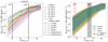 |
Fig. 5. Rate of TDEs as a function of survey limiting magnitude. The left panel shows the detection rate in the g band for the 33 models individually. We separated the color and line style information to keep the legend short. The right panel shows the detection rate in the u, r, and i bands, where each shaded region encompasses the spread in the models. We chose L2, TRINITY, 20 000 K as a fiducial model to guide the eye. The 33 models we considered for the unlensed TDE rate show a scattering factor of 𝒪(102) that can reach above 𝒪(103) for the u and i bands. The vertical black lines (left panel) and the colorful strips (right panel) show the observational magnitude limit for ZTF (g, r, i bands) and LSST (u, g, r, i bands). |
We tabulated the range of predictions for ZTF and LSST in Table 1. Independent of the TDE model, the g band observes the highest TDE rate for ZTF and LSST. In large part, this is due to both observatories having the faintest magnitude limit in the g band.
Predicted range of unlensed TDE rates.
In the following, we investigate the impact of the BHMF, the luminosity model, and the temperature individually. We find that the assumed temperature is responsible for most of the observed scatter between the different models.
3.1. Impact of black hole mass function
First, we chose the L2 model and fixed the temperature to 20 000 K. We only varied the BHMF (see Fig. 6). The unlensed TDE rate we calculated is very similar for the TRINITY and the COSMOS2015 BHMFs up to a magnitude limit of 25. This is clear when comparing the two BHMFs in Fig. 1. The two are almost identical for z ≲ 2, where most detectable TDEs are distributed (see Fig. E.1 for LSST limiting magnitudes). In contrast, the redshift independent model predicts lower rates by a factor of roughly four, which is due to the BHMF having a lower value at low redshift by roughly this factor of four.
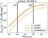 |
Fig. 6. Rate of TDEs as a function of survey limiting magnitude. Only the local BHMF impacts the unlensed TDE rates observed by current and near-future surveys such as ZTF and LSST. The redshift evolution of the BHMF influences the rate from a limiting magnitude of 25 onward. We have taken a representative subset from the left panel of Fig. 5 to clearly show the influence of the BHMF. |
The BHMFs strongly differ at large redshifts, which we can also observe in the predicted rates. They diverge for faint magnitude limits above around 25 (see Fig. 6). As the TRINITY BHMF decreases at high redshifts, the predicted TDE rates flatten out, while for the other two, only a slower increase is observed. This slowdown is attributed to the dimming of TDEs due to distance. At some point, even the brightest TDE are too far away to reach the magnitude limit. Overall, this implies that the redshift evolution of the BHMF only becomes important for faint magnitude limits above 25. These limits will not be reached by LSST, even when omitting the 0.7 reduction of the magnitude limit. However, redder bands detect the redshift evolution at a brighter magnitude than bluer bands. Red bands are naturally better suited to observe objects at high redshift. Hence, for a given magnitude limit, the highest redshift TDE always appears in the i band, allowing it to probe the redshift evolution of the BHMF at a brighter limiting magnitude than, for example, the u band. However, the temperature-dependent model can adjust for the alignment of the BB peak and the observing band. This adjustment changes the height of the BB peak by a factor of 𝒪(1). Hence, through the relation mAB ∝ log10(Fλ) (see Eq. (6)), the magnitude only changes by an additive constant ≃0. Thus, all bands detect the redshift evolution of the BHMF at the same limiting magnitude for the temperature-dependent models.
These results hint at a similar conclusion for the TDE rate per galaxy, as the BHMF and the TDE occurrence rate per galaxy influence the rate integral in the same way (see Eq. (1)). We find that the TDE rate per galaxy only plays a minor role. However, the different occurrence rate can impact the BH mass distribution, and through that, the cumulative TDE rate. But this change is small compared to other factors such as the assumed TDE temperature (see Sect. 3.3). We present the results of choosing the TDE occurrence rate from Chang et al. (2025) in Appendix B.
3.2. Impact of luminosity model
To investigate the impact of the luminosity model, we fixed the TRINITY BHMF and let the luminosity function vary (see Fig. 7). The two fixed-temperature luminosity models do not differ strongly in their unlensed TDE rate predictions. The L2 produces higher rates across almost all limiting magnitudes in all bands than L1. No matter the BHMF, the integrand of the rate integral (see Eq. (1)) has a small but negative dependence on the BH mass. Therefore, TDEs with a lower BH mass are preferred, which are brighter for L2 compared to L1. This trend holds until around a magnitude limit of 27, where both rates meet. The L2 flattens out more quickly than L1. This is due to the higher maximal luminosity that L1 allows for (see Fig. 2). At a given magnitude limit, this fact implies that TDEs can be observed at larger redshift for L1, meaning the volume in which observable TDEs can take place is larger.
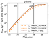 |
Fig. 7. Rate of TDEs as a function of survey limiting magnitude for different luminosity models. The luminosity model has little impact on the unlensed TDE rate. It can introduce a dependence of the rate on the observing band for the fixed-temperature models. The temperature-dependent model can compensate for the chosen observing band by selecting the TDE temperature. Thus, it does not show a strong band dependence. We have taken a representative subset from the left panel of Fig. 5 to clearly show the influence of the luminosity model. |
For the temperature-dependent model, the peak luminosity is higher than that for the fixed temperature L2 model. However, TDEs with high BH masses are suppressed with a lower luminosity. These two effects cancel each other such that almost the same rate of TDEs is observed for the temperature-dependent and the temperature-independent case.
3.3. Impact of temperature
The assumed temperature contributes the most to the spread of the models (see Fig. 8). The temperature strongly impacts the redshift distribution of the observed TDEs. As explained above, it is crucial that the peak of the BB spectrum aligns well with the observing band. At low redshift, the closest alignment is seen for 10 000 K; hence, models with this temperature show the highest rates at bright limiting magnitudes ≲22. The BB peak is always shifted into a given observing band at some redshift. Therefore, when a faint limiting magnitude ≳26 is assumed, all bands should roughly observe the same number of TDEs, as every TDE can be observed in every band. This is exactly what can be observed in Fig. 8. The odd one out is the 10 000 K model, as it does not quite reach the same level as the other temperatures. The same deviation is more prominent in the u band but not seen in the r or i bands. For this temperature, the peak of the BB spectrum lies at 290 nm at z = 0, which is just at a smaller wavelength compared to the u band. But the integrand in the numerator of the magnitude is proportional to λ ⋅ Fλobs (see Eq. (6)), meaning longer wavelengths are weighted more. With increasing redshift, the steep rise of the BB spectrum with increasing wavelength quickly dims the TDEs, as the peak of the BB shifts out of the u band and even the g band to longerwavelengths. For higher temperatures, the peak of the BB spectrum is first shifted into the observing band, counteracting the dimming due to distance. Therefore, TDEs are only observed at fainter magnitudes for 10 000 K, contributing to this model’s shallower slope. Hence, it takes longer to catch up to the models.
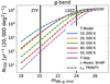 |
Fig. 8. Rate of TDEs as a function of survey limiting magnitude. The chosen temperature has the largest impact on the unlensed TDE rate. This parameter accounts for most of the scatter observed between the different models. This implies that it is crucial that the BB peak and the observing band are well aligned. We have taken a representative subset from the left panel of Fig. 5 to clearly show the influence of the temperature. |
3.4. Comparison to the observed rate
Hammerstein et al. (2023) report that ZTF observed 30 TDEs in 2.6 years in multi-band observations using g and r bands. ZTF observed the entire visible northern sky, roughly speaking around 20 000 deg2. This means they found an unlensed TDE rate NTDE of around 10 to 15 yr−1 (20 000 deg2)−1. In the g band, this rate is below all of our models. The lowest prediction is 16.5 yr−1 (20 000 deg2)−1, and it is from the L1z-independent 50 000 K model. For the r band, the rate lies between the L1 40 000 K and L2 50 000 K models, both for the redshift-independent BHMF.
Hammerstein et al. (2023) also inferred the temperature and found a range of around 15 000 K to 35 000 K with an average of 20 783 K. For this temperature range, our models would predict 108 (L1, z-indep., 30 000 K) to 2313 yr−1 (20 000 deg2)−1 (L2, COSMOS2015, 20 000 K) in the g band and 49.5 (L1, z-indep., 30 000 K) to 1538 yr−1 (20 000 deg2)−1 (L2, TRINITY, T-dep.) in the r band. In our calculation, we have not accounted for the effective year length of ZTF, which might lead to more incomplete observations than our models predict. We have also not accounted for other observational constraints, such as dust extinction or the host galaxy’s light. The implicit assumption is that a TDE is always observable. In practice, some TDE go undetected because of the bright host galaxy. In addition, we have also not accounted for completeness. The identification of TDEs is an active field of research (e.g., Zabludoff et al. 2021; Gomez et al. 2023; Stein et al. 2024). On top of that, removing the assumptions that every star is solar-like and every TDE is a full disruption could notably change the results. In general, lighter stars produce fainter TDEs, while heavier stars produce brighter TDEs. Hence, it is probable that the rate of detectable TDEs in magnitude-limited transient surveys may be lower when a realistic stellar mass distribution favors lower-mass stars. Whether these effects can account for a factor of 102 or can only explain part of the overestimation needs further analysis.
The inferred BH mass also yields little insight. Hammerstein et al. (2023) inferred a range between 106 M⊙ and 107 M⊙ using TDEmass (Ryu et al. 2020a) and a range from 2 · 106 M⊙ to 4 · 107 M⊙ using MOSFiT (Guillochon et al. 2018; Mockler et al. 2019). These BH mass distributions peak around the same mass as the L1 and the temperature-dependent L2 models, respectively. But as the BH mass is observationally not well constrained, we cannot establish a TDE luminosity model here. Nevertheless, this may indicate the possibility of inferring the TDE luminosity model using the BH mass distribution. This is especially feasible when better statistics become available with the launch of LSST. However, the BH mass must be measured robustly for such an investigation.
4. Lensed TDE rate
In this section, we outline our methods to calculate the lensed TDE rate and show our results. In Fig. 9 we show an illustration of a lensed TDE with two images of the TDE. We refer to such a lensing event as a doubly lensed TDE or simply as a double. For more details on gravitational lensing, we refer to Appendix C.
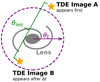 |
Fig. 9. Illustration of a lensed TDE with two images, A and B, around a galaxy acting as a lens. The lens has an Einstein radius, θE, that gives an estimate of the image separation, θsep. Due to the different geometric path lengths and the gravitational time delay (Shapiro 1964), we expect image B to appear later than image A with a time delay of Δt. |
4.1. Calculating the lensed rates
The lensed TDE rate is calculated with the code developed by Oguri & Marshall (2010). Some optimizations have been introduced to the code to speed up calculation times significantly. For details, we refer to Appendix D. For the calculations, the code from Oguri & Marshall (2010) assumes that all lens galaxies are singular isothermal ellipsoids with convergence
 (19)
(19)
where λ(e) is the dynamical normalization, e is the ellipticity, and
 (20)
(20)
is the Einstein radius, which is dependent on the velocity dispersion, v, of the lens galaxy and the angular diameter distance from the observer to the source, Ds, and from the lens to the source, Dds. This is an elliptical profile, which implies that the Einstein radius gives an estimate of the separation of the different images. The lens model is singular and isothermal, meaning the mass distribution drops as 1/r and diverges at the origin. These equations and the corresponding deflection of light rays for the singular isothermal ellipsoid were derived by Kormann et al. (1994).
The code calculates a lensed TDE mock catalog by taking in an unlensed mock catalog and simulating all possible lens galaxies as elliptical galaxies, which make up ∼80% of the lensing probability (Turner et al. 1984; Fukugita et al. 1992; Kochanek 1996; Chae 2003; Oguri 2006; Möller et al. 2007). Hence, every lens can be described by its redshift and velocity dispersion in a two-dimensional parameter space. The same technique for generating a mock catalog of unlensed TDEs can be used to create a catalog of possible lens galaxies. By estimating an area on the sky larger than any possible lens system, the lensing code by Oguri & Marshall (2010) can calculate a rate of finding a TDE in the vicinity of a lens galaxy, assuming both lenses and TDEs are spread uniformly on the survey area. This assumption is equivalent to the isotropy of the Universe (e.g., Goodman 1995; Clarkson & Maartens 2010; Kumar Aluri et al. 2023; Bengaly et al. 2024). By sampling a Poisson distribution with the close separation rate estimate, they can find the number of candidate systems. The lens equation is then solved for these systems to determine whether it is an actual lens or just a close separation with no multiple images. All systems that produce multiple images are then saved to a mock catalog. A TDE lensed into a double is considered observable when both images are brighter than the limiting magnitude. A schematic diagram of a doubly lensed TDE is shown in Fig. 9. The third brightest image must be brighter than the magnitude limit for a quad lensed TDE. Calculating rates from such a mock catalog is as simple as counting the entries brighter than the magnitude limit. However, to calculate rates smaller than 1 yr−1 (20 000 deg2)−1, we need to oversample. We achieved this by calculating N catalogs and, in the end, dividing the summed number of systems by N. Thus, every entry in a mock catalog only counts as 1/N toward the rate. This mock catalog counting suffers from Poisson noise, so the error scales with  .
.
Predicted range of lensed TDE rates.
4.2. Lensed rate results
Following Szekerczes et al. (2024), we only selected lensed events with an image separation in the range [0.5″, 4″] to ensure that the multiple images can be resolved by ground-based surveys such as LSST. For a quad, we measured the maximal distance between two images. We included all images of a quad. In a cusp configuration, the fourth image typically sets the largest image separation, but it is also demagnified. However, deeper imaging can reveal it, and we considered the system resolvable. We only considered the lensed rate for LSST limiting magnitudes. We did not examine ZTF limits because many models predict a smaller rate than our numerical limit of 10−3 yr−1 (20 000 deg2)−1, with an oversampling factor of 1000.
The lensed rates show, just like the unlensed ones, a large scatter of 𝒪(102) in the four bands (see Fig. 10). The overall trend is similar to the unlensed rates. Initially, the rate increases steeply and flattens toward fainter limiting magnitudes around 25 or 26. For LSST, we tabulated the range of predictions in Table 2. Just as for the unlensed rates, only the local BHMF is important for the rate prediction. The redshift evolution of the BHMF only impacts the rate for magnitude limits fainter than those reached by LSST. The lensed rate shows the influence of the redshift evolution at a brighter limiting magnitude of 24 than the unlensed rate because the magnification due to lensing allows TDEs to be observed at a greater distance from us. The main contribution to the scattering of the different models still stems from the assumed temperature. Just as in the unlensed case, the luminosity model has little impact on the lensed TDE rate.
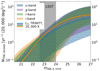 |
Fig. 10. Rates of lensed TDEs as a function of survey limiting magnitude. The lensed TDE rates also show a scattering factor of 𝒪(102) that can almost reach 𝒪(103). The gray strip shows the observational magnitude limit for LSST (u, g, r, i bands). We display L2, TRINITY, 20 000 K as a fiducial model in solid lines to guide the eye. |
4.3. Lensed fraction
The unlensed and lensed TDE rate predictions both exhibit a broad spread. Therefore, we further investigated the lensed fraction to estimate the fraction of observed TDE that are part of a lensing system. We present in Fig. 11 the lensed fractions for LSST magnitude limits. In the plot, each point or line indicates the ratio of observable lensed TDEs to observable unlensed TDE given a LSST magnitude limit. The horizontal lines are used for the temperature-dependent L2 models, which cover a wide range of possible TDE temperatures. The lensed fraction is more robust against the different model parameters and displays a smaller scattering factor of ∼50 between the lowest and highest fractions. We predict the fraction of lensed to unlensed TDEs to be between 1.7 ⋅ 10−5 (L1, TRINITY, 10 000 K, u band) and 8.7 ⋅ 10−4 (L1, z-indep., 50 000 K, g band). As an order of magnitude, we can say that in order to observe one lensed TDE, LSST has to observe thousands to tens of thousands of unlensed TDEs.
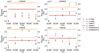 |
Fig. 11. Lensed fraction for the different TDE models. Each point represents the fraction of TDEs observed as part of a lensing system. The lines are used for the temperature-dependent L2 models. The fractions of lensed TDEs show a greatly reduced scatter than the scatter of the unlensed and lensed rates. The fractions lie within a factor of 50. We calculated these lensed fractions for the LSST magnitude limits. |
The lensed TDE population includes many TDEs at a higher redshift than found in the unlensed population. Thus, a larger lensed fraction implies that the fading of TDEs is more strongly counteracted, either due to an increasing BHMF with redshift or due to a better BB peak alignment. Overall, we can interpret the lensed fraction as a value that compares the number of observable TDEs at low and high redshifts. This becomes clearer when comparing the first row of Fig. 12 to the first row of Fig. E.1. The lensed TDEs have a median redshift between 2 and 3, while the unlensed TDEs have a median redshift between 0.2 and 0.7.
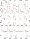 |
Fig. 12. Differential rate of lensed TDEs for five representative models. The rows from top to bottom are the TDE redshifts, BH masses, lens redshifts, lens velocity dispersions, lensed image separations, and time delays of doubles. The three time delays for quads are shown in Appendix F. These figures were calculated for LSST magnitude limits. |
To better understand Fig. 11, we considered the observing bands individually. In the u band, we observed the smallest lensed fractions. Here, we know that a temperature of 10 000 K aligns the BB peak well with the u band at low redshifts, but this alignment is broken at larger redshifts, and only a few TDEs are observed. Thus, we find a small lensed fraction. The fraction increases with temperature because the low redshift alignment of the BB peak gets worse, while the alignment gets better for a larger redshift. We expect most lensed TDEs to be around z = 1 (see the first row of Fig. 12). At this redshift, a temperature between 20 000 K and 30 000 K is best aligned with the u band. Hence, we do not expect the increasing trend of the lensed fraction to continue much beyond this temperature. The temperature-dependent models can compensate for the BB peak alignment and reach higher temperatures and redshifts. Therefore, they predict many TDEs at low redshift. But with the possibility of very high temperatures, they produce many observable TDEs in the u band at a high redshift. Thus, temperature-dependent models yield the highest fraction in the u band.
We observed the same trend of the lensed fraction in the g band (see the upper right panel of Fig. 11). But the rise of the fraction continues up to 50 000 K. This is due to the possibility of observing lensed TDEs up to z ≲ 4 in the g band, while unlensed TDEs fade from view at z ≳ 0.7.
In the r and i bands, the peak of the lensed fraction moves to lower temperatures because these temperatures perform best in the respective bands at high redshifts. It is worth noting that in the i band at 50 000 K, we find the lowest lensed fraction despite the fact that the i band observes very few unlensed TDEs at this temperature. However, the i band lies too far away from the BB peak. Hence, the dimming due to distance fades any lensed TDE from view long before the BB peak can be aligned with the band. Therefore, the i band does not observe many lensed TDEs either, indicating a small lensed fraction.
The different BHMFs seem to amplify the influence of the temperature. Comparing the two redshift-dependent BHMFs, we observed that the COSMOS2015 BHMF increases the fraction compared to the TRINITY BHMF only for the temperature-dependent model. This is because the temperature-dependent model reaches the highest redshift (see the first row of Fig. 12). Therefore, the redshift evolution can no longer be neglected, and the increase of the COSMOS2015 BHMF for low-mass BHs does matter. The redshift-independent BHMF amplifies the influence of the temperature the most. This makes sense, as a decreasing BHMF with redshift always leads to a decrease in TDEs observed at high redshift. The redshift-independent BHMF does not show any evolution and can therefore more easily produce high TDE rates at high redshift.
4.4. Lensing parameters
Lastly, we investigated the different parameters of the lensed TDE population. We selected a subset of five models to allow each parameter or combination of parameters to be varied. The distributions shown are for LSST limiting magnitudes in Fig. 12.
First, we considered the TDE parameters: source redshift and BH mass (see the first and second rows of Fig. 12), respectively. We expected most lensed TDEs to be observed between redshift 1 and 2. Overall, the g band is always best suited to observe TDEs because it has the faintest limiting magnitude. As expected, the BH mass distribution follows the shape of the magnitude functions. The brighter TDEs at a given BH mass, the more of these TDEs are observed.
Second, we assessed the lens parameters, which are the lens redshift and lens velocity dispersion (see the third and fourth rows of Fig. 12, respectively). As expected, the TDE model has little to no effect on the lenses. For the temperature-dependent and the 40 000 K models, we observed lenses at a higher redshift, but this is solely due to the fact that in these models, TDEs can also be observed at a larger redshift. Most lenses sit at z ≲ 1 and have a velocity dispersion between 100 and 300 km s−1.
Third, we examined the parameters of the resulting lens system. The image separation is shown in the fifth row and the time delay of doubles is shown in the sixth row of Fig. 12. Additionally, we tabulated the ratio of double to quad lenses in Table 3. For quads, the maximal image separation was taken. These parameters are also largely independent of the chosen TDE model. Only the fact that some models predict TDEs at higher redshifts influences the distributions. Most images have an image separation below 3″, but the smaller the image separation, the more probable such a system is. As mentioned earlier, the image separation was cut at 0.5″. Similarly independent is the time delay of doubles. Most lens systems display a time delay ranging from a few days to around 100 days. Models that predict TDEs at higher redshifts also observe longer time delays. Quads show a very similar time-delay distribution for the longest time delay. The second and third time-delay distributions are shifted to shorter time delays. Their peak is around 4 days instead of around 11 days. Their distributions are shown in Appendix F.
Rate of double and quad lensed TDEs, the ratio of double to quad lenses, and the fraction of quad to total lenses.
Our analysis suggests around three or four doubles for one quad system. In Table 3, the ratio of doubles to quads falls into a range from 0.96 to 5.41. Here, the maximal redshift of the different TDE models plays a large role in the ratio of doubles to quads. Doubles typically prefer lower redshifts, while quads prefer higher redshifts. The exemplary L2, COSMOS2015, 20 000 K model clearly shows that the quad lenses peak around redshift 2, while the double lenses peak approximately at z = 1 in the g, r and i bands. For the u band, quads also peak at a higher redshift than doubles. This difference in the preferred redshift is due to the fact that the tangential caustic typically provides a higher magnification than the radial caustic (Venumadhav et al. 2017; Meena et al. 2022). Therefore, quads are more likely to receive a large boost in brightness and are more likely to be observed at great distances. If a given TDE model predicts more lensed TDEs at low redshifts compared to another model, we expect the former one to display a larger ratio. In Table 3, we also calculate the fraction of quad lenses relative to the total number of lensed TDEs. We find that between 16 to 39% of lensed TDEs will be a quad system. Oguri & Marshall (2010) predict in their catalogs for LSST that 13% of lensed quasars and 30 to 32% of lensed supernovae will be observed as quad lenses. Hence, our results are comparable to their findings.
5. Conclusion
In this paper, we have numerically calculated the predicted unlensed and lensed TDE rate as a function of limiting magnitude in four bands. We covered the ongoing ZTF and the future LSST surveys and different model parameters such as the BHMF, TDE luminosity model, and assumed flare temperature. For the unlensed rates, our models predict between 16 and 5440 yr−1 (20 000 deg2)−1 for ZTF in the g band. For LSST, the rate is in the range from 3580 to 82 060 yr−1 (20 000 deg2)−1. In both surveys, the g band stands out as the best option to observe TDEs because it has the faintest limiting magnitude. The sizable scattering factor of 𝒪(102) up to ∼103 that the models display can be attributed to the assumed TDE temperature, making it the most critical assumption for TDE rate estimates. Despite the uncertain predictions, we have demonstrated that only the local BHMF is relevant for current and near-future surveys. Our redshift-dependent BHMF only showed a significant deviation from the redshift-independent model at a limiting magnitude of 25 or fainter. As LSST will only reach about magnitude 24, the redshift evolution of the BHMF is not important to LSST. Compared to the observational unlensed TDE rate around 10 to 15 yr−1 (20 000 deg2)−1 obtained from ZTF, most of our models overestimate the rate. It should be expected that we overestimate the observed rate, as we have not accounted for completeness or any observational effects in our calculations. For a more accurate estimate in the future, we could include the host galaxy light or dust extinction to better match observations. Furthermore, removing the assumption that every star is solar-like would yield even more accurate results. Last, certain physical processes in TDEs can also make the detected TDE rates significantly deviate from the theoretical rates (Wong et al. 2022).
From our investigation into the lensed fraction, we can approximate that for every 10 000 unlensed TDEs, we expect LSST to find a few lensed events. The results show a reduced scatter to around a factor of 50. As our unlensed rates only poorly match observational ones, it seems improbable that a large sample of hundreds of lensed TDE can be obtained. Yet, LSST will observe a few lensed TDEs over its 10-year survey time. Lensed TDEs are also best observed in the g band due to its faint limiting magnitude. For LSST, our predictions range from one every two years to more than ten yearly, assuming 20 000 deg2 in the g band, still showing much of the scatter also observed for the unlensed rate. However, analogously to the unlensed rate, we were able to show that the TDE temperature is the most important assumption and only the BHMF is relevant even beyond LSST limiting magnitudes.
Ryu et al. (2020a) include a correction factor to account for the uncertainty in the relation between the elliptical emission area and the black body radius. However, for simplicity, we followed Ryu et al. (2020a) in assuming they are comparable.
Acknowledgments
We thank Volker Springel for the helpful discussion on BHMFs. EM and SHS thank the Max Planck Society for support through the Max Planck Fellowship for SHS. KS acknowledges support through a Fulbright grant of the German-American Fulbright Commission. LD acknowledges the support from the Hong Kong Research Grants Council (17304821, 17314822, 17305124). This work was supported by JSPS KAKENHI Grant Numbers JP23K22531, JP22K21349, JP19KK0076.
References
- Baehr, H. D., & Kabelac, S. 2016, Thermodynamik (Springer) [Google Scholar]
- Bellm, E. C., Kulkarni, S. R., Graham, M. J., et al. 2019, PASP, 131, 018002 [Google Scholar]
- Bengaly, C. A. P., Alcaniz, J. S., & Pigozzo, C. 2024, Phys. Rev. D, 109, 123533 [CrossRef] [Google Scholar]
- Bessell, M., & Murphy, S. 2012, PASP, 124, 140 [NASA ADS] [CrossRef] [Google Scholar]
- Bricman, K., & Gomboc, A. 2020, ApJ, 890, 73 [NASA ADS] [CrossRef] [Google Scholar]
- Chae, K.-H. 2003, MNRAS, 346, 746 [NASA ADS] [CrossRef] [Google Scholar]
- Chang, J. N. Y., Dai, L., Pfister, H., Kar Chowdhury, R., & Natarajan, P. 2025, ApJ, 980, L22 [Google Scholar]
- Chen, Z., Lu, Y., & Chen, Y. 2024, ApJ, 962, 3 [NASA ADS] [CrossRef] [Google Scholar]
- Cheng, T.-P. 2005, Relativity, Gravitation and Cosmology. A Basic Introduction (Oxford University Press) [Google Scholar]
- Clarkson, C., & Maartens, R. 2010, Class. Quant. Grav., 27, 124008 [Google Scholar]
- Davidzon, I., Ilbert, O., Laigle, C., et al. 2017, A&A, 605, A70 [NASA ADS] [CrossRef] [EDP Sciences] [Google Scholar]
- Davis, B. L., Graham, A. W., Soria, R., et al. 2024, ApJ, 971, 123 [Google Scholar]
- Fukugita, M., Futamase, T., Kasai, M., & Turner, E. L. 1992, ApJ, 393, 3 [Google Scholar]
- Gallo, E., & Sesana, A. 2019, ApJ, 883, L18 [NASA ADS] [CrossRef] [Google Scholar]
- Gezari, S. 2013, American Astronomical Society Meeting Abstracts, 221, 131.02 [Google Scholar]
- Gezari, S. 2021, ARA&A, 59, 21 [NASA ADS] [CrossRef] [Google Scholar]
- Gezari, S., Heckman, T., Cenko, S. B., et al. 2009, ApJ, 698, 1367 [Google Scholar]
- Gomez, S., Villar, V. A., Berger, E., et al. 2023, ApJ, 949, 113 [Google Scholar]
- Goodman, J. 1995, Phys. Rev. D, 52, 1821 [Google Scholar]
- Guillochon, J., Nicholl, M., Villar, V. A., et al. 2018, ApJS, 236, 6 [NASA ADS] [CrossRef] [Google Scholar]
- Hammerstein, E., van Velzen, S., Gezari, S., et al. 2023, ApJ, 942, 9 [NASA ADS] [CrossRef] [Google Scholar]
- Hills, J. G. 1975, Nature, 254, 295 [Google Scholar]
- Hills, J. G. 1988, Nature, 331, 687 [Google Scholar]
- Hinkle, J. T., Holoien, T. W. S., Shappee, B. J., et al. 2020, ApJ, 894, L10 [NASA ADS] [CrossRef] [Google Scholar]
- Holoien, T. W. S., Auchettl, K., Tucker, M. A., et al. 2020, ApJ, 898, 161 [NASA ADS] [CrossRef] [Google Scholar]
- Huber, S., Suyu, S., Noebauer, U. M., et al. 2021, A&A, 646, A110 [NASA ADS] [CrossRef] [EDP Sciences] [Google Scholar]
- Ivezić, Ž., Kahn, S. M., Tyson, J. A., et al. 2019, ApJ, 873, 111 [Google Scholar]
- Kochanek, C. S. 1996, ApJ, 466, 638 [Google Scholar]
- Kochanek, C. S. 2004, ApJ, 605, 58 [Google Scholar]
- Komossa, S., Halpern, J., Schartel, N., et al. 2004, ApJ, 603, L17 [NASA ADS] [CrossRef] [Google Scholar]
- Kormann, R., Schneider, P., & Bartelmann, M. 1994, A&A, 284, 285 [NASA ADS] [Google Scholar]
- Kormendy, J., & Ho, L. C. 2013, ARA&A, 51, 511 [Google Scholar]
- Kumar Aluri, P., Cea, P., Chingangbam, P., et al. 2023, Class. Quant. Grav., 40, 094001 [NASA ADS] [CrossRef] [Google Scholar]
- Laigle, C., McCracken, H. J., Ilbert, O., et al. 2016, ApJS, 224, 24 [Google Scholar]
- Lin, D., Guillochon, J., Komossa, S., et al. 2017, New Astron., 1, 0033 [Google Scholar]
- Lin, Z., Jiang, N., & Kong, X. 2022, MNRAS, 513, 2422 [Google Scholar]
- Lochner, M., Scolnic, D., Almoubayyed, H., et al. 2022, ApJS, 259, 58 [NASA ADS] [CrossRef] [Google Scholar]
- Meena, A. K., Arad, O., & Zitrin, A. 2022, MNRAS, 514, 2545 [CrossRef] [Google Scholar]
- Meneghetti, M. 2021, Introduction to Gravitational Lensing: With Python Examples (Springer Cham) [Google Scholar]
- Mockler, B., Guillochon, J., & Ramirez-Ruiz, E. 2019, ApJ, 872, 151 [Google Scholar]
- Möller, O., Kitzbichler, M., & Natarajan, P. 2007, MNRAS, 379, 1195 [Google Scholar]
- Oguri, M. 2006, MNRAS, 367, 1241 [NASA ADS] [CrossRef] [Google Scholar]
- Oguri, M., & Marshall, P. J. 2010, MNRAS, 405, 2579 [NASA ADS] [Google Scholar]
- Pfister, H., Volonteri, M., Dai, L., & Colpi, M. 2020, MNRAS, 497, 2276 [NASA ADS] [CrossRef] [Google Scholar]
- Pfister, H., Toscani, M., Wong, T. H. T., et al. 2022, MNRAS, 510, 2025 [Google Scholar]
- Piran, T., Svirski, G., Krolik, J., Cheng, R. M., & Shiokawa, H. 2015, ApJ, 806, 164 [Google Scholar]
- Planck, M. 1901, Ann. Phys., 309, 553 [NASA ADS] [CrossRef] [Google Scholar]
- Pomeroy, R. T., & Norris, M. A. 2024, MNRAS, 530, 3043 [Google Scholar]
- Rauch, K. P., & Blandford, R. D. 1991, ApJ, 381, L39 [NASA ADS] [CrossRef] [Google Scholar]
- Rees, M. J. 1988, Nature, 333, 523 [Google Scholar]
- Refsdal, S. 1964, MNRAS, 128, 307 [NASA ADS] [CrossRef] [Google Scholar]
- Reusch, S., Stein, R., Kowalski, M., et al. 2022, Phys. Rev. Lett., 128, 221101 [NASA ADS] [CrossRef] [Google Scholar]
- Rybicki, G. B., & Lightman, A. P. 1979, Radiative Processes in Astrophysics (John Wiley& Sons) [Google Scholar]
- Ryu, T., Krolik, J., & Piran, T. 2020a, ApJ, 904, 73 [NASA ADS] [CrossRef] [Google Scholar]
- Ryu, T., Krolik, J., Piran, T., & Noble, S. C. 2020b, ApJ, 904, 98 [NASA ADS] [CrossRef] [Google Scholar]
- Schneider, P., Ehlers, J., & Falco, E. E. 1992, Gravitational Lenses (Berlin, Heidelberg: Springer) [Google Scholar]
- Schneider, P., Kochanek, C., & Wambsganss, J. 2006, Gravitational Lensing: Strong, Weak and Micro, Saas-Fee Advanced Course (Berlin, Heidelberg: Springer) [Google Scholar]
- Shapiro, I. I. 1964, Phys. Rev. Lett., 13, 789 [Google Scholar]
- Shimizu, T., Oogi, T., Okamoto, T., Nagashima, M., & Enoki, M. 2024, MNRAS, 531, 851 [Google Scholar]
- Stein, R., Mahabal, A., Reusch, S., et al. 2024, ApJ, 965, L14 [Google Scholar]
- Szekerczes, K., Ryu, T., Suyu, S. H., et al. 2024, A&A, 690, A384 [NASA ADS] [CrossRef] [EDP Sciences] [Google Scholar]
- Thomsen, L. L., Kwan, T. M., Dai, L., et al. 2022, ApJ, 937, L28 [NASA ADS] [CrossRef] [Google Scholar]
- Toscani, M., Rossi, E. M., & Lodato, G. 2020, MNRAS, 498, 507 [Google Scholar]
- Toscani, M., Rossi, E. M., Tamanini, N., & Cusin, G. 2023, MNRAS, 523, 3863 [Google Scholar]
- Turner, E. L., Ostriker, J. P., & Gott, J. R., III 1984, ApJ, 284, 1 [NASA ADS] [CrossRef] [Google Scholar]
- Venumadhav, T., Dai, L., & Miralda-Escudé, J. 2017, ApJ, 850, 49 [NASA ADS] [CrossRef] [Google Scholar]
- Wevers, T., & Ryu, T. 2023, arXiv e-prints [arXiv:2310.16879] [Google Scholar]
- Wong, T. H. T., Pfister, H., & Dai, L. 2022, ApJ, 927, L19 [NASA ADS] [CrossRef] [Google Scholar]
- Wozniak, P. R., Graham, M. J., Mahabal, A. A., & Seaman, R., eds. 2014, The Third Hot-wiring the Transient Universe Workshop (HTU-III) [Google Scholar]
- Yonehara, A., Mineshige, S., Fukue, J., Umemura, M., & Turner, E. L. 1999, A&A, 343, 41 [NASA ADS] [Google Scholar]
- Zabludoff, A., Arcavi, I., LaMassa, S., et al. 2021, Space Sci. Rev., 217, 54 [NASA ADS] [CrossRef] [Google Scholar]
- Zhang, H., Behroozi, P., Volonteri, M., et al. 2023, MNRAS, 518, 2123 [Google Scholar]
Appendix A: Magnitude integral
To calculate the flux integral in the numerator of Eq. 6, we first introduced the variables a and b to simplify calculations. The flux then takes the form
We obtained this expression by plugging Eq. 8 into Eq. 7. The integral could then be computed as follows:
![Mathematical equation: $$ \begin{aligned} \int _{0}^{\infty } \mathrm{d} \lambda \; \lambda \cdot S_{\mathrm{X} } \cdot F_{\lambda , \mathrm{o} }&= \int _{\lambda _{\mathrm{min} }}^{\lambda _{\mathrm{max} }} \mathrm{d} \lambda \; \lambda \cdot \frac{a}{\lambda ^{5}} \cdot \frac{1}{e^{\frac{b}{\lambda }} -1} = \\[5pt]&= a \int _{\lambda _{\mathrm{min} }}^{\lambda _{\mathrm{max} }} \mathrm{d} \lambda \; \frac{1}{\lambda ^{4}} \cdot \frac{1}{e^{\frac{b}{\lambda } -1}} = \\[5pt] \left[ \mathrm{Subs.} \; \frac{b}{\lambda } = x \right] \;\;\;&= a \int _{\frac{b}{\lambda _{\mathrm{min} }}}^{\frac{b}{\lambda _{\mathrm{max} }}} \mathrm{d} x \; \left( -\frac{b}{x^{2}} \right) \cdot \left( \frac{b}{x} \right)^{-4} \cdot \frac{1}{e^{x} -1} = \\[5pt]&= -\frac{a}{b^{3}} \int _{\frac{b}{\lambda _{\mathrm{min} }}}^{\frac{b}{\lambda _{\mathrm{max} }}} \mathrm{d} x \; \frac{x^{2}}{e^{x} -1}. \end{aligned} $$](/articles/aa/full_html/2025/09/aa54367-25/aa54367-25-eq28.gif)
To solve this integral, we first solved

by substituting u = 1 − e−x, from which follows
By re-substituting, we found
We could then solve the flux integral by applying partial integration (PI) twice:
![Mathematical equation: $$ \begin{aligned} \int \mathrm{d} x \; \frac{x^{2}}{e^{x} -1}&\mathop {=}\limits ^{\mathrm{PI} } \left[ x^{2} \cdot \ln (1 - e^{-x}) \right] - \int \mathrm{d} x \; 2x \ln (1 - e^{-x}) = \\[5pt]&= -x^{2} \cdot \mathrm{Li} _{1}(e^{-x}) + 2\int \mathrm{d} x \; x \mathrm{Li} _{1}(e^{-x}) = \\[5pt] \left[ \mathrm{Subs.} \; u = e^{-x} \right] \;\;\;&= -x^{2} \cdot \mathrm{Li} _{1}(e^{-x}) + 2\int \mathrm{d} u \; \frac{\ln (u)}{u} \mathrm{Li} _{1}(u) = \\[5pt]&\mathop {=}\limits ^{\mathrm{PI} } -x^{2} \cdot \mathrm{Li} _{1}(e^{-x}) + 2\left[ \ln (u) \cdot \mathrm{Li} _{2}(u) \right] \\&\quad - 2\int \mathrm{d} u \; \frac{1}{u} \mathrm{Li} _{2}(u) = \\[5pt]&= -x^{2} \cdot \mathrm{Li} _{1}(e^{-x}) + 2 \ln (u) \cdot \mathrm{Li} _{2}(u) \\[3pt]&\quad - 2\left[ \mathrm{Li} _{3}(u) \right] = \\[5pt] \left[ \mathrm{Re-subs.} \right] \;\;\;&= -x^{2} \cdot \mathrm{Li} _{1}(e^{-x}) - 2 x \cdot \mathrm{Li} _{2}(e^{-x}) - 2 \mathrm{Li} _{3}(e^{-x}), \end{aligned} $$](/articles/aa/full_html/2025/09/aa54367-25/aa54367-25-eq32.gif)
where  is the polylogarithm, with Li1(x) = − ln(1 − x). The final result could then be expressed as
![Mathematical equation: $$ \begin{aligned}&\int _{0}^{\infty } \mathrm{d} \lambda \; \lambda \cdot S_{\mathrm{X} } \cdot F_{\lambda , \mathrm{o} } = \\ &= \frac{a}{b^{3}} \left[ \left( \frac{b}{\lambda } \right)^{2} \cdot \mathrm{Li} _{1} \left( e^{-\frac{b}{\lambda }} \right) + 2 \frac{b}{\lambda } \cdot \mathrm{Li} _{2} \left( e^{-\frac{b}{\lambda }} \right) + 2 \mathrm{Li} _{3} \left( e^{-\frac{b}{\lambda }} \right) \right]^{\frac{b}{\lambda _{\mathrm{max} }}}_{\frac{b}{\lambda _{\mathrm{min} }}}. \end{aligned} $$](/articles/aa/full_html/2025/09/aa54367-25/aa54367-25-eq34.gif)
Appendix B: Impact of the TDE occurrence rate
In order to examine the impact of the TDE occurrence rate, we considered a different TDE rate per galaxy (Chang et al. 2025)
 (B.1)
(B.1)
Compared to the uniform power law from Pfister et al. (2020), this function peaks at MBH ≃ 106 M⊙ and covers a larger TDE occurrence rate range, due to the larger exponents of ±1.2. It peaks above the one from Pfister et al. (2020) but falls off more steeply toward smaller or larger BH masses. In Fig. B.1 we show the impact of the TDE occurrence rate on the cumulative, unlensed TDE rate. We have fixed the BHMF to the TRINITY model as a representative case. Overall, the impact of the TDE occurrence rate is small, especially when compared to the fixed temperature case. The impact of the TDE occurrence rate is mainly driven through the alteration of the BH mass distribution.
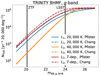 |
Fig. B.1. Impact of a different TDE occurrence rate per galaxy on the cumulative, unlensed TDE rate. The TDE occurrence rate mainly acts as a constant offset with an overall weak influence on the TDE rate. |
Fig. B.2 shows that the BH mass distribution reflects the TDE occurrence rate. The BH mass distribution with the occurrence rate by Chang et al. (2025) shows a peak around 106 M⊙ and drops off more steeply toward lower or higher bh masses. A change in BH mass distribution also means a difference in TDE luminosity distribution. This new BH mass distribution has more TDEs at ∼ 106 M⊙ where the L1 luminosity peaks. Hence, for the L1 model, more of these luminous TDEs are detected with a resulting increase in the number of observed TDEs shown in Fig. B.1. In contrast, a shift in the bh mass only changes the luminosity of the fixed temperature L2 model marginally. Hence, we do not observe a different cumulative TDE rate. In the temperature-dependent case, the luminosity decreases only slightly between 105 M⊙ and 106 M⊙, but falls off steeply toward higher BH masses. A lowering of the number of BHs at these higher BH masses (∼107 to 108 M⊙) would therefore only mildly decrease the number of TDEs, whereas the higher number of BHs at ∼106 M⊙ would increase the number of TDEs more significantly. Hence, the shift in BH mass distribution leads to an overall increase in the cumulative TDE rate, even if the most luminous TDEs are less abundant.
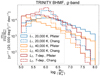 |
Fig. B.2. BH mass distribution for different TDE occurrence rates. These distributions are calculated for LSST magnitude limits. |
Appendix C: Gravitational lensing
For our calculations involving gravitational lensing, we use the code from Oguri & Marshall (2010). They follow a standard approach to gravitational lensing using the thin-lens approximation (e.g. Schneider et al. 1992, 2006; Cheng 2005; Meneghetti 2021). As the distances between the observer, lens, and source are much greater than the extent of the lens and the source, both the lens and the source are projected onto 2D planes, the lens and source plane, respectively. We show this basic setup in Fig. C.1. We can rescale the coordinates in the respective planes to angles measured by the observer using the distances DX. We denote the distances between the observer and the lens, the observer and the source, and the lens and the source with Dd, Ds, and Dds, respectively. As these distances are large, the small-angle approximation holds, meaning the angles can be treated as two-dimensional Euclidean coordinates. The governing equation, also known as the lens equation
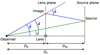 |
Fig. C.1. Schematic view of a gravitational lens. The light travels along the blue path, meaning we observe the image at a different angular position θ compared to the true angular source position β indicated with the green line. |
 (C.1)
(C.1)
can then be geometrically derived. Here, β is the true source position on the source plane, θ is the observed position of the lensed source on the lens plane, and  is the deflection angle of the light at the lens plane. By absorbing the distance fraction, the deflection angle is rescaled to the scaled deflection angle
 (C.2)
(C.2)
where  denotes the convergence, a dimensionless quantity, related to the projected mass density Σ. It is scaled to the critical mass density Σcrit = c2/(4πG)⋅Ds/(DdDds).
An important quantity in lensing is the magnification. The flux from a source is increased by this factor due to the light being focused by the lens. The magnification
![Mathematical equation: $$ \begin{aligned} \mu = \frac{1}{\det A_{ij}} = \left[ \det \left( \frac{\partial \beta _{i}}{\partial \theta _{j}} \right) \right]^{-1} \end{aligned} $$](/articles/aa/full_html/2025/09/aa54367-25/aa54367-25-eq40.gif) (C.3)
(C.3)
can be calculated using the Jacobian matrix Aij, which gives the distortion of the lensed images. The determinant can vanish, leading to an infinite magnification. The curves where this happens are called critical curves on the lens plane and caustics on the source plane. In practice, the magnifications of the lensed sources near critical curves are high yet finite because geometric optics (thin-lens approximation) is no longer applicable in this regime, and wave optics is needed.
Appendix D: Implementation
In the original implementation from Oguri & Marshall (2010), all possible lens galaxies are described by two parameters, the redshift and velocity dispersion. Hence, the code calculates through a two dimensional grid. At each grid point, the number of galaxies is calculated, and for every lens galaxy, the number of possible TDEs is drawn from a Poisson distribution. As an example, when considering 20, 000 deg2 on the sky, we calculate above 358 billion galaxies up to a redshift of 2. Drawing 1 billion samples from a Poisson distribution takes on the order of one minute, which means a lot of time is spent on this portion of the code.
As all lens galaxies are considered the same at a given grid point, we only need to calculate the total number of possible TDEs for N galaxies. Here we can use the fact that the sum of two independent Poisson distributed variables is also Poisson distributed. When X ∼ Poisson(λ) and Y ∼ Poisson(μ) then X + Y ∼ Poisson(λ + μ). Therefore, we do not need to draw N times from a Poisson distribution with expectation value λ but we can draw from a Poisson distribution with N ⋅ λ as its expectation value a single time, significantly speeding up calculations.
Other optimizations have been made by removing the need to instantiate large data arrays not needed for this application of the code, yielding significant performance improvement without changing the code’s fundamental logic. These speed increases are needed as the rate of lensed TDEs is close to or even below unity. This creates the need to over-sample the detection area by up to a factor of 1, 000 to find a few samples at faint magnitudes and bring the Monte Carlo error down.
Appendix E: Unlensed TDE distributions
In Fig. E.1, we show the expected redshift and BH mass distributions for five representative models calculated for LSST limiting magnitudes. We expect LSST to find most unlensed TDEs at z ≲ 1.5. r and g-band are best suited to observe high redshift TDEs, while u and i-band only see TDEs for z ≲ 1. The differential TDE rate over the BH mass follows the magnitude function. This shows clearly that the temperature-independent L2 model prefers lower BH masses, while the L1 and the temperature-dependent models peak around 106 M⊙.
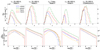 |
Fig. E.1. Differential rate of unlensed TDES for five representative models. The first row shows the TDE redshift, and the second row shows the BH mass. These figures are calculated for LSST magnitude limits. |
Appendix F: Quads time delay distributions
In Fig. F.1, we show the time delay distributions for quad lenses calculated for LSST limiting magnitudes. The earliest image is taken as the reference image. The time delay distributions for double lenses are shown in the last row of Fig. 12. The delay between the first and second image is Δt1. The distributions show that we expect this time delay to be approximately 11 days. The delay between the first and third image is Δt2. This time delay is approximately 5 days. The delay between the first and fourth image is Δt3. This time delay is approximately 3 days. We find a very similar time delay distribution to that of the double lenses. The quads exhibit signs of a low time delay tail that is not observed for the doubles. However, such systems seem rare and are only observed at numerical uncertainty.
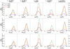 |
Fig. F.1. Histograms show the differential rate of TDEs for five representative models. Δt1 is the time delay between the first and second arriving image. Δt2 is between the first and third image. Δt3 is the first and last image. These figures are calculated for LSST magnitude limits. |
All Tables
Rate of double and quad lensed TDEs, the ratio of double to quad lenses, and the fraction of quad to total lenses.
All Figures
|
Fig. 1. Three different BHMFs we consider showing significantly different redshift evolutions. Left panel: Redshift independent BHMF from Gallo & Sesana (2019). Middle panel: BHMF derived by the TRINITY model (Zhang et al. 2023). Right panel: BHMF calculated by combining a galaxy stellar mass function (GSMF) (Davidzon et al. 2017) and a BH-to-bulge mass relation (Kormendy & Ho 2013). The z-independent BHMF has a different normalization than the other two. Up to redshift of 2, TRINITY and COSMOS2015 agree closely. |
| In the text | |
|
Fig. 2. Three different TDE luminosity functions dependent on BH mass. For low BH masses, L1 is Eddington limited. The two L2 models do not yet differ through their treatment of temperature, as temperature is not involved yet. However, they differ because of a correction factor that accounts for the spread of specific energy in the resulting debris. The T-independent model assumes this factor to be constant. |
| In the text | |
|
Fig. 3. TDE temperature dependent on BH mass using the L2 model. We assumed a solar-like star, that is, M⋆ = 1 M⊙ and R⋆ = 1 R⊙. |
| In the text | |
|
Fig. 4. Black body flux for different temperatures (upper panel) and BH masses (lower panel). For L2, T-indep. in the upper panel, |
| In the text | |
|
Fig. 5. Rate of TDEs as a function of survey limiting magnitude. The left panel shows the detection rate in the g band for the 33 models individually. We separated the color and line style information to keep the legend short. The right panel shows the detection rate in the u, r, and i bands, where each shaded region encompasses the spread in the models. We chose L2, TRINITY, 20 000 K as a fiducial model to guide the eye. The 33 models we considered for the unlensed TDE rate show a scattering factor of 𝒪(102) that can reach above 𝒪(103) for the u and i bands. The vertical black lines (left panel) and the colorful strips (right panel) show the observational magnitude limit for ZTF (g, r, i bands) and LSST (u, g, r, i bands). |
| In the text | |
|
Fig. 6. Rate of TDEs as a function of survey limiting magnitude. Only the local BHMF impacts the unlensed TDE rates observed by current and near-future surveys such as ZTF and LSST. The redshift evolution of the BHMF influences the rate from a limiting magnitude of 25 onward. We have taken a representative subset from the left panel of Fig. 5 to clearly show the influence of the BHMF. |
| In the text | |
|
Fig. 7. Rate of TDEs as a function of survey limiting magnitude for different luminosity models. The luminosity model has little impact on the unlensed TDE rate. It can introduce a dependence of the rate on the observing band for the fixed-temperature models. The temperature-dependent model can compensate for the chosen observing band by selecting the TDE temperature. Thus, it does not show a strong band dependence. We have taken a representative subset from the left panel of Fig. 5 to clearly show the influence of the luminosity model. |
| In the text | |
|
Fig. 8. Rate of TDEs as a function of survey limiting magnitude. The chosen temperature has the largest impact on the unlensed TDE rate. This parameter accounts for most of the scatter observed between the different models. This implies that it is crucial that the BB peak and the observing band are well aligned. We have taken a representative subset from the left panel of Fig. 5 to clearly show the influence of the temperature. |
| In the text | |
|
Fig. 9. Illustration of a lensed TDE with two images, A and B, around a galaxy acting as a lens. The lens has an Einstein radius, θE, that gives an estimate of the image separation, θsep. Due to the different geometric path lengths and the gravitational time delay (Shapiro 1964), we expect image B to appear later than image A with a time delay of Δt. |
| In the text | |
|
Fig. 10. Rates of lensed TDEs as a function of survey limiting magnitude. The lensed TDE rates also show a scattering factor of 𝒪(102) that can almost reach 𝒪(103). The gray strip shows the observational magnitude limit for LSST (u, g, r, i bands). We display L2, TRINITY, 20 000 K as a fiducial model in solid lines to guide the eye. |
| In the text | |
|
Fig. 11. Lensed fraction for the different TDE models. Each point represents the fraction of TDEs observed as part of a lensing system. The lines are used for the temperature-dependent L2 models. The fractions of lensed TDEs show a greatly reduced scatter than the scatter of the unlensed and lensed rates. The fractions lie within a factor of 50. We calculated these lensed fractions for the LSST magnitude limits. |
| In the text | |
|
Fig. 12. Differential rate of lensed TDEs for five representative models. The rows from top to bottom are the TDE redshifts, BH masses, lens redshifts, lens velocity dispersions, lensed image separations, and time delays of doubles. The three time delays for quads are shown in Appendix F. These figures were calculated for LSST magnitude limits. |
| In the text | |
|
Fig. B.1. Impact of a different TDE occurrence rate per galaxy on the cumulative, unlensed TDE rate. The TDE occurrence rate mainly acts as a constant offset with an overall weak influence on the TDE rate. |
| In the text | |
|
Fig. B.2. BH mass distribution for different TDE occurrence rates. These distributions are calculated for LSST magnitude limits. |
| In the text | |
|
Fig. C.1. Schematic view of a gravitational lens. The light travels along the blue path, meaning we observe the image at a different angular position θ compared to the true angular source position β indicated with the green line. |
| In the text | |
|
Fig. E.1. Differential rate of unlensed TDES for five representative models. The first row shows the TDE redshift, and the second row shows the BH mass. These figures are calculated for LSST magnitude limits. |
| In the text | |
|
Fig. F.1. Histograms show the differential rate of TDEs for five representative models. Δt1 is the time delay between the first and second arriving image. Δt2 is between the first and third image. Δt3 is the first and last image. These figures are calculated for LSST magnitude limits. |
| In the text | |
Current usage metrics show cumulative count of Article Views (full-text article views including HTML views, PDF and ePub downloads, according to the available data) and Abstracts Views on Vision4Press platform.
Data correspond to usage on the plateform after 2015. The current usage metrics is available 48-96 hours after online publication and is updated daily on week days.
Initial download of the metrics may take a while.