| Issue |
A&A
Volume 701, September 2025
|
|
|---|---|---|
| Article Number | A17 | |
| Number of page(s) | 21 | |
| Section | Planets, planetary systems, and small bodies | |
| DOI | https://doi.org/10.1051/0004-6361/202554832 | |
| Published online | 28 August 2025 | |
A reliable activity proxy in SPIRou spectra of M dwarfs using machine learning
1
Université de Toulouse, CNRS, IRAP,
14 av. Edouard Belin,
31400
Toulouse,
France
2
Center for Astrophysics | Harvard & Smithsonian,
60 Garden street,
Cambridge,
MA 02138,
USA
3
Univ. Grenoble Alpes, CNRS,
IPAG,
38000
Grenoble,
France
4
Université de Lyon, INSA-Lyon, CNRS,
LIRIS,
69621
Lyon,
France
5
Université Côte d'Azur, Observatoire de la Côte d'Azur,
CNRS,
Laboratoire Lagrange
06903,
France
6
Institut Trottier de recherche sur les exoplanètes, Département de Physique, Université de Montréal,
Montréal,
Québec,
Canada
7
Observatoire du Mont-Mégantic,
Québec,
Canada
8
Aix Marseille Univ, CNRS, CNES, LAM,
Marseille,
France
9
Laboratoire Univers et Particules de Montpellier, Université de Montpellier,
CNRS,
34095
Montpellier,
France
10
Leiden Observatory, Leiden University,
Niels Bohrweg 2,
2333 CA
Leiden,
The Netherlands
★ Corresponding author: This email address is being protected from spambots. You need JavaScript enabled to view it.
Received:
28
March
2025
Accepted:
16
June
2025
Abstract
Context. Recent instruments have extended radial velocity observations from the optical domain to the near-infrared range (NIR). In particular, this has allowed M dwarfs to be studied more extensively, which is notable because they are known to host rocky planets more frequently. However, these stars also have, on average, stronger magnetic activity compared to solar-type stars, and investigating this magnetic activity is key to uncovering any planets around such stars.
Aims. This paper aims to extensively test a new reliable magnetic activity indicator named W1 and confirm it as a proxy for the small-scale magnetic field for M dwarf stars.
Methods. The magnetic activity indicator W1 is derived from a principal component analysis (PCA) applied on the per-line differential line width (dLW). However, the PCA is highly sensitive to contamination from telluric residuals in the spectra. Therefore, we employed a filtering technique based on such machine learning tools as the unsupervised dimensional reduction (DR) algorithm and support vector machine (SVM) to remove faulty lines. We assessed the performance of this filtering method using a simulation of observations of the per-line dLW variations before applying it to NIR high-resolution spectroscopic observations from SPIRou (at the Canada-France-Hawaii Telescope) of five targets with various stellar magnetic activity levels, spectral types, and rotation periods contained in the SPIRou Legacy Survey, namely AU Mic, EV Lac, GJ1286, GJ1289, and G1 410.
Results. The filtered W1 signal is modulated with a period consistent with the rotation period retrieved from activity indicators, corresponding to the magnetic activity for all the stars studied. It also correlates with the small-scale magnetic field of all five stars, with a direct Pearson correlation coefficient greater than 0.80. Additionally, we identified 201 stellar lines that are particularly sensitive to magnetic activity that could be valuable for the study of magnetic fields.
Key words: techniques: radial velocities / techniques: spectroscopic / stars: magnetic field
© The Authors 2025
 Open Access article, published by EDP Sciences, under the terms of the Creative Commons Attribution License (https://creativecommons.org/licenses/by/4.0), which permits unrestricted use, distribution, and reproduction in any medium, provided the original work is properly cited.
This article is published in open access under the Subscribe to Open model. This email address is being protected from spambots. You need JavaScript enabled to view it. to support open access publication.
1 Introduction
Since the discovery of the first exoplanet orbiting a Sun-like star using the radial velocity (RV) method – which measures the barycentric reflex motion of stars projected along the line of sight through the Doppler shift of their spectra – nearly 30 years ago (Mayor & Queloz 1995), detection techniques and observational instruments have seen significant advancements. Modern optical spectrometers now achieve remarkable precision, measuring Doppler shifts down to approximately 0.1 ms−1 (Fischer et al. 2016; Pepe et al. 2021). Despite these improvements, the quest to detect an Earth analog remains an outstanding challenge. For instance, the reflex motion induced by the Earth on the Sun is about 9 cm s−1, a signal often obscured by stellar activity, which can produce several m s−1 of RV jitter on various timescales (Meunier et al. 2010; Lagrange et al. 2011; Haywood et al. 2014; Meunier & Lagrange 2019).
M dwarfs are promising targets for exoplanet detection, particularly for characterizing habitable Earth-like planets. Representing 75% of the stars within 10 pc of the Sun (Reylé et al. 2021), these low-mass stars are excellent candidates for detecting small rocky planets (Bonfils et al. 2013; Dressing & Charbonneau 2015; Gaidos et al. 2016; Anglada-Escudé et al. 2016; Hsu et al. 2020; Sabotta et al. 2021; Faria et al. 2022; Suárez Mascareño et al. 2023; Basant et al. 2025). Their lower mass amplifies the gravitational influence of the orbiting planets, making the RV signals easier to detect, and their lower luminosity allows for planets to reside within the habitable zone at shorter orbital distances.
However, M dwarfs exhibit stronger magnetic activity than Sun-like stars, which complicates RV measurements. Surface brightness inhomogeneities such as spots and faculae (Huélamo et al. 2008; Boisse et al. 2011; Reiners et al. 2013; Carmona et al. 2023; Larue et al., in prep.) often contribute to RV variability, but their effect is generally weaker in the near-infrared (NIR) compared to the optical. On the other hand, Zeeman broadening – proportional to wavelength squared (Reiners 2012; Reiners et al. 2013; Hébrard et al. 2014; Kochukhov 2021)–becomes stronger in the NIR, adding another layer of complexity. Additionally, telluric absorption is more pronounced in the NIR, further challenging precise RV measurements. These factors highlight the importance of carefully characterizing stellar magnetism to improve exoplanet detection, particularly for M dwarfs.
To address these challenges, the Spectro-Polarimètre InfraRouge1 (SPIRou) was designed to detect planets around M dwarfs while simultaneously characterizing their magnetic fields to enhance planet detection capabilities (Donati et al. 2020). Under the SPIRou Legacy Survey2 – Planet Search (SLSPS; Moutou et al. 2023) program, complemented by the SPICE3 follow-up program, spectroscopic observations of ∼ 50 nearby M dwarfs with varying magnetic activity levels were conducted over 5 years. These data allow for a detailed line-by-line analysis of stellar spectra (Artigau et al. 2022), providing crucial insights into both planetary signals and stellar activity.
This paper highlights the viability of the magnetic activity proxy W1, first introduced in Donati et al. (2023), derived from a principal component analysis (PCA) on width variations of individual stellar lines, as they might be broadened by the Zeeman effect or appear deeper or larger with surface temperature variation, as described in Section 3. W1 is sensitive to telluric residual contamination, a challenge we explore through a toy model in Section 4. The methodology for mitigating this contamination is outlined in Section 5, and the results are presented in Section 6. The five SLS/SPICE targets studied are introduced in Section 2. We conclude with a discussion of our findings in Section 7.
2 Observations
2.1 Observational facilities
All observations were obtained within the framework of the SLS (Moutou et al. 2023) and the SPICE programs using SPIRou, a high-resolution near-infrared spectropolarimeter, installed in 2018 at the Cassegrain focus of the Canada-France-Hawaii Telescope (CFHT). It operates in a spectral range of 0.98 μm to 2.35 μm, with a resolution power of 70 000. A detailed overview of the instrumental design and initial performances can be found in Donati et al. (2020).
All SPIRou spectra were reduced using APERO4 (A PipelinE to Reduce Observations), detailed in Cook et al. (2022). APERO produces science frames and generates 2D and 1D spectra for three fibers (two science channels and one reference channel). Employing the TAPAS model spectrum of the Earth's atmosphere (Bertaux et al. 2014) and a library of hot star spectra obtained under various air-mass and humidity conditions with SPIRou, APERO performs a three-step telluric correction approach on the science spectra. The work for this paper was performed on reduced data using version 0.7.290 of APERO and the Line-By-Line (LBL) version 0.64.013.
2.2 Small-scale magnetic field
The small-scale magnetic field (noted 〈B〉) is known to be an efficient proxy for stellar activity jitter in the case of the Sun (Haywood et al. 2016) and Sun-like stars (Haywood et al. 2022). Cristofari et al. (2023) developed a process to systematically constrain the atmospheric parameters (Teff, log g, [M/H],[α/Fe]), and the unsigned magnetic flux by comparing models of spectra computed with ZeeTurbo to high-resolution spectra. ZeeTurbo calculates spectra from the MARCS model of stellar atmospheres (Gustafsson et al. 2008). The code combines Turbospectrum (Alvarez & Plez 1998; Plez 2012) and Zeeman (Landstreet 1988; Wade et al. 2001; Folsom et al. 2016) to account for the Zeeman effect and polarized radiative transfer in selected atomic lines, allowing it to estimate the small-scale magnetic field from unpolarized Zeeman broadening. Further details on the method can be found in Cristofari et al. (2023). Figure 1 presents the 〈B〉 time series and periodograms of the targets AU Mic, EV Lac, GJ 1289 and Gl 410 while small-scale magnetic field of GJ1286 in presented in a separated figure (Fig. 2).
Previous study by Donati et al. (2023) discussed that the small-scale magnetic field is potentially a relevant proxy for M dwarfs, based on the case of AU Mic, where the time derivative of the small-scale magnetic field (reconstructed using a Gaussian Process) correlates with the RV signal with a coefficient of up to 0.78. In the same study, Donati et al. (2023) noticed that the first component of the PCA analysis of per-line differential Line Width (dLW)−W1− is strongly correlated to the small-scale magnetic field with a direct Pearson-R correlation score of 0.96 for AU Mic. In the following sections, we systematically compare this metric to the activity indicator W1.
However, deriving the small-scale magnetic field is computationally expensive and requires a relatively high signal-to-noise ratio (S/N) spectra (Cristofari et al. 2023). For this study, we only have access to time-series measurements for a limited subset of targets from the SLS/SPICE programs. If we can identify a reliable proxy for 〈B〉 from the byproducts of RV data processing, it could serve as a direct activity indicator, facilitating the filtering of RV stellar jitter in active stars.
2.3 Targets
Among all the targets of the SLS-PS (Moutou et al. 2023) and SPICE programs, we focused on a set of five stars with various spectral types, rotation periods and observation conditions. Those stars are namely AU Mic, EV Lac, GJ1286, GJ1289 and Gl 410. In this article, we chose a small representative stellar sample to develop the new activity proxy and study its significance with respect to other ones such as the small-scale magnetic field measurements, presented in Figures 1 and 2. Table 1 provides a comprehensive overview of the stellar parameters for the examined targets. All observations were conducted at the CFHT between April 2019 and October 2023.
2.3.1 AU Mic
AU Mic (or Gl 803) is a young (23 Myr; Mamajek & Bell 2014) and nearby (d = 9.714 ± 0.002 pc; Gaia Collaboration 2018) M1 star. As expected for such young stars, its magnetic activity is intense. Its average surface magnetic field is 2.71 ± 0.13 kG (Cristofari et al. 2023). Its surface brightness inhomogeneities and frequent flares are causing huge photometric and RV variations (Plavchan et al. 2020). SPIRou observations of AU Mic have previously been used in spectropolarimetric analyzes to characterize the evolving magnetic field topology of AU Mic (Klein et al. 2021; Donati et al. 2023). Moreover, AU Mic is known to host at least two transiting planets (Plavchan et al. 2020; Martioli et al. 2021; Szabó et al. 2021; Gilbert et al. 2022; Szabó et al. 2022), with two other candidates reported by Wittrock et al. (2023) and Donati et al. (2023). Its intense and deeply studied magnetic activity and the presence of known planets makes AU Mic the ideal study case to test our activity indicator. Furthermore, the activity indicator presented in this study was firstly explored in Donati et al. (2023) on AU Mic showing a clear correlation with small-scale magnetic variation of this star.
On its small-scale magnetic field (Fig. 1, panel a), the periodogram clearly shows modulation with the star's rotation period (4.859 ± 0.004 d; Donati et al. 2023), consistent with photometric observations (4.863 ± 0.010 d; Plavchan et al. 2020; 4.85 ± 0.03 d; Gilbert et al. 2022). The amplitude of this modulation varies over time between 0.1 and 0.25 kG. A detailed analysis of AU Mic's 〈B〉 time series has already been conducted in Donati et al. (2023), to which we refer the reader for further insight.
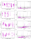 |
Fig. 1 Small-scale magnetic field measurements from ZeeTurbo (Cristofari et al. 2023) using SPIRou spectra for AU Mic, EV Lac, GJ1289, and Gl 410, along with their periodograms. The black horizontal lines (solid, dashed, dotted) indicate false alarm probabilities of 10%, 1%, and 0.1%. The vertical blue dashed line marks the literature rotation period. The gray curve represents the window function, illustrating time sampling effects. |
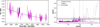 |
Fig. 2 Small-scale magnetic field measurements of GJ1286 along with its periodogram. In this case the periodogram has been obtained by first removing a quadratic trend. The periodogram of the original data is still visible (purple dotted lines). The dashed vertical line indicates the second harmonic of the rotation period while the other vertical and horizontal lines were already presented in Fig. 1. |
Reported stellar properties from the literature for our target sample.
2.3.2 EV Lac
EV Lac (or Gl 873) is a nearby M3.5V red dwarf star (d=5.05 pc; Gaia Collaboration 2018). It is one of the most widely studied low-mass stars due to its strong small-scale magnetic field (〈B〉=4.59 ± 0.29 kG; Cristofari et al. 2023) and frequent stellar flares (Muheki et al. 2020; Paudel et al. 2021; Chen et al. 2022 and references therein). Zeeman Doppler Imaging (ZDI; Donati & Brown 1997) studies by Morin et al. (2008) and Bellotti et al. (2024) have shown that EV Lac's large-scale magnetic topology evolves over time and exhibits unexpected complexity. On a large scale, its longitudinal magnetic field (i.e., the line-of-sight projection of the magnetic field vector averaged over the visible stellar hemisphere, equal to several tens of G, Moutou et al. 2018) shows broad variation that can reach an amplitude of 149 ± 17 G (Fouqué et al. 2023). These characteristics make EV Lac an interesting target for testing our new proxy for stellar magnetic activity.
The rotation period measured by Morin et al. (2008) is 4.3615 ± 0.0001 d, while photometric observations by Díez Alonso et al. 2019 determined Prot = 4.379 ± 0.010 d. The star's rotation plays a key role in modulating its small-scale magnetic field as well. An analysis of the time series of 〈B〉 (Fig. 1, panel b) reveals a modulation period of 4.362 ± 0.001 d with a semi-amplitude of  kG (Cristofari et al., in prep.), which remains relatively stable over the observed time span. This period is consistent with the rotation periods reported in the literature (Morin et al. 2008; Díez Alonso et al. 2019; Bellotti et al. 2024).
2.3.3 GJ1289
GJ1289 is a fully convective M4.5Ve star located at 8.3535 ± 0.0081 pc from the earth (Gaia Collaboration 2018). Its average small-scale magnetic field is relatively high (〈B〉= 1.01 ± 0.08 kG; Cristofari et al. 2023). From measurements of the longitudinal magnetic field, Fouqué et al. (2023) and Donati et al. (2023) report that its semi-amplitude can reach up to 70 G, comparable to the most active stars in the SLS program (e.g., 45 ± 6 G for AD Leo's Bl modulations, Carmona et al. 2023, and 149 ± 17 G for EV Lac, Fouqué et al. 2023). The modulation period of the longitudinal magnetic field was fitted by both Fouqué et al. (2023) and Donati et al. (2023) and they derived a rotational period of  d and 73.66 ± 0.92 d respectively. Those values are compatible with each other and within the 2 σ confidence interval measured using photometry (86.3 ± 7.0 d; Díez Alonso et al. 2019). Moutou et al. (2024) recently found a sub-Neptune in a circular orbit around GJ1289 with 111.74 d of period.
From the periodogram of the small-scale magnetic field, we measured a modulation period of  d (Fig. 1 panel c), compatible with the rotation period given in the literature (Fouqué et al. 2023; Donati et al. 2023), with a semi-amplitude of
  kG. On top of that, we clearly see a long-term modulation of
  d. This signal is stronger than the rotational modulation, according to the periodogram, varying between 0.8 kG and 1.6 kG with an average semi-amplitude of
  kG.
kG.
2.3.4 GJ1286
GJ1286 is located at 7.1782 ± 0.0054 pc from the Earth (Gaia Collaboration 2018). It is the least massive star of our sample (its spectral type being M5.5). It is a slower rotator than GJ1289 but it shows similar properties. The exact value of its rotational period is, however, still not well constrained. Fouqué et al. (2023) and Donati et al. (2023) found respectively  d and 178 ± 15 d from the longitudinal magnetic field derived from SPIRou spectropolarimetric data. Lehmann et al. (2024) measured a rotation period of
  d, performing a PCA on the Least Square Deconvolution (LSD) Stokes V profiles. Photometry measurements provide a rotational period of 88.92 d (Newton et al. 2018) which is consistent with the second harmonic of the signal that has been measured in spectropolarimetry (Fouqué et al. 2023; Donati et al. (2023); Lehmann et al. 2024).
The small-scale magnetic field of GJ1286 (Fig. 2) decreases by ∼ 1 kG over the observed time span, going from 1.93 ± 0.31 kG in the first bin to 0.83 ± 0.19 kG on the last one. Once detrended using a quadratic function, the signal shows variations at a recurrence period of  d that is compatible with the rotation period of the star measured in photometry (Newton et al. 2018) and half the period measured in spectropolarimetry (Fouqué et al. 2023; Donati et al. 2023; Lehmann et al. 2024). The semi-amplitude of this rotational variation seems to decrease along with the global small-scale magnetic field, from a semiamplitude of 0.28 kG in the first half of the measurements to 0.11 kG at the latest.
The relatively strong magnetic fields of GJ1289 and GJ1286 are reminiscent of faster rotating M dwarfs in the saturated dynamo regime such as AU Mic and EV Lac, which is surprising for such slow rotators given their Rossby number R0 larger than unity, as discussed in Lehmann et al. (2024). Therefore, these two targets are particularly interesting stars for our study, offering a diverse range of rotational periods to test our methods.
2.3.5 GI 410
Gl 410 (or DS Leo) is a 0.55 ± 0.02 M☉ M1 star (Cristofari et al. 2022) located at 11.938 ± 0.0029 pc from the Sun (Gaia Collaboration 2018). From SPIRou spectra, Fouqué et al. (2023) and Donati et al. (2023) measured similar rotation periods of  d and 13.91 ± 0.09 d, respectively. Previous study by Hébrard et al. (2016), reported a noticeable differential rotation with Prot = 13.37 ± 0.86 d at the pole and 14.96 ± 1.25 d at the equator. In photometry, Díez Alonso et al. (2019) recorded a period of 14.6 d, while Giacobbe et al. (2020) found a 15.3093 d modulation. ZDI analysis by Hébrard et al. (2016) revealed a strong toroidal large-scale magnetic field with significant variability, probably due to strong surface differential rotation. Running the Paul23b code on SPIRou spectra of Gl 410 yielded an average small-scale magnetic field of 0.71 ± 0.03 kG (Cristofari et al. 2023), measured from the stellar template. Additionally, Carmona et al. (2025) identified a candidate exoplanetary system around Gl 410 using SPIRou spectra.
Its small-scale magnetic field (Fig. 1 panel d) clearly shows a rotational modulation in the periodogram with a measured period of 13.982 ± 0.074 d (Cristofari et al., in prep.). We also observe a global variation of 〈B〉 with a minimum reached between 2021B and 2022A (Fig. 1 panel d). This global evolution leaves an imprint in the peridogram as a ∼ 1000 d modulation signal. Such long-term modulation could possibly originate from an evolving magnetic topology through magnetic cycles as monitored by Lehmann et al. (2024) for GJ1286, GJ1289 and several other targets within the SLS program.
3 Activity indicators of line-by-line RV measurements
From SPIRou spectra reduced with APERO, we usually extract the RVs through the LBL5 (Artigau et al. 2022) method. This method is based on the framework developed by Bouchy et al. (2001) and initially proposed by Dumusque (2018), was subsequently explored in the context of optical RV observations with HARPS by Cretignier et al. (2020) and adapted to NIR spectrometers, including SPIRou, by Artigau et al. (2022). Within the LBL framework, RVs are derived by comparing for every single line6 the residuals of the observed spectrum A(i) with the template A0(i) and the template's derivative. By extending this framework to further components of the Taylor series, one can link the dLW to the second derivative. This extended the Bouchy equation (Bouchy et al. 2001) to give Eq. (1) (Artigau et al. 2022):
 (1)
with λ(i) as the wavelength of pixel i, δ V(i) as the RV shift between A(i) and A0(i), and c as the speed of light.
(1)
with λ(i) as the wavelength of pixel i, δ V(i) as the RV shift between A(i) and A0(i), and c as the speed of light.
Beyond providing a mean RV value for the stellar spectrum, the LBL method provides per-line RV time series. The perline time series allows for the application of statistical methods such as a weighted PCA (wPCA; Delchambre 2015) enabling refinement of the global RV time series as demonstrated by Ould-Elhkim et al. (2023) in the framework of the Wapiti method. Similarly to RVs, the LBL framework allows for the application of statistical methods on dLW as well. As the line width of lines can be enlarged due to the Zeeman effect7, dLW is known to be a good activity indicator (Zechmeister et al. 2018; Artigau et al. 2022; Schöfer et al. 2022). The presence of spots may also induce variations in the measured line width (Huélamo et al. 2008; Boisse et al. 2011; Reiners et al. 2013; Hébrard et al. 2014; Carmona et al. 2023; Larue et al., in prep.). Applying statistical methods such as wPCA on this LBL byproduct could refine the capabilities of this activity indicator. This has been introduced in Donati et al. (2023) where the authors found that the first component of the dLW wPCA, hereafter W1, is a promising activity proxy for the small-scale magnetic field, in the case of AU Mic, by reporting a direct Pearson correlation coefficient of 0.96 between W1 and 〈B〉 (Donati et al. 2023). As previously mentioned in Sec 2.2, 〈B〉 is already known to be a good indicator for the RV stellar jitter of the Sun (Haywood et al. 2016) and Sun-like stars (Haywood et al. 2022) (direct correlation) and the M dwarf AU Mic (Donati et al. 2023) (RVs correlate with the first time derivative of 〈B〉). Thus, its proxy W1 is also a good candidate as an activity indicator and could be employed to filter magnetic activity in RV data and thus help uncover potentially embedded planets. The main goal of this study is to confirm W1 as a proxy for the small-scale magnetic field on M dwarfs.
4 Simulating and characterizing the sensitivity of the activity indicator to telluric contamination with a toy model
SPIRou operates in the infrared, a domain heavily contaminated by telluric lines. APERO corrects the telluric lines very efficiently (Cook et al. 2022) using model spectrum of the Earth atmosphere (Bertaux et al. 2014) and a library of hot star spectra obtained under various airmass and humidity conditions. Previous studies have estimated that the imprint of a telluric line is reduced to a few percent of the continuum level (Artigau et al. 2014; Sameshima et al. 2018; Ulmer-Moll et al. 2019; Artigau et al., in prep.; Ould Elhkim et al., in prep.) for various pipelines and spectrometers. Even reduced, these residuals can affect the final RV measurements (Wang et al. 2022; Latouf et al. 2022). In the case of SPIRou, Ould-Elhkim et al. (in prep.) have recently showed that the presence of tellurics, even when corrected at a residual level of 3% of the continuum level, can lead to yearly signals and its harmonics in the RV data, and suggests that this also occurs for dLW. Therefore, it is important to determine whether other variability sources than the activity modulation, such as telluric contamination, may hamper the analysis of W1. The residual contamination can vary greatly from one stellar line to another. Depending on the relative positions of stellar lines and contaminating terrestrial lines, the latter's effect on stellar lines will have a certain phase and amplitude, and can also vary over time depending on atmospheric conditions. Thus, the imprint of this contamination can appear to be random from line to line. Because of this variability, the effect of this telluric contamination might not be immediately dominant in the overall time series of dLW when averaged (except for a global off-set). However, wPCA is more sensitive to that kind of variation as demonstrated in Ould-Elhkim et al. (in prep.). It has been designed especially for the purpose of unveiling the main source of variations over multiple time series. Thus, the first wPCA component of dLW, W1, will be even more likely contaminated by the tellurics than the averaged dLW time series.
To illustrate this phenomenon, we built a simple toy model. The model is derived from real observations of EV Lac with SPIRou whose behavior we aim to reproduce. For every single line of the template spectra, we recorded its depth (a0), width (σ0), and wavelength (λ0) by approximating the line shape as a Gaussian. This Gaussian line was then considered as the template A0(i).
 (2)
Then, we simulated observations, A(i, t), of this line for every epoch. There are three main components of the line. The first is the line itself, which is a Gaussian line that has the same depth (a0) and wavelength (λ0) as recorded for the template but with a slightly different width that has been incremented by a differential width σ=σ0+Δ σ. This differential width, Δ σ, is scaled using a normalized Gaussian process of the small-scale magnetic field measurements of EV Lac (see Fig. 1 panel b) multiplied by the measured dLW amplitude of this particular line for a periodic signal of Prot = 4.3615 d in real EV Lac LBL data.
(2)
Then, we simulated observations, A(i, t), of this line for every epoch. There are three main components of the line. The first is the line itself, which is a Gaussian line that has the same depth (a0) and wavelength (λ0) as recorded for the template but with a slightly different width that has been incremented by a differential width σ=σ0+Δ σ. This differential width, Δ σ, is scaled using a normalized Gaussian process of the small-scale magnetic field measurements of EV Lac (see Fig. 1 panel b) multiplied by the measured dLW amplitude of this particular line for a periodic signal of Prot = 4.3615 d in real EV Lac LBL data.
To account for residual telluric contamination in our model, we use a TAPAS atmospheric transmission spectrum (Bertaux et al. 2014), which is first convolved with the instrumental profile to simulate the resolution of real observations. Each telluric line is characterized by its central wavelength (λt), depth (at), width (σt), and molecular species. We model each line as a Gaussian profile and record its properties accordingly. When a telluric line overlaps with the wavelength range of a stellar line, it is injected into the stellar spectrum as a Gaussian feature. To simulate observational conditions, the telluric line is first Doppler-shifted according to the barycentric Earth radial velocity (BERV), ensuring a realistic representation of the Earth's motion relative to the star. Then, to account for imperfect telluric correction, its depth is scaled to 3% of its original value with a scatter of ± 1%, modeled as a normal distribution. To introduce additional variability, we further adjust the telluric depths to reflect changes in atmospheric conditions. Specifically, before applying the residual correction factor, we scale the depth of each telluric line using an exponent corresponding to the recorded humidity for water lines and the airmass for other molecular species, capturing the influence of varying atmospheric parameters on telluric absorption.
We finally add some photon noise to the observed line at the amplitude level that correspond to the S/N of the order of that line in the detector. Due to the correction and interpolations in the processing steps of APERO or possible modal noise in the fibers (Micheau et al. 2018; Blind 2022), the spectral noise observed in APERO corrected SPIRou spectra is not exactly the white photon noise anymore. There is a lack of high frequencies in the power spectral density (PSD) of that noise. In order to inject a realistic noise that corresponds to the real spectra on which we later apply our LBL routine, we modeled the PSD of the observed spectral noise with a custom function and then injected the noise corresponding to that PSD function. This process is detailed in Appendix A.
The final form of the simulated line for each time sample is then
 (3)
(3)
Finally, we applied the LBL routine – Equation (1) – and we recorded the fit parameter dLW (and its error) for every iteration of time and for every single line. This represents a total of 14 758 lines computed on 164 epochs.
We then performed a weighted PCA to get its first principal component W1. These results can be seen in red in Fig. 3. While the contamination might be faint for the weighted average, with the effect of the tellurics being canceled while averaging on the first component of the wPCA. However, the simulated atmospheric contamination dominates in Fig. 3, and the direct Pearson-R correlation score of W1 with the injected width variation signal is only about R = 0.52. The use of wPCA, rather than relying solely on the averaged time series, was intended to isolate the magnetic activity signal from other sources of variation more effectively. While averaging can suppress telluric contamination, wPCA provides a systematic framework to identify and separate distinct sources of variability. However, for this approach to be successful, it is essential to filter out the atmospheric contamination if it dominates the primary components, as demonstrated with this simulation.
 |
Fig. 3 W1 signal of the simulated dataset before (red) and after (blue) our filtering technique. The left panel is the time series, the middle panel is its LS-periodogram, and the right panel is W1 as a function of the BERV. The gray curve represents the window function, illustrating time sampling effects. |
5 Filtering method
We constructed a robust data-driven method aimed at filtering out telluric contamination from our activity indicator, W1. In this Section, we test this method on the simulated data obtained following the process described in Section 4 to ensure its proper functioning. We then discuss its application to observed spectra in Section 6.
5.1 Frequency space
As already mentioned in Section 4, the imprint of telluric contamination is not regular from one line to another, due to differences in phase of this imprint and its time variability. However, the contaminating lines are shifted back and forth (in the stellar lines barycentric reference frame) over a 1 yr period. We retrieve this periodicity and their harmonics in the generalized Lomb-Scargle (GLS) periodograms (Zechmeister & Kürster 2009) of the dLW signal of the contaminated lines. If we are looking for specific patterns to detect and eliminate contaminated lines, switching to the frequency space is more convenient. Thus, we compute the LS-periodograms of the dLW signal for each individual line. In this context, we expect that contaminated lines will induce peaks in the fundamental and harmonics of a one-year signal in their dLW periodograms, regardless of the phase or the specific pattern of that signal. Similarly, the embedded activity signal is expected to exhibit peaks at the rotation period (or at its second harmonic, as in the small-scale magnetic field of GJ1286), with varying strength depending on the line's sensitivity to the magnetic activity.
5.2 Unsupervised dimensional reduction
To disentangle the lines, we apply an unsupervised dimensional reduction algorithm to the periodograms of per-line dLW time series. Dimensional reduction (DR) tools enable the visualization of N-dimensional data in a lower dimension projection. These algorithms are designed in such a way that measurements with closely aligned properties in the original N-dimensional space, per-line dLW periodograms in our case, will remain near each other on the final map (Wattenberg et al. 2016). Some details about the construction of this map in the case of the specific algorithm used here are provided in Appendix B. Consequently, this allows for cluster analysis and the spatial disentanglement of the data based on their distribution in the final map. For a deeper understanding of how dimension reduction tools work, we refer the reader to Wang et al. (2021) and the references therein and to Appendix B for a comprehensive summary. In the context of this study, the N-dimensional measurements correspond to the recorded powers of the periodogram on the same frequency grid. In this specific framework, lines with similar dLW variations according to their periodogram would be in the same area in the 2D space. Thus, we expect contaminated lines to exhibit similar periodogram with peaks at one year or the associated harmonics, thereby staying within the same region on the final map. Similarly, lines primarily influenced by the stellar activity signal are expected to generate power at the rotation period (or its second harmonic), positioning them in another distinct area. Consequently, we can segment the resulting map to effectively distinguish telluric-contaminated lines from those showing activity.
We chose a frequency grid of 1000 bins spaced on a logscale between 1.25 and 1000 days in period. This distribution aims to uniformly represent low and high periodicities. The powers are recorded for every single line studied. This data table is then transformed into a 2D map using the algorithm PaCMAP8 (Wang et al. 2021). Among all the algorithms tested (t-SNE, Van der Maaten & Hinton 2008; UMAP, McInnes et al. 2018; TriMap, Amid & Warmuth 2019), we chose PaCMAP for its significantly faster run-time and balanced preservation of both global and local structure allowing for a better spatial dissociation between lines dominated by high or low frequency signals in the case of our study (refer to Wang et al. 2021 and Huang et al. 2022 for a complete benchmark).
In the specific case of the simulated data, the resulting projection map of per-line dLW periodogram is presented in Fig. 4. For a brief explanation on the construction of those figures, we refer the reader to Appendix B and to Wang et al. (2021) for the complete one. In this figure, the lines are color-coded based on the strongest peak in their dLW periodogram. Lines dominated by the injected line width modulation period Prot are in blue in Fig. 4 while lines dominated by modulation at a one year period will be displayed in red and its second harmonic in orange, the third one in a chartreuse color, etc. The size of the points is scaled with the log False Alarm Probability (FAP) of this dominant signal. For the map Fig. 4, we notice several structures in the obtained projection. On the left side of the figure there is a concentration of all the lines dominated by the injected width modulation, emulating the activity, as indicated by its predominant blue color. From the main cluster there is even a separate one emerging, containing the lines with the strongest activity signal as indicated by the size of their points. Going from the left side of the figure to the right, the lines are increasingly polluted by the telluric residuals, as can be seen by there being more and more red, orange, chartreuse... points, with these colors completely dominating the rightmost side of the map. We notice a third emerging cluster on the top of the figure which contain lines strongly affected by both the activity and the telluric residual absorption. We expect that our process applied to observation data will result in a more mingled disposition between those features compared to results on the model.
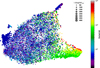 |
Fig. 4 PaCMAP map of reduced dLW periodograms of the simulated data. The color map indicates the period in days of the strongest peak in the periodogram of that line. |
 |
Fig. 5 Support vector machine separation of the output PaCMAP map. The SVM has been fed using two clouds of points corresponding to lines identified as telluric contaminated (yellow points) or sensitive to the activity (purple point). The SVM has identified their two relative areas. |
5.3 Spatially disentangling lines using support vector machine
In the following, we attribute a priori the “activity” class to the lines that are dominated by a modulation at the stellar rotation period (with an error window of ± 5% to address possible differential rotation and error bars in the rotation period given in the literature). In practice, we also select lines with modulations at Prot/2 to address cases such as GJ1286 where the activity signal manifests variations at the second harmonic of the rotation period as well. The preselected lines are represented in purple in Fig. 5. On the other hand, we attribute a priori the class “telluric” to the lines that are dominated by a one-year signal or harmonics (1 yr → red; 1/2 yr → orange; 1/3 yr → chartreuse), still with a ± 5% window. These lines are depicted in yellow in Fig. 5. The color codes only the period of the highest peak in the periodogram, but several relatively strong signals could coexist for some lines. This explains why the two different predetermined groups overlap with each other. In our example, initially, 1723 lines are labeled in the activity group, while 243 are in the telluric group. The other lines that do not fall into either of these two classes are temporarily not categorized (they are the gray points in Fig. 5). The relative number of lines in each predefined category (and thus the following results) is expected to vary from one star to another according to various factors such as the S/N, the residual contamination level, the relative position between stellar lines and telluric lines (i.e., the systemic radial velocity of stars), the intensity of the magnetic activity and its periodicity, etc.
The previously categorized lines can be sorted into two clouds of points, with our objective being to find the optimum separation between them. To achieve this, we employed support vector machines (SVMs), a machine learning tool specifically designed for two-group separation problems (Boser et al. 1992). SVMs have since been extended to handle multi-groups, non-linear, and overlapping distributions (Cortes & Vapnik 1995). In this study, we use the non-linear Radial Basis Function (RBF) kernel, a popular kernel used in machine learning, especially in SVM classification (Chang et al. 2010). For better boundary delineation, we assign a different weight to each line (Banjoko et al. 2019), depending on the relative power of their strongest periodic signal (represented by the size of the points Fig. 4 & 5). Thus, lines with more powerful and significant signals will count for more in the classification boundary decision.
By running the SVM in this configuration on the simulated data, we automatically identify the best separation between the two clouds of points, dividing the map into two distinct areas, as shown in Fig. 5. The purple area of Fig. 5 is the area dominated by lines whose width varies with magnetic activity (the purple points in Fig. 5). Similarly, the yellow area in Fig. 5 is the area dominated by the lines a priori contaminated by tellurics (the yellow points). Subsequently, we consider every line in the activity-dominated area (depicted as the purple area in Fig. 5) as activity-sensitive. This includes previously unlabeled lines (the gray points) and even lines that were previously labeled as telluric contaminated (19 of them). Similarly, every line in the tellurics area (depicted as yellow in Fig. 5) is considered to be telluric-polluted, including those initially assigned as activity-dominated (8 of them). Lines identified as telluric-polluted are then discarded from this study. In this example it means that we discard the 657 lines that are in the telluric-contaminated area, out of the 14758 lines initially considered. Retrospectively, the relative size of the telluric-polluted area could be an indicator of the efficiency of the telluric correction of APERO for the star studied. However, many factors could have a similar impact, such as the amplitude and periodicity of the magnetic activity and the S/N, among others, as depicted previously.
Summary of the filtering process results.
5.4 Recomputing wPCA
Finally, we recompute the wPCA of the lines remaining in the activity area. As depicted in blue in Fig. 3, the W1 signals have been effectively cleared from tellurics. Tellurics no longer contribute significantly to the main source of variability, and the primary source of variability, represented by W1, is now solely the injected stellar activity. This is evident from the prominent peak at the stellar rotation period. No correlation is observed with the BERV signal, and the correlation with the injected activity signal is now about R = 0.88 (versus R = 0.52 previously). We have therefore successfully filtered out the telluric residual contamination from the W1 signal. Since the wPCA is recomputed on the filtered dataset, the variance captured by each principal component is necessarily different from that of the original analysis. In particular, the first principal component reflects the dominant source of variance within the new subset, which may lead to changes in the relative dispersion of the projected data. This explains why the first principal component appears more (or less) scattered in the figures after filtering, as it is now computed from a different dataset.
6 Results
On observation data, a few preprocessing steps are needed before applying our filtering method. They essentially consist in grouping per night all observations into night binned datasets and then remove all lines where half of the dLW measurements are missing either because of deep telluric lines or a divergence in the computation of LBL. Thus, not all the stellar lines in the spectra are considered. These steps are similar to the preprocessing steps of Wapiti (Ould-Elhkim et al. 2023; Ould Elhkim et al. in prep). The total number of nights is indicated in Table 1 while the total number of lines considered is reported in Table 2.
6.1 AU Mic
The S/N of AU Mic's spectra are very high (384 on average), making measurements on this star less sensitive to spurious signals. Furthermore, AU Mic exhibits some of the largest magnetic field variations among the SLS/SPICE targets. As a result, even without any filtering, the first principal component of the dLW measurements already captures the activity signal. This W1 signal is strongly correlated with the small-scale magnetic field, with a Pearson correlation coefficient of R = 0.93. Both analyses reveal a strong peak at the stellar rotation period, reinforcing previous findings (Donati et al. 2023). The case of AU Mic's W1 signal has already been extensively covered in Donati et al. (2023), particularly in section 7. For a comprehensive review, we refer the reader to that work. This signal and its periodogram are shown in Fig. 6.
With this example we ensure that our filtering method does not alter the existing activity signal. The correlation of the “filtered” W1 with 〈B〉 is not altered. The PaCMAP map obtained through that process is presented in Fig. 7. At the bottom of this figure, there is an emerging cluster of lines that are dominated by a modulation period equal to the rotation period, as indicated by its color. Furthermore, this periodic signal has a relatively strong power for those lines as suggested by the sizes of the points indicating that, for those lines, dLW varies strongly with the rotation period and seems to be very sensitive to the magnetic activity without being affected by other phenomena. It would be interesting to isolate and study more in detail those particular lines. This is discussed further in Section 6.6. There are significantly fewer lines in LBL files (almost by half compared to the others), and thus significantly fewer lines considered for AU Mic due to its important Doppler broadening (v sin i =8.5 ± 1 km s−1; Donati et al. 2023) that blends lines within each other.
6.2 EV Lac
For EV Lac, at first, before filtering it, a modulation signal at Prot is present with a false alarm probability bellow 0.1% (log FAP = −7.9). However, this W1 signal is dominated by three signals that all correspond to the harmonics of the one-year signal with periods of respectively 1/2 yr, 1/3 yr and 1 yr, sorted by their power in the periodogram (see Fig. 8 where the red lines and dots are the state before filtering). The log FAP of the 1/2 yr signal is −18.9. The correlation coefficient between 〈B〉 and W1 is R = 0.61. The behavior of the EV Lac's W1 signal (in red on the Fig. 8) is very similar to the simulated data (as expected since we set up this model to mimic EV Lac's behavior).
While applying our filtering technique, at first we flagged 721 and 977 lines respectively for the “activity” and the “telluric” groups on which we had run the SVM. The overlap between the preselected “activity” lines from real and simulated data is not significant due to both the randomness and the simplicity of the model. The activity area found by the SVM, on which we recomputed the wPCA, contains 60% of all the lines considered. The produced PaCMAP map in the process and the SVM delineation are displayed in Fig. 9. Recomputing the wPCA only on the remaining lines completely solves the telluric issue. The filtered W1 signal does not correlate at all with the BERV and strongly correlates with the small-scale magnetic field (R = 0.96). The W1 signal now only contains the rotational modulation without any other spurious signals (see the blue dots, Fig. 8). On the PaCMAP map displayed in Fig. 9, we noticed an emerging cluster of lines solely and strongly affected by the magnetic activity as in AU Mic's map, this time in the upper-left corner of the figure.
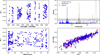 |
Fig. 6 Top left: W1 time series of AU Mic before (red) and after (blue) our filtering technique. Top right: the periodogram of this time series. Bottom left: W1 signal of AU Mic as a function of the BERV. Bottom right: W1 signal of AU Mic as a function of the small-scale magnetic field, <B>. |
 |
Fig. 7 PaCMAP map of reduced LBL dLW periodograms of the star AU Mic. The color map indicates the period in days of the strongest peak in the periodogram of that line, while the size of the point indicates its relative power. |
6.3 GJ1289
In the initial W1 times series of GJ1289, Fig. 10, the telluric residual contamination dominates with periodicities such as 1 yr or 1/3 yr (and 1/2 yr way fainter, see the initial state in red in Fig. 10). The log FAP of the 1 yr signal is −103.0. The log FAP of a modulation corresponding to the rotational period is only about −0.8 for this principal component and is far from being the dominating signal. The correlation between the initial W1 and the small-scale magnetic field signal is very low (R = 0.06). Meanwhile, W1 correlates strongly with the BERV with, especially for BERV <−20 km s−1 as visible in Fig. 10. To find a component that could be related to activity, we have to look at the third one (W3). This component correlates with the small-scale magnetic field with a coefficient of R = 0.73, but the periodogram of this component reveals several long period signals more significant than the known rotation period.
A telluric residual decontamination is obviously needed for this star. By doing so, we first identified 1237 and 1668 lines, respectively, that are dominated by activity and telluric contamination. By training the SVM on these two groups and recomputing the wPCA on the identified activity area then found, the first vector is now free from telluric contamination. In the recomputed W1, the rotational modulation is now the dominating signal, with a log FAP of −39.6 and correlates with 〈B〉 at a level of R = 0.83. The filtered W1 has the same properties as the small-scale magnetic field, which are its visible Prot variations and a ∼ 1000 day modulation. The W1 signal is recomputed from approximately 75% of the studied lines. The map obtained via PaCMAP and the separation found by the SVM can be found in Fig. 11. Once again, an activity cluster seems to emerge in the upper-right corner of the figure. We notice that on the BERV-folded space, some significant structures are left in the filtered W1 (lower-left panel of Figure 10). These structures are induced by the relatively long period of the W1 modulation which produces these artifacts when phase-folded at 1 yr. In fact, BERV-folding the 〈B〉 signal (that is considered telluric-free) produces the same structures, which reinforces our analysis.
 |
Fig. 8 W1 signal of EV Lac before (red) and after (blue) our filtering technique. The panels are the same as Fig. 6. |
 |
Fig. 9 Left panel: PaCMAP map of reduced line-by-line dLW periodograms of the star EV Lac. The color map indicates the period in days of the strongest peak in the periodogram of that line. Right panel: optimum separation between the “activity” and the “tellurics.” The size of the points represents the log FAP of the dominant periodic signal. |
6.4 GJ1286
GJ1286 is the star with the lowest mean S/N of our sample. Furthermore, the rotation period provided in the literature (Fouqué et al. 2023; Donati et al. 2023) is so close to the second harmonic of the yearly signal that it will be challenging to untangle the activity from the telluric contamination or even the measurement noise. An illustration of this challenge can be found in the unfiltered W1 signal. This signal is displayed in red in Fig. 12. Due to the lower average S/N values of this time series compared to the other stars in our sample, we had to remove 8 outliers (defined as scattered by more than 5 times the Median Absolute Deviation (MAD)). The initial W1 signal is dominated by 1 yr modulation, especially when the BERV is below −25 km s−1, which is a typical signature of telluric residual contamination (see Fig. 12). Since the rotation period is close to the harmonics of a one-year signal, the correlation between this telluric-polluted W1 and the activity indicator 〈B〉 is already quite high (R = 0.41). In the periodogram, a strong signal at 1/2 yr is visible that could correspond to the rotation period of the star (log FAP=−23.4). However, with the presence of all other 1 yr harmonic signals in the periodogram (upperright panel of Fig. 12), and especially its fundamental at 1 yr that has a smaller FAP (log FAP=−49.4), this 180 d signal is most probably the second harmonic of the 1 yr contamination signal.
We applied our two-step filtering method on the per-line dLW measurements of GJ1286. In the first step, 757 lines were identified as sensitive to magnetic activity while 1520 were considered as telluric contaminated. We note that some lines are a priori categorized in both groups (284 of them) due to the proximity between the rotation period considered (178 d; Donati et al. 2023) and the second harmonic of the 1 yr signal. This star is particularly tricky and needs a special treatment. To the low S/N and the proximity of the periods, we add the fact that there is twice as many preflagged telluric polluted lines as activity dominated for which more than a third will be canceled while training the SVM since they are also in the other category. Running our filtering technique in this configuration will remove 70% of the lines and most of the meaningful information with them. We therefore adjust the relative weight of all the preflagged activity dominated lines by a factor that compensate all these difficulties. We found that multiplying the weights of all preflagged activity dominated lines by 1.6, maximize the final correlation between the filtered W1 signal and the small-scale magnetic field measurements, see Fig. 13. Retrospectively, we observed that for the other stars on which we have applied our filtering process, the ratio between the number of lines preselected as activity-related to those preselected as telluric contaminated generally falls within the range [3/4; 4/3] (with 0.74 for EV Lac and GJ1289 and 1.39 for Gl 410). However, for GJ1286, this ratio is 0.49. When multiplied by the weighting ratio found, it returns to this expected range. This suggests that the applied weighting ratio effectively compensates for the under-representation of activity lines in the training subset. In this configuration, the resulting W1, recomputed from 83% of the lines, is mostly cleared from telluric contamination and faces properties that were also observed in small-scale magnetic field such as its noticeable decay (see Fig. 12). Once detrended from that decay, the dominating periodic signal (94.6 d; log FAP=−20.1) is compatible with half the rotation period derived from spectropolarimetry (Fouqué et al. 2023; Donati et al. 2023; Lehmann et al. 2024). The correlation between 〈B〉 and W1 is R = 0.89. The PaCMAP maps of GJ1286 and the following target, Gl 410, and their SVM delineation are provided in Appendix C. As for GJ1289, the remaining structures in the BERV-folded W1 signal are artifacts of the relatively long period of modulation and are also present in the BERV-folded 〈B〉 signal.
On GJ1286, we managed to refine the selection of lines to exclude, which allowed us to retain more information from the remaining lines. Adjusting the weighting could also improve the results for other targets. However, tuning the weighting is a delicate task. If the weight given to the activity group is too large, more telluric-contaminated lines will be included, potentially overwhelming the filtering process and making it ineffective. Conversely, if the telluric-contaminated region is too broadly defined, too many lines carrying genuine activity information will be discarded, as seen in the unweighted analysis of GJ1286. There is therefore a trade-off between removing as many telluric-polluted lines as possible and preserving enough lines to retain the stellar activity signal. For the stars analyzed in this paper, the correlation between the filtered signal and the small-scale magnetic field provides a useful criterion to guide this adjustment. However, for other targets where such a metric is not available, this optimization will be more challenging, so no weighting will be done by default.
 |
Fig. 10 W1 signal of GJ1289 before (red) and after (blue) our filtering technique. Panels are the same as in Fig. 6. |
 |
Fig. 11 PaCMAP map of reduced LBL dLW periodograms of the star GJ1289 and the optimum separation between the “activity” and the “tellurics.” |
 |
Fig. 12 W1 signal of GJ1286 before (red) and after (blue) our filtering technique. Panels are the same as in Fig. 6. The periodogram of this figure was obtained by removing a quadratic trend from the filtered W1 beforehand (visible as a blue full line). The original periodogram of the filtered data is still visible (dotted line). |
 |
Fig. 13 Fraction of lines kept after filtering (blue) and Correlation between the small-scale magnetic field signal and the filtered W1 (red) as a function of the activity class additional relative weighting while performing the SVM for the star GJ1286. The green vertical line represents the weighting ratio chosen for the SVM. |
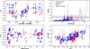 |
Fig. 14 W1 signal of Gl 410 and its periodogram before (red) and after (blue) our filtering technique. For this star, the periodogram of the filtered W1 has been obtained by removing a cubic trend (the blue full line). The original periodogram of the filtered data is still visible (dotted line). |
6.5 GI 410
Before the filtering process, the W1 signal of Gl 410 appears to be contaminated by tellurics with a clear dependence on BERV (especially for BERV <−15 km s−1), and dominant modulations at ∼ 1 yr, as visible in red in Fig. 14 with a log FAP of −34.4. There is no direct correlation between the initial W1 and 〈B〉 (R = 0.21).
The application of our filtering technique led to the production of the PaCMAP map displayed in Fig. C.2, from which we have preselected 660 lines labeled as “active” and 475 as “telluric-polluted” to serve as a training set for the SVM. The SVM delineation so found (Fig. C.2), isolates 3730 lines in the area dominated by the telluric pollution (∼ 25% of the lines considered). The filtered W1, recomputed with wPCA on the remaining lines, is cleared from telluric contamination and no dependencies with the BERV was found (visible in blue in Fig. 14). The filtered W1 signal do correlates with the small-scale magnetic field with a Pearson-R score of 0.80. The global evolution of this signal is similar to the one noted in the small-scale magnetic field with a minimum within 2021A and 2022B resulting in a dominating ∼ 900 d signal in its periodogram. Once detrended using a cubic function, the periodogram of the obtained signal shows that the dominating periodic modulation corresponds to the rotation period of the star, measured here at 14.0 d, coherent with the values in the literature (Hébrard et al. 2016; Donati et al. 2023; Fouqué et al. 2023; Cristofari et al., in prep.).
On all the targets, we demonstrated the efficiency of our method that filters the telluric contamination and retrieves an activity signal in W1 that correlates with 〈B〉 with a correlation coefficient greater or equal to 0.80. This filtering process is always preferable than looking at further principal vectors of the wPCA and needs no other a priori knowledge on the activity signal than its expected modulation period. A summary of all the results of this filtering process on all these stars and the model can be found in Table 2.
6.6 Activity cluster and lines of interest
Looking at the AU Mic, EV Lac and GJ1289 projection maps of per-line dLW periodogram obtained using PaCMAP – Figs. 7, 9 and 11 – we can see clusters that are noticeably emerging from the main cluster of their respective maps. Those lines were, of course, all preselected in the activity group when applying our filtering technique. Unlike the other preselected lines in this group, the activity signal is not only dominant one, but also the only one to strongly influence their width variations, as predicted using simulated data, and they are not affected by any other spurious signals of any origin. In the case of AU Mic, the cluster is composed of 162 lines whose width exclusively varies at the rotation period according to their dLW periodogram. Among them, some lines appear twice because of overlapping orders. The AU Mic's activity cluster is then composed of 131 different lines. Similarly, the activity cluster of EV Lac contains 88 occurrences of 82 different lines whose dLW solely varying with Prot. There is significant overlap as well between the lines found in the two stars. Half of the 82 individual lines of the EV Lac's cluster are also in AU Mic's one. In GJ1289 as well we notice a separated cluster that contains 27 occurrences of 24 individual lines with closely aligned dLW periodograms that contains mainly activity signatures, with only one of them previously recorded in the list composed of lines from AU Mic and EV Lac's activity cluster. In total, without the overlap between targets and orders, we obtain a list of 201 individual lines that are interesting to monitor the activity since their differential line width varies strongly and exclusively with the activity. In Fig. 15 are displayed some of the properties of these lines such as their wavelength, their dLW amplitude at the rotation period of the star considered or their Landé factor for the line we identified. The complete table of properties of this line list is available in electronic form at the CDS. The identification process relies on the wavelengths and depths extracted from the VALD database of stellar lines for the temperature of 3500 K. Some lines remain unidentified due to either having no corresponding match or multiple matches in the mask spectrum. Since the lines of those clusters seem to only encapsulate stellar activity, they could be promising for future study, especially of magnetic variations.
Those lines also seem to encapsulate the activity for the other targets. If no similar activity cluster is found for the other stars, the lines previously identified using AU Mic, EV Lac & GJ1289 are more likely to be found in the areas dominated by the activity as defined by the SVM. For example, for GJ1286, 241 occurrences of this line list are considered for the study. As seen previously, according to the SVM (with the additional weighting), the activity dominated area, where the wPCA is recomputed after filtering, contains 83% of the line. Thus, when randomly picking 241 lines the expectation is that 180 of these lines falls into the activity dominated area. However for that list of 241 lines, 198 are in this area which is an over-representation that deviates by 2.6 σ according to the hyper-geometrical distribution. The probability of such an over-representation occurring randomly is less than 0.3%. This over-representation is also confirmed in Gl 410. For this star, the occurrences of the lines derived from the activity clusters of AU Mic, EV Lac and GJ1289 are predominantly found in the activity areas defined by the SVM. This over-representation deviates by 3.8 σ with a probability of occurring randomly of 4 × 10⁻⁵.
Our results strongly suggest that a majority of the lines in this list are associated with the magnetic activity and may serve as interesting candidates for future studies aimed at monitoring the magnetic field. This is supported by their tendency to form distinct clusters in the most active star of our sample and their over-representation in the activity-dominated areas of the other stars. A closer examination of this line list reveal that all the lines exhibit strong modulation of dLW at the rotational period, even those with the smallest Landé factor. The distribution of their Landé factor do not differ significantly from the distribution in the stellar line mask used to identify them and might then be primarily inferred by temperature effects induced by the stellar spots (Huélamo et al. 2008; Boisse et al. 2011; Reiners et al. 2013; Carmona et al. 2023; Larue et al., in prep.).
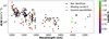 |
Fig. 15 Properties of the lines isolated in the AU Mic, EV Lac, and GJ1289 clusters. The color represents the Landé factor. If the line has not been identified or if no information about its Landé factor has been found, its color has been turn into black, gray, or white. |
7 Conclusion and discussions
We have confirmed W1, introduced by Donati et al. (2023) and defined as the first principal component of the dLW that traces changes in the width of stellar lines, as a robust activity indicator. We obtained the W1 time series from the LBL analysis of five M dwarfs with various levels of stellar magnetic activity, spectral types, and rotation periods – namely AU Mic, EV Lac, GJ1286, GJ1289 and Gl 410 – observed in the NIR with SPIRou.
The small-scale magnetic field is one of the best indicators of RV activity jitter in the case of the Sun (Haywood et al. 2016; Haywood et al. 2022), Sun-like stars (Haywood et al. 2022), and the M dwarf AU Mic (Donati et al. 2023). However, retrieving its time series on M dwarfs is a complicated process. Paul23b relies on relatively high S/N measurements of the spectra (Cristofari et al. 2023) and can be expensive regarding computational time. In this paper, we confirm that W1 can serve as a robust proxy for the small-scale magnetic field for M dwarf stars beyond AU Mic (Donati et al. 2023) by applying some filtering steps, if necessary. The W1 signal correlates with the small scale magnetic field for stars with a strong magnetic activity, such as AU Mic (as already demonstrated in Donati et al. 2023) and EV Lac, as well as for moderately active stars, for example GJ1289, GJ1286, and Gl 410. However, for targets other than AU Mic, the lower S/N or the fainter activity signal complicate the analysis. Indeed, the wPCA is dominated by a signal inferred by residual telluric contamination. To deal with it, we built a filtering technique involving the DR algorithm PaCMAP (Wang et al. 2021) and a SVM (Cortes & Vapnik 1995). Our approach enables a refined wPCA computation using only the per-line dLW measurements from the lines primarily affected by stellar activity. As a result, the first principal vector, W1, which was initially contaminated by telluric signals, is not only effectively cleared of telluric signals, but it also becomes systematically and strongly correlated with the small-scale magnetic field (R ≥0.80), which is notoriously challenging to compute for M dwarfs. Since this method is data driven, we employed a model to assess its viability on a controlled simulation. Forthcoming work will involve applying W1 directly as an activity indicator to model and remove the stellar RV jitter using tools such as multidimensional Gaussian processes (Barragán et al. 2022; Camacho et al. 2023) and comparing it to other activity indicators derived from SPIRou spectra.
We observed that for the star GJ1286, our filtering technique performs less optimally. To improve its effectiveness in distinguishing and excluding telluric contamination, we adjusted the weighting coefficients of the SVM. This star has the longest rotation period in our sample, which is relatively close to the 1/2 yr harmonic. Additionally, it is of the latest type, is the faintest, and had the lowest S/N spectra among our targets. This case highlights the technical challenges our filtering technique encounters for slower rotators, particularly when their rotational periods align with a telluric signature, such as 1 yr and its harmonics. We were able to successfully filter the W1 signal of GJ1286 despite its rotation period being close to 1/2 year. In this case, the stellar activity does not show modulations at its rotation period but rather at its second harmonic, as seen in its small-scale magnetic field. This is why we considered both Prot and Prot/2 in the preselection of active lines. Additionally, the dimensionality reduction algorithm PaCMAP proved to be helpful by preserving the global structure of the input data (Wang et al. 2021) – including overall trends – which facilitated the separation of the telluric contamination. Even in this peculiar configuration, we were able to remove the telluric contamination from W1, and the W1 signal now correlate strongly with the small-scale magnetic field. It is important to note that the method relies on the input rotation period to guide the selection of activity-sensitive lines. If the period is inaccurate, the filtering may become less effective or biased. To account for uncertainties, the ± 5% range used to preselect activity lines can be adjusted as needed. However, widening this range increases the risk of including unrelated signals, which may complicate the analysis. In many cases, even with moderate uncertainty on the period, the method can still help isolate and remove telluric contamination and retain meaningful activity signals. The most limiting situations occur when the rotation period is close to strong telluric signals, as illustrated by the case of GJ 1286. While careful consideration is needed, especially in such configurations, the method remains a useful approach to disentangle overlapping signals in RV data.
Additionally, an outcome of the filtering process was the identification of 201 individual lines that specifically capture magnetic activity through variations in their line width. These lines form distinct activity clusters in the PaCMAP projection for the star with the strongest magnetic activity and are significantly overrepresented in the activity-dominated areas identified by the SVM for the other stars. We were able to identify some of them using a mask of stellar lines extracted from the VALD database for stars in this range of temperature. Further investigation will be needed to assess the line list provided. However, our findings indicate that these lines are predominantly influenced by activity signals, and most of them are likely to be useful for monitoring the magnetic field of M dwarf stars.
In this paper, we have presented a framework that uses a DR algorithm and SVM to classify LBL measurements of per-line dLW time series based on two known periodicities: the rotational modulation caused by stellar activity, which we aimed to extract, and telluric contamination, which we sought to remove. The ability to disentangle signals based on their periodicities has broad applications in exoplanetology, is perfectly suited for the LBL framework, and could be extend to various instruments and targets. While we applied this method on per-line dLW measurements to decontaminate their principal vector, it can be easily extended to other activity indicators produced by LBL (Artigau et al. 2022; Artigau et al. 2024), or even to LBL RVs. More generally, this approach is well suited to any problem where a known signal needs to be suppressed to reveal another targeted signal. For instance, in RV follow-up studies, this technique could be used to identify and exclude spectral lines significantly impacted by stellar activity or telluric contamination, which would allow one to isolate lines primarily influenced by planetary signals and thus reduce RV jitter and potentially uncover additional planets within a system.
Data availability
The data used in this work were recorded in the context of the SPIRou Legacy Survey (SLS) and SPICE large program, and are available to the public at the Canadian Astronomy Data Center9 (CADC) one year after completion of the program, i.e. since February 2024 for SLS data and August 2025 for the SPICE data. PI and DDT data are also available to the public.
The codes used for the filtering process, the simulation, and the PSD analysis can be found on the author's GitHub page: https://github.com/Paul-Charpentier/SPCAndie/tree/main
The full list of identified lines described in Sect. 6.6 is available in its full version at the CDS via https://cdsarc.cds.unistra.fr/viz-bin/cat/J/A+A/701/A17.
Acknowledgements
This project received funding from the European Research Council (ERC) under the H2020 research & innovation program (grant #740651 NewWorlds). Our work is based on observations obtained at the Canada-France-Hawaii Telescope (CFHT), which is operated by the National Research Council (NRC) of Canada, the Institut National des Sciences de l'Univers of the Centre National de la Recherche Scientifique (INSU/CNRS) of France, and the University of Hawaii. The CFHT observations were performed with great care and respect from the summit of Maunakea, a location of immense cultural and historical significance. We wish to acknowledge the significant cultural role and reverence that the summit of Maunakea has always held within the indigenous Hawaiian community. We are incredibly fortunate to have had the opportunity to conduct observations from this mountain, which plays a vital part in our study. This study has been partially supported through the grant EUR TESS No. ANR-18-EURE-0018 in the framework of the Programme des Investissements d'Avenir. We thank the anonymous referee for their comments and suggestions, which helped to improve the clarity and quality of this manuscript.
Appendix A Modeling the observed spectral noise
In the toy model developed in Section 4, our aim is to inject a spectral noise that corresponds to the real spectral noise that is present in the SPIRou spectra. This noise is mainly photon noise, which is a white, spectrally uncorrelated, noise. However, as mentioned in the main body of this article, the processing of the APERO reduction of the raw spectra implies corrections and interpolations that may alter the general properties of this noise. The light transiting through the 35 m of fiber might also have generated some modal noise (Blind 2022) albeit such a noise has not been measured for SPIRou fibers (Micheau et al. 2012; Micheau et al. 2018). The first objective is to measure this noise. From APERO corrected spectra of EV Lac, we standardize, unblaze, and realign the pixels to correct for the BERV and finally subtract them by a template that is the averaged spectra. Here, we are working on a specific range of wavelengths of 50 nm between 2170−2220 nm that is within the spectral order 44 of the detector which is the one with the best S/N and in which there are almost no big telluric or stellar lines. The resulting spectra are supposed to only contain spectral noise, and we then record their Power Spectral Density (PSD). While the PSD of a white noise is expected to be flat, Fig. A.1 shows that the observed PSD is more complex and globally decreasing. Its slope appears to vary with the frequency. At low frequencies, it decreases mostly 'linearly' (in the log-log scale); it then flattens at mid-range frequencies before decreasing again for higher frequencies, with a sharper decline as the frequency increases. This general behavior is also observed in various other targets of the SLS/SPICE programs.
We then fit the mean PSD profile with a classic power law10 that has the form a/fb for frequencies lower than the cut-off frequency of 1 nm−1 and with a quadratic power law (a/fb−c log f) for higher frequencies than the cut-off frequency of 7 nm−1. The fitted parameters are a=3.42 × 10⁻⁴ and b=0.69 for low frequencies and a=1.77 × 10⁻⁵, b=3.24 and c=0.86 for high frequencies. For mid-range frequencies, between 1 nm−1 and 7 nm−1, we modelize it with a constant line, with a=3.59 × 10⁻⁴, connecting the low and high frequency regime since the PSD seems more or less flat within that range except for correlated structures introduced by the realignment step. We then generated noise from this modeled PSD and used it in our model. In practice, we generated a white noise, filtered it using the defined function, and renormalized it.
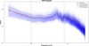 |
Fig. A.1 Power spectral density of the SPIRou spectral noise after APERO corrections and reductions. In blue are every individual spectra while in dashed black is the averaged PSD profile (± its standard deviation in dotted lines). The red dashed, dotted and full lines are the fitted PSD profiles for respectively low, mid and high frequencies. The green vertical lines indicating the cut-off frequencies between those regimes. |
Appendix B Construction details on PaCMAP maps
The Pairwise Controlled Manifold Approximation Projection (PaCMAP, Wang et al. 2021) method is a dimensionality reduction method that can be used for data visualization and cluster analysis. Dimension reduction algorithm transform or project data from a high-dimensional space into a low-dimensional space so that the low-dimensional representation retains the most meaningful properties of the original data, ideally close to its initial dimension. The idea is to attract together in clusters objects with similar properties in the high-dimensional space in the low-dimensional space and reversely repulse objects that are different in the high-dimensional space. This then allows objects to be differentiated into different classifications according to their relative positions in the low-dimensional space (see Part 5.3). Many DR algorithms have been developed for different usage. For example, some of them are focusing on preserving the local structures of the high-dimensional space, such as t-SNE (Van der Maaten & Hinton 2008) and UMAP (McInnes et al. 2018) by strongly repulsing further objects, while some other do conserve the global structure of the high-dimensional space such as TriMAP (Amid & Warmuth 2019) thanks to the involvement of PCA (as we show later) and the dominance of attracting forces within neighbors. PaCMAP consider both of these aspects and is significantly faster than the other mentioned algorithms (See Wang et al. 2021 and Huang et al. 2022 for the complete benchmark). Here is an overview of the algorithm. For the complete description, please refer to Wang et al. (2021).
We considered X as the high-dimensional data matrix on which we apply the dimensional reduction. In the example of our paper, X is a data table of Nlines dLW periodograms sampled on the same period grid of size Nperiods as defined in part 5.2. Let's call Y the low-dimensional matrix. In this paper, we project our data on a 2D map; thus Y has a (Nlines, 2) dimension.
For every line, we construct a set of pairs by sampling nNB nearest neighbors, nMN mid-near pairs and nFP Further pairs from the high-dimensional space X11.
We then initialized Y using a PCA to have a first guess of a map that would conserve the global structure12 (iteration 0 in Fig. B.1)
Then, we iteratively minimized the loss function:
 (B.1)
where d̃ij = ∥yi−yj∥2 + 1 is the distance between two points in the low-dimensional space, Y (offset by 1), and wNB, wMN, wFP are the weights associated with neighbor, mid-near, and further pairs. The weights are evolving with the number of iteration13 as depicted in Fig. B.2. In early iterations, the algorithm focuses on global structure, both neighbors and mid-near pairs are attracted, and the further points are repulsed. Over time, once the global structure is in place, the attractive force on the mid-near pairs decreases, then stabilizes and eventually disappears, leaving the algorithm to refine details of the local structure. 450 iterations are enough for most datasets, including our LBL dLW periodograms, to converge. The evolution of the low-dimensional Y space over the optimization process is visible Fig. B.1.
(B.1)
where d̃ij = ∥yi−yj∥2 + 1 is the distance between two points in the low-dimensional space, Y (offset by 1), and wNB, wMN, wFP are the weights associated with neighbor, mid-near, and further pairs. The weights are evolving with the number of iteration13 as depicted in Fig. B.2. In early iterations, the algorithm focuses on global structure, both neighbors and mid-near pairs are attracted, and the further points are repulsed. Over time, once the global structure is in place, the attractive force on the mid-near pairs decreases, then stabilizes and eventually disappears, leaving the algorithm to refine details of the local structure. 450 iterations are enough for most datasets, including our LBL dLW periodograms, to converge. The evolution of the low-dimensional Y space over the optimization process is visible Fig. B.1.
Thus, we understand that the axes for the 2D map produced do not especially represent anything (except right after the PCA initialization). This is only data visualization. That's why we never display them in this article.
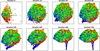 |
Fig. B.1 Illustration of the low-dimensional embedding over the optimization process of PaCMAP on AU Mic's dLW periodograms. |
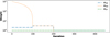 |
Fig. B.2 Evolution of the pair weighting as a function of the number of iterations. |
Appendix C PaCMAP maps and SVM delineation for GJ1286 and GI 410
Figures C.1 and C.2 display the PaCMAP projection and the SVM delineations find for GJ1286 and Gl 410 respectively.
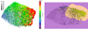 |
Fig. C.1 PaCMAP map of reduced line-by-line dLW periodograms of the star GJ1286 and the optimum separation between the “activity” and the “tellurics” when multiplying all weights of the preselected activity lines by 1.6. |
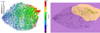 |
Fig. C.2 PaCMAP map of reduced line-by-line dLW periodograms of the star Gl 410 and the optimum separation between the “activity” and the “tellurics.” |
References
- Alvarez, R., & Plez, B., 1998, A&A, 330, 1109 [NASA ADS] [Google Scholar]
- Amid, E., & Warmuth, M. K., 2019, arXiv e-prints [arXiv:1910.00204] [Google Scholar]
- Anglada-Escudé, G., Amado, P. J., Barnes, J., et al. 2016, Nature, 536, 437 [Google Scholar]
- Artigau, É., Astudillo-Defru, N., Delfosse, X.,, et al. 2014, SPIE Conf. Ser., 9149, 914905 [NASA ADS] [Google Scholar]
- Artigau, É., Cadieux, C., Cook, N. J.,, et al. 2022, AJ, 164, 84 [NASA ADS] [CrossRef] [Google Scholar]
- Artigau, É., Cadieux, C., Cook, N. J.,, et al. 2024, AJ, 168, 252 [Google Scholar]
- Banjoko, A. W., Yahya, W. B., Garba, M. K., & Abdulazeez, K. O., 2019, J. Phys.: Conf. Ser., 1366, 012101 [Google Scholar]
- Barragán, O., Aigrain, S., Rajpaul, V. M., & Zicher, N., 2022, MNRAS, 509, 866 [Google Scholar]
- Basant, R., Luque, R., Bean, J. L., et al. 2025, ApJ, 982, L1 [Google Scholar]
- Bellotti, S., Morin, J., Lehmann, L. T., et al. 2024, A&A, 686, A66 [NASA ADS] [CrossRef] [EDP Sciences] [Google Scholar]
- Bertaux, J. L., Lallement, R., Ferron, S., Boonne, C., & Bodichon, R., 2014, A&A, 564, A46 [NASA ADS] [CrossRef] [EDP Sciences] [Google Scholar]
- Blind, N., 2022, SPIE Conf. Ser., 12184, 121844I [Google Scholar]
- Boisse, I., Bouchy, F., Hébrard, G., et al. 2011, A&A, 528, A4 [NASA ADS] [CrossRef] [EDP Sciences] [Google Scholar]
- Bonfils, X., Delfosse, X., Udry, S., et al. 2013, A&A, 549, A109 [NASA ADS] [CrossRef] [EDP Sciences] [Google Scholar]
- Boser, B. E., Guyon, I. M., & Vapnik, V. N., 1992, in Proceedings of the Fifth Annual Workshop on Computational Learning Theory, COLT '92 (New York, NY, USA: Association for Computing Machinery), 144 [Google Scholar]
- Bouchy, F., Pepe, F., & Queloz, D., 2001, A&A, 374, 733 [NASA ADS] [CrossRef] [EDP Sciences] [Google Scholar]
- Camacho, J. D., Faria, J. P., & Viana, P. T. P., 2023, MNRAS, 519, 5439 [NASA ADS] [CrossRef] [Google Scholar]
- Carmona, A., Delfosse, X., Bellotti, S., et al. 2023, A&A, 674, A110 [NASA ADS] [CrossRef] [EDP Sciences] [Google Scholar]
- Carmona, A., Delfosse, X., Ould-Elhkim, M., et al. 2025, A&A, 700, A222 [NASA ADS] [CrossRef] [EDP Sciences] [Google Scholar]
- Chang, Y.-W., Hsieh, C.-J., Chang, K.-W., Ringgaard, M., & Lin, C.-J., 2010, J. Mach. Learn. Res., 11, 1471 [Google Scholar]
- Chen, H., Tian, H., Li, H., et al. 2022, ApJ, 933, 92 [NASA ADS] [CrossRef] [Google Scholar]
- Cook, N. J., Artigau, É., Doyon, R.,, et al. 2022, PASP, 134, 114509 [NASA ADS] [CrossRef] [Google Scholar]
- Cortes, C., & Vapnik, V., 1995, Mach. Learn., 20, 273 [Google Scholar]
- Cretignier, M., Dumusque, X., Allart, R., Pepe, F., & Lovis, C., 2020, A&A, 633, A76 [NASA ADS] [CrossRef] [EDP Sciences] [Google Scholar]
- Cristofari, P. I., Donati, J. F., Masseron, T., et al. 2022, MNRAS, 516, 3802 [NASA ADS] [CrossRef] [Google Scholar]
- Cristofari, P. I., Donati, J. F., Moutou, C., et al. 2023, MNRAS, 526, 5648 [NASA ADS] [CrossRef] [Google Scholar]
- Delchambre, L., 2015, MNRAS, 446, 3545 [NASA ADS] [CrossRef] [Google Scholar]
- Díez Alonso, E., Caballero, J. A., Montes, D.,, et al. 2019, A&A, 621, A126 [NASA ADS] [CrossRef] [EDP Sciences] [Google Scholar]
- Donati, J. F., & Brown, S. F., 1997, A&A, 326, 1135 [Google Scholar]
- Donati, J. F., Kouach, D., Moutou, C., et al. 2020, MNRAS, 498, 5684 [Google Scholar]
- Donati, J. F., Lehmann, L. T., Cristofari, P. I., et al. 2023, MNRAS, 525, 2015 [CrossRef] [Google Scholar]
- Dressing, C. D., & Charbonneau, D., 2015, ApJ, 807, 45 [Google Scholar]
- Dumusque, X., 2018, A&A, 620, A47 [NASA ADS] [CrossRef] [EDP Sciences] [Google Scholar]
- Faria, J. P., Suárez Mascareño, A., Figueira, P., et al. 2022, A&A, 658, A115 [NASA ADS] [CrossRef] [EDP Sciences] [Google Scholar]
- Fischer, D. A., Anglada-Escude, G., Arriagada, P., et al. 2016, PASP, 128, 066001 [Google Scholar]
- Folsom, C. P., Petit, P., Bouvier, J., et al. 2016, MNRAS, 457, 580 [Google Scholar]
- Fouqué, P., Moutou, C., Malo, L., et al. 2018, MNRAS, 475, 1960 [Google Scholar]
- Fouqué, P., Martioli, E., Donati, J. F., et al. 2023, A&A, 672, A52 [NASA ADS] [CrossRef] [EDP Sciences] [Google Scholar]
- Gaia Collaboration (Brown, A. G. A., et al.,) 2018, A&A, 616, A1 [NASA ADS] [CrossRef] [EDP Sciences] [Google Scholar]
- Gaidos, E., Mann, A. W., Kraus, A. L., & Ireland, M., 2016, MNRAS, 457, 2877 [Google Scholar]
- Giacobbe, P., Benedetto, M., Damasso, M., et al. 2020, MNRAS, 491, 5216 [Google Scholar]
- Gilbert, E. A., Barclay, T., Quintana, E. V., et al. 2022, AJ, 163, 147 [NASA ADS] [CrossRef] [Google Scholar]
- Gustafsson, B., Edvardsson, B., Eriksson, K., et al. 2008, A&A, 486, 951 [NASA ADS] [CrossRef] [EDP Sciences] [Google Scholar]
- Haywood, R. D., Collier Cameron, A., Queloz, D., et al. 2014, MNRAS, 443, 2517 [Google Scholar]
- Haywood, R. D., Collier Cameron, A., Unruh, Y. C., et al. 2016, MNRAS, 457, 3637 [Google Scholar]
- Haywood, R. D., Milbourne, T. W., Saar, S. H., et al. 2022, ApJ, 935, 6 [NASA ADS] [CrossRef] [Google Scholar]
- Hébrard, É. M., Donati, J. F., Delfosse, X.,, et al. 2014, MNRAS, 443, 2599 [CrossRef] [Google Scholar]
- Hébrard, É. M., Donati, J. F., Delfosse, X.,, et al. 2016, MNRAS, 461, 1465 [CrossRef] [Google Scholar]
- Hsu, D. C., Ford, E. B., & Terrien, R., 2020, MNRAS, 498, 2249 [Google Scholar]
- Huang, H., Wang, Y., Rudin, C., & Browne, E. P., 2022, Commun. Biol., 5, 719 [Google Scholar]
- Huélamo, N., Figueira, P., Bonfils, X., et al. 2008, A&A, 489, L9 [NASA ADS] [CrossRef] [EDP Sciences] [Google Scholar]
- Klein, B., Donati, J.-F., Moutou, C., et al. 2021, MNRAS, 502, 188 [Google Scholar]
- Kochukhov, O., 2021, A&A Rev., 29, 1 [NASA ADS] [CrossRef] [Google Scholar]
- Lagrange, A. M., Meunier, N., Desort, M., & Malbet, F., 2011, A&A, 528, L9 [NASA ADS] [CrossRef] [EDP Sciences] [Google Scholar]
- Landstreet, J. D., 1988, ApJ, 326, 967 [Google Scholar]
- Latouf, N., Wang, S. X., Cale, B., & Plavchan, P., 2022, AJ, 164, 212 [NASA ADS] [CrossRef] [Google Scholar]
- Lehmann, L. T., Donati, J. F., Fouqué, P., et al. 2024, MNRAS, 527, 4330 [Google Scholar]
- Mamajek, E. E., & Bell, C. P. M., 2014, MNRAS, 445, 2169 [Google Scholar]
- Martioli, E., Hébrard, G., Correia, A. C. M., Laskar, J., & Lecavelier des Etangs, A. 2021, A&A, 649, A177 [NASA ADS] [CrossRef] [EDP Sciences] [Google Scholar]
- Mayor, M., & Queloz, D., 1995, Nature, 378, 355 [Google Scholar]
- McInnes, L., Healy, J., & Melville, J., 2018, arXiv e-prints [arXiv:1802.03426] [Google Scholar]
- Meunier, N., & Lagrange, A. M., 2019, A&A, 625, L6 [NASA ADS] [CrossRef] [EDP Sciences] [Google Scholar]
- Meunier, N., Desort, M., & Lagrange, A. M., 2010, A&A, 512, A39 [NASA ADS] [CrossRef] [EDP Sciences] [Google Scholar]
- Micheau, Y., Bouchy, F., Pepe, F., et al. 2012, SPIE Conf. Ser., 8446, 84462R [Google Scholar]
- Micheau, Y., Kouach, D., Donati, J.-F., et al. 2018, SPIE Conf. Ser., 10702, 107025R [NASA ADS] [Google Scholar]
- Morin, J., Donati, J. F., Petit, P., et al. 2008, MNRAS, 390, 567 [Google Scholar]
- Moutou, C., Fares, R., & Donati, J.-F., 2018, in Handbook of Exoplanets, eds. H. J. Deeg & J. A. Belmonte, 21 [Google Scholar]
- Moutou, C., Delfosse, X., Petit, A. C., et al. 2023, A&A, 678, A207 [NASA ADS] [CrossRef] [EDP Sciences] [Google Scholar]
- Moutou, C., Ould-Elhkim, M., Donati, J. F., et al. 2024, A&A, 688, A196 [NASA ADS] [CrossRef] [EDP Sciences] [Google Scholar]
- Muheki, P., Guenther, E. W., Mutabazi, T., & Jurua, E., 2020, MNRAS, 499, 5047 [NASA ADS] [CrossRef] [Google Scholar]
- Newton, E. R., Mondrik, N., Irwin, J., Winters, J. G., & Charbonneau, D., 2018, AJ, 156, 217 [Google Scholar]
- Ould-Elhkim, M., Moutou, C., Donati, J. F., et al. 2023, A&A, 675, A187 [NASA ADS] [CrossRef] [EDP Sciences] [Google Scholar]
- Paudel, R. R., Barclay, T., Schlieder, J. E., et al. 2021, ApJ, 922, 31 [NASA ADS] [CrossRef] [Google Scholar]
- Pepe, F., Cristiani, S., Rebolo, R., et al. 2021, A&A, 645, A96 [NASA ADS] [CrossRef] [EDP Sciences] [Google Scholar]
- Plavchan, P., Barclay, T., Gagné, J., et al. 2020, Nature, 582, 497 [Google Scholar]
- Plez, B., 2012, Turbospectrum: Code for spectral synthesis, Astrophysics Source Code Library [record ascl:1205.004] [Google Scholar]
- Reiners, A., 2012, Living Rev. Sol. Phys., 9, 1 [Google Scholar]
- Reiners, A., Shulyak, D., Anglada-Escudé, G., et al. 2013, A&A, 552, A103 [NASA ADS] [CrossRef] [EDP Sciences] [Google Scholar]
- Reiners, A., Zechmeister, M., Caballero, J. A., et al. 2018, A&A, 612, A49 [NASA ADS] [CrossRef] [EDP Sciences] [Google Scholar]
- Reylé, C., Jardine, K., Fouqué, P., et al. 2021, A&A, 650, A201 [Google Scholar]
- Sabotta, S., Schlecker, M., Chaturvedi, P., et al. 2021, A&A, 653, A114 [NASA ADS] [CrossRef] [EDP Sciences] [Google Scholar]
- Sameshima, H., Matsunaga, N., Kobayashi, N., et al. 2018, PASP, 130, 074502 [NASA ADS] [CrossRef] [Google Scholar]
- Schöfer, P., Jeffers, S. V., Reiners, A., et al. 2022, A&A, 663, A68 [NASA ADS] [CrossRef] [EDP Sciences] [Google Scholar]
- Suárez Mascareño, A., González-Álvarez, E., Zapatero Osorio, M. R., et al. 2023, A&A, 670, A5 [NASA ADS] [CrossRef] [EDP Sciences] [Google Scholar]
- Szabó, G. M., Gandolfi, D., Brandeker, A., et al. 2021, A&A, 654, A159 [NASA ADS] [CrossRef] [EDP Sciences] [Google Scholar]
- Szabó, G. M., Garai, Z., Brandeker, A., et al. 2022, A&A, 659, L7 [NASA ADS] [CrossRef] [EDP Sciences] [Google Scholar]
- Ulmer-Moll, S., Figueira, P., Neal, J. J., Santos, N. C., & Bonnefoy, M., 2019, A&A, 621, A79 [NASA ADS] [CrossRef] [EDP Sciences] [Google Scholar]
- Van der Maaten, L., & Hinton, G., 2008, J. Mach. Learn. Res., 9 [Google Scholar]
- Wade, G. A., Bagnulo, S., Kochukhov, O., et al. 2001, A&A, 374, 265 [NASA ADS] [CrossRef] [EDP Sciences] [Google Scholar]
- Wang, Y., Huang, H., Rudin, C., et al. 2021, J. Mach. Learn. Res., 22, 1 [Google Scholar]
- Wang, S. X., Latouf, N., Plavchan, P., et al. 2022, AJ, 164, 211 [NASA ADS] [CrossRef] [Google Scholar]
- Wattenberg, M., Viégas, F., & Johnson, I., 2016, Distill [Google Scholar]
- Wittrock, J. M., Plavchan, P. P., Cale, B. L., et al. 2023, AJ, 166, 232 [NASA ADS] [CrossRef] [Google Scholar]
- Zechmeister, M., & Kürster, M., 2009, A&A, 496, 577 [CrossRef] [EDP Sciences] [Google Scholar]
- Zechmeister, M., Reiners, A., Amado, P. J., et al. 2018, A&A, 609, A12 [NASA ADS] [CrossRef] [EDP Sciences] [Google Scholar]
Infra-Red Spectropolarimeter in English.
Program ID P40 in semesters 19A to 22A.
Program ID P45 from semesters 22B to 24A.
In the LBL framework, a line is the domain between two local maxima (Artigau et al. 2022).
The Zeeman effect describes the splitting of the energy levels, and thus, spectral lines into multiple components under the influence of a magnetic field, which often appear as a broadening of the observed line when the components are unresolved.
The power law is the classic PSD shape of colored noises where the exponent b determine the color (White → b=0; Red (or Brownian) → b=2; etc.)
The pairs are sampled as following:
The Neighbors Pairs (nNB) are sampled within a scaled distance  where σi is the average distance between the line i and its Euclidean nearest fourth to sixth neighbors in the high-dimensional space X.
The Mid-Near pairs (nMN) are sampled by selecting the second closest of six random observations in the X space.
Further Pairs (nFP) are sampled from all the non-neighbors lines.
By default in the algorithm, the ratio between nNB, nMN and nFP is nNB = 2 nMN = 0.5 nFP.
One could initialize Y by placing the lines randomly in the map as well but it converge more quickly with a first guess of the global structure using PCA.
For the details, in the first 100 iterations (the early exaggeration stage), we set  decreases linearly from 1000 to 3); wFP = 1. In the second stage (the next 100 iterations), wNB = 3; wMN = 3; wFP = 1. Then for the latest iterations, wNB = 1; wMN = 0; wFP = 1.
All Tables
All Figures
|
Fig. 1 Small-scale magnetic field measurements from ZeeTurbo (Cristofari et al. 2023) using SPIRou spectra for AU Mic, EV Lac, GJ1289, and Gl 410, along with their periodograms. The black horizontal lines (solid, dashed, dotted) indicate false alarm probabilities of 10%, 1%, and 0.1%. The vertical blue dashed line marks the literature rotation period. The gray curve represents the window function, illustrating time sampling effects. |
| In the text | |
|
Fig. 2 Small-scale magnetic field measurements of GJ1286 along with its periodogram. In this case the periodogram has been obtained by first removing a quadratic trend. The periodogram of the original data is still visible (purple dotted lines). The dashed vertical line indicates the second harmonic of the rotation period while the other vertical and horizontal lines were already presented in Fig. 1. |
| In the text | |
|
Fig. 3 W1 signal of the simulated dataset before (red) and after (blue) our filtering technique. The left panel is the time series, the middle panel is its LS-periodogram, and the right panel is W1 as a function of the BERV. The gray curve represents the window function, illustrating time sampling effects. |
| In the text | |
|
Fig. 4 PaCMAP map of reduced dLW periodograms of the simulated data. The color map indicates the period in days of the strongest peak in the periodogram of that line. |
| In the text | |
|
Fig. 5 Support vector machine separation of the output PaCMAP map. The SVM has been fed using two clouds of points corresponding to lines identified as telluric contaminated (yellow points) or sensitive to the activity (purple point). The SVM has identified their two relative areas. |
| In the text | |
|
Fig. 6 Top left: W1 time series of AU Mic before (red) and after (blue) our filtering technique. Top right: the periodogram of this time series. Bottom left: W1 signal of AU Mic as a function of the BERV. Bottom right: W1 signal of AU Mic as a function of the small-scale magnetic field, <B>. |
| In the text | |
|
Fig. 7 PaCMAP map of reduced LBL dLW periodograms of the star AU Mic. The color map indicates the period in days of the strongest peak in the periodogram of that line, while the size of the point indicates its relative power. |
| In the text | |
|
Fig. 8 W1 signal of EV Lac before (red) and after (blue) our filtering technique. The panels are the same as Fig. 6. |
| In the text | |
|
Fig. 9 Left panel: PaCMAP map of reduced line-by-line dLW periodograms of the star EV Lac. The color map indicates the period in days of the strongest peak in the periodogram of that line. Right panel: optimum separation between the “activity” and the “tellurics.” The size of the points represents the log FAP of the dominant periodic signal. |
| In the text | |
|
Fig. 10 W1 signal of GJ1289 before (red) and after (blue) our filtering technique. Panels are the same as in Fig. 6. |
| In the text | |
|
Fig. 11 PaCMAP map of reduced LBL dLW periodograms of the star GJ1289 and the optimum separation between the “activity” and the “tellurics.” |
| In the text | |
|
Fig. 12 W1 signal of GJ1286 before (red) and after (blue) our filtering technique. Panels are the same as in Fig. 6. The periodogram of this figure was obtained by removing a quadratic trend from the filtered W1 beforehand (visible as a blue full line). The original periodogram of the filtered data is still visible (dotted line). |
| In the text | |
|
Fig. 13 Fraction of lines kept after filtering (blue) and Correlation between the small-scale magnetic field signal and the filtered W1 (red) as a function of the activity class additional relative weighting while performing the SVM for the star GJ1286. The green vertical line represents the weighting ratio chosen for the SVM. |
| In the text | |
|
Fig. 14 W1 signal of Gl 410 and its periodogram before (red) and after (blue) our filtering technique. For this star, the periodogram of the filtered W1 has been obtained by removing a cubic trend (the blue full line). The original periodogram of the filtered data is still visible (dotted line). |
| In the text | |
|
Fig. 15 Properties of the lines isolated in the AU Mic, EV Lac, and GJ1289 clusters. The color represents the Landé factor. If the line has not been identified or if no information about its Landé factor has been found, its color has been turn into black, gray, or white. |
| In the text | |
|
Fig. A.1 Power spectral density of the SPIRou spectral noise after APERO corrections and reductions. In blue are every individual spectra while in dashed black is the averaged PSD profile (± its standard deviation in dotted lines). The red dashed, dotted and full lines are the fitted PSD profiles for respectively low, mid and high frequencies. The green vertical lines indicating the cut-off frequencies between those regimes. |
| In the text | |
|
Fig. B.1 Illustration of the low-dimensional embedding over the optimization process of PaCMAP on AU Mic's dLW periodograms. |
| In the text | |
|
Fig. B.2 Evolution of the pair weighting as a function of the number of iterations. |
| In the text | |
|
Fig. C.1 PaCMAP map of reduced line-by-line dLW periodograms of the star GJ1286 and the optimum separation between the “activity” and the “tellurics” when multiplying all weights of the preselected activity lines by 1.6. |
| In the text | |
|
Fig. C.2 PaCMAP map of reduced line-by-line dLW periodograms of the star Gl 410 and the optimum separation between the “activity” and the “tellurics.” |
| In the text | |
Current usage metrics show cumulative count of Article Views (full-text article views including HTML views, PDF and ePub downloads, according to the available data) and Abstracts Views on Vision4Press platform.
Data correspond to usage on the plateform after 2015. The current usage metrics is available 48-96 hours after online publication and is updated daily on week days.
Initial download of the metrics may take a while.