| Issue |
A&A
Volume 701, September 2025
|
|
|---|---|---|
| Article Number | A175 | |
| Number of page(s) | 13 | |
| Section | Interstellar and circumstellar matter | |
| DOI | https://doi.org/10.1051/0004-6361/202555016 | |
| Published online | 15 September 2025 | |
Mid-infrared extinction curve for protostellar envelopes from JWST-detected embedded jet emission: The case of TMC1A
1
Department of Astronomy, University of Virginia,
Charlottesville,
VA
22903,
USA
2
Virginia Institute of Theoretical Astronomy, University of Virginia,
Charlottesville,
VA
22903,
USA
3
Bluedrop Training & Simulation, Inc.,
36 Solutions Drive #300, Halifax,
Nova Scotia
B3S 1N2,
Canada
4
Leiden Observatory, Leiden University,
PO Box 9513,
2300RA
Leiden,
The Netherlands
5
European Southern Observatory,
Karl-Schwarzschild-Strasse 2,
85748
Garching bei München,
Germany
6
Institut de Ciències de l’Espai (ICE-CSIC), Campus UAB,
Can Magrans S/N,
08193
Cerdanyola del Vallès,
Catalonia,
Spain
7
Institut d’Estudis Espacials de Catalunya (IEEC),
c/Gran Capita, 2-4,
08034
Barcelona,
Catalonia,
Spain
8
INAF-Osservatorio Astronomico di Capodimonte,
Salita Moiariello 16,
80131
Napoli,
Italy
9
Chalmers University of Technology, Department of Space, Earth and Environment,
412 96
Gothenburg,
Sweden
10
Max-Planck-Institut für Astronomie,
Königstuhl 17,
69117
Heidelberg,
Germany
11
Dublin Institute for Advanced Studies, DIAS Headquarters,
10 Burlington Road,
D04C932
Dublin,
Ireland
12
National Radio Astronomy Observatory,
520 Edgemont Road,
Charlottesville,
VA
22903,
USA
13
Institute of Astronomy, Department of Physics, National Tsing Hua University,
Hsinchu,
Taiwan
★ Corresponding author.
Received:
2
April
2025
Accepted:
6
July
2025
Abstract
Context. Dust grains are fundamental components of the interstellar medium (ISM), playing a crucial role in star formation as catalysts for chemical reactions and planetary building blocks. Extinction curves can serve as a tool for characterizing dust properties, however mid-infrared (MIR) extinction remains less constrained in protostellar environments. Gas-phase line ratios from embedded protostellar jets offer a spatially resolved method for measuring the extinction from protostellar envelopes, complementing traditional background starlight techniques.
Aims. We aim to derive MIR extinction curves along the lines of sight toward a protostellar jet embedded within an envelope and to assess whether they differ from those inferred from dense molecular clouds.
Methods. We analyzed JWST NIRSpec IFU and MIRI MRS observations, focusing on four locations along the blue-shifted TMC1A jet. After extracting observed [Fe II] line intensities, we modeled the intrinsic line ratios using the Cloudy spectral synthesis code across a range of electron densities and temperatures. By comparing observed near-IR (NIR) and MIR line ratios to intrinsic ratios predicted with Cloudy, we were able to infer the relative extinction between the NIR and MIR wavelengths.
Results. The electron densities (ne) derived from NIR [Fe II] lines range from ~5 × 10⁴ to ~5 × 103 cm−3 along the jet axis at scales ≲350 AU, serving as reference points for comparing the relative NIR and MIR extinction. The derived MIR extinction results display a higher reddening than empirical dark cloud curves at the corresponding ne values and temperatures (from a few 103 to ~104 K) adopted from shock models. While both the electron density and temperature influence the NIR-to-MIR [Fe II] line ratios, the ratios are more strongly dependent on ne over the adopted range. If the MIR emission originates from gas that is less dense and cooler than the NIR-emitting region, the inferred extinction curves remain consistent with background star-derived values.
Conclusions. This study introduces a new line-based method for deriving spatially resolved MIR extinction curves towards embedded protostellar sources exhibiting a bright [Fe II] jet. These results suggest that protostellar envelopes may contain dust with a modified grain size distribution, such as an increased fraction of larger grains (potentially due to grain growth) if the MIR and NIR lines originate from similar regions along the same sight lines. Alternatively, if the grain size distribution has not changed (i.e., there is no grain growth), the MIR lines may trace cooler, less dense gas than the NIR lines along the same sight lines. This method provides a novel approach for studying dust properties in star-forming regions that could be extended to other protostellar systems to refine extinction models in embedded environments.
Key words: stars: jets / dust, extinction / ISM: jets and outflows / infrared: ISM / infrared: stars
© The Authors 2025
 Open Access article, published by EDP Sciences, under the terms of the Creative Commons Attribution License (https://creativecommons.org/licenses/by/4.0), which permits unrestricted use, distribution, and reproduction in any medium, provided the original work is properly cited.
This article is published in open access under the Subscribe to Open model. This email address is being protected from spambots. You need JavaScript enabled to view it. to support open access publication.
1 Introduction
Despite the dust-to-gas mass ratio of 0.01, dust grains are fundamental components of the interstellar medium (ISM), produced during the final stages of stellar evolution and subsequently processed in interstellar environments. These grains act as catalysts for chemical reactions, enabling the formation of complex organic molecules and facilitating key processes essential to star and planet formation (e.g., Johansen et al. 2014; Brügger et al. 2020; Johansen et al. 2021; Boogert et al. 2015; McClure et al. 2023). The earliest stages of planet formation begin with the growth of dust grains, a process that appears to commence early in the star formation sequence (e.g., Drążkowska et al. 2023). While JWST is only beginning to unravel dust grain properties through infrared observations along diffuse Milky Way sight lines (e.g., AV < 2.5; Decleir et al. 2025), the question of how such dust properties endure as a protostar forms to create a dense environment within a collapsing cloud remains unclear.
At millimeter (mm) wavelengths, low spectral index values (referring to the shallow slope of flux density across the mm regime) are often interpreted as evidence for grain growth, suggesting the presence of large grains in the disks and infalling envelopes of the youngest protostars, with ages of ~104−5 years (e.g., Miotello et al. 2014; Galametz et al. 2019; Cacciapuoti et al. 2024). While the sizes of dust grains contributing to this behavior remain less well constrained, models of dust polarization based on radiative alignment torques (RATs) require grains larger than ~10 µm to explain observed polarization levels in protostellar envelopes at mm wavelengths (Valdivia et al. 2019; Le Gouellec et al. 2019).
Across infrared (IR) to ultraviolet (UV) wavelengths, dust grain properties are typically inferred from extinction curves and/or solid-state features of the refractories and/or volatiles. Extinction curves describe how dust grains absorb and scatter light as a function of wavelength, providing a critical tool for probing their composition, size distribution, and processing in astrophysical environments. Observationally, extinction curves are usually derived by measuring the attenuation of stellar photospheric continuum emission along different lines of sight, revealing how dust interacts with radiation in various astro-physical environments (e.g., Cardelli et al. 1989; McClure 2009; Gordon et al. 2009; Fitzpatrick et al. 2019; Gordon et al. 2021, 2023). Theoretically, extinction models connect these observational trends to underlying dust grain populations by adjusting grain size distributions and compositions to match the observed extinction laws (e.g., Weingartner & Draine 2001; Crapsi et al. 2008; Pontoppidan et al. 2024).
Cardelli et al. (1989) introduced a widely adopted UV to near-infrared (NIR) extinction law derived from line-of-sight observations of bright stars with known spectral types, showing that the shape of the extinction curve depends on the total-to-selective extinction ratio (RV = AV/E(B − V)), where AV is the total extinction in the V-band and E(B − V) represents the difference in extinction between the B and V bands. Notably, the observed extinction curves revealed that extinction in the NIR (λ ~ 1−5 µm) appears independent of RV while a larger dependence is found in UV (the so called FUV rise). In the mid-infrared (MIR), McClure (2009) analyzed 5–20 µm Spitzer IRS spectra of background G0-M4 III stars and confirmed that extinction curves derived from stars behind dense dark clouds exhibit higher levels of MIR extinction compared to those behind less opaque clouds, which resemble the diffuse interstellar medium (ISM). The higher extinction regimes correspond to flatter MIR extinction curves relative to the NIR that aligns closely with the RV = 5.5, case B, curve in Weingartner & Draine (2001).
From a modeling perspective, the observed extinction differences relative to optical/IR across lines of sight in the UV (λ < 0.16 µm) and the MIR (5–30 µm) correspond to differences in dust composition, grain size distributions, and the presence of solid-state features such as refractories and volatiles. The RV = 5.5 curve (Case B in Weingartner & Draine 2001) shows higher extinction at λ > 2 µm compared to the RV = 3.1 case, attributed to a decrease in small grains (<0.1 µm) and an increased fraction of larger silicate and carbonaceous grains, resulting in the observed flattening of the extinction curve in the MIR relative to the NIR. This flattening effect is also consistent with the “KP5” extinction curve, which models extinction as a function of wave-length for dense clouds and protostellar envelopes, including the effects from ices (e.g., H2O, CO, and CO2) that introduce sharp opacity features at specific MIR wavelengths (Crapsi et al. 2008; Pontoppidan et al. 2024). The KP5 model assumes a grain size distribution predominantly larger than 0.1 µm, with an upper size limit of 7 µm. This is consistent with the grain size distribution from Weingartner & Draine (2001) and broadly consistent with that measured for two lines of sight within a dense molecular cloud by Dartois et al. (2024), using radiative transfer modeling of the scattering wings of ice features towards two background stars in Chameleon I.
With the empirically derived MIR extinction curve from McClure (2009) showing that denser lines of sight (AK > 1) are more closely aligned with the RV = 5.5 Case B curve, while more diffuse sight lines (AK < 1) resemble the RV = 3.1 curve, there is growing evidence that dust grains grow larger in denser regions. Extending this trend, we consider whether this would lead us to expect an even flatter MIR extinction curve in the denser regions (AK ≳ 2) surrounding a protostar (e.g., as its envelope or disk) where grain size distributions (e.g., due to grain growth) may differ from those inferred in molecular clouds.
As shown in the schematic in Figure 1, one way to probe MIR extinction toward embedded environments is through protostellar outflows, which emit strong atomic and molecular lines that become attenuated by the surrounding dust. Unlike background starlight methods, which require bright sources behind dusty regions, gas emission lines provide a spatially resolved approach to measuring extinction within the envelope itself. These outflows exhibit a hierarchical arrangement of nested structures, commonly traced by species such as [Fe II], H2, and CO, distinguishing between collimated jets, wider molecular outflows, and intermediate-angle disk winds (e.g., Harsono et al. 2023; Pascucci et al. 2025; Tychoniec et al. 2024; Delabrosse et al. 2024; Caratti o Garatti et al. 2024; Le Gouellec et al. 2025).
Gas emission lines from protostellar jets are produced from radiative shocks, where supersonic outflows collide with more slowly moving material, creating sharp transitions at the shock front (e.g., Frank et al. 2014). At this interface, gas is rapidly compressed and heated, initiating a post-shock cooling zone where atomic and molecular species become emissive (e.g., Hollenbach & McKee 1989). For the NIR and MIR [Fe II] lines, shock models predict that these lines become emissive at electron densities ~103−105 cm−3 and temperatures ≳7000 K (Nisini 2008; Giannini et al. 2015a; Koo et al. 2016). It is within this cooling region that atomic and singly ionized species, including forbidden line emission from Fe (i.e., [Fe II]), are collisionally excited. These conditions allow [Fe II] emission to remain strong without being collisionally quenched, making it a reliable tracer of the physical and chemical properties of protostellar jets.
For the purposes of this study, we focus on the Class I protostar TMC1A (IRAS 04365+2535), a ~0.4 M⊙, ~2.7 L⊙ source located in the Taurus Molecular Cloud at a distance of 140 pc (Galli et al. 2019) and disk, viewed at an inclination of ~54º, representing an evolutionary stage approximately 105 years after the onset of star formation (Kristensen et al. 2012; Harsono et al. 2018). Its nested outflow structure consists of a central collimated atomic [Fe II] jet, a wider-angle H2 shell observed with JWST (Harsono et al. 2023; Assani et al. 2024), along with an even broader CO cavity observed with ALMA (Aso et al. 2015; Bjerkeli et al. 2016; Aso et al. 2021). This outflow is embedded within a dense envelope of gas and dust (Di Francesco et al. 2008), which dominates the extinction along the observer’s line of sight. Previous NIR extinction measurements toward TMC1A show that extinction decreases with increasing distance from the protostar, reflecting changes in extinction magnitude (column density) along different sight lines (Assani et al. 2024) also seen in other sources (Erkal et al. 2021; Narang et al. 2023; Delabrosse et al. 2024; Le Gouellec et al. 2024).
To compare relative NIR/MIR extinction along the jet as a probe of changes in the dust grain size distribution (i.e., dust growth) within the envelope, we adopted an approach that combines excitation models with multi-wavelength embedded [Fe II] jet emission line data. We focused on line ratios rather than absolute intensities, as ratios are less sensitive to uncertainties in the emitting surface and source geometry. Emission lines originating from the same upper energy level have traditionally served as robust tools for measuring extinction magnitude, as their intrinsic line ratios depend solely on radiative de-excitation rates, determined by the Einstein A-coefficients, and are independent of physical conditions such as density and temperature (e.g., Nisini 2008; Giannini et al. 2015b). Extending this analysis to include emission lines from different upper energy levels, we leveraged excitation models to predict a range of intrinsic line ratios across a broader wavelength span.
This approach enables us to compute extinction curves from observational line emission data, compare them with the existing extinction laws, and identify potential variations in extinction along different lines of sight. Using JWST NIRSpec IFU and MIRI MRS spectroscopy, we aim to characterize the extinction toward the TMC1A protostellar jet and assess how it compares to extinction laws derived from diffuse and dense cloud environments away from protostars. This study provides a spatially resolved probe of dust properties in a protostellar envelope, offering new insights into how dust evolves during early star formation.
The paper is organized as follows. In Section 2, we describe the JWST observations and data reduction procedures, detailing the processing of NIRSpec IFU and MIRI MRS spectra and the calculation of observed [Fe II] emission line intensities along the jet (Section 2). This is followed by a description of our excitation model for [Fe II] in Section 3. In Section 4, we outline our method for determining relative extinction between gas emission lines, beginning with extinction differences in the simpler case of lines originating from the same upper energy level in the NIR (Section 4.1). We then extend this analysis to the MIR (Section 4.3), using electron density constraints derived from NIR lines (Section 4.2) as a reference for comparing relative extinction. Finally, we consider cases where NIR and MIR lines trace different excitation conditions and examine how these differences influence the derived MIR extinction curves (Section 4.3). In Section 5, we discuss the interpretations of our results in the context of existing extinction laws and dust grain evolution, and we conclude with a summary of our findings in Section 6.
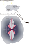 |
Fig. 1 Schematic illustrating extinction sight lines in two contexts. Top panel represents background star extinction studies through diffuse and dense regions of a molecular cloud. Bottom panel (adapted from Fig. 5 of van Dishoeck et al. 2011) shows a forming star embedded in an infalling envelope, with bipolar line-emitting jets carving outflow cavities. The JWST NIRSpec/MIRI field of view probes <1000 AU scales, with the dashed line tracing the line-of-sight path through the dense envelope, where most extinction occurs, toward the inner line emitting jet. |
2 Observations and data reduction
We present NIRSpec IFU and MIRI MRS observations of TMC1A. The NIRSpec data, originally introduced in Harsono et al. (2023) (PID: 2104, PI: Harsono), focused on the [Fe II] lines discussed in Assani et al. (2024). The MIRI MRS observations, presented here for the first time, were obtained on March 4, 2023, as part of the JWST Observations of Young ProtoStars (JOYS) Guaranteed Time Observations (GTO) program (PID: 1290, PI: E. van Dishoeck).
The NIRSpec IFU data, obtained on February 12, 2022, were reprocessed using JWST pipeline v1.11.4 (Bushouse et al. 2023), incorporating updated calibration files (JWST_1123.PMAP) (Greenfield & Miller 2016). This version improved cosmic ray artifact handling, including snowball features, and enhanced flux calibration compared to previous reductions (v1.9.6) used in Harsono et al. (2023). Consistent with prior reductions, we skipped the Stage 3 outlier detection step to avoid excessive flagging of saturated pixels and strong emission lines (Sturm et al. 2023). The final spectral cubes were manually inspected, and problematic spaxels were masked after continuum subtraction and applying signal-to-noise (S/N) thresholds.
The MIRI MRS observations covered a wavelength range of 4.9–28.6 µm with a total integration time of 600 seconds across three sub-bands, each integrated with 36 groups in FASTR1 mode and two dithers optimized for extended emission. The data were processed using JWST pipeline v1.16.1 (Bushouse et al. 2024), with jwst1303.pmap as the calibration reference system. The Detector1Pipeline was applied to the uncal files with default settings to produce detector images, which were subsequently calibrated using the Spec2Pipeline. During this step, the fringe flat was subtracted from the data, residual fringe correction was applied, and a pixel-by-pixel background subtraction was performed using dedicated background detector images. A custom bad-pixel correction was applied using the VIP package (Christiaens et al. 2023). The final data cubes were created using the Spec3Pipeline with the drizzle algorithm (Law et al. 2023), processing each band and channel independently. Due to a telescope mispointing, one of the two dither pointings in channel 1 did not cover the target, so only a single dither was used for that channel, while both dithers were used for all other channels. Background observations were taken immediately prior to the science exposures, using a single dither with 36 groups. The absolute flux calibration uncertainty for the MIRI-MRS observations is estimated to be 5.6% ± 0.7% (Argyriou et al. 2023).
To align the datasets, we determined the protostar’s position by fitting a 2D Gaussian function to the point spread function (PSF) in the NIRSpec and MIRI data. The PSF accounts for diffraction effects caused by JWST’s hexagonal mirror structure. For NIRSpec data, the centroid was calculated at wavelengths greater than 4 µm using the G395H grating, while for MIRI data, centroids were derived independently for each spectral channel. These centroids were then used to spatially align the datasets, ensuring an accurate correspondence with the protostar’s position across a range of wavelengths. After alignment, the data were interpolated onto a common spatial grid using the 0.1″ pixel scale of the NIRSpec IFU data. This resolution oversamples the native MIRI pixel scale (0.196–0.273″), however, it does facilitate a uniform region selection and comparisons across wavelengths.
This analysis focuses on [Fe II] emission lines relevant to our excitation models (Section 3), building on NIR detections reported in Assani et al. (2024) and 4 new MIR [Fe II] lines. In the NIR, we focus on the “a4D” transitions which are detected across the jet and tend to be bright lines (Iλ/I1.644 > 10−2). We omitted lines that are heavily blended; specifically, the 1.748 µm line (blended with H2) and the 4.889 µm line (blended with CO v=1-0). The final dataset includes all “a4D” transition detections, along with the MIRI-detected lines 5.34, 17.99, 24.52 and 25.99 µm. A complete list of these lines, along with their atomic properties, including energy levels, Einstein A-coefficients, and critical densities, is provided in Table A.1.
The observed line intensities were measured at four distinct locations along the blue-shifted axis of the TMC1A jet, focusing on the base of the jet (closer to the protostar) and the intensity peaks previously identified in Assani et al. (2024). These regions are shown as circular, color-coded apertures (diameter 0.7″) overlaid on the moment-0 maps in the top panels of Figure 2. This aperture size exceeds MIRI’s native pixel scale (0.196–0.273″) and approximates instrument’s diffraction limit across the relevant wavelengths (~0.2″ at 5 µm, ~0.7″ at 18 µm, and ~1″ at 26 µm; Law et al. 2023), providing consistent spatial sampling across both NIRSpec and MIRI datasets while minimizing undersampling effects at longer wavelengths.
To extract the line intensities, we summed over each aperture at every spectral channel to produce a 1D spectrum for each region (bottom panels of Figure 2). The line intensities (in erg cm−2 s−1 sr−1) were then computed by integrating the continuum-subtracted spectra in frequency space over ~3–4 channels (corresponding to a velocity range of ~ 150–200 km/s), tailored to encompass the full line while maintaining a consistent integration range across apertures for each line (shaded regions in the bottom panels of Figure 2). The resulting intensities and line ratios (relative to the 1.644 µm line) are reported in Table A.2.
3 The iron line emission model
To model the intrinsic line intensities for [Fe II], we used the CLOUDY spectral synthesis code (Ferland et al. 2017; Chatzikos et al. 2023), which simulates physical and chemical processes in the ionized gas. We set up a single-zone calculation, assuming a uniform density and temperature, over a grid of gas densities and temperatures. We considered radiative decay and collisional processes such as collisional excitation (where free electrons transfer kinetic energy to bound electrons, raising them to higher energy states) and collisional de-excitation (where collisions lower excited atoms to lower energy states). We disabled photoionization and Lyα pumping in our model to remove contributions from radiative excitation, as their influence on [Fe II] emission in jets remains uncertain. Since our technique for inferring extinction curves involves only ratios of [Fe II] lines (controlled by the relative level populations of Fe+), which, in turn, depend only on the density of electrons (the primary collider) and electron temperature Te in K, we followed Verner et al. (1999). Thus, we adopted solar abundances (Grevesse et al. 2010) with a fixed, large Fe abundance (Fe/H = 100). This is a simple technique used to leverage the complex machinery of the CLOUDY code to isolate Fe+ as the species of interest for our analysis, enabling relatively straightforward excitation calculations that depend only on ne and Te.
For this study, we adopted the Verner et al. (1999) [Fe II] spectroscopic dataset, which includes 371 energy levels and spans transitions from the infrared to the ultraviolet. CLOUDY defaults to the Smyth et al. (2019) dataset, which extends to high temperatures for UV and was found to best reproduce the observed UV and optical [Fe II] spectra in the case of an AGN (Sarkar et al. 2021). Differences in the predicted line ratios between datasets arise from uncertainties in Einstein A-coefficients (~30–50%) and collision strength calculations, which influence the final level populations. We find that Verner et al. (1999) reproduces NIR and MIR [Fe II] line ratios with electron density and temperature dependencies consistent with previous non-LTE models used for protostellar jets and Herbig-Haro (HH) objects (e.g., Giannini et al. 2015a; Koo et al. 2016). Collisional strengths in the Verner et al. (1999) dataset for all quartet and sextet transitions were taken from Zhang & Pradhan (1995), with transition rates taken from Quinet et al. (1996). The model estimates a [Fe II] line ratio of I1.257/I1.644 = 1.18, which depends solely on the relative Einstein A-coefficients and transition frequencies, remaining constant across ne and Te. This value is consistent with empirically derived intrinsic ratios of 1.11–1.20 (Giannini et al. 2015b) and is commonly used to estimate extinction magnitudes (Assani et al. 2024; Erkal et al. 2021). Therefore, we adopted the Verner et al. (1999) dataset, since a detailed comparison of infrared dataset performance is beyond the scope of this study.
We adopted a model grid with electron densities (ne ~ 103−106 cm−3) and temperatures (5000–20000 K), based on shock studies indicating that NIR and MIR [Fe II] lines trace low-ionization gas with temperatures above 7000 K and electron densities of ne ~ 103−106 cm−3 (e.g., Nisini 2008; Giannini et al. 2015a; Koo et al. 2016).
4 Differential extinction in NIR and MIR
We compared the observed line ratios with intrinsic ratios from the excitation model to determine extinction differences between the NIR and MIR. The extinction modifies the observed ratio as
 (1)
(1)
where robs is the observed ratio between a NIR or MIR [Fe II] line and the reference line, which in this study is the bright NIR line at 1.644 µm; rmodel is the intrinsic line ratio predicted by the excitation model as a function of ne and Te; and Aλ and Aref represent| the extinction at the observed and reference wavelengths, respectively. Rearranging these terms, we find that the difference in extinction is given by
 (2)
(2)
Since ∆Aλ depends only on robs/rmodel, it directly quantifies the deviation between observed and intrinsic line emission ratios due to differential extinction relative to the reference wavelength.
To compare the derived extinction differences with commonly used extinction curves, we can normalize ∆Aλ by the extinction at the reference wavelength. The normalized extinction ratio is given by
 (3)
(3)
The reference extinction, A1.644, is determined for each aperture along the jet using observed [Fe II] integrated line ratios in the NIR, where commonly used extinction curves show minimal deviation across 1–2 µm (see Section 1). In this study, we used the bright 1.257/1.644 line pair, which arises from the a4D J=7/2 fine-structure state, to calculate A1.644 following Equation (1) in Assani et al. (2024), using β values (β = A1.257/A1.644) from established NIR extinction curves (e.g., Cardelli et al. 1989; Weingartner & Draine 2001; Pontoppidan et al. 2024). The resulting Aı.644 values for each aperture and extinction curve are listed in appendix Table A.3. Starting with the aperture closest to the protostar (Fig. 2, in purple) and moving outward along the jet axis (in yellow), we find Aı.644 = 4.11,4.23,4.00, and 3.57 (corresponding to AV ~ 20−17), with a standard deviation of ~10% between extinction curves and less than 1% variation between RV=3.1 and 5.5 within each curve.
To determine the extinction differences between MIR lines and NIR lines (particularly the 1.644 µm line), we began by establishing a robust reference extinction in the NIR. Here, the reference, A1.644, is required for two key reasons: to normalize differential extinctions for comparisons with commonly used extinction curves and to correct NIR line ratios for extinction so that they can be used to determine the electron density. We first analyzed the extinction differences of NIR lines that share the same upper energy state as the 1.644 µm line (a4D J=7/2), as their intrinsic ratios are independent of physical conditions. We then used our derived A1.644 to compare our extinction differences to NIR extinction curves. This allowed us to derive ∆Aλ at the wavelengths of these lines without uncertainty due to density or temperature effects. Next, we extended our analysis to NIR lines with different upper energy states from that of the 1.644 µm line. After the extinction correction using our derived Aı.644 and existing NIR extinction curves, these lines were used to constrain the electron density (ne). This serves as a key reference for evaluating extinction in the MIR, where both ne and Te influence the intrinsic line ratios. Finally, we compared NIR and MIR extinction properties and assessed how potential differences in the physical conditions (ne, Te) among NIR and MIR emitting regions impact the interpretation of relative NIR/MIR extinction and a comparison to other extinction curves after normalizing With A1.644.
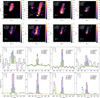 |
Fig. 2 [Fe II] emission lines used in this study and detected with NIRSpec and MIRI, arranged in order of increasing upper energy (EU/k). Top panels: moment-0 maps (in units of erg s−1 cm2 sr−1), constructed by integrating the emission across the frequency range indicated by the shaded regions in the corresponding spectra below. Although integration is performed in frequency space, the x-axis is displayed in velocity (km s−1) for clarity. A 3-sigma threshold is applied. The maps are overlaid with circular, color-coded apertures (0.7″) used consistently throughout this study. Bottom panels: spectra (in units of erg s−1 cm−2 sr−1 Hz−1) extracted from each aperture, with shaded regions highlighting the velocity range used for integration, primarily focusing on blue-shifted emission. Each subplot includes the rest wavelength (λ0), transition and upper energies (∆E, EU), and Einstein-A value for reference. |
4.1 NIR extinction constraints using lines from the same upper energy level
To begin, we validated our line-based extinction method using NIR [Fe II] lines that share the same upper energy level as the 1.644 µm line (a4D J=7/2). These line ratios are insensitive to variations in ne and Te, making them ideal for isolating extinction effects. This provides a clean reference for computing ∆Aλ without any uncertainty from physical conditions, before extending the analysis to lines with different upper states.
The top panel of Figure 3 presents the observed (o, not corrected for extinction) and the modeled (*) line ratios for the a4D J=7/2 upper state across all four jet locations (see Figure 2). The middle panel shows the relative extinction differences (ΔAλ) computed using Equation (2), referenced to the 1.644 µm line. Lines with λ < 1.644 µm (e.g., 1.257, 1.321, and 1.327 µm) exhibit positive extinction differences (ΔA > 0), indicating greater extinction compared to the 1.644 µm line. Conversely, the 1.809 µm line has a negative extinction difference (ΔA < 0), implying lower extinction. This confirms that the extinction curve in the 1–2 µm range has a negative slope, where shorter wavelengths suffer more extinction than longer wave-lengths, consistent with previous NIR extinction studies (e.g., Cardelli et al. 1989; Mathis 1990; Decleir et al. 2022; Gordon et al. 2023). Additionally, the extinction differences exhibit spatial dependence across jet locations, with sight lines that are closer to the protostar (B-purple, F1-blue) showing larger ΔA values at λ < 1.644 µm. This pattern aligns with the finding that total extinction magnitude decreases with distance from the protostar along sight lines directed toward the TMC1A jet, as demonstrated in Assani et al. (2024). Consequently, normalizing by the total extinction at each jet location should account for these differences, revealing a more intrinsic extinction trend across locations.
The negative slope observed in our derived ΔAλ values (middle panel) and the close agreement between our derived βλ values and independent extinction curves and models (bottom panel) confirm the consistency of the extinction curves in the 1.2–1.8 µm range. This consistency reinforces the reliability of using a gas line in this range, such as 1.644 µm, as a reference for measuring relative extinction differences. Moreover, having established a well-constrained extinction correction in the NIR, we can use these NIR lines to probe the physical conditions of the gas emitting these lines, specifically placing constraints on the electron density (ne).
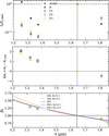 |
Fig. 3 NIR extinction of a4D J=7/2 lines relative to the 1.644 µm line (horizontal and vertical dashed lines.) Top: Observed (‘o’) and modeled (‘*’) line ratios for all four jet locations in this study. Middle: Difference in extinction relative to the 1.644 µm line. Bottom: Derived βλ values, normalized by the extinction at 1.644 µm, which is computed as an average over existing NIR extinction curves. This is compared with empirically determined NIR extinction curves, C89 from Cardelli et al. (1989), and the modeled extinction curves, WD1 by Weingartner & Draine (2001) and KP5 by Pontoppidan et al. (2024). We include RV = 3.1 and RV = 5.5 for applicable curves to illustrate that NIR extinction in the 1.2–1.8 µm range is largely independent of RV and shows minimal differences between independent studies. Dashed lines mark the reference line ratio, extinction difference, and βλ value at 1.644 µm (horizontal) and the wavelength of 1.644 µm (vertical) in all three panels. |
4.2 Electron density constraints from NIR lines
We subsequently extended our analysis to all observed a4D transitions in the NIR to constrain the electron density (ne) at each jet location (see Figure 2). The line ratios of a4D transitions, which originate from states with similar but slightly different upper-level energies (Eupper = 11446−12729 K) and distinct critical densities (ncrit ≈ 4−7 × 104 cm−3 at T = 10000 K), are relatively insensitive to temperature but remain sensitive to electron densities in the 103−5 cm−3 range. This makes them well suited for quantifying ne in the NIR, where the extinction curves are well established.
The derived electron density is not only important in its own right (as a key physical quantity of the NIR line emitting gas in the jet), but it also serves as a starting point for a discussion of the electron density in the MIR line emitting region, which cannot be understood without having firm knowledge of the extinction law for the protostellar envelope where the jet is embedded, which might or might not be the same as that in the NIR line emitting gas. This distinction is particularly relevant as the MIR lines arise from lower excitation levels and may trace gas under different physical conditions (see Section 4.3 below).
Figure 4 presents three examples NIR [Fe II] a4D line ratios used to determine electron density. The predicted line ratios from the [Fe II] model are plotted as a function of electron density across temperatures from 5000 to 20000 K. Observed ratios (circles) and extinction-corrected ratios (squares) are shown with uncertainties. We adopted a constant ~15% uncertainty in extinction for simplicity, consistent with the typical deviations between NIR extinction curves (see Table A.3) and uncertainties in the Einstein A-values (Giannini et al. 2015b), which result in larger uncertainties for the corrected ratios than for the observed ones. Electron density uncertainties primarily arise from (1) uncertainty in the intrinsic line ratios, broadening the possible ne range by approximately a factor of two; and (2) temperature-dependent differences in electron density for a given ratio, which are typically small (<5%).
Near the protostar, electron density estimates approach the critical density (ncrit) of these transitions. Since line ratios become insensitive to the density at ne ≳ ncrit due to thermalization effects (as the gas approaches LTE conditions), constraining electron densities in such regions becomes increasingly uncertain. As a result, the density estimates in the bright region (B-purple) should be interpreted as lower limits. Further from the protostar, intensity ratios relative to the 1.644 µm line are lower, leading to consistently lower and well-constrained electron density estimates.
Across 13 NIR a4D line ratios, electron density estimates remain internally consistent, with differences limited to a factor of ~2 at each jet location (see Table A.4). The results show a clear trend of decreasing electron density along the jet axis:  (knot B-purple), (2.4 + 0.6) × 104 cm−3 (F1-blue), (1.5 + 0.5) × 104 cm−3 (F2-green), and (8.0 + 3.0) × 103 cm−3 (F3-yellow). While uncertainties in adjacent regions overlap in some cases, the overall trend of decreasing electron density with distance from the protostar remains robust. The electron density drops between the bright region (B) and the third peak (F3) exceeds observational uncertainties in most ratios, further reinforcing this trend.
Once the electron density has been determined using NIR [Fe II] gas lines at each jet location, we can use these values as reference points to assess relative extinction between the NIR and MIR along each line of sight toward the TMC1A jet.
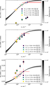 |
Fig. 4 Examples of density-sensitive NIR line ratios, where the CLOUDY model predictions are shown as solid lines shaded by temperature. Observed line ratios with uncertainties are represented by circles, while extinction-corrected ratios are shown as squares color-coded by jet location (see Fig. 2). The extinction-corrected ratio, accounting for uncertainties, determines the electron density from the model, aligning with the x-axis position of both observed and corrected ratios. Top: shorter-wavelength line is more affected by extinction, leading to an increased ratio after correction. Middle: line ratio with similar rest wavelengths, minimally affected by extinction, where the observed ratio closely matches the expected electron density. Bottom: longer wavelength line that is less affected by extinction and causes the ratio to decrease after correction. Following extinction correction using established NIR curves (Section 4.1), all corrected ratios fall within the model-predicted range, showing consistent electron density trends across jet locations and line pairings. This electron density serves as a starting point for comparing relative extinction in the NIR/MIR (Section 4.3). |
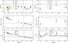 |
Fig. 5 NIR and MIR extinction toward the TMC1A jet. Same as Figure 2, but extended to include additional a4D lines in the NIR (left) used for ne derivation, along with MIR lines (right). Model scatter points correspond to the derived electron density at 10 000 K (see Section 4.2), with uncertainties reflecting the uncertainty range in the determined ne value and temperatures from 5000–10 000 K. Commonly used NIR/MIR extinction curves are overplotted for comparison (see text). |
4.3 Relative extinction between the NIR and MIR
To determine the relative extinction between the NIR and MIR, we compared the observed [Fe II] line ratios of MIR transitions (a6D, a4F at 5.3, 17.0, 24.5, and 26 µm) relative to the 1.644 µm line with the intrinsic model ratios. We first assumed that the NIR and MIR lines along the same sight lines originate from the same physical region, implying identical excitation conditions governed by the same ne and T. Next, we explore the case where MIR lines along the same sight lines trace gas described by conditions that differ from the NIR lines, with different values of ne and/or T.
The electron density derived from NIR lines (Section 4.2) serves as the reference for these comparisons at each jet location. Uncertainties in electron density and temperature contribute to the overall uncertainty range. We adopted a standard reference temperature of 10 000 K, consistent with shock models, where NIR and MIR lines become emissive at temperatures ≳7000 K (Nisini 2008; Giannini et al. 2015a; Koo et al. 2016). To account for the uncertainties, we used a lower bound of 5000 K.
4.3.1 Case 1: Same physical conditions
In the scenario where the NIR and MIR [Fe II] emission lines along the same sight lines originate from the same physical region, we first calculated the modeled line ratios, assuming the same electron density and temperature for both MIR and NIR lines, including the reference line at 1.644 µm.
Figure 5 shows the derived extinction for each line of sight toward the TMC1A j et. The left panels show NIR-derived extinction in the 1.2–1.85 µm range, including additional a4D lines not used to derive the electron density, which follows the trend observed in Section 4.1. The right panels show extinction derived from the four MIR lines observed with MIRI.
The observed MIR line fluxes are comparable to or higher than that of the 1.644 µm line (with ratios robs ~1−10), which is very different from the modeled intrinsic line ratios, which are below unity (with rmodel < l). The difference is caused by the fact that the reference NIR line at 1.644 µm experiences stronger extinction than the MIR lines, which is reflected by the negative ΔAλ shown in the middle right panel of Fig. 5.
The extinction at each jet location follows a pattern where bright regions (B, F1) exhibit higher MIR extinction than regions farther from the protostar (F2, F3), consistent with increased column density closer in. Our inferred extinction at 5.34 µm is low (βλ ~ 0), likely setting a lower limit since it is comparable to or less than the least extinct curve at that wavelength (WD1, RV = 3.1). In contrast, the extinction at 17.93, 24.52, and 25.99 µm is usually higher than the comparison curves, indicating greater attenuation at these wavelengths compared to that expected from the comparison curves.
Since robs > rmodel for the MIR lines, we find ∆Aλ < 0, and any additional suppression of the observed MIR intensity due to line blending would only make ∆Aλ less negative, thereby increasing βλ. This could be the case for the [Fe II] 17.936 µm line, which is spectrally close to the H2 υ = 1−1 S(1) line at 17.94 µm. However, as a first-order approximation, we built an H2 excitation model and interpolated the column density of H2 molecules in the upper state (υu = 1, Ju = 3) based on the energy of the corresponding upper state of H2 1-1 S(1). We then estimated the H2 1-1 S(1) line flux using the Einstein coefficient of spontaneous emission, assuming an extinction law (KP5; Pontoppidan et al. (2024)) and corresponding extinction value. This allowed us to calculate the fraction of the observed 17.936 µm line that originates from H2 and [Fe II]. We find the H2 contribution is ≪1%, confirming that [Fe II] dominates at this wavelength.
4.3.2 Case 2: Diverging physical conditions between NIR and MIR lines
The observed [Fe II] lines may originate from gas with different excitation conditions. This posits that the emitting regions are stratified, where higher excitation lines (e.g., those in the NIR) predominantly trace hotter and/or denser gas, while lower excitation lines (e.g., those in the MIR) arise from cooler and/or less dense regions along the same line of sight (within the effective telescope beam).
To explore this possibility, we consider a simplified scenario in which the NIR (∆ < 5 µm) and MIR (λ > 5 µm) lines trace two distinct temperature and density components, with
 (4)
(4)
where  and fT represent the fractional electron density and temperature of the MIR-emitting gas relative to those inferred from the NIR a4D line ratios (see Section 4.2).
For temperatures above 5000 K, the predicted line ratios converge at a given electron density, resulting in minimal temperature dependence on the derived βλ values. This is seen in the top subplot of Fig. 6, where the MIR lines are assumed to originate from gas at half the temperature of the NIR lines (fT = 0.5, TMIR = 5000 K, TNIR = 10000 K). The derived MIR βλ values are almost indistinguishable from the reference case of fT = 1 and  shown in the bottom-right panel of Fig. 5.
In contrast, electron density has a more pronounced effect on βλ. The middle subplot (fT = 1.0,  ) shows that lowering the electron density systematically reduces βλ, consistent with an increased MIR/NIR line ratio that decreases the relative difference between observed and modeled values. The bottom subplot (ƒT = 0.5,
  ) shows a similar βλ profile to the middle case, reinforcing that the electron density difference has a stronger influence on the derived extinction than temperature differences.
5 Discussion
We developed a new technique for determining the MIR extinction in the protostellar envelope using JWST IFU observations of several [Fe II] NIR and MIR emission lines, leveraging the well-determined NIR extinction curve and excitation model for line ratios. We applied this technique to the atomic jet toward the Class I protostar TMC1A, which is embedded in a large-scale infalling envelope. This technique provides a spatially resolved constraint on extinction along different sight lines to the jet, offering an independent measurement that is distinct from background star methods applied to sight lines directed away from protostars through dark clouds (e.g., McClure 2009).
This approach also complements the opacity measurements of volatile ice features in protostellar envelopes along similar sight lines, (e.g., Tyagi et al. 2025). We acknowledge that our method assumes the dust column within each beam is relatively uniform (i.e., a single AV applies) and consistent with a “screen” geometry. Figure 1 illustrates this assumption, with the top panel showing extinction measured from background stars and the bottom panel representing embedded jet sight lines that pass through a dense, infalling envelope.
When the MIR lines originate from gas in the embedded jet with physical conditions (electron density ne and temperature T) similar to those of the NIR line emitting region along the same sight lines, we will find systematically higher MIR extinction through the protostellar envelope, compared to the empirical high-extinction regime derived by McClure (2009). It also exceeds the RV=5.5 case from Weingartner & Draine (2001) and the KP5 model from Pontoppidan et al. (2024) (see the lower-right panel of Fig. 5). These models describe dust populations with larger maximum grain sizes than those in the diffuse ISM. The alignment of McClure (2009) with the RV=5.5 case has been interpreted as evidence for dust grain growth in denser cloud regions. If the MIR and NIR emission lines trace the same excitation conditions, the higher inferred extinction in the MIR toward the embedded jet suggests differences in the grain size distribution such as the presence of even larger dust grains along these sight lines. This result adds weight to the conclusion of Valdivia et al. (2019) and Le Gouellec et al. (2020) that dust grains must have grown significantly in protostellar envelopes since relatively long-wavelength local IR photons can only spin them up efficiently through radiative torques if the grains are sufficiently large, enabling magnetic alignment and the observed levels of dust polarization.
If the MIR emission lines trace lower electron density and temperature than the NIR lines, then the modeled intrinsic MIR lines would be weaker, yielding a lower inferred MIR extinction, with the resulting βλ values falling within the range predicted by background star studies (see Section 4.3.2). In this case, the extinction curve does not indicate significant changes in grain size distributions, such as dust growth beyond what is inferred along high-extinction sight lines of dense clouds. This result is still highly significant because it implies that, even along the same sight lines directed toward the embedded jet, the MIR lines must originate from gas with properties different from those of the NIR line emitting gas. This could happen if, for example, the MIR and NIR lines trace different regions behind spatially unresolved shocks in the telescope beam. Differences in excitation conditions between NIR and MIR lines (e.g., Koo et al. 2016) have been observed in the case of H2 outflows (e.g., Vleugels et al. 2025); however, to our knowledge, this has not yet been demonstrated for atomic lines from the same ionization state. If the outflow is laterally stratified, with hotter and faster moving material closer to the jet axis (as evidenced by, e.g., the nested morphology of HH 30 Pascucci et al. 2025), it is plausible for the NIR lines to trace regions closer to the jet axis than the MIR lines, but this possibility remains unproven. In any case, our result highlights the important point that it would be difficult to accurately infer the physical properties of the MIR line-emitting gas in the embedded jet unless the MIR extinction curve in the foreground protostellar envelope is adequately characterized in an independent fashion.
The method described in this paper, leveraging wide spectral coverage and integral field unit (IFU) observations, could be extended to other embedded astrophysical environments. Atomic and molecular tracers (e.g., forbidden lines, hydrogen recombination lines, and H2 with their wide spectral coverage across infrared and radio wavelengths) offer promising opportunities for applying this technique. If these tracers originate from the same spatial region and their line intensities or ratios can be reliably modeled, extinction curves could be determined. Additionally, applying this method to species tracing spatially distinct regions (e.g., spatially nested outflows) and comparing them self-consistently within the same source could provide deeper insights into the dust properties across these regions. This offers a unique perspective on the role of dynamic processes in star formation (particularly outflows) in shaping dust. Expanding this approach to more sources at different stages of star formation and along diverse lines of sight would enhance our understanding of dust evolution within protostellar environments and throughout star formation scenarios.
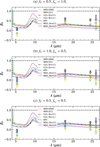 |
Fig. 6 Derived MIR extinction from [Fe II] lines (λ > 5 µm) tracing different excitation conditions compared to NIR [Fe II] lines. The plots show MIR extinction, where MIR [Fe II] lines trace different excitation conditions (ne, Te) than NIR [Fe II] lines. Top: βλ values assuming MIR line intensities correspond to gas at half the NIR-traced temperature (fT = 0.5) with the same electron density ( |


6 Conclusions
This study investigates the extinction properties and evidence of dust processing in the protostellar envelope surrounding the embedded [Fe II] jet of the Class I protostar TMC1A using JWST NIRSpec and MIRI observations and a novel technique. By combining high-sensitivity, multi-wavelength emission line data with excitation models, we derived localized extinction curves along the sight lines toward the embedded jet and compared them to extinction laws derived from dark cloud populations. These efforts aimed to understand how star formation processes influence the surrounding dust populations, contributing to differences in the line-of-sight extinction. We summarize our findings as follows:
We developed a new method for characterizing the NIR-MIR extinction of material in the protostellar envelope along the lines of sight to an embedded [FeII] jet, based on JWST NIR-spec and MIRI observations of line emissions and excitation model predictions of intrinsic line ratios.
The modeled intrinsic line ratios depend on electron density and temperature. The electron density can be reasonably well constrained by NIR [Fe II] lines (for which extinction curves are already well characterized), with values ranging from approximately 5 × 10³ to 5 × 104 cm−3, decreasing farther from the protostar, consistent with prior studies of protostellar outflows.
If the MIR lines originate from gas in the embedded jet with electron density, ne, and temperature, T, similarly to those of the NIR line emitting region along the same sight lines, we find a systematically higher MIR extinction through the protostellar envelope than those derived by McClure (2009) for dark clouds, the RV = 5.5 case modeled by Weingartner & Draine (2001), and the KP5 model from Pontoppidan et al. (2024). This result adds weight to growing evidence (e.g., from dust polarization) for significant grain growth in protostellar envelopes.
If the MIR emission lines trace lower electron density and temperature than the NIR lines, the inferred MIR extinction falls within the range of the existing values for dark clouds. In this case, there is no direct evidence for a change in the dust size distribution (i.e., grain growth) in protostellar envelopes beyond that in dense dark clouds. Instead, the observed MIR/NIR line ratios and excitation modeling suggest that the MIR and NIR lines originate from different regions along the same sightline within the embedded jet, each characterized by distinct physical conditions.
The multitude of infrared [Fe II] emission lines detectable toward protostars with JWST provide a powerful probe of both NIR and MIR extinction toward deeply embedded environments. By combining models with observations of the embedded protostellar jet toward TMC1A, we characterize dust attenuation along distinct lines of sight traced by [Fe II] emission and explore potential implications for dust properties within protostellar envelopes. Expanding this approach to a larger sample spanning different evolutionary stages and outflow inclinations will help strengthen these interpretations and will be the focus of future work.
Acknowledgements
We thank the referee for a prompt and constructive report. This work was supported in part by an ALMA SOS award, STScI grant JWST-GO-02104.002-A, NSF grant AST-2307199, NASA ATP grant 80NSSC20K0533, and the Virginia Institute of Theoretical Astronomy. This work is based on observations made with the NASA/ESA/CSA James Webb Space Telescope. The data were obtained from the Mikulski Archive for Space Telescopes at the Space Telescope Science Institute, which is operated by the Association of Universities for Research in Astronomy, Inc., under NASA contract NAS 5-03127 for JWST. These observations are associated with GO program #2104. D.H. is supported by a Center for Informatics and Computation in Astronomy (CICA) grant and grant number 110J0353I9 from the Ministry of Education of Taiwan. D.H. also acknowledges support from the National Science and Technology Council, Taiwan (Grant NSTC111-2112-M-007-014-MY3, NSTC113-2639-M-A49-002-ASP, and NSTC113-2112-M-007-027). A.C.G. acknowledges support from PRIN-MUR 2022 20228JPA3A “The path to star and planet formation in the JWST era (PATH)” funded by NextGeneration EU and by INAF-GoG 2022 "NIR-dark Accretion Outbursts in Massive Young stellar objects (NAOMY)" and Large Grant INAF 2022 “YSOs Out-flows, Disks and Accretion: towards a global framework for the evolution of planet forming systems (YODA)". D.R. acknowledges support by the European Research Council advanced grant H2020-ER-2016-ADG-743029. We also thank Sophia Spiegel for contributing to the schematic shown in Figure 1, which enhances the clarity and impact of this work.
Appendix A Supplemental material
This appendix contains supplemental tables referenced throughout the main text. Table A.1 lists atomic properties and critical densities for the [Fe II] transitions analyzed in this study.
Spectroscopic properties of [Fe II] lines observed in TMC1A.
Continuum-subtracted integrated intensities of [Fe II] lines observed at distinct jet locations.
Observed [Fe II] 1.257/1.644 intensity ratios and extinction measurements
Measured electron densities toward jet locations
References
- Argyriou, I., Glasse, A., Law, D. R., et al. 2023, A&A, 675, A111 [NASA ADS] [CrossRef] [EDP Sciences] [Google Scholar]
- Aso, Y., Ohashi, N., Saigo, K., et al. 2015, ApJ, 812, 27 [Google Scholar]
- Aso, Y., Kwon, W., Hirano, N., et al. 2021, ApJ, 920, 71 [NASA ADS] [CrossRef] [Google Scholar]
- Assani, K. D., Harsono, D., Ramsey, J. P., et al. 2024, A&A, 688, A26 [NASA ADS] [CrossRef] [EDP Sciences] [Google Scholar]
- Bjerkeli, P., van der Wiel, M. H. D., Harsono, D., Ramsey, J. P., & Jørgensen, J. K. 2016, Nature, 540, 406 [Google Scholar]
- Boogert, A. C. A., Gerakines, P. A., & Whittet, D. C. B. 2015, ARA&A, 53, 541 [Google Scholar]
- Brügger, N., Burn, R., Coleman, G. A. L., Alibert, Y., & Benz, W. 2020, A&A, 640, A21 [NASA ADS] [CrossRef] [EDP Sciences] [Google Scholar]
- Bushouse, H., Eisenhamer, J., Dencheva, N., et al. 2023, JWST Calibration Pipeline (USA: NASA) [Google Scholar]
- Bushouse, H., Eisenhamer, J., Dencheva, N., et al. 2024, JWST Calibration Pipeline (USA: NASA) [Google Scholar]
- Cacciapuoti, L., Macias, E., Gupta, A., et al. 2024, A&A, 682, A61 [NASA ADS] [CrossRef] [EDP Sciences] [Google Scholar]
- Caratti o Garatti, A., Ray, T. P., Kavanagh, P. J., et al. 2024, A&A, 691, A134 [NASA ADS] [CrossRef] [EDP Sciences] [Google Scholar]
- Cardelli, J. A., Clayton, G. C., & Mathis, J. S. 1989, ApJ 345, 245 [Google Scholar]
- Chatzikos, M., Bianchi, S., Camilloni, F., et al. 2023, Rev. Mexicana Astron. Astrofis., 59, 327 [Google Scholar]
- Christiaens, V., Gonzalez, C., Farkas, R., et al. 2023, J. Open Source Softw., 8, 4774 [NASA ADS] [CrossRef] [Google Scholar]
- Crapsi, A., van Dishoeck, E. F., Hogerheijde, M. R., Pontoppidan, K. M., & Dullemond, C. P. 2008, A&A, 486, 245 [NASA ADS] [CrossRef] [EDP Sciences] [Google Scholar]
- Dartois, E., Noble, J. A., Caselli, P., et al. 2024, Nat. Astron., 8, 359 [NASA ADS] [CrossRef] [Google Scholar]
- Decleir, M., Gordon, K. D., Andrews, J. E., et al. 2022, ApJ, 930, 15 [NASA ADS] [CrossRef] [Google Scholar]
- Decleir, M., Gordon, K. D., Misselt, K. A., et al. 2025, AJ, 169, 99 [Google Scholar]
- Delabrosse, V., Dougados, C., Cabrit, S., et al. 2024, A&A, 688, A173 [NASA ADS] [CrossRef] [EDP Sciences] [Google Scholar]
- Di Francesco, J., Johnstone, D., Kirk, H., MacKenzie, T., & Ledwosinska, E. 2008, ApJS, 175, 277 [Google Scholar]
- Drazkowska, J., Bitsch, B., Lambrechts, M., et al. 2023, ASP Conf. Ser., 534, 717 [NASA ADS] [Google Scholar]
- Erkal, J., Nisini, B., Coffey, D., et al. 2021, ApJ, 919, 23 [NASA ADS] [CrossRef] [Google Scholar]
- Ferland, G., Chatzikos, M., Guzmán, F., et al. 2017, Revista mexicana de astronomía y astrofísica, 53, 00016 [Google Scholar]
- Fitzpatrick, E. L., Massa, D., Gordon, K. D., Bohlin, R., & Clayton, G. C. 2019, ApJ, 886, 108 [Google Scholar]
- Frank, A., Ray, T. P., Cabrit, S., et al. 2014, Protostars and Planets VI (Tucson: University of Arizona Press), 451 [Google Scholar]
- Galametz, M., Maury, A. J., Valdivia, V., et al. 2019, A&A, 632, A5 [NASA ADS] [CrossRef] [EDP Sciences] [Google Scholar]
- Galli, P., Loinard, L., Bouy, H., et al. 2019, A&A, 630, A137 [NASA ADS] [CrossRef] [EDP Sciences] [Google Scholar]
- Giannini, T., Antoniucci, S., Nisini, B., Bacciotti, F., & Podio, L. 2015a, ApJ, 814, 52 [NASA ADS] [CrossRef] [Google Scholar]
- Giannini, T., Antoniucci, S., Nisini, B., et al. 2015b, ApJ, 798, 33 [Google Scholar]
- Gordon, K. D., Cartledge, S., & Clayton, G. C. 2009, ApJ, 705, 1320 [NASA ADS] [CrossRef] [Google Scholar]
- Gordon, K. D., Misselt, K. A., Bouwman, J., et al. 2021, ApJ, 916, 33 [NASA ADS] [CrossRef] [Google Scholar]
- Gordon, K. D., Clayton, G. C., Decleir, M., et al. 2023, ApJ, 950, 86 [CrossRef] [Google Scholar]
- Greenfield, P., & Miller, T. 2016, Astron. Comput., 16, 41 [NASA ADS] [Google Scholar]
- Grevesse, N., Asplund, M., Sauval, A. J., & Scott, P. 2010, Ap&SS, 328, 179 [Google Scholar]
- Harsono, D., Bjerkeli, P., van der Wiel, M. H. D., et al. 2018, Nat. Astron., 2, 646 [Google Scholar]
- Harsono, D., Bjerkeli, P., Ramsey, J. P., et al. 2023, ApJ, 951, L32 [NASA ADS] [CrossRef] [Google Scholar]
- Hollenbach, D., & McKee, C. F. 1989, ApJ, 342, 306 [Google Scholar]
- Johansen, A., Blum, J., Tanaka, H., et al. 2014, in Protostars and Planets VI, eds. H. Beuther, R. S. Klessen, C. P. Dullemond, & T. Henning (Tucson: University of Arizona Press), 547 [Google Scholar]
- Johansen, A., Ronnet, T., Bizzarro, M., et al. 2021, Sci. Adv., 7, eabc0444 [NASA ADS] [CrossRef] [Google Scholar]
- Koo, B.-C., Raymond, J. C., & Kim, H.-J. 2016, J. Korean Astron. Soc., 49, 109 [NASA ADS] [CrossRef] [Google Scholar]
- Kristensen, L. E., van Dishoeck, E. F., Bergin, E. A., et al. 2012, A&A, 542, A8 [NASA ADS] [CrossRef] [EDP Sciences] [Google Scholar]
- Law, D. R., Morrison, J. E., Argyriou, I., et al. 2023, AJ, 166, 45 [NASA ADS] [CrossRef] [Google Scholar]
- Le Gouellec, V. J. M., Hull, C. L. H., Maury, A. J., et al. 2019, ApJ, 885, 106 [NASA ADS] [CrossRef] [Google Scholar]
- Le Gouellec, V. J. M., Maury, A. J., Guillet, V., et al. 2020, A&A, 644, A11 [EDP Sciences] [Google Scholar]
- Le Gouellec, V. J. M., Greene, T. P., Hillenbrand, L. A., & Yates, Z. 2024, ApJ, 966, 91 [NASA ADS] [CrossRef] [Google Scholar]
- Le Gouellec, V. J. M., Lew, B. W. P., Greene, T. P., et al. 2025, ApJ, 985, 225 [Google Scholar]
- Mathis, J. S. 1990, ARA&A, 28, 37 [NASA ADS] [CrossRef] [Google Scholar]
- McClure, M. 2009, ApJ, 693, L81 [NASA ADS] [CrossRef] [Google Scholar]
- McClure, M. K., Rocha, W. R. M., Pontoppidan, K. M., et al. 2023, Nat. Astron., 7, 431 [NASA ADS] [CrossRef] [Google Scholar]
- Miotello, A., Testi, L., Lodato, G., et al. 2014, A&A, 567, A32 [NASA ADS] [CrossRef] [EDP Sciences] [Google Scholar]
- Narang, M., P., M., Tyagi, H., et al. 2023, Investigating Protostellar Accretion across the mass spectrum with the JWST: discovery of a collimated jet from the low luminosity protostar IRAS 16253-2429 in a quiescent accretion phase [Google Scholar]
- Nisini, B. 2008, in Jets from Young Stars II, eds. F. Bacciotti, L. Testi, & E. Whelan (Berlin: Springer), 742, 79 [Google Scholar]
- Pascucci, I., Beck, T. L., Cabrit, S., et al. 2025, Nat. Astron., 9, 81 [Google Scholar]
- Pontoppidan, K. M., Evans, N., Bergner, J., & Yang, Y.-L. 2024, Res. Notes Am. Astron. Soc., 8, 68 [Google Scholar]
- Quinet, P., Le Dourneuf, M., & Zeippen, C. J. 1996, A&AS, 120, 361 [NASA ADS] [CrossRef] [EDP Sciences] [Google Scholar]
- Sarkar, A., Ferland, G., Chatzikos, M., et al. 2021, ApJ, 907, 12 [NASA ADS] [CrossRef] [Google Scholar]
- Smyth, R., Ramsbottom, C., Keenan, F., Ferland, G., & Ballance, C. 2019, MNRAS, 483, 654 [Google Scholar]
- Sturm, J. A., McClure, M. K., Beck, T. L., et al. 2023, A&A, 679, A138 [NASA ADS] [CrossRef] [EDP Sciences] [Google Scholar]
- Tyagi, H., Manoj, P., Narang, M., et al. 2025, ApJ, 983, 110 [Google Scholar]
- Tychoniec, L., van Gelder, M. L., van Dishoeck, E. F., et al. 2024, A&A, 687, A36 [NASA ADS] [CrossRef] [EDP Sciences] [Google Scholar]
- Valdivia, V., Maury, A., Brauer, R., et al. 2019, MNRAS, 488, 4897 [NASA ADS] [CrossRef] [Google Scholar]
- van Dishoeck, E. F., Kristensen, L. E., Benz, A. O., et al. 2011, PASP, 123, 138 [NASA ADS] [CrossRef] [Google Scholar]
- Verner, E., Verner, D., Korista, K., et al. 1999, ApJS, 120, 101 [NASA ADS] [CrossRef] [Google Scholar]
- Vleugels, C., McClure, M., Sturm, A., & Vlasblom, M. 2025, A&A, 695, A145 [NASA ADS] [CrossRef] [EDP Sciences] [Google Scholar]
- Weingartner, J. C., & Draine, B. T. 2001, ApJ, 548, 296 [Google Scholar]
- Zhang, H. L., & Pradhan, A. K. 1995, A&A, 293, 953 [NASA ADS] [Google Scholar]
All Tables
Continuum-subtracted integrated intensities of [Fe II] lines observed at distinct jet locations.
All Figures
|
Fig. 1 Schematic illustrating extinction sight lines in two contexts. Top panel represents background star extinction studies through diffuse and dense regions of a molecular cloud. Bottom panel (adapted from Fig. 5 of van Dishoeck et al. 2011) shows a forming star embedded in an infalling envelope, with bipolar line-emitting jets carving outflow cavities. The JWST NIRSpec/MIRI field of view probes <1000 AU scales, with the dashed line tracing the line-of-sight path through the dense envelope, where most extinction occurs, toward the inner line emitting jet. |
| In the text | |
|
Fig. 2 [Fe II] emission lines used in this study and detected with NIRSpec and MIRI, arranged in order of increasing upper energy (EU/k). Top panels: moment-0 maps (in units of erg s−1 cm2 sr−1), constructed by integrating the emission across the frequency range indicated by the shaded regions in the corresponding spectra below. Although integration is performed in frequency space, the x-axis is displayed in velocity (km s−1) for clarity. A 3-sigma threshold is applied. The maps are overlaid with circular, color-coded apertures (0.7″) used consistently throughout this study. Bottom panels: spectra (in units of erg s−1 cm−2 sr−1 Hz−1) extracted from each aperture, with shaded regions highlighting the velocity range used for integration, primarily focusing on blue-shifted emission. Each subplot includes the rest wavelength (λ0), transition and upper energies (∆E, EU), and Einstein-A value for reference. |
| In the text | |
|
Fig. 3 NIR extinction of a4D J=7/2 lines relative to the 1.644 µm line (horizontal and vertical dashed lines.) Top: Observed (‘o’) and modeled (‘*’) line ratios for all four jet locations in this study. Middle: Difference in extinction relative to the 1.644 µm line. Bottom: Derived βλ values, normalized by the extinction at 1.644 µm, which is computed as an average over existing NIR extinction curves. This is compared with empirically determined NIR extinction curves, C89 from Cardelli et al. (1989), and the modeled extinction curves, WD1 by Weingartner & Draine (2001) and KP5 by Pontoppidan et al. (2024). We include RV = 3.1 and RV = 5.5 for applicable curves to illustrate that NIR extinction in the 1.2–1.8 µm range is largely independent of RV and shows minimal differences between independent studies. Dashed lines mark the reference line ratio, extinction difference, and βλ value at 1.644 µm (horizontal) and the wavelength of 1.644 µm (vertical) in all three panels. |
| In the text | |
|
Fig. 4 Examples of density-sensitive NIR line ratios, where the CLOUDY model predictions are shown as solid lines shaded by temperature. Observed line ratios with uncertainties are represented by circles, while extinction-corrected ratios are shown as squares color-coded by jet location (see Fig. 2). The extinction-corrected ratio, accounting for uncertainties, determines the electron density from the model, aligning with the x-axis position of both observed and corrected ratios. Top: shorter-wavelength line is more affected by extinction, leading to an increased ratio after correction. Middle: line ratio with similar rest wavelengths, minimally affected by extinction, where the observed ratio closely matches the expected electron density. Bottom: longer wavelength line that is less affected by extinction and causes the ratio to decrease after correction. Following extinction correction using established NIR curves (Section 4.1), all corrected ratios fall within the model-predicted range, showing consistent electron density trends across jet locations and line pairings. This electron density serves as a starting point for comparing relative extinction in the NIR/MIR (Section 4.3). |
| In the text | |
|
Fig. 5 NIR and MIR extinction toward the TMC1A jet. Same as Figure 2, but extended to include additional a4D lines in the NIR (left) used for ne derivation, along with MIR lines (right). Model scatter points correspond to the derived electron density at 10 000 K (see Section 4.2), with uncertainties reflecting the uncertainty range in the determined ne value and temperatures from 5000–10 000 K. Commonly used NIR/MIR extinction curves are overplotted for comparison (see text). |
| In the text | |
|
Fig. 6 Derived MIR extinction from [Fe II] lines (λ > 5 µm) tracing different excitation conditions compared to NIR [Fe II] lines. The plots show MIR extinction, where MIR [Fe II] lines trace different excitation conditions (ne, Te) than NIR [Fe II] lines. Top: βλ values assuming MIR line intensities correspond to gas at half the NIR-traced temperature (fT = 0.5) with the same electron density ( |
| In the text | |
Current usage metrics show cumulative count of Article Views (full-text article views including HTML views, PDF and ePub downloads, according to the available data) and Abstracts Views on Vision4Press platform.
Data correspond to usage on the plateform after 2015. The current usage metrics is available 48-96 hours after online publication and is updated daily on week days.
Initial download of the metrics may take a while.