| Issue |
A&A
Volume 701, September 2025
|
|
|---|---|---|
| Article Number | A200 | |
| Number of page(s) | 11 | |
| Section | Numerical methods and codes | |
| DOI | https://doi.org/10.1051/0004-6361/202555022 | |
| Published online | 16 September 2025 | |
Transmission of the AtmosPhere for AStronomical data: TAPAS upgrade
1
LIRA, Observatoire de Paris, PSL University, CNRS,
5 Place Jules Janssen,
92190
Meudon,
France
2
LATMOS, Sorbonne-Université,
Paris,
France
3
ACRI-ST,
260 Route du Pin Montard, BP234,
06904
Sophia-Antipolis,
France
4
Institut Pierre Simon Laplace (IPSL), AERIS Data Centre,
75252
Paris,
France
5
European Southern Observatory,
Alonso de Cordova 3107, Vitacura,
Santiago,
Chile
★ Corresponding author: This email address is being protected from spambots. You need JavaScript enabled to view it.
Received:
3
April
2025
Accepted:
1
August
2025
Abstract
Context. Current molecular databases and realistic global atmospheric models allow us to predict accurate atmospheric transmittance spectra. Observers with ground-based spectrographs may use this information to identify the telluric absorption lines, to correct their astronomical spectra for these lines fully or partially, or take them into account in forward models.
Aims. The TAPAS online service provides atmospheric transmittance spectra of the most important species, as well as Rayleigh extinction, adapted to any observing location, date, and direction. We describe recent updates, improvements, and additional tools.
Methods. TAPAS interpolates the location in the atmospheric profiles of temperature, pressure, H2O, O2 and O3 that are extracted from the meteorological field of the European Centre for Medium Term Weather Forecast (ECMWF) for the date and time of the observation. The composite profiles are produced by a Data Terra/AERIS/ESPRI product called Arletty, and they are supplemented by auxiliary climatological models for additional species. The transmittance spectra are computed with the code LBLRTM. The default width of the spectral pixels is chosen to ensure that the shapes of all the absorption lines are reproduced for each species. Major improvements with respect to the previous TAPAS are the extension of the wavelength range in the near-UV down to 300 nm and the extension in the near-IR up to 3500 nm; the use of the recent version of the HITRAN database (HITRAN2020); the addition of NO2 transmittance to complement H2O, O2, O3, N2O, CO2, and CH4; an increased accessibility and a reduced time to obtain the results; and the possibility to force the total H2O column to match the column measured at the observatory at the time of record.
Results. We show O3 absorption in the near-UV and near-IR and NO2 absorption in the visible. We illustrate the quality of TAPAS by means of comparisons between models and ESO/VLT/CRIRES recorded spectra of a hot star with a spectral resolution of ~130 000 in two intervals in the near-IR with strong H2O, N2O, CO2, and CH4 absorption. We describe the measurement of an instrumental line spread function based on TAPAS O2 lines and a method using the singular value decomposition technique that can be made entirely automated.
Conclusions. The new TAPAS tool provides realistic simulations of the telluric lines. It gives access to the weakest H2O or O2 lines, and to the very weak highly irregular NO2 lines. It can be used to improve the wavelength assignment when calibration lamps provide only a few emission lines, and to accurately measure the line spread function in most regions in which telluric features are present. The extended wavelength range will be particularly useful for future or recent spectrographs in the near-UV and in the near-IR.
Key words: line: identification / atmospheric effects / instrumentation: spectrographs / techniques: spectroscopic
© The Authors 2025
 Open Access article, published by EDP Sciences, under the terms of the Creative Commons Attribution License (https://creativecommons.org/licenses/by/4.0), which permits unrestricted use, distribution, and reproduction in any medium, provided the original work is properly cited.
This article is published in open access under the Subscribe to Open model. This email address is being protected from spambots. You need JavaScript enabled to view it. to support open access publication.
1 Introduction
Telluric absorption is a contaminant of astronomical spectra that must be taken into account and, ideally, eliminated from the data. As a result of the tremendous improvements made over the past few decades in the meteorological fields on the one hand and for molecular data on the other hand, it has become possible to perform this correction based on a predicted model of the telluric transmittance spectrum (see Lallement et al. 1993, for a first application with the GEISA spectroscopic database). This replaces the division by the spectrum of a smooth continuum comparison star that is recorded under the same conditions as those of the target of interest. This procedure saves observing time and avoids features in the spectrum of the comparison star. To this end, the free service TAPAS was launched in 2012 and has been online since 2014 (see Bertaux et al. 2014, for details). During the past decades, telluric corrections became more frequent, were sometimes routinely done, and new wavelength ranges that are contaminated by telluric features could be used. Observations that require especially accurate telluric corrections are those dedicated to exoplanets. In the case of radial velocity measurements, residuals of insufficiently corrected telluric lines or undetected so-called micro-tellurics perturb the periodic signals from planets. In the case of transit spectroscopy, which aims to detect an atmosphere around an exoplanet and to identify the presence of gases such as CO2 and H2O, the correction is of crucial importance. The tiny circular atmosphere around the exoplanet gives a spectral signature, as a tiny change in the spectrum of the host star, and very precise measurements of the much stronger variations in the telluric features are mandatory.
TAPAS1 (for Transmission of the ATmosphere for AStronomical data) simulates the atmospheric transmission spectra from the main absorbing species with exquisite detail as a function of date, observing site, and either zenith angle or target celestial coordinates. TAPAS uses the Arletty facility from the Ensemble de Services pour la Recherche à l’IPSL (ESPRI) Data and Services Centre from the Institut Pierre-Simon Laplace (IPSL), which is part of the Data Terra/AERIS (a French Atmospheric Chemistry Data Centre) infrastructure. Arletty (Hauchecorne 1999) computes vertical pressure, temperature, and H2O, O2, and O3 profiles extracted from the extremely detailed model of the global atmosphere produced by the European Centre for Medium-Range Weather Forecasts (ECMWF) using a grid of 0.5 degree in longitude and latitude. The ECMWF profiles are refreshed every 6 hours through assimilation of new data from the space and from the ground. Arletty selects the model closest in time to the observer’s request and interpolates it in location within the ECMWF grid. Additional models based on the data are used to calculate the distributions of N2O, CO2, and CH4. For each date, TAPAS interpolates the measurements of the annual evolution of the mean abundance of these species to select the appropriate value of the relative abundance to dry air (or mixing ratio), and it then distributes the concentration of the species in altitude following this fixed mixing ratio and the pressure and temperature altitude profiles.
Atmospheric transmittance spectra are integrated from the altitude of 70 km to the altitude of the observatory in each of the altitude layers of ECMWF, and above 70 km in the climate model MSIS-90. They are based on molecular data from the HITRAN database (Rothman 2021; Gordon et al. 2017; Gordon et al. 2022) and are computed by means of the line-by-line radiative transfer model (LBLRTM) (Clough & Iacono 1995; Clough et al. 2005). For each species and each altitude layer, the local temperature and pressure are used to compute air- and self-broadening as well as the pressure line shift for each HITRAN transition. TAPAS calculates the transmittance separately for each isotope present in HITRAN using standard terrestrial abundance ratios. For the basic mode of the TAPAS output, the grid spacing is automatically chosen to be small enough to accurately represent each atmospheric line from each species. The resulting grid steps are on the order of 1 mÅ (resolving power R ≃ 5 × 10⁶ at 1000 nm, assuming a resolving power element is sampled by two grid steps). This is important because it opens the possibility to reproduce their exact shapes and determine the instrumental function of the spectrographs (see Section 3). The transmission spectra may be obtained separately for individual gases. The spectra can be transformed in the observer’s frame or in the Solar System barycentric frame, and they can be convolved to be adapted to any spectral resolution.
The telluric features in the user-recorded spectra are not removed by TAPAS itself, which is different from the ESO software MolecFit Smette et al. (2015), for instance, or from the tool Telfit (Gullikson et al. 2014). Instead, it provides the necessary detailed information to perform a correction, without the need to install a local software. The main difference between TAPAS and the above mentioned tools for transmittance spectra is the choice of the global atmospheric model, the European ECMWF for TAPAS, and the US global data assimilation system (GDAS) model for the two other tools. TAPAS serves as a basis for the line identifications or for various post-processing correction techniques. The best transmittance models are obtained easily, rapidly, and online species by species, to be subsequently used by the user in various ways. This allows the user to identify which feature is of telluric origin, to predict the telluric contamination of planned observations, and to use the transmittance spectra in locally developed codes of telluric removal or in forward models that combine telluric and astronomical information.
Several simple or sophisticated techniques have already been implemented by different groups to use modeled atmospheric transmittance spectra to correct astronomical spectra for telluric contamination. The simplest techniques adjust the model to the data by varying the instrumental function of the spectrograph, the wavelength offset between the data and the model, if necessary, and the absorber columns Ai (i=1,N for N different absorbers). This latter adjustment makes use of N free parameters Xi and TXi(Ai), which is the model transmission T(Ai) raised to the power Xi, corresponding to an increase in the column of the absorber Ai by a factor Xi. In practice, TAPAS predicts very accurate transmissions for all species except H2O, and in this case, N=1 (see Section 2). Because the integrated water vapor varies on timescales of hours or even minutes, the water vapor transmittance cannot be predicted accurately. Local measurements based on a radiometer (Smette et al. 2020) can be used, but at the time of writing, the retrieval algorithms used by the radiometers at Paranal tend to underestimate the amount of precipitable water vapor for values below ≃1 mm (see also Ivanova et al. 2023). For weak to moderate absorption, a very simple way to determine a value of Xi that fits the data best and to adjust the instrumental function and the wavelength offset is to use the minimization of the length of the spectrum that was obtained after division of the data by the model as a criterion. This rope-length method uses the fact that for the optimal model, there are no irregular residuals whose effect is a significant increase in the length of the spectrum (e.g. Cox et al. 2017; Cami et al. 2018; Elyajouri et al. 2018). For stronger lines, another method is to adjust the data to a forward model based on the product of the telluric transmittance by another function, which can be a continuum (e.g. Ivanova et al. 2023), the product of a continuum and an absorption band (e.g. Puspitarini et al. 2013), the product of a continuum, a modeled stellar spectrum and an absorption band (e.g. Puspitarini et al. 2015), or other functions. This forward-modeling technique is necessary in the case of cool stars, whose spectra contain numerous deep and narrow lines. Intermediate methods using both rope-length minimization and forward modeling have also been proposed (Cami et al. 2018). Finally, sophisticated adjustments by means of the chi-square method were used by Molecfit Smette et al. (2015). They include the possibility to vary the shape of the instrumental function in addition to the wavelength offset, spectral resolution, and abundances. In the case of very strong lines, in particular, in the red or near-IR domain, the correction for telluric lines becomes extremely sensitive to very small discrepancies between the model and the data. The downloaded transmittance can be modified to remove the residuals that arise from these small discrepancies. This is the case, for example, of the APERO technique developed by Cook et al. (2022) and used for CFHT/SPIROU observations. APERO uses the residuals extracted from the spectra of hot stars that were initially corrected based on TAPAS transmittance spectra to produce a correction database (e.g. Artigau et al. 2014, 2021) and perform a refined PCA-based correction.
The TAPAS facility has recently been updated, and the purpose of this document is to illustrate this evolution. The main type of improvement concerns the computations of the transmittance spectra. It includes an important extension of the wavelength range in the near-UV from 350 nm to 300 nm, and in the near-IR from 2500 nm up to 3500 nm. This may be useful in the context of developing a new generation of spectrographs in these ranges, namely the Cassegrain U-Band Efficient Spectrograph (CUBES) at ESO/VLT (Cristiani et al. 2022) in the near-UV, and CRIRES at the ESO/VLT (Dorn et al. 2023) in the near-IR. Updates were made of the models that are used to calculate the distributions of N2O, CO2, and CH4. For dates before 2002, the data were extracted from the World Data Centre for Greenhouse Gases2 and the Global Monitoring Laboratory3. For dates since 2002 and later, TAPAS uses the most recent values from the Copernicus Atmosphere Monitoring Service (CAMS)4. Updates also include the addition of the NO2 transmittance to complement H2O, O2, O3, N2O, CO2, and CH4. Moreover, the user can force the H2O model to the humidity conditions measured at the observatory at the time of record. This may be useful for instruments that reach the near-IR domain, such as SPIRou at the Canada France Hawaii Telescope (Donati et al. 2020), GIANO at the TNG telescope (Origlia et al. 2014), CARMENES at the Calar Alto Observatory (Quirrenbach et al. 2012), and the NIRPS at the ESO/La Silla 3.6-meter telescope (Wildi et al. 2017). Last but not least, another improvement is the use of the most recent version of the HITRAN database (HITRAN2020). On the other hand, the TAPAS interface has also been substantially improved. It contains additional explanations to facilitate the user choices and additional information as part of the downloaded spectra. It allows several formats for the retrieved models, and the parameters can be saved for series of similar requests. Finally, a last type of update concerns the atmospheric model. TAPAS benefits from the constant improvements of the ECMWF model. One of its main changes is the increase in the number of altitude layers from 70 to 137. The expected differences, for the telluric transmittance spectra for ground-based observations in this case, are very small, because the altitude coverage was already very good at low altitudes where most of the absorption lines are built. Still, it can only improve the line shapes.
In Section 2, we show transmittance spectra in the new wavelength intervals. For the near-IR domain, we compare the TAPAS predictions with high-quality spectra with a high signal-to-noise ratio of a hot star recorded with the CRyogenic InfraRed Echelle Spectrograph (CRIRES) at the ESO/VLT (Dorn et al. 2023). In Section 3, we show how TAPAS transmittance spectra can be used to determine the instrumental line spread function (LSF) of a spectrograph. We used the technique based on the singular value decomposition (SVD) of the matrix linking the LSF to the data. We describe the online facility in Section 4.
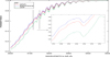 |
Fig. 1 Example of transmittance spectrum of O3 in the near-UV. A zoom into one of the intervals is inserted to show some of the very small details. |
2 New transmittance spectra
2.1 O3 absorption in the near-UV and near-IR
The extension of the TAPAS domain opens new perspectives. The addition of the 300–350 nm interval allows us to obtain very precise transmittance spectra of O3, which is a strong absorber in this area. These models can easily be obtained for any period of time and observation conditions, and they may be useful for simulating data from the future VLT/CUBES spectrograph of ESO, for instance. We show in Fig. 1 the absorption by O3 as an example for ESO Paranal in May at zenith. The absorption pattern is very complex and includes features of very different spectral widths, as illustrated in the zoomed interval. In the nearIR, the addition of the 2500 to 3500 nm interval allows us to simulate data from spectrographs such as CRIRES. We show in Fig. 2 the O3 absorption bands between 3000 and 3400 nm for ESO Paranal in May for an airmass of 2.
2.2 H2O, N2O, CO2, and CH4 in the near-IR
We illustrate the quality of the tool with two examples of comparisons between TAPAS predictions and recorded CRIRES spectra of the hot star β CMa in two different spectral intervals in the L band (2862 to 2897 nm and 3346 to 3406 nm, respectively). The setting we used was L3377 with a slit width of 0.2″. Figs. 3 and 4 show predicted transmittance spectra appropriate to Paranal, the observation date, and the direction of the star for H2O, N2O, and CO2 and H2O, CH4, and O3 respectively. The water vapor column measured at the observatory and indicated along with the data was imposed, and it was subsequently refined by elevating the transmittance at an adjusted power. For the exceptional condition of low humidity and a radiometer-predicted column of 0.51 mm at the zenith, we had to raise the TAPAS output H2O transmittance to a power 1.3 (i.e., we increased the column by 30%). Other species were kept unchanged. The products of the transmittance spectra for the relevant absorbing species were convolved with a Gaussian instrumental function, and the data were fit to the product of this resulting spectrum by a fifth-order polynomial function that represented the stellar spectrum as seen by the spectrograph. The coefficients were let free to vary. Prior to this adjustment, the offset in wavelength between the model and the data was computed for all spectral bands based on the telluric features, and we assumed that they provide the optimal calibration. The introduction of this offset was made necessary by the lack of features in the spectra of the calibration lamps in these CRIRES spectral regions and the resulting uncertain wavelength assignment. To do this, single-value offsets were first determined in consecutive intervals of 500 pixels, and the resulting series of measured offsets was subsequently fit to a second-order polynomial function of the pixel number, as illustrated in Fig. 5 for the wavelength interval of Fig. 4. This function represents the wavelength difference between the value issued from the calibration and the value issued from the telluric features and was subsequently imposed in the final adjustment of the data model.
Because only telluric features shape the spectrum of this target star, which is characterized by a smooth continuum, it was possible to appreciate the excellent quality of the predictions (see Figs. 3 and 4). A careful inspection of the correspondence between data and the TAPAS model revealed only a few very weak and narrow features in the second interval that were absent in the model. These lines are due to C2H6. C2H6 and HCN produce a few very weak absorptions in the 3000–3500 nm domain and will be the subject of future work. During the continuum-adjustment process, we initially imposed a fixed resolving power R of 90 000, but this value appeared to be significantly too low. In order to obtain a good fit, we had to increase R up to 130 000. This is linked to the use of adaptive optics (see below).
There are some important aspects of the use of models such as TAPAS for instruments such as CRIRES. In this spectral domain, very few emission lines from calibration lamps can be used, which results in a poor wavelength calibration. Because the number of telluric features is very large in this spectral domain and because telluric lines are distributed throughout all spectral intervals we considered, we were able to use the TAPAS transmittance spectra to derive a precise wavelength calibration for all the intervals, with uncertainties lower than 2 mÅ (see Fig. 5). A second aspect is linked to the spectral resolution. Adaptive optics is so efficient that the image of the target may be smaller than the entrance slit of the spectrograph (see Dorn et al. 2023). This results in a very high resolution, which is very positive, but precludes the prediction of the resolving power as a function of the slit width. Many of the telluric features are so narrow that they can be efficiently used to adjust the actual spectral resolution. For the β CMa spectra shown in Figs. 3 and 4, the resolving power was found to be on the order of 130 000, for example, which is significantly higher than the resolution that can be achieved for a target that fills a slit width of 0.23″. Finally, again because the telluric lines are distributed over many spectral intervals, the variation in the resolving power can be determined along an echelle grating order.
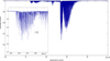 |
Fig. 2 Example of a transmittance spectrum of O3 in the near-IR domain. A zoom into one of the strongly absorbed spectral regions is inserted. |
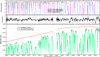 |
Fig. 3 Example of the comparison between TAPAS predictions and a CRIRES spectrum of the hot star β CMa. Top: three transmittance spectra of H2O, N2O, and CO2 computed by TAPAS and before convolution are shown (right scale). Bottom: Data (in black) fit to the product of their convolved product by a fifth-order polynomial (green curve). The fit polynomial is displayed separately (red curve). The central gap in the data is due to the transition between the second and third detector of the instrument. Middle: differences between the data and the model expressed as the percentage of the fit continuum. The two broad and shallow features marked by S cannot be residual telluric features and are very likely stellar. |
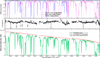 |
Fig. 4 Same as Fig. 3 for a different spectral interval characterized by absorption lines of H2O, CH4, and O3. Top: TAPAS transmittance spectra (right scale). Bottom: data (in black) fit to the product of their convolved product by a fifth-order polynomial (green curve). The fit polynomial is displayed separately (red curve). The two data gaps are due to the transitions between the detectors of the instrument. Middle: differences between the data and the model expressed as the percentage of the fit continuum. A few weak and sharp absorption lines are absent from the model and were identified as due to C2H6 and HCl (see text). |
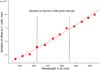 |
Fig. 5 Evolution of the difference between initially assigned wavelengths and refined telluric-based wavelengths for the data from Fig. 4 in intervals of 500 pixels. The average wavelength offset was removed. The vertical black lines show the locations of the gaps between the detectors. The red line shows the polynomial we used in the model shown in Fig. 4. |
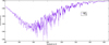 |
Fig. 6 Example of a transmittance spectrum of NO2 for ESO-Paranal in May and for an airmass of 2. The absorption depths are very small, but the irregular pattern makes this absorbing species difficult to identify. |
2.3 NO2 transmittance
NO2 is a newly added species. Its quantity is obtained from the NO2 climatology calculated by the REPROBUS 3D chemical-transport model (Lefèvre et al. 1994). The latest version has been described by Diouf et al. (2024). The amount of NO2 that is considered in TAPAS varies with the latitude and month. NO2 produces very weak lines, always weaker than one percent of the continuum in normal conditions. Its absorption features extend from 300 to 700 nm in a widely used spectral region, however, especially for extrasolar planet studies. It may be a contaminant in the case of data with a very high signal to noise ratio (S/N) and when ultraweak signals are searched for. We show in Fig. 6 the NO2 absorption for ESO-Paranal in May as an example for an airmass of 2. Its very irregular series of features are characterized by a wide range of width and shape. They are hard to identify without a full model.
2.4 HITRAN 2016 to HITRAN 2020
The update of the HITRAN version from HITRAN 2016 (Gordon et al. 2017) to HITRAN 2020 (Gordon et al. 2022) brings additional improvements. It is expected that the new version includes new weak lines and corrects for small wavelength shifts in already present lines. It is beyond the scope of this article to review all differences between the two versions. Instead, we illustrate two changes in Fig. 7. Based on ESO VLT/ESPRESSO spectra, Allart et al. (2022) described a few cases of discrepancies between the modeled and observed positions of the H2O lines that were detected in the P-Cygni type profiles that were obtained after the data were divided by the model. The modeled line was found to be slightly redshifted (blueshifted) with respect to the data for the first (second) case. We compared the new and previous versions of HITRAN for the same dates and directions for the two most discrepant cases observed by the authors. The results are displayed in the figure and show that the two main lines are displaced in a way that diminishes the discrepancy, that is, blueshifted (redshifted). These corrections may be very important, in particular, for radial velocity measurements. Additionally, we note a new weak line in the red part of the spectral interval in the second plot that was not present in the HITRAN 2016 version. We caution that these changes may not be the most important ones, and that the changes are not restricted to H2O.
3 Using transmittance spectra to retrieve the LSF
Transmittance spectra provided by the TAPAS facility can be obtained with or without convolution by the LSF representing the instrumental broadening. In the latter case, the available spectral steps (e.g., ~1.0 × 10⁻³ Å at 5000 Å) are much narrower than the widths of the telluric lines, and all spectral features of the model are reproduced in their integrality without any broadening, or with a so-called pseudo-infinite resolution. Therefore, these spectra can be used together with the observed data to derive the spectral LSF of the spectrograph. In the case of an echelle spectrograph, when H2O or O2 lines are distributed over one echelle grating order, the evolution of the LSF can be derived along the order, and the spectral analyses can be refined. This is particularly easy to do when the target spectrum is relatively smooth. A dedicated short exposure of a hot bright star is perfectly adapted to this exercise. We illustrate the use of the telluric O2 B band in spectra of two bright stars observed with the ESO ESPRESSO spectrograph (Pepe et al. 2021) and the adapted TAPAS O2 transmittance to derive the spectrograph LSF. We used the method developed by Rucinski (1999) based on the singular value decomposition (SVD) of the matrix that contains the model and links the LSF to the data. The SVD technique was already used by Seifahrt et al. (2010) for CRIRES data. We describe a new method for selecting the optimal number of singular values (SVs) below.
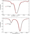 |
Fig. 7 Examples of changes from HITRAN 2016 to HITRAN2020. We use two of the small discrepancies between data and model detected by Allart et al. (2022) for the H2O lines, based on ESPRESSO spectra. The P-Cygni profiles found by the authors indicate that the deep part of the modeled line at 7184.6 Å was slightly blueshifted with respect to the data (see the double structure at the bottom in the top plot, which results in a global blueshift), while it was the opposite in the spectral regions shown in the bottom panel. The new HITRAN prediction shifts the lines in a way to correct for these effects. We also note the new weak line that is predicted by HITRAN 2020 at 7235 Å and was absent in HITRAN 2016. |
3.1 Preparation of the data and model
The LSF retrieval by means of Rucinski’s method requires the normalization of the data and the model in the spectral region that is used. This can be done for the data by masking the telluric lines, fitting the spectrum to a polynomial in unmasked regions, and dividing the spectrum by the adjusted polynomial function. The situation is different for H2O lines and O2 bands for the model. The model for the H2O lines is already normalized everywhere, and no modification is required. The collision-induced absorption (CIA) for the O2 bands generates a weak absorption in the continuum between the lines that results in a transmittance slightly below one. In this case, the same adjustment as for the data has to be performed. The second condition is that the equivalent widths (EWs) of the observed and modeled absorption features must be identical. To do this, it is sufficient to raise the normalized transmittance spectrum to the power X, where X is the ratio of the equivalent width of the lines in the data and the equivalent width of the corresponding lines in the model.
We first chose the ESPRESSO spectrum of the B0 Ib star HD 164402 as the data. The star was observed in the ultrahigh resolution mode R ~ 190 000. The spectral region was a fraction of the O2 B band that included eight strong lines in a region devoid of H2O lines. Figure 8 shows data and the TAPAS model after their normalization and after the adjustment of the EWs in this spectral interval. We downloaded this O2 model for the following parameters: Observing site= ESO Paranal; date for the atmospheric model: 2019-03-17 at 09H33 TU; no choice of any spectral resolution (to obtain the actual unconvolved transmittance); O2 lines alone; no Rayleigh extinction. The target was observed at an airmass very close to one, and we therefore selected a null zenith angle. It is also possible to enter the target coordinates when the zenith angle corresponding to the observations is unknown. The data are kept in the barycentric frame, and the required TAPAS is geocentric. Neither data nor model need to be adapted to a unique reference frame. The Doppler shift between the telluric features in data and their corresponding features in the model are accounted for in the computation of the LSF.
3.2 Algorithm
We briefly describe the principle of the LSF retrieval. Details of the technique and of its advantages over other methods can be found in Rucinski (1999). Mathematically, the problem is to find a solution to an overdetermined linear system of n equations and m unknowns with n>m,
![Mathematical equation: $\[\mathbf{Y}=\mathbf{D}.\mathbf{X},\]$](/articles/aa/full_html/2025/09/aa55022-25/aa55022-25-eq1.png) (1)
(1)
where X is a column vector containing the LSF profile on a discretized grid with m points, and Y is a column vector containing the observed spectrum on n points. D is the so-called design matrix, where the n lines are constituted by a series of m points of the TAPAS spectrum, shifted by some values at each successive line, according to the wavelength values of the Y vector. The technique proposed by Rucinski (1999) is a solution of these linear equations using the singular value decomposition (SVD) (Press et al. 1986). It consists of decomposing the design matrix D into the product of three matrices, D = U.W.VT, where U and V have orthonormal columns, VT is the transposed V, and W is a square diagonal matrix containing m SVs wi by decreasing order of magnitude. It implies the computation of the inverse matrix W−1, which is also a diagonal matrix containing the inverse 1/wi of the SVs. The trick is to keep only a limited number k of the highest SVs of the matrix W, to replace the highest last m-k values 1/wi of W−1 by zero, and to then proceed to invert the system, as described below in more detail. The solution is given by X = VW−1(UT Y). When too many SVs are kept, the noise in the data begins to be fit, which results in physically unrealistic wiggles in the LSF.
We coded this algorithm and used it to determine the LSF based on the ESPRESSO data and TAPAS models described above. In addition to the data and model, the method requires the choice of two parameters, the wavelength interval over which the LSF must be calculated, which must be wide enough to include at least one strong feature, and the number of points (which must be odd) that is used to define the LSF itself, which must be large enough in such a way that the corresponding wavelength step is significantly smaller than the expected LSF width. We used 101 points distributed over 0.25 Å.
Fig. 9 displays the SVs of the diagonal matrix computed for the data and model of Fig. 8. The first value is close to unity and is not shown. The values decrease by five orders of magnitude between solution orders 1 and 100 (and by seven orders of magnitude from order zero). A change in the shape is visible at about order 30, which is confirmed by the departure from a second-order polynomial fit performed between orders 1 and 17 and extrapolated beyond. The meaning of this change is that not meaningful SV values appear that correspond to noise fitting. In Rucinski’s presentation, the author used a very high-resolution spectrum of the same object instead of a computed model such as TAPAS to find the LSF of a lower-resolution spectrum. In this case, the noise SVs correspond to actual noise in the flux of the high-resolution spectrum that was used as a model, and the change in the shape is spectacular. Here, the TAPAS model does not have any actual flux noise and only extremely low numerical noise. The evolution of the SV along the diagonal is therefore much less spectacular than for the actual noise in the data.
Fig. 10 displays the evolution of the computed LSF profile when the solution order increases (from bottom to top). It shows the change when SVs above around 30 are taken into account more clearly. The profiles become entirely unrealistic, with an oscillatory aspect and strong negative values. The valid range between about 10 and 30 is also made particularly clear, and an almost constant profile is marked by a well-defined peak. The peak is not centered, which reflects the Doppler shift between the data and the model. Profiles corresponding to solution order 17 and 25 (whose locations are marked) are displayed and compared in Fig. 11. The order 17 profile corresponds to almost flat values outside the LSF peak area, while order 25 starts to show an oscillatory behavior. These oscillations affect the width of the LSF, which means that the width is more uncertain. At variance with order 25, the central region for order 17 is independent of any oscillation and corresponds to the actual LSF. The optimal solution is easily determined by computing the length of the profile and choosing the order corresponding to the minimum length in the good area, as illustrated in Fig. 12. This corresponds to the secondary minimum, because the primary minimum was reached at the first SV. Profiles with oscillations will have a longer length and will be discarded. This criterion is more robust than selecting the minimum width of the peak area, which is determined, for example, by fitting a Gaussian to the LSF. This is more strongly perturbed by the oscillations, as mentioned above, which may slightly and spuriously decrease the width. According to the length criterion, the solution order 17 is the optimal solution.
We show in Fig. 13 the TAPAS transmittance after convolution by the order 17 profile for the whole spectral interval and superimpose it on the data. The data and the model are indistinguishable. The difference between the data and the model is shown in the top panel. There are no particular features at the locations of the oxygen lines, which shows the quality of the LSF adjustment. For one of the lines that are shown separately, the transmittance convolved by the order 25 profile is superimposed. It is similar, and only extremely small oscillations appear on the blue side. A convolution with a Gaussian fit to the order 17 profile (not shown) does not differ significantly from a convolution using the SVD-derived profile. Both can be used for the data analysis. The selection of the order corresponding to the second LSF minimum length (here, order 17), as illustrated in Fig. 12, has the advantage of providing an automated criterion, however, and it is more accurate because as Figure 11 shows, the computed LSF is slightly different from a Gaussian. This agrees with the results of Schmidt & Bouchy (2024).
Figures 11 and 12 also display the optimal profile and the corresponding criterion for the high-resolution (HR) ESPRESSO spectrum of the early-type star HD 40111. For this spectrum, the secondary minimum of the profile length corresponds to 15 SVs. The LSF was found to be much wider than for the UHR spectrum, as expected. When the 17 SVs profile found for HD 164402 was fit with a Gaussian, the corresponding resolution was R (UHR) ≃ 225 000. This is somewhat above the value deduced from the top part of Fig. 11 by Pepe et al. (2021) for order 130 and pixel 3300 (for a wavelength of ≃6300 Å), which is about 210 000. The authors cautioned in a note, however, that their determinations of R for the UHR spectra may correspond to a lower limit. A better comparison can be obtained for the HR mode and the HD 40111 spectrum. In this case, the resolution deduced from the 15 SVs profile is R(HR)=143 000. According to the digitization of the middle part of Fig. 11 in Pepe et al. (2021), whose results for order 130 are displayed in Fig. 8 in Ivanova et al. (2023), the expected resolution around pixel 3300 is R ≃ 148 000, which is quite close to our determination.
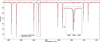 |
Fig. 8 Retrieval of the LSF. A fraction of an ESPRESSO spectrum of the hot star HD 164402 is superposed (in red) in the barycentric frame, and the downloaded atmospheric O2 transmittance spectrum adapted to the observing conditions is overplotted as well (in black). A zoom into one of the O2 line is inserted. The data were kept in the barycentric frame, as issued from the pipeline, while the TAPAS transmittance is in the geocentric frame. This explains the Doppler shift between the two. This Doppler shift is accounted for in the computation of the LSF. |
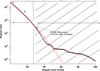 |
Fig. 9 SVs of the diagonal matrix. The first value is omitted. A second-order polynomial fit to the region delimited by points A and B is shown in red. The SVs start to depart from this function at an SV number of about 30. Beyond this region, SVs are very low and correspond to numerical noise fitting (see text). |
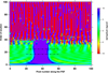 |
Fig. 10 Evolution of the LSF profile with the order of solution. Low values (at the bottom) do not reveal any acceptable shape and must be discarded. Above an order of about 30, profiles become unrealistic with the appearance of negative values. They correspond to noise fitting. In between, there is some stability around a well-defined profile. |
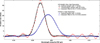 |
Fig. 11 Instrumental function profile (black curve and markers) for the ESPRESSO UHR spectrum of HD 164402 and 17 SVs (corresponding to the bottom dot-dashed black line in Fig. 10), and the associated Gaussian fit. We show the profile computed for 25 SVs superposed (red dots). An oscillatory pattern is clearly visible, suggesting that this number of SVs is already too large. Also displayed are the 15 SVs optimal profile for the ESPRESSO HR spectrum of HD 40111 and its corresponding Gaussian fit. |
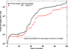 |
Fig. 12 Illustration of the criterion for the optimal number of SVs. The secondary minimum of the profile length corresponds to 17 SVs for HD 164402 (black curve) and 15 SVs for HD 40111 (red curve), their respective optimal solutions. |
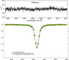 |
Fig. 13 Top: differences between the HD 164402 ultrahigh-resolution data and the TAPAS model after its convolution by the profile of the 17 SVs solution. The comparison with Figure 8 shows that there are no marked residuals at the locations of the telluric lines. Bottom: zoom into one of the lines in the UHR spectrum. In addition to the model convolved by the 17 SVs profile (green curve and dots), the result of the convolution by the 30 SVs profile is represented (red curve and plus signs). The two solutions are similar, but the former results in a slightly more regular continuum, demonstrating its superiority. |
4 Using TAPAS
The advantage of TAPAS is its ease of use. We detail all the steps below. After reading the TAPAS presentation on the home page5, users first need to select the request form menu, indicate an email address, and choose a password. An e-mail will be sent to the indicated address, and after verification of the address, the service will be available immediately. For each request, use the request form.
All items from the request form page must be filled out. For each item, a question mark provides information on the way to fill out the required parameter. We advise users to consult this detailed information for the first use of TAPAS. First, a list of the main astronomical observatories is proposed. If observing from a location that is not listed, users may enter the longitude, latitude, and altitude of the observing site. Users may suggest the addition of an observatory. Second, a date must be entered and the UT time of the observation. Third, a spectral unit for the transmittance must be chosen. Three choices are proposed: nanometers in vacuum, nanometers in standard air conditions, or a wave number in cm−1.
TAPAS proposes direct line-by-line calculations or a convolved transmittance. The former case is useful when an instrumental function is to be measured or adjusted, as detailed in Sections 2 and 3 and/or when the recorded spectra have a very high resolution. The second option allows users to obtain a transmittance adapted to any chosen spectral resolving power, based on a Gaussian instrumental function. For this second option, a sampling ratio must be indicated. It allows the user to adapt the wavelength (or frequency) step of the model to the actual pixel size of the observation and to reduce the length of the downloaded file. Then a spectral range must be entered.
In addition to observing location and date, users are offered two choices, namely a zenithal angle, or the equatorial coordinates of the target. The target coordinates are necessary when a transmittance in the barycentric frame is desired (see below). The following step is the choice of atmosphere model. For recorded data, users are advised to use Arletty, the atmosphere interpolated in the ECMWF model. In this case, the TAPAS request should be sent at least two or three days after the observing date. In other cases, estimates of atmospheric transmittance in average conditions, namely six atmospheric standard models, are proposed.
The case of water vapor is particular. Humidity conditions vary rapidly, on timescales of hours or even minutes, and ECMWF computations may not follow these rapid variations. If the observatory provides a measurement of the water vapor vertical column (usually determined by means of a radiometer) at the time of the observations, the user is advised to enter this value in the request form. In this case, TAPAS will keep the shape of the vertical profile computed by ECMWF, but scale the water vapor densities to match the on-site measurement. We tested this tool and found that it provides the water vapor lines quite close to the observed ones. When exposures are long and especially for low water vapor pressure, the amount of water vapor deduced from the radiometer may not perfectly correspond to the actual value because radiometer measurements do not perfectly predict atmospheric columns (see, e.g. Ivanova et al. 2023). This apparently applies in particular to situations of extremely low water vapor, as we found in Section 2 for CRIRES data. One way to solve this problem is to download the water vapor transmittance independently of the other species (see below), and to modify the transmittance during a post-processing by elevating it to the power of a free coefficient α until the H2O modeled lines coincide with the data. Because there are so many water vapor lines, the coefficient α is easy to determine.
The output parameters of TAPAS products are selected in the second column of the request form page. Several formats are proposed, including FITS, VO, ASCII, and NetCDF. The transmittance spectra can be obtained in the observing location frame (do not select BERV from the menu in this case) or in the barycentric frame (select BERV) to allow a direct comparison with pipeline products using this frame. The various contributions to the transmittance, that is, the Rayleigh extinction and the absorption by the proposed seven species, must then be selected. Unless the detailed shape of the spectrum is of interest, the Rayleigh extinction can often be skipped because it is very smooth and can be considered to be part of the continuum. Finally, the last choice is important: The transmittance spectra can be obtained separately or in a unique file after merging. The user is advised to select the former case, which offers the possibility of adjusting the quantity of water vapor independently of the other species.
Frequently, users need data for series of dates or series of spectral intervals for the same observatory. TAPAS allows duplicating all the parameters of a request (use the ADD menu item) and modifying one or more parameters in the added request. All the requests are executed as part of a unique submission, and all results are stored in the same directory. The number of combined requests is not limited if the execution time for the full series of requests is compatible with the system. This condition is most often achieved.
5 Conclusions and perspectives
TAPAS offers atmospheric transmittance spectra that are fully adapted to an observing site, a date, and either a zenithal angle or target coordinates online and in a very short time. We have described the improvements of the TAPAS tool, which mainly are a wavelength range evolution to reach 300 to 3500 nm, and the use of HITRAN 2020. The main advantage of TAPAS is that it is very easy to use and convenient for observers who wish to identify spectral features, to predict the telluric contamination, to measure a spectral resolution or perform a wavelength assignment, or to download accurate models to be part of their local software. As an example, they can be used in forward models appropriate to cool stars whose spectral lines overlap telluric features, or when the wavelength assignments and/or spectral resolution vary in a non-negligible way during the spectral interval that is to be analyzed. As another advantage, TAPAS is based on the ECMWF, the European Global atmospheric model, which has a very high reputation.
We illustrated the performances of TAPAS in the newly covered near-IR domain by comparing its predictions with CRIRES spectra of a hot star. Except for water vapor, other absorbing species are predicted accurately. We found that forcing the water vapor column to the value predicted by a local radiometer improves the transmittance model considerably, but a final adjustment may be still required, at least in the case of very low humidity. After this adjustment, the convolved product of the predicted transmittance spectra of the various intervening species fits the data very well. We showed that the predicted transmittance spectra in the highest-resolution mode can be advantageously used to determine the instrumental function and the wavelength assignment with high precision6.
There are several planned improvements of the tool. One is the inclusion of additional species. Work is in progress to include NO3, whose absorption lines are very weak, but contaminate the widely used optical part. It is also planned to include C2H6, HCN, and HCl, which produce very weak lines between 3320–3360, 2950–3100, and 3230–3500 nm, respectively. A second planned improvement is the use of the ECMWF so-called reanalysis-type results as a replacement of the forecast-type results, when the delay between the date of the observation and the date of the user’s request to TAPAS is long enough to allow this. The reanalysis model for a given day is computed based on accumulated data before and after this day, while the forecast model is based on data recorded prior this day. Although it is already excellent, the forecast model is frequently surpassed in quality by the reanalysis model. Since the delay for the reanalysis calculation corresponds to about two months and because many observers perform their final detailed analyses at least a few months after the observations, this would be a frequent situation. A third project is the association with the ECMWF of several photochemical model results from the Copernicus Atmosphere Monitoring Service (CAMS) data store, whose inclusion would increase the accuracy of the predictions. An extended use of the CAMS products to include diurnal and latitudinal variations of species such as CO2 or CH4 is foreseen, for example. From the practical point of view, the user will be able to upload a list of parameters and obtain the results in a single file. A dependence of the NO2 concentration on the solar zenith angle is part of the REPROBUS chemical-transport model. This additional variability should be included in the TAPAS computation to increase the prediction quality. Finally, as another aspect, a potential link between the columns of H2O that are predicted by the radiometer and the actual measured columns of absorbing H2O molecules will be investigated. If they are found, the predicted transmittance spectra will take this relation into account to obtain more realistic results.
Acknowledgements
We thank our referee Dr A. Smette for careful reading and useful remarks, suggestions and corrections. This work benefited from the French state aid managed by the ANR under the “Investissements d’avenir” programme with the reference ANR-11-IDEX-0004-17-EURE-0006. We thank the ESPRI Data and Service Centre from the DataTerra/AERIS infrastructure for maintaining the service TAPAS. ESO spectra are taken from programs ‘102.C-0699(A)’ and ‘108.228B.001’. We thank Paul Bristow from the ESO staff for providing information on the CRIRES spectra. This research has made use of the VizieR catalogue access tool, CDS, Strasbourg, France (DOI: 10.26093/cds/vizier). The original description of the VizieR service is published in 2000, A&AS 143, 23.
References
- Allart, R., Lovis, C., Faria, J., et al. 2022, A&A, 666, A196 [NASA ADS] [CrossRef] [EDP Sciences] [Google Scholar]
- Artigau, É., Astudillo-Defru, N., Delfosse, X., et al. 2014, SPIE Conf. Ser., 9149, 914905 [NASA ADS] [Google Scholar]
- Artigau, É., Hébrard, G., Cadieux, C., et al. 2021, AJ, 162, 144 [NASA ADS] [CrossRef] [Google Scholar]
- Bertaux, J. L., Lallement, R., Ferron, S., Boonne, C., & Bodichon, R. 2014, A&A, 564, A46 [NASA ADS] [CrossRef] [EDP Sciences] [Google Scholar]
- Cami, J., Cox, N. L., Farhang, A., et al. 2018, The Messenger, 171, 31 [NASA ADS] [Google Scholar]
- Clough, S. A., & Iacono, M. J. 1995, J. Geophys. Res., 100, 16519 [Google Scholar]
- Clough, S. A., Shephard, M. W., Mlawer, E. J., et al. 2005, J. Quant. Spec. Radiat. Transf., 91, 233 [NASA ADS] [CrossRef] [Google Scholar]
- Cook, N. J., Artigau, É., Doyon, R., et al. 2022, PASP, 134, 114509 [NASA ADS] [CrossRef] [Google Scholar]
- Cox, N. L. J., Cami, J., Farhang, A., et al. 2017, A&A, 606, A76 [NASA ADS] [CrossRef] [EDP Sciences] [Google Scholar]
- Cristiani, S., Alcalá, J. M., Alencar, S. H. P., et al. 2022, The Messenger, 188, 36 [Google Scholar]
- Diouf, M. M. N., Lefèvre, F., Hauchecorne, A., & Bertaux, J.-L. 2024, J. Geophys. Res. (Atmos.), 129, e2023JD040159 [Google Scholar]
- Donati, J. F., Kouach, D., Moutou, C., et al. 2020, MNRAS, 498, 5684 [Google Scholar]
- Dorn, R. J., Bristow, P., Smoker, J. V., et al. 2023, A&A, 671, A24 [NASA ADS] [CrossRef] [EDP Sciences] [Google Scholar]
- Elyajouri, M., Lallement, R., Cox, N. L. J., et al. 2018, A&A, 616, A143 [NASA ADS] [CrossRef] [EDP Sciences] [Google Scholar]
- Gordon, I. E., Rothman, L. S., Tan, Y., Kochanov, R. V., & Hill, C. 2017, in 72nd International Symposium on Molecular Spectroscopy, TJ08 [Google Scholar]
- Gordon, I., Rothman, L., Hargreaves, R., et al. 2022, JQSRT, 277, 107949 [CrossRef] [Google Scholar]
- Gullikson, K., Dodson-Robinson, S., & Kraus, A. 2014, AJ, 148, 53 [NASA ADS] [CrossRef] [Google Scholar]
- Hauchecorne, A. 1999, Note technique interne, ETH-NT-231-TECH-562-SA [Google Scholar]
- Ivanova, A., Lallement, R., & Bertaux, J. L. 2023, A&A, 673, A56 [NASA ADS] [CrossRef] [EDP Sciences] [Google Scholar]
- Lallement, R., Bertin, P., Chassefiere, E., & Scott, N. 1993, A&A, 271, 734 [NASA ADS] [Google Scholar]
- Lefèvre, F., Brasseur, G. P., Folkins, I., Smith, A. K., & Simon, P. 1994, J. Geophys. Res., 99, 8183 [Google Scholar]
- Origlia, L., Oliva, E., Baffa, C., et al. 2014, SPIE Conf. Ser., 9147, 91471E [Google Scholar]
- Pepe, F., Cristiani, S., Rebolo, R., et al. 2021, A&A, 645, A96 [NASA ADS] [CrossRef] [EDP Sciences] [Google Scholar]
- Press, W. H., Flannery, B. P., & Teukolsky, S. A. 1986, Numerical recipes. The art of scientific computing [Google Scholar]
- Puspitarini, L., Lallement, R., & Chen, H. C. 2013, A&A, 555, A25 [NASA ADS] [CrossRef] [EDP Sciences] [Google Scholar]
- Puspitarini, L., Lallement, R., Babusiaux, C., et al. 2015, A&A, 573, A35 [NASA ADS] [CrossRef] [EDP Sciences] [Google Scholar]
- Quirrenbach, A., Amado, P. J., Seifert, W., et al. 2012, SPIE Conf. Ser., 8446, 84460R [NASA ADS] [Google Scholar]
- Rothman, L. S. 2021, Nat. Rev. Phys., 3, 302 [CrossRef] [Google Scholar]
- Rucinski, S. 1999, in Astronomical Society of the Pacific Conference Series, 185, IAU Colloq. 170: Precise Stellar Radial Velocities, eds. J. B. Hearnshaw, & C. D. Scarfe, 82 [Google Scholar]
- Schmidt, T. M., & Bouchy, F. 2024, MNRAS, 530, 1252 [NASA ADS] [CrossRef] [Google Scholar]
- Seifahrt, A., Käufl, H. U., Zängl, G., et al. 2010, A&A, 524, A11 [NASA ADS] [CrossRef] [EDP Sciences] [Google Scholar]
- Smette, A., Sana, H., Noll, S., et al. 2015, A&A, 576, A77 [NASA ADS] [CrossRef] [EDP Sciences] [Google Scholar]
- Smette, A., Kerber, F., & Rose, T. 2020, SPIE Conf. Ser., 11449, 114491H [Google Scholar]
- Wildi, F., Blind, N., Reshetov, V., et al. 2017, SPIE Conf. Ser., 10400, 1040018 [Google Scholar]
It is also intended to provide a Python code for the LSF retrieval with the SVD method. Currently developed by Anastasiia Ivanova, it should be available at GitHub https://github.com/aeictf/Rucinski-deconvolution
All Figures
|
Fig. 1 Example of transmittance spectrum of O3 in the near-UV. A zoom into one of the intervals is inserted to show some of the very small details. |
| In the text | |
|
Fig. 2 Example of a transmittance spectrum of O3 in the near-IR domain. A zoom into one of the strongly absorbed spectral regions is inserted. |
| In the text | |
|
Fig. 3 Example of the comparison between TAPAS predictions and a CRIRES spectrum of the hot star β CMa. Top: three transmittance spectra of H2O, N2O, and CO2 computed by TAPAS and before convolution are shown (right scale). Bottom: Data (in black) fit to the product of their convolved product by a fifth-order polynomial (green curve). The fit polynomial is displayed separately (red curve). The central gap in the data is due to the transition between the second and third detector of the instrument. Middle: differences between the data and the model expressed as the percentage of the fit continuum. The two broad and shallow features marked by S cannot be residual telluric features and are very likely stellar. |
| In the text | |
|
Fig. 4 Same as Fig. 3 for a different spectral interval characterized by absorption lines of H2O, CH4, and O3. Top: TAPAS transmittance spectra (right scale). Bottom: data (in black) fit to the product of their convolved product by a fifth-order polynomial (green curve). The fit polynomial is displayed separately (red curve). The two data gaps are due to the transitions between the detectors of the instrument. Middle: differences between the data and the model expressed as the percentage of the fit continuum. A few weak and sharp absorption lines are absent from the model and were identified as due to C2H6 and HCl (see text). |
| In the text | |
|
Fig. 5 Evolution of the difference between initially assigned wavelengths and refined telluric-based wavelengths for the data from Fig. 4 in intervals of 500 pixels. The average wavelength offset was removed. The vertical black lines show the locations of the gaps between the detectors. The red line shows the polynomial we used in the model shown in Fig. 4. |
| In the text | |
|
Fig. 6 Example of a transmittance spectrum of NO2 for ESO-Paranal in May and for an airmass of 2. The absorption depths are very small, but the irregular pattern makes this absorbing species difficult to identify. |
| In the text | |
|
Fig. 7 Examples of changes from HITRAN 2016 to HITRAN2020. We use two of the small discrepancies between data and model detected by Allart et al. (2022) for the H2O lines, based on ESPRESSO spectra. The P-Cygni profiles found by the authors indicate that the deep part of the modeled line at 7184.6 Å was slightly blueshifted with respect to the data (see the double structure at the bottom in the top plot, which results in a global blueshift), while it was the opposite in the spectral regions shown in the bottom panel. The new HITRAN prediction shifts the lines in a way to correct for these effects. We also note the new weak line that is predicted by HITRAN 2020 at 7235 Å and was absent in HITRAN 2016. |
| In the text | |
|
Fig. 8 Retrieval of the LSF. A fraction of an ESPRESSO spectrum of the hot star HD 164402 is superposed (in red) in the barycentric frame, and the downloaded atmospheric O2 transmittance spectrum adapted to the observing conditions is overplotted as well (in black). A zoom into one of the O2 line is inserted. The data were kept in the barycentric frame, as issued from the pipeline, while the TAPAS transmittance is in the geocentric frame. This explains the Doppler shift between the two. This Doppler shift is accounted for in the computation of the LSF. |
| In the text | |
|
Fig. 9 SVs of the diagonal matrix. The first value is omitted. A second-order polynomial fit to the region delimited by points A and B is shown in red. The SVs start to depart from this function at an SV number of about 30. Beyond this region, SVs are very low and correspond to numerical noise fitting (see text). |
| In the text | |
|
Fig. 10 Evolution of the LSF profile with the order of solution. Low values (at the bottom) do not reveal any acceptable shape and must be discarded. Above an order of about 30, profiles become unrealistic with the appearance of negative values. They correspond to noise fitting. In between, there is some stability around a well-defined profile. |
| In the text | |
|
Fig. 11 Instrumental function profile (black curve and markers) for the ESPRESSO UHR spectrum of HD 164402 and 17 SVs (corresponding to the bottom dot-dashed black line in Fig. 10), and the associated Gaussian fit. We show the profile computed for 25 SVs superposed (red dots). An oscillatory pattern is clearly visible, suggesting that this number of SVs is already too large. Also displayed are the 15 SVs optimal profile for the ESPRESSO HR spectrum of HD 40111 and its corresponding Gaussian fit. |
| In the text | |
|
Fig. 12 Illustration of the criterion for the optimal number of SVs. The secondary minimum of the profile length corresponds to 17 SVs for HD 164402 (black curve) and 15 SVs for HD 40111 (red curve), their respective optimal solutions. |
| In the text | |
|
Fig. 13 Top: differences between the HD 164402 ultrahigh-resolution data and the TAPAS model after its convolution by the profile of the 17 SVs solution. The comparison with Figure 8 shows that there are no marked residuals at the locations of the telluric lines. Bottom: zoom into one of the lines in the UHR spectrum. In addition to the model convolved by the 17 SVs profile (green curve and dots), the result of the convolution by the 30 SVs profile is represented (red curve and plus signs). The two solutions are similar, but the former results in a slightly more regular continuum, demonstrating its superiority. |
| In the text | |
Current usage metrics show cumulative count of Article Views (full-text article views including HTML views, PDF and ePub downloads, according to the available data) and Abstracts Views on Vision4Press platform.
Data correspond to usage on the plateform after 2015. The current usage metrics is available 48-96 hours after online publication and is updated daily on week days.
Initial download of the metrics may take a while.