| Issue |
A&A
Volume 701, September 2025
|
|
|---|---|---|
| Article Number | A112 | |
| Number of page(s) | 15 | |
| Section | Interstellar and circumstellar matter | |
| DOI | https://doi.org/10.1051/0004-6361/202555114 | |
| Published online | 05 September 2025 | |
An nl-model with a full radiative transfer treatment for level populations of hydrogen atoms in a spherically symmetric H II region
1
Research Center for Astronomical Computing, Zhejiang Laboratory,
Hangzhou
311100,
PR China
2
School of Physical Science and Technology, Guangxi University,
Nanning
530004,
PR China
3
Department of Astronomy, University of Science and Technology of China,
Hefei
230026,
PR China
★ Corresponding authors: This email address is being protected from spambots. You need JavaScript enabled to view it.
; This email address is being protected from spambots. You need JavaScript enabled to view it.
; This email address is being protected from spambots. You need JavaScript enabled to view it.
Received:
11
April
2025
Accepted:
9
July
2025
Abstract
Context. The radiation field consisting of hydrogen recombination lines and continuum emission might significantly affect the hydrogen-level populations in ultra- and hypercompact (U/HC) H II regions. The escape probability approximation was used to estimate the effect of the radiation field in previous models for calculating hydrogen-level populations. The reliability of this approximation has not been systematically studied, however.
Aims. We investigate the appropriate ranges of previous models with the escape probability approximation and without the effects of the radiation field. We create a new model for simulating the integrated characteristics and the spatially resolved diagnostics of the hydrogen recombination lines throughout H II regions.
Methods. We developed a new nl model with a full radiative transfer treatment of the radiation field causd by hydrogen recombination lines and continuum emission to calculate the hydrogen-level populations and hydrogen recombination lines. We then compared the level populations and the corresponding hydrogen recombination line intensities simulated by the new model and previous models.
Results. We studied the applicability and the valid parameter ranges of previous models. Radiation fields exhibit negligible effects on the level populations in classical and UC H II regions. With the modified escape probability, the model with the escape probability approximation is suitable for most HC H II regions. The improved new model performs better in the HC H II region with an extremely high emission measure. To address the high computational costs inherent in numerical models, we trained a precise machine-learning model to enable a rapid estimation of hydrogen-level populations and the associated hydrogen recombination lines.
Key words: line: profiles / methods: numerical / stars: massive / HII regions / ISM: lines and bands
© The Authors 2025
 Open Access article, published by EDP Sciences, under the terms of the Creative Commons Attribution License (https://creativecommons.org/licenses/by/4.0), which permits unrestricted use, distribution, and reproduction in any medium, provided the original work is properly cited.
This article is published in open access under the Subscribe to Open model. This email address is being protected from spambots. You need JavaScript enabled to view it. to support open access publication.
1 Introduction
Massive stars are important for the evolution of galaxies because their powerful feedback includes outflows, stellar wind, and ultraviolet radiation. They are always born in dense molecular clouds. When a massive star evolves into the main-sequence stage, the surrounding molecular gas can be ionized by the extreme-ultraviolet (EUV, hν ≥ 13.6 eV) radiation from the ionizing massive star. Then, an ultracompact or hypercompact (U/HC) H II region is produced. Ionized gas consisting of ionized hydrogen and free electrons is the main component in the H II region. Studies of the ionized gas in U/HC H II regions are useful for understanding the feedback and properties of the central massive stars. Observations of ionized gas are also used to evaluate star formation activities in some molecular clouds in the Galaxy and even in external galaxies (Zhang et al. 2022, 2023).
The hydrogen radio recombination lines (RRLs) and continuum emission are the main tools for investigating the properties of ionized gas. The line-to-continuum ratio is commonly used to estimate the electron temperature of the ionized gas under the assumption of local thermodynamic equilibrium (LTE) conditions (Churchwell & Walmsley 1975; Shaver et al. 1983).
The electron temperatures of some H II regions in the Galaxy estimated from a line-to-continuum ratio in centimeter wavelengths under LTE assumption were found to be significantly lower than those estimated from forbidden optical lines, however (Sorochenko & Borodzich 1966; Mezger & Höglund 1967; Dieter 1967). This is produced by significant stimulated emissions of RRLs because the level populations of hydrogen atoms in H II regions depart from those under the LTE assumption (Gordon & Sorochenko 2002). It is therefore important to calculate the departure coefficients accurately to estimate the electron temperatures of ionized gas from the intensities of hydrogen RRLs and the radio continuum.
The departure coefficients of the hydrogen-level populations from those under the LTE assumption were investigated for decades (Baker & Menzel 1938; Sejnowski & Hjellming 1969). In the early years, only the transitions between different principal quantum states were considered (Brocklehurst 1970; Burgess & Summers 1976; Walmsley 1990). This type of method is called an n-model. Several nl-models that include the angular momentum changing transitions were developed later (Brocklehurst 1971; Hummer & Storey 1987; Storey & Hummer 1995). Although n- and nl-models were both applied for the hydrogen RRLs with obvious maser or significant stimulated emission (Afflerbach et al. 1994; Báez-Rubio et al. 2013), these models are all based on the assumption that the radiation of RRLs and the continuum emission produced by H II regions do not significantly affect the level populations. This assumption may not be appropriate for some U/HC H II regions, however, especially for those with strong hydrogen RRL masers and an optically thick continuum emission (Prozesky & Smits 2020). In order to solve this problem, the effects of continuum emission and RRLs with a box profile were incorporated into an nl-model (Prozesky & Smits 2018, 2020). This type of nl-model was recently improved by Zhu et al. (2022) with realistic profiles instead of box profiles.
In order to calculate the effects of the line and continuum radiation fields (Jv) on the level populations of hydrogen atoms in H II regions, the radiation should in principle be calculated nonlocally (Zhu et al. 2022). To save time, simplifying assumptions were used in previous works. The escape probability approximation (EPA) was adopted, which implies that the source function (Sv) and the mean intensity of the incident radiation field are homogeneous throughout every part of an H II region (Prozesky & Smits 2020; Zhu et al. 2022). The escape probability approximation is not based on first principles, however. This might lead to some deviations. It is necessary to confirm that this approximation is reliable. In some previous works, the results calculated under the approximation were compared with those derived from a full radiative transfer treatment (Dumont et al. 2003; Nesterenok 2016). The targets in these works were not hydrogen RRLs, however. In order to assess the reliability of the escape probability approximation for RRLs, it is therefore important to develop an improved model for RRLs with a full radiative transfer treatment. In addition, this type of model is also essential to determine the detailed properties of hydrogen RRLs and the hydrogen-level populations at different locations in an H II region.
We develop an nl-model with a full radiative transfer treatment to derive the level populations of hydrogen atoms and the properties of hydrogen RRLs for spherical U/HC H II regions. Through a comparison with the new model, we assess the accuracy of the previous model with the escape probability approximation. We also investigate the conditions under which the approximation can be applied. Furthermore, we study the effect of the spatial variation in hydrogen-level populations within U/HC H II regions on the profiles and intensities of hydrogen RRLs. In addition, based on an extensive dataset generated by this new model, a machine-learning model is made using a random forest regressor in order to avoid the time-consuming calculations using the numerical models.
The work is organized as follows. We explain the method of the improved nl-model with a full radiative transfer treatment of the hydrogen RRLs and continuum emission in Section 2. In Section 3, we present the results and discuss the new model that we used to study the hydrogen-level populations and properties of hydrogen RRLs for U/HC H II regions. A machine-learning model based on the results of the new model is also introduced. In Section 4, we summarize and conclude.
2 Numerical method
2.1 Distributions of the electron temperature and density in spherical H II regions
We applied the improved current nl-model to spherically symmetric H II regions. The electron temperature (Te) was uniform in the whole H II region. The electron density (ne) was allowed to vary with the distance to the central ionizing star. The radial velocity of ionized gas was also allowed to vary with the radius, but the velocity in all other directions was always zero. In addition, the microturbulent velocity was assumed to be constant within an H II region.
2.2 Calculating the departure coefficients in Case B
It is crucial to calculate the hydrogen-level populations and departure coefficients to simulate the intensities of the hydrogen recombination lines and continuum emission. The level population equations can be thought to be composed of a series of linear equations (Salgado et al. 2017; Prozesky & Smits 2018). These equations can be written in a matrix form as
 (1)
(1)
where the elements of matrix A and vector y refer to the processes of transitions among the free and bound states with a different principal quantum number n and angular momentum number l. The vector b consists of partial departure coefficients (bnl). When the effects of absorption and stimulated emission from the radiation fields are not significant, the values of the bnl can be directly calculated by solving the matrix equation (Zhu et al. 2022). We call types of models such as those by Storey & Hummer (1995) and Zhu et al. (2019) Case B models.
2.3 Model under the escape probability approximation
When the effects of radiation fields on departure coefficients are negligible, bnl can be directly obtained by solving the matrix equation above. When the radiation fields of the hydrogen recombination lines and continuum emission are strong, an iteration method is necessary because the incident radiation and the departure coefficients interact (Zhu et al. 2022). In principle, the intensities of the incident radiation should be computed nonlocally, but this may be time-consuming. In order to make the calculation tractable, the escape probability approximation was used in previous works (Prozesky & Smits 2020; Zhu et al. 2022). Under the approximation, the mean intensity of the incident radiation field is in these models is
 (2)
(2)
where τν is the optical depth at the frequency v, and  is the escape probability. Following Prozesky & Smits (2020), in our previous work (Zhu et al. 2022), the value of τν is the optical depth, given by
 (3)
(3)
where κν is the absorption coefficient at the frequency v. D is the thickness of a homogeneous medium or the diameter of a uniform spherical H II region. In this paper, we call this type of model an EPA model.
2.4 Radiative transfer in the improved model with a full radiative transfer treatment
As mentioned in Section 1, the EPA model is not based on first principles. It is necessary to assess the reliability of this type of model. In addition, EPA methods can only give the global properties of hydrogen RRLs from an H II region. The exact details of hydrogen RRLs within the H II region cannot be provided (Prozesky & Smits 2020). An improved model with a full radiative transfer treatment of hydrogen RRLs and continuum emission is therefore essential. We calculated the properties of the continuum emission and hydrogen RRLs nonlocally. To calculate the intensities and velocity/frequency distribution of incident radiation fields in a certain position, we calculated the radiative transfers of RRLs and continuum emission in a series of directions, as shown in Figure 1. To estimate the mean incident radiation field in the position of a spherically symmetric H II region, the radiative transfer should be calculated in a two-dimensional axisymmetric coordinate system.
For the ionized gas in a certain position, the continuum absorption coefficient κv,C given by Oster (1961) and Gordon & Sorochenko (2002) with the Rayleigh–Jeans approximation (hv ≪ kTe) was calculated numerically as
![Mathematical equation: ${\kappa _{v,{\rm{C}}}} = 9.770 \times {10^{ - 3}}{{{n_e}{n_i}} \over {{v^2}T_e^{1.5}}}\left[ {17.72 + ln{{T_e^{1.5}} \over v}} \right],$](/articles/aa/full_html/2025/09/aa55114-25/aa55114-25-eq5.png) (4)
(4)
where ν is the frequency in Hz. ni and ne are the number densities of ions and electrons in units of cm–3, respectively. Te is the electron temperature in units of K, and κv,C is in units of cm–1. Following Peters et al. (2012), the continuum emissivity jv,C is
 (5)
(5)
where Bv(Te) is the intensity of a blackbody with a temperature Te at a frequency v. The line absorption coefficient for the transition from lower level n to upper level m is
 (6)
(6)
where Nnl is the number density with the principal quantum number n and the angular momentum number l. Bnlml′ are the Einstein coefficients for absorption and stimulated emission of the transitions. They were calculated from the corresponding spontaneous Einstein coefficients Aml′nl (Brocklehurst 1971; Prozesky & Smits 2020; Zhu et al. 2022). The line profile function ϕν was calculated by considering the thermal, turbulent, and pressure broadenings (Peters et al. 2012). The populations of hydrogen atoms in states n and nl are (Gordon & Sorochenko 2002)
 (7)
(7)
and
 (8)
(8)
respectively, where k is the Boltzmann constant, h is the Planck constant, and En is the energy of level n below the continuum. me is the electron mass. The line emission coefficient is written as
 (9)
(9)
The radiative transfer equation is given by Peters et al. (2012) as
 (10)
(10)
where x is the spatial position. The optical depth is
 (11)
(11)
The source function Sv is
 (12)
(12)
For the continuum emission, the radiative transfer equation is
 (13)
(13)
The corresponding source function Sv,C is equal to Bv(Te). The total intensity of the line and continuum emission is written as (Peters et al. 2012)
 (14)
(14)
where Iv(0) is the background intensity. Then, the mean intensity of the incident RRLs and continuum emissions for the ionized gas in a certain position is given by
 (15)
(15)
where Ω is the solid angle, and θ is the angle between the direction of the radiative transfer path and the z-axis in the axisymmetric coordinate system. The mean radiation field is
 (16)
(16)
where ϕv is the line profile function for the ionized gas in the position determined by the electron temperature, density, microturbulent velocity field, and gas velocity (Zhu et al. 2022).
The observed line intensity at the frequency ν is the difference between the total and continuum intensities, as
 (17)
(17)
In the iterative method used in the new model, the departure coefficients at different locations in H II regions from the center to the boundary are first derived by solving the matrix equation mentioned above without the effects of radiation fields. In the second step, the mean intensities of the incident radiation fields at the corresponding grid points are calculated from the derived departure coefficients. In the third step, the departure coefficients are computed with the calculated mean intensities of the incident radiation fields. Then, this process is operated iteratively to derive convergent values of departure coefficients. The calculation continues until convergence is achieved at all grid points. The details of how to determine convergence in this model are the same as those given in the previous work (Zhu et al. 2022). In addition, the Lyman transitions are assumed to be optical thick, and the collisional excitations from the levels of n = 1 and n = 2 are neglected (Hummer & Storey 1987; Storey & Hummer 1995; Zhu et al. 2022). The new model in this work is improved from the model given in Zhu et al. (2022). The main improvement of the new model is the nonlocal calculation of the incident radiation fields.
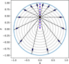 |
Fig. 1 Schematic diagram of the radiative transfer of hydrogen RRLs and continuum emission in the new model. The large blue circle shows the boundary of the spherical H II region. The blue asterisks represent the grid points for which the mean incident radiation field needs to be calculated. The dashed black lines show the radiation transfer paths in different directions. The arrows indicate the direction of propagation of the RRLs and the continuum emission. R and Z are the normalized radial and axial coordinates in the axisymmetric coordinate system. |
2.5 Simplifications in the radiative transfer treatment of the new model
In order to improve the computation speed of the new model, several simplifications were made in the treatment of radiative transfer. First, only the hydrogen RRLs with the difference between the upper and lower levels Δn = m – n ≤ 10 or with the lower level n ≤ 10 are calculated. This is easy to understand because the RRLs with Δn > 10 are always very weak, so that they do not affect the level populations. The spontaneous transition probability Am,n first decreases and then increases when n decreases from m–1 to 1 if m ≫ 1 (Brocklehurst 1971). RRLs with lower level n ≤ 10 are therefore included in the calculations, although these lines affect the results only very little. The results with/without this simplification in the EPA model are compared and shown in Fig. 2, and the differences are negligible. The reliability in the new model cannot be verified without excessive computation, and we therefore used the EPA model. Although the two models differ in their treatment of radiative transfer, the effects of the simplification are similar. Thus, it is appropriate to apply this simplification to the new model.
Second, when treating the radiative transfer of hydrogen RRLs, we used departure coefficients bn with the principal quantum number n and the spontaneous transition probability Am,n instead of bnl and Aml′,nl. The value of bn was derived from
 (18)
(18)
The values of bnl were calculated with the level population equations. The average spontaneous transition probability Am,n from the states of principal quantum number m to those of n is
 (19)
(19)
Then, Eqs. (6) and (9) can be simplified as
 (20)
(20)
and
 (21)
(21)
where Bmn can be derived from Amn (Peters et al. 2012).  is the line absorption coefficient under the LTE assumption. βn,m is the amplification coefficient, with the upper and lower level m and n given by (Gordon & Sorochenko 2002; Peters et al. 2012)
 (22)
(22)
In order to determine whether this simplification is reliable, we compared the results derived from the simplified model with those from the unsimplified model. The examples in Fig. 3 show that the differences due to this simplification are negligible.
Fig. 1 shows that the radiative transfer of hydrogen RRLs and the continuum is calculated along several paths in the two-dimensional axisymmetric coordinate system. Although a greater number of paths in radiative transfer calculations yields more accurate results, we typically restricted the computation to 7 distinct paths at each spatial grid point and required a departure coefficient determination to optimize the computational efficiency. By comparing computational results obtained with different numbers of paths, we found that the inclusion of 7 distinct paths in the radiation transfer calculations achieved sufficient accuracy while maintaining computational feasibility. This is shown in the comparison of the results derived from the calculations with 7 and 15 paths presented in Fig. 4. We adopted these three simplifications in the radiative transfer when we calculated the departure coefficients with the improved model.
In addition, although different numbers of the grid points from the center to the boundary of a spherical H II region can be set in the current model, we always used 10 grid points here. The corresponding positions of these grid points are from 0.05R to 0.95R with an equal spacing of 0.1R, where R is the radius of the spherical HII region. The model with 20 grid points was also applied to some exemplar cases. The results are not significantly different.
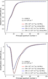 |
Fig. 2 Results calculated from the EPA models considering all hydrogen RRLs in the treatment of incident radiation fields, compared with those considering only relatively strong hydrogen RRLs. In the top panel, bn is plotted for different cases. βn,n+1 is presented in the bottom panel. |
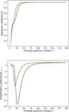 |
Fig. 3 Comparison of the results calculated from the improved new model with or without the second simplification described in Section 2.5. The solid red and yellow lines show the results calculated without the simplification for Te = 10 000 K, ne = 106 cm–3, and EM=1010 cm–6 pc and Te = 10 000 K, ne = 107 cm–3, and EM=1011 cm–6 pc, respectively. The dashed and dash-dotted black lines are those calculated with the simplification for the corresponding cases. In the top panel, we plot bn at the center of uniform spherical H II regions. βn,n+1 is presented in the bottom panel. |
2.6 Instability in calculations with extremely high EM
The emission measure (EM) is a measure of the ionized mass of a nebula that emits free-free radiation (Gordon & Sorochenko 2002). It is commonly defined as  with the line-of-sight (LOS) path s. The EPA model becomes unstable when the EM is very high (Prozesky & Smits 2020). This problem also appears in the current model with a full radiative transfer treatment. Following the smoothing method used by Prozesky & Smits (2020), we smoothed the values of the intensity Jv in adjacent steps. The smoothed intensity of the incident radiation field
  at the step t is given by
 (23)
(23)
where Jv,k is the Jv at the step k. k means the sequence number of iterations. p is the number of adjacent steps required for the smoothing. The value of p was set to be 3–5 in most cases and to 10 when the EM was extremely high for a given Te and ne. The smoothing method is useful for stabilizing the calculations in some cases with high EMs. The calculation might still break down when the EM exceeds a limit for given Te and ne. Compared with the available observations (Wood & Churchwell 1989; De Pree 2020; Báez-Rubio et al. 2013; Sánchez Contreras et al. 2019), the roughly estimated EMs corresponding to Te and ne in the U/HC H II regions are within the limits of the current models.
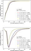 |
Fig. 4 Comparison of the results calculated with the improved new model in which radiative transfer is treated along 7 and 15 paths for some exemplary cases. In the top panel, we plot bn at the center of uniform spherical H II regions. The correspondingis βn,n+1 is presented in the bottom panel. |
3 Results and discussions
In this section, we compare the results calculated using the models without effects of radiation fields (Zhu et al. 2019), with the escape probability approximation (Zhu et al. 2022), and with the full radiative transfer treatment. We investigate the appropriate conditions for the previous models, and we study the advantage of the improved current model. We create a machine-learning model based on the current model and the EPA model.
The current model can handle spherically symmetric H II regions with density gradients and radial velocities. To enable a comparison with the EPA model, which is only applicable to homogeneous targets, all cases we simulated were uniform spherical H II regions. For these cases, the EM was defined to be  with the diameter of an H II region D. The Lyman-continuum photon production rate for an ionizing source in an H II region was assumed to be lower than 1.5 × 1050 s–1. This value corresponds to the rate of a young massive star cluster (Nguyen-Luong et al. 2017; Zhu et al. 2022). This allowed us to limit the strengths of the simulated radiation fields to an appropriate range. The ionized helium-to-hydrogen ratio Y+ was always equal to 0.1.
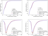 |
Fig. 5 Comparison of the results calculated from the improved current model with the full radiative transfer treatment and the EPA models with different escape probabilities. In the top panel, we compare bn at the center and boundary of uniform spherical H II regions in the current model with the EPA models with different escape probabilities. The corresponding βn,n+1 is presented in the bottom panel. |
3.1 Modification of the escape probability in the EPA model
The escape probability of  we used in the EPA model was that from Prozesky & Smits (2020). τν = κνL is the optical depth of a homogeneous medium of thickness L. For a uniform spherical H II region, the optical depth is τν = κνD. Following Prozesky & Smits (2020), this assumption was also applied to the EPA model in our previous work (Zhu et al. 2022). By comparing the results calculated from the current improved model and the EPA model, however, we found that τν = κνD/2 is more appropriate, as shown in Fig. 5. This is easy to understand because the mean incident radiation field in the EPA model with τν = κνD/2 is approximately equal to the field at the center of the spherical H II region when the departure coefficients at different locations in the H II region are not significantly different. The escape probability of
  with τν = κνD/2 is consistent with that used by Kegel (1979) and Koepen & Kegel (1980) for the CO and OH lines.
3.2 Spatial variations in the departure coefficients under different EM conditions within H II regions
When the radiation field is weak, the level populations of hydrogen atoms in H II regions are dominantly determined by the electron temperature and density (Storey & Hummer 1995; Zhu et al. 2022). In this case, there is no significant difference between the departure coefficients in the inner and in the boundary region. With increasing EM, the effects of radiation fields from RRLs and continuum emission increase gradually. The spatial variations in the departure coefficients within the H II regions become increasingly significant. In the top and middle panels of Fig. A.1, we present the departure coefficients bn calculated using different models for the cases with different EMs. The differences between bn derived using different models increase with the EM value. The results in the Case B model are significantly different from those in the other two models when the EM is high. The differences between bn in the center and boundary of the H II region are presented in the bottom panel. The spatial variations in the departure coefficients within the H II region increase with the EM, except at a few levels.
The corresponding comparisons for amplification coefficients βn,n+1 are shown in Fig. A.2. The differences in the results between different models are clearer in the comparisons of βn,n+1. The difference of the βn,n+1 calculated with the EPA model and the current model is more significant in the case of EM= 6 × 1011 cm–6 pc than that in the case of EM= 2 × 1011 cm–6 pc. In the bottom panel, the difference between βn,n+1 in the center and at the boundary of a spherical H II region is displayed for the cases of EM= 2 × 1011 cm–6 pc and 6 × 1011 cm–6 pc. It demonstrates that βn,n+1, and correspondingly, bn, at different positions vary more strongly for a higher EM. In addition, the top and middle panels show that the effects of radiation fields on hydrogen-level populations weaken the population inversion in the center and increase on either side of the valley of βn,n+1. The relevant detailed explanation of this phenomenon was presented by Zhu et al. (2022).
The luminosities of Hnα lines were calculated using the three models for the two cases of different EMs, but with the same Te and ne. The comparative differences between the Case B and EPA models relative to the current model are illustrated in Fig. A.3. In the two cases, the luminosities simulated using the Case B model are both much different from those calculated using the other models. The differences of the Hnα line luminosities between the EPA model and the current model are all smaller than 10% in the case of EM= 2 × 1011 cm–6 pc, but the differences become more significant in the case of EM= 6 × 1011 cm–6 pc.
The comparison of the two cases with different EMs and an identical temperature and density clearly shows that the spatial variations in the departure coefficients within the H II regions increase with the EM. Although we present only the cases of Te = 10 000 K and ne = 107 cm–3, the trend persists under other conditions. This is easy to understand. Different from the continuum emission, the intensity of stimulated emission strongly depends on the propagation path when the optical depth τ < – 1 because the EM is high. Consequently, the incident radiation field differs more strongly for the center and boundary of an HII region with higher EM.
3.3 Spatial variations in bn under different ne conditions
We plot the amplification coefficients βn,n+1 with the principal quantum number n calculated using the three models in Fig. A.4 for the case of Te = 10 000 K, ne = 5 × 106 cm–3, and EM= 2 × 1011 cm–6 pc. Compared to the results in the case of identical Te and EM, but ne = 107 cm–3 shown in the top panel of Fig. A.2, the discrepancies in βn,n+1 between the EPA and current models are more pronounced when the electron density is lower. Fig. A.5 also shows that the differences in the Hnα line luminosities between the EPA and the current models in the case of ne = 5 × 106 cm–3 are more distinct than those in the case of ne = 107 cm–3 mentioned above. The reason is that the absolute values of the line optical depths  of the masing Hnα lines are higher in the case of lower ne, so that the nonisotropic stimulated emission is more powerful.
3.4 Spatial variations in bn under different Te conditions
A similar trend also appears for a low temperature. The results in the case of Te = 6000 K, ne = 107 cm–3, and EM= 1011 cm–6 pc are shown in Fig. A.6. Compared with the cases of Te = 10 000 K and ne = 107 cm–3, the absorption coefficients κv,C and  are higher for low Te. This leads to higher absolute values of τν for masing lines. The top panel of Fig. A.6 shows that although the valley of βn,n+1 is shallower for Te = 6000 K, the higher |τν| for masing lines causes the stimulated emission to be powerful enough to significantly alter the amplification coefficients in the center of H II region from those in the boundary of the HII region even when EM is 1011 cm–6 pc.
The differences in the line luminosities between different models are presented in the bottom panel of Fig. A.6. The difference between the EPA model and the current model is clearly higher than that in the case of Te = 10 000 K, ne = 107 cm–3, and EM=2 × 1011 cm–6 pc for most millimeter Hnα lines.
3.5 Effects of the microturbulent velocity field
The line profile function of a hydrogen RRL is affected by the microturbulent velocity field (Peters et al. 2012). In the previous work (Zhu et al. 2022), we found that the importance of the stimulated emission decreases with the increasing root mean square συ of the microturbulent velocity field. Consequently, the differences between the results in the EPA and current models decrease with increasing συ. This is corroborated by the results shown in Fig. A.7, in which we show the amplification coefficients βn,n+1 and Hnα line luminosities in the case of Te = 10 000 K, ne = 107 cm–3, EM= 6 × 1011 cm–6 pc and the root mean square συ = 0 km s–1 and 20 km s–1. The difference between the results calculated in the EPA model and the current model is lower in the case of higher συ. The bottom panel of Fig. A.7 shows, however, that the difference of line intensities is still significant even in the case of συ = 20 km s–1 under the condition of a strong stimulated emission.
3.6 Appropriate ranges of previous models
In this section, we investigate the appropriate ranges of Te, ne, and EM for the Case B model and the EPA model for uniform spherical UC and HC H II regions. We adopted the classification standard for H II regions listed by de la Fuente et al. (2020) to classify UC H II regions (ne ≥ 104 cm–3 and EM≥ 107 cm–6 pc) and HC H II regions (ne ≥ 106 cm–3 and EM≥ 1010 cm–6 pc).
3.6.1 Case B model
The differences between the luminosities of the H20α, H25α, H30α, H35α, and H40α lines derived using the current model and the Case B model for UC and HC H II regions are shown in Tables 1 and 2, respectively. These millimeter hydrogen RRLs were used to present the differences between different models because hydrogen RRL masers that can significantly affect the hydrogen-level populations were detected in millimeter wavelengths (Martín-Pintado et al. 1989). As mentioned above, the Lyman-continuum photon production rate for an ionizing source in an H II region is assumed to be lower than 1.5 × 1050 s–1. The upper limit of the EM was derived with a given Te and ne. We therefore did not calculate the cases with an EM higher than the upper limit.
Table 1 shows that the differences between the line luminosities using the two models are smaller than 10% for UC H II regions with Te = 6000 K and 10 000 K. If a difference lower than 10% is thought to be insignificant, the Case B model is accurate enough for calculating the hydrogen RRLs in UC H II regions. The differences between the two models for the HC H II regions are presented in Table 2. The Case B model is only appropriate for a small fraction of cases with a relatively low EM ~1010 cm–6 pc for the HC H II regions.
Prozesky & Smits (2018) implied that the Case B model was unsuitable for UC H II regions because the effect of free-free continuum radiation on hydrogen-level populations becomes significant for ne > 104 cm–3. The results we show in Table 1 and Table 2 indicate, however, that the Case B model is suitable for simulating hydrogen RRLs in UC H II regions, but it probably deviates substantially for HC H II regions.
Differences between the luminosities of the Hnα lines calculated using the current model and the Case B model for a uniform spherical UC H II region with various Te, ne, and EM.
Differences between luminosities of the Hnα lines calculated using the current model and the Case B model for a uniform spherical HC H II region with various Te, ne, and EM.
3.6.2 EPA model
We list the differences between the line luminosities calculated using the current model and the EPA model for HC H II regions in Table 3. As mentioned in Sections 3.2, 3.3, and 3.4, the differences increase with the EM and decrease with Te and ne. The conditions under which the results calculated by the two models are significantly different are shown. Although only the results for a few cases are listed, we also calculated cases with other values of Te, ne, and EM. According to the results, the EPA model is not accurate enough in the cases of EM > EMcrt for a given Te and ne. The value of EMcrt can be roughly estimated by an empirical formula as
 (24)
(24)
where Te, ne, and EM are in units of K, cm–3, and cm–6 pc, respectively.
Compared with the estimated values of Te, ne, and EM in previous observations toward HC H II regions, this seems to suggest that the EPA model is appropriate for most HC H II regions if these H II regions can be treated as a uniform and spherical region (Murphy et al. 2010; De Pree 2020). For rare objects with clearly detected hydrogen recombination line masers (e.g., MWC349 and MWC922), however, the EPA model becomes inadequate because their EMs are extremely high (Báez-Rubio et al. 2013; Sánchez Contreras et al. 2019; De Pree 2020; Martínez-Henares et al. 2023), even when the density gradients in these sources are not accounted for.
Differences between luminosities of the Hnα lines calculated using the current model and the EPA model for a uniform spherical HC H II region with various Te, ne, and EM.
3.7 Advantage of the current model with a full radiative transfer treatment
In Section 3.6, we studied the appropriate ranges of the Case B model and the EPA model. The Case B model and the EPA model are suitable for UC H II regions and other classes of H II regions with lower ne and EM. The EPA model is appropriate for estimating the global properties of most cases of HC H II regions with EM<EMcrt. For HC H II regions with EM≥EMcrt, the current model is necessary. Furthermore, in modeling the 2D observational images of the hydrogen RRLs from HC H II regions, the superiority of the current model over the EPA model becomes more pronounced because the EPA model was primarily designed to simulate global-scale properties of an H II region (Prozesky & Smits 2020).
3.8 Machine-learning model for uniform spherical H II regions
Calculations of departure coefficients of hydrogen-level populations are often time-consuming. Especially for the current model with its full radiative transfer, the calculation time can sometimes reach several days. This motivated us to train a machine-learning model to accelerate the calculation of the departure coefficients. We employed the random forest algorithm, which is a powerful ensemble-learning method that is widely used in various fields (Breiman 2001). It combines multiple decision trees to improve the predictive performance. Each tree is built using a random subset of the training data and a random selection of features, which reduces overfitting and correlation among the trees. The final prediction is derived by aggregating the predictions of all trees.
Our training and validation data consisted of the data simulated by using the current and EPA models. In a sample of the dataset, the values of Te, log(ne), log(EM), and συ were the inputs, and βn,n+1 with the principal quantum number n in the range of 3 to 200 and b200 were the outputs. The departure coefficients bn in the corresponding levels n were derived from the values of βn,n+1 and b200 with Te.
3.8.1 Mock data and parameter settings for the machine-learning model
In the dataset, the ranges of Te, ne, EM, and συ were 5000–15 000 K, 102–108 cm–3, ≤ 1012 cm–6 pc, and ≤ 50 km s–1, respectively. The value of EM was also limited by a reasonable Lyman-continuum photon production rate <1.5 × 1050 s–1 for a spherical H II regionwith agiven Te and ne. The value of Y+ was assumed to be 0.1. According to the values of Te, ne, and EM, the total dataset was divided into three subsets, as listed in Table 4. These three subsets included 12 168 samples with ne < 104 cm–3, 401335 samples with ne ≥ 104 cm–3 and EM≲ 0.5EMcrt, and 39 292 samples of ne ≥ 104 cm–3 and EM≥ 0.5EMcrt, respectively. The data in subsets 1 and 2 were calculated by the EPA model, and those in subset 3 were simulated by the current model with a full radiative transfer treatment. Then, the total machine-learning model was composed of three submodels corresponding to the three subsets. For each submodel, the data in the subset were divided into a training and a testing set with a ratio of 8 to 2. The former set was used to train the predictive model, and the latter was used to assess the performance of that model. The function of the random forest regressor1 was used. The parameters set in this function are as follows. The number of trees was 100, the maximum depth of the tree was set to be 13, the minimum number of samples required to split an internal node was 2, and the minimum number of samples required to be at a leaf node was 1.
The electron temperature, density-EM, and συ distributions of the samples in the three subsets are shown in Fig. A.8. The temperature distributions are plotted in the top panels. The distribution for the samples of ne < 104 cm–3 is relatively uniform. There are relatively fewer samples with a high temperature in the other two subsets because the effects of radiation fields are stronger for the cases with a low temperature, so that more samples are needed for the machine-learning model to reach accurate predictions. The electron density-EM distributions are presented in the middle panels. The ne-EM distributions in the samples are more inhomogeneous than the temperature distributions. For the cases of ne < 104 cm–3, the effects of radiation fields due to continuum emission and RRLs on departure coefficients can be neglected, as shown in Section 3.6. The samples are mainly distributed in EM= 20 cm–6 pc and 2.0 × 107 cm–6 pc in the corresponding subset. The value of bn with EM between the two values can be correctly predicted since the different values of EM have negligible effects on the departure coefficients for the cases with EM<1010 cm–6 pc. In the second subset, a large part of the samples is distributed in the range of EM > 109 cm–6 pc because the departure coefficients are sensitive to the value of the EM when the EM is close to EMcrt. More samples are necessary to be recorded for these cases. This type of treatment is also shown in the ne-EM distributions of the third subset plotted in the middle right panel. The συ distributions are presented in the bottom panels of Fig. A.8. The distribution for the first subset is not plotted. The effects of the radiation fields are not significant in the cases of ne < 104 cm–3, and we therefore assumed all values of συ to be 0 km s–1.
Classification of subsets in the total dataset. The EM was also limited by the Lyman-continuum photon production rate < 1.5 × 1050 s–1 for an H II region.
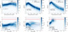 |
Fig. 6 Validation results of the machine-learning model for the testing set. The results of the three submodels corresponding to different subsets are presented in the left, middle, and right panels, respectively. The comparisons of the departure coefficients calculated by the simulation models and the machine-learning submodels are presented in the top panels. In the bottom panels, we show the comparisons of the Hnα line luminosities. Lm and Ls denote the line luminosities computed using the departure coefficients from the machine-learning model predictions and the original simulation models, respectively. The solid and dashed red lines in the bottom panels correspond to error levels of 10% and 20%, respectively. |
3.8.2 Validation results of the machine-learning model
The validation results of the testing sets are presented in Fig. 6. The predicted and true values are very close. The top panels of Fig. 6 show that the absolute differences between the departure coefficients |Δbn| calculated by the numerical models and predicted by the machine-learning model are mostly lower than 0.001. bn is very close to 1 at the high principal quantum number n when the electron density ne is high (Brocklehurst 1970; Storey & Hummer 1995; Prozesky & Smits 2018; Zhu et al. 2022). This causes the absolute errors of bn with high n in the testsets of subsets 2 and 3 to be far smaller than those of subset 1.
We compare the Hnα line luminosities calculated using bn from the simulation models and the machine-learning model in the bottom panels of Fig. 6. Cases with a continuum optical depth τv,C > 3 were not taken into account because practical observational strategies for hydrogen RRLs typically avoid such high τv,C. The bottom right panel for subset 3 therefore shows no results for Hnα lines with n > 50. For subsets 1 and 2, the difference in the Hnα line luminosity is always lower than 1%. For subset 3, the difference is lower than 10% in most cases, although the difference can be higher in some conditions. This might result from the fewer samples in subset 3 than in subset 2. In summary, the illustrations presented in Fig. 6 demonstrate that the machine-learning model achieves sufficient accuracy to substitute the numerical models for most spherical H II regions. The machine-learning model and its datasets are available for download2.
4 Summary and conclusions
We improved our previous EPA model, a new nl-model with the full radiative transfer treatment about hydrogen RRLs and continuum emission for spherical H II regions. The departure coefficients in different locations within H II regions were calculated meticulously.
The appropriate ranges of the Case B model and the EPA model were studied by comparing them with the new model. The effects of radiation fields on the departure coefficients can be neglected for classical and UC H II regions (ne < 106 cm–6 and EM < 109 cm–6 pc). With the appropriately modified escape probability, the EPA model was proven to be suitable for most cases of HC H II regions in which the EM is lower than the critical value of EM (EMcrt). By comparing the intensities of hydrogen RRLs calculated using the EPA model and the current model, we estimated the EMcrt as a function of a given Te and ne of a uniform and spherical H II region. Compared with our previous models, the new model has a significant advantage for HC H II regions with extremely high EMs that are higher than EMcrt.
Based on a large sample of departure coefficients calculated with the EPA model and the current model, we created an accurate machine-learning model to quickly estimate the departure coefficients and resulting properties of hydrogen RRLs from the electron temperature, number density, EM, and the root mean square of the microturbulent velocity field of a spherical H II region. We applied the random forest algorithm. The differences between the departure coefficients predicted by the machine-learning model and the simulation model are mostly lower than 0.001.
Acknowledgements
The authors thank the anonymous referee for the detailed comments to improve the quality of the manuscript. The work is supported by the National Natural Science Foundation of China No. 12373026, the Leading Innovation and Entrepreneurship Team of Zhejiang Province of China No. 2023R01008, the Key R&D Program of Zhejiang, China No. 2024SSYS0012, and Zhejiang Provincial Natural Science Foundation of China No. LY24A030001.
Appendix A Additional figures
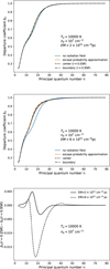 |
Fig. A.1 The comparison of the calculated departure coefficients bn with principal quantum number n using the Case B model (blue), the EPA model (red), and the current model with full radiative transfer (black). The dashed and dash-dotted lines respectively indicate the values at the locations 0.05R (center) and 0.95R (boundary) distant from the central massive star in the spherical H II region. R is the radius of a spherical H II region. The electron temperature and density of the H II region are 10000 K and 107 cm–3. The results for EM = 2 × 1011 cm–6 pc and EM = 6 × 1011 cm–6 pc are shown in the top and middle panels, respectively. The differences between bn in the center and the boundary of H II regions of the corresponding EMs are plotted in the bottom panel. |
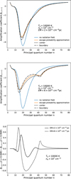 |
Fig. A.2 The comparison of the calculated amplification coefficients βn,n+1 using the Case B model, the EPA model, and the current model. The electron temperature and density of the H II region are 10000 K and 107 cm–3. The values of EM are 2 × 1011 cm–6 pcand 6 × 1011 cm–6 pc for the cases shown in the top and middle panels, respectively. The differences between βn,n+1 in the center and the boundary of H II regions of the corresponding EMs are plotted in the bottom panel. |
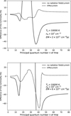 |
Fig. A.3 The difference between the luminosities of Hnα lines calculated using the Case B model, the EPA model, and the current model. Curves labeled “no radiation field/current” correspond to differential luminosities derived by subtracting our current model values from Case B model results, while those marked “EPA/current” show analogous comparisons between the EPA model and the current model. |
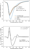 |
Fig. A.4 The comparison of the calculated amplification coefficients βn,n+1 using the Case B model, the EPA model, and the current model. The electron temperature and density of the H II region are 10000 K and 5 × 106 cm–3. The values of EM are 2 × 1011 cm–6 pc. The differences between βn,n+1 in the center and the boundary of H II regions in this case are plotted in the bottom panel, in comparison with those in the case of Te = 10000 K, ne = 5 × 106 cm–3 and EM= 2 × 1011 cm–6 pc. |
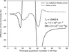 |
Fig. A.5 The differences between the luminosities of Hnα lines calculated using the Case B model, the EPA model, and the current model. |
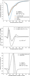 |
Fig. A.6 The comparison of the calculated amplification coefficients βn,n+1 using the Case B model, the EPA model, and the current model with full radiative transfer is plotted in the top panel. The electron temperature and density of the H II region are 6000 K and 107 cm–3. The value of EM is 1011 cm–6 pc. The differences between βn,n+1 in the center and the boundary of H II regions in two cases of identical ne but different Te and EM are plotted in the middle panel. In the bottom panel, the differences between the luminosities of Hnα lines calculated using the Case B model, the EPA model and the current model for the case of Te = 6000 K, ne = 107 cm–3, and EM= 1011 cm–6 pc are presented. |
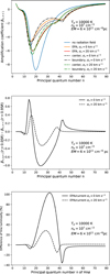 |
Fig. A.7 The comparison of the calculated amplification coefficients βn,n+1 using the EPA model and the current model with full radiative transfer is plotted in the top panel. The corresponding comparisons of the βn,n+1 in the center and boundary of H II regions, and the line luminosities are shown in the middle and bottom panels, respectively. The electron temperature, density and EM are 10000 K, 107 cm–3, and 6 × 1011 cm–6 pc, respectively. The συ is 0 km s–1 and 20 km s–1 in the two cases. |
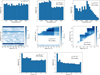 |
Fig. A.8 The temperature, electron density-EM, and συ distributions. The temperature distributions in the three subsets of samples are presented in the top panels. The density-EM distributions are shown in the middle panels. The distributions of συ in the two subsets including samples of ne ≥ 104 cm–3 are plotted in the bottom panels. |
References
- Afflerbach, A., Churchwell, E., Hofner, P., & Kurtz, S. 1994, ApJ, 437, 697 [NASA ADS] [CrossRef] [Google Scholar]
- Arthur, S. J., & Hoare, M. G. 2006, ApJS, 165, 283 [NASA ADS] [CrossRef] [Google Scholar]
- Baker, J. G., & Menzel, D. H. 1938, ApJ, 88, 52 [Google Scholar]
- Báez-Rubio, A., Martín-Pintado, J., Thum, C., & Planesas, P. 2013, A&A, 553, A45 [NASA ADS] [CrossRef] [EDP Sciences] [Google Scholar]
- Breiman, L. 2001, Mach. Learn., 45, 5 [Google Scholar]
- Brocklehurst, M. 1970, MNRAS, 148, 417 [NASA ADS] [CrossRef] [Google Scholar]
- Brocklehurst, M. 1971, MNRAS, 153, 471 [Google Scholar]
- Burgess, A., & Summers, H. P. 1976, MNRAS, 174, 345 [Google Scholar]
- Churchwell, E., & Walmsley, C. M. 1975, A&A, 38, 451 [NASA ADS] [Google Scholar]
- Dieter, N. H. 1967, ApJ, 150, 435 [Google Scholar]
- Deharveng, L., Schuller, F., Anderson, L. D., et al. 2010, A&A, 523, A6 [NASA ADS] [CrossRef] [EDP Sciences] [Google Scholar]
- De Pree, C. G., Wilner, D. J., Kristensen, L. E., et al. 2020, AJ, 160, 234 [Google Scholar]
- Dumont, A.-M., Collin, S, Paletou, F., 2003, A&A, 407, 13 [NASA ADS] [CrossRef] [EDP Sciences] [Google Scholar]
- de la Fuente, E., Tafoya, D., Trinidad, M. A., et al. 2020, MNRAS, 497, 4436 [NASA ADS] [CrossRef] [Google Scholar]
- Gordon, M. A., & Sorochenko, R. L. 2002, Radio Recombination Lines (Berlin: Springer) [Google Scholar]
- Hummer, D. G., & Storey, P. J. 1987, MNRAS, 224, 801 [NASA ADS] [CrossRef] [Google Scholar]
- Kegel, W. H. 1979, A&AS, 38, 131 [NASA ADS] [Google Scholar]
- Koeppen, J., & Kegel, W. H. 1980, A&AS, 42, 59 [NASA ADS] [Google Scholar]
- Martín-Pintado, J., Bachiller, R., Thum, C., & Walmsley, C. M. 1989, A&A, 215, L13 [Google Scholar]
- Martínez-Henares, A., Jiménez-Serra, I., Martín-Pintado, J., Huélamo, N., & Prasad, S. 2023, ApJ, 955, 119 [CrossRef] [Google Scholar]
- Mezger, P. G., & Höglund, B. 1967, ApJ, 147, 579 [Google Scholar]
- Murphy, T., Cohen, M., Ekers, R. D., et al. 2010, MNRAS, 405, 1560 [Google Scholar]
- Nesterenok, A. V. 2016, MNRAS, 455, 3978 [Google Scholar]
- Nguyen-Luong, Q., Anderson, L. D., Motte, F., et al. 2017, ApJ, 844, 25 [NASA ADS] [CrossRef] [Google Scholar]
- Oster, L. 1961, RvMP, 33, 525 [NASA ADS] [Google Scholar]
- Peters, T., Longmore, S. N., & Dullemond, C. P. 2012, MNRAS, 425, 2352 [NASA ADS] [CrossRef] [Google Scholar]
- Prozesky, A., & Smits, D. P. 2018, MNRAS, 478, 2766 [NASA ADS] [CrossRef] [Google Scholar]
- Prozesky, A., & Smits, D. P. 2020, MNRAS, 491, 2536 [NASA ADS] [Google Scholar]
- Salgado, F., Morabito, L. K., Oonk, J. B. R., et al. 2017, ApJ, 837, 141 [Google Scholar]
- Sánchez Contreras, C., Báez-Rubio, A., Alcolea, J., Castro-Carrizo, A., & Bujarrabal, V. 2019, A&A, 629, A136 [NASA ADS] [CrossRef] [EDP Sciences] [Google Scholar]
- Sejnowski, T. J., & Hjellming, R. M. 1969, ApJ, 156, 915 [NASA ADS] [CrossRef] [Google Scholar]
- Shaver, P. A., McGee, R. X., Newton, L. M., Danks, A. C., & Pottasch, S. R. 1983, MNRAS, 204, 53 [NASA ADS] [CrossRef] [Google Scholar]
- Storey, P. J., & Hummer, D. G. 1995, MNRAS, 272, 41 [NASA ADS] [CrossRef] [Google Scholar]
- Sorochenko, R. L., & Borodzich, E. V. 1966, Sov. Phys.-Dokl., 10, 588 [Google Scholar]
- Townsley, L., Feigelson, E. D., Montmerle, T., et al. 2003, ApJ, 593, 874 [NASA ADS] [CrossRef] [Google Scholar]
- Walmsley, C. M. 1990, A&AS, 82, 201 [NASA ADS] [Google Scholar]
- Wood, D. O. S., & Churchwell, E. 1989, ApJS, 69, 831 [Google Scholar]
- Zhang, C., Evans II, N. J., Liu, T., et al. 2022, MNRAS, 510, 4998 [NASA ADS] [CrossRef] [Google Scholar]
- Zhang, C., Zhu, F.-Y., Liu, T., et al. 2023, MNRAS, 520, 3245 [NASA ADS] [CrossRef] [Google Scholar]
- Zhu, F.-Y., Zhu, Q.-F., Wang, J.-Z., & Zhang, J.-S. 2019, ApJ, 881, 14 [NASA ADS] [CrossRef] [Google Scholar]
- Zhu, F.-Y., Wang, J. Z., Zhu, Q.-F., & Zhang, J.-S. 2022, A&A, 665, A94 [NASA ADS] [CrossRef] [EDP Sciences] [Google Scholar]
- Zhu, F.-Y., Wang, J., Yan, Y., Zhu, Q.-F., & Li, J. 2023, MNRAS, 522, 503 [Google Scholar]
All Tables
Differences between the luminosities of the Hnα lines calculated using the current model and the Case B model for a uniform spherical UC H II region with various Te, ne, and EM.
Differences between luminosities of the Hnα lines calculated using the current model and the Case B model for a uniform spherical HC H II region with various Te, ne, and EM.
Differences between luminosities of the Hnα lines calculated using the current model and the EPA model for a uniform spherical HC H II region with various Te, ne, and EM.
Classification of subsets in the total dataset. The EM was also limited by the Lyman-continuum photon production rate < 1.5 × 1050 s–1 for an H II region.
All Figures
|
Fig. 1 Schematic diagram of the radiative transfer of hydrogen RRLs and continuum emission in the new model. The large blue circle shows the boundary of the spherical H II region. The blue asterisks represent the grid points for which the mean incident radiation field needs to be calculated. The dashed black lines show the radiation transfer paths in different directions. The arrows indicate the direction of propagation of the RRLs and the continuum emission. R and Z are the normalized radial and axial coordinates in the axisymmetric coordinate system. |
| In the text | |
|
Fig. 2 Results calculated from the EPA models considering all hydrogen RRLs in the treatment of incident radiation fields, compared with those considering only relatively strong hydrogen RRLs. In the top panel, bn is plotted for different cases. βn,n+1 is presented in the bottom panel. |
| In the text | |
|
Fig. 3 Comparison of the results calculated from the improved new model with or without the second simplification described in Section 2.5. The solid red and yellow lines show the results calculated without the simplification for Te = 10 000 K, ne = 106 cm–3, and EM=1010 cm–6 pc and Te = 10 000 K, ne = 107 cm–3, and EM=1011 cm–6 pc, respectively. The dashed and dash-dotted black lines are those calculated with the simplification for the corresponding cases. In the top panel, we plot bn at the center of uniform spherical H II regions. βn,n+1 is presented in the bottom panel. |
| In the text | |
|
Fig. 4 Comparison of the results calculated with the improved new model in which radiative transfer is treated along 7 and 15 paths for some exemplary cases. In the top panel, we plot bn at the center of uniform spherical H II regions. The correspondingis βn,n+1 is presented in the bottom panel. |
| In the text | |
|
Fig. 5 Comparison of the results calculated from the improved current model with the full radiative transfer treatment and the EPA models with different escape probabilities. In the top panel, we compare bn at the center and boundary of uniform spherical H II regions in the current model with the EPA models with different escape probabilities. The corresponding βn,n+1 is presented in the bottom panel. |
| In the text | |
|
Fig. 6 Validation results of the machine-learning model for the testing set. The results of the three submodels corresponding to different subsets are presented in the left, middle, and right panels, respectively. The comparisons of the departure coefficients calculated by the simulation models and the machine-learning submodels are presented in the top panels. In the bottom panels, we show the comparisons of the Hnα line luminosities. Lm and Ls denote the line luminosities computed using the departure coefficients from the machine-learning model predictions and the original simulation models, respectively. The solid and dashed red lines in the bottom panels correspond to error levels of 10% and 20%, respectively. |
| In the text | |
|
Fig. A.1 The comparison of the calculated departure coefficients bn with principal quantum number n using the Case B model (blue), the EPA model (red), and the current model with full radiative transfer (black). The dashed and dash-dotted lines respectively indicate the values at the locations 0.05R (center) and 0.95R (boundary) distant from the central massive star in the spherical H II region. R is the radius of a spherical H II region. The electron temperature and density of the H II region are 10000 K and 107 cm–3. The results for EM = 2 × 1011 cm–6 pc and EM = 6 × 1011 cm–6 pc are shown in the top and middle panels, respectively. The differences between bn in the center and the boundary of H II regions of the corresponding EMs are plotted in the bottom panel. |
| In the text | |
|
Fig. A.2 The comparison of the calculated amplification coefficients βn,n+1 using the Case B model, the EPA model, and the current model. The electron temperature and density of the H II region are 10000 K and 107 cm–3. The values of EM are 2 × 1011 cm–6 pcand 6 × 1011 cm–6 pc for the cases shown in the top and middle panels, respectively. The differences between βn,n+1 in the center and the boundary of H II regions of the corresponding EMs are plotted in the bottom panel. |
| In the text | |
|
Fig. A.3 The difference between the luminosities of Hnα lines calculated using the Case B model, the EPA model, and the current model. Curves labeled “no radiation field/current” correspond to differential luminosities derived by subtracting our current model values from Case B model results, while those marked “EPA/current” show analogous comparisons between the EPA model and the current model. |
| In the text | |
|
Fig. A.4 The comparison of the calculated amplification coefficients βn,n+1 using the Case B model, the EPA model, and the current model. The electron temperature and density of the H II region are 10000 K and 5 × 106 cm–3. The values of EM are 2 × 1011 cm–6 pc. The differences between βn,n+1 in the center and the boundary of H II regions in this case are plotted in the bottom panel, in comparison with those in the case of Te = 10000 K, ne = 5 × 106 cm–3 and EM= 2 × 1011 cm–6 pc. |
| In the text | |
|
Fig. A.5 The differences between the luminosities of Hnα lines calculated using the Case B model, the EPA model, and the current model. |
| In the text | |
|
Fig. A.6 The comparison of the calculated amplification coefficients βn,n+1 using the Case B model, the EPA model, and the current model with full radiative transfer is plotted in the top panel. The electron temperature and density of the H II region are 6000 K and 107 cm–3. The value of EM is 1011 cm–6 pc. The differences between βn,n+1 in the center and the boundary of H II regions in two cases of identical ne but different Te and EM are plotted in the middle panel. In the bottom panel, the differences between the luminosities of Hnα lines calculated using the Case B model, the EPA model and the current model for the case of Te = 6000 K, ne = 107 cm–3, and EM= 1011 cm–6 pc are presented. |
| In the text | |
|
Fig. A.7 The comparison of the calculated amplification coefficients βn,n+1 using the EPA model and the current model with full radiative transfer is plotted in the top panel. The corresponding comparisons of the βn,n+1 in the center and boundary of H II regions, and the line luminosities are shown in the middle and bottom panels, respectively. The electron temperature, density and EM are 10000 K, 107 cm–3, and 6 × 1011 cm–6 pc, respectively. The συ is 0 km s–1 and 20 km s–1 in the two cases. |
| In the text | |
|
Fig. A.8 The temperature, electron density-EM, and συ distributions. The temperature distributions in the three subsets of samples are presented in the top panels. The density-EM distributions are shown in the middle panels. The distributions of συ in the two subsets including samples of ne ≥ 104 cm–3 are plotted in the bottom panels. |
| In the text | |
Current usage metrics show cumulative count of Article Views (full-text article views including HTML views, PDF and ePub downloads, according to the available data) and Abstracts Views on Vision4Press platform.
Data correspond to usage on the plateform after 2015. The current usage metrics is available 48-96 hours after online publication and is updated daily on week days.
Initial download of the metrics may take a while.