| Issue |
A&A
Volume 701, September 2025
|
|
|---|---|---|
| Article Number | A95 | |
| Number of page(s) | 14 | |
| Section | Catalogs and data | |
| DOI | https://doi.org/10.1051/0004-6361/202555668 | |
| Published online | 04 September 2025 | |
Caveats about measuring carbon abundances in stars using the CH band
1
Departamento de Física de la Tierra y Astrofísica, Universidad Complutense de Madrid,
28040
Madrid,
Spain
2
Instituto de Física de Partículas y del Cosmos IPARCOS, Facultad de CC Físicas, Universidad Complutense de Madrid,
28040
Madrid,
Spain
3
Instituto de Astrofísica de Canarias,
38200
La Laguna,
Tenerife,
Spain
4
Departamento de Astrofísica, Universidad de La Laguna,
38205
Tenerife,
Spain
5
Université Côte d’Azur, Observatoire de la Côte d’Azur, CNRS, Laboratoire Lagrange,
France
6
Data Science Research Centre, Liverpool John Moores University,
Liverpool
L3 3AF,
UK
★ Corresponding author; This email address is being protected from spambots. You need JavaScript enabled to view it.
Received:
26
May
2025
Accepted:
14
July
2025
Abstract
Context. Stellar carbon abundances are crucial for tracing the star formation history and predicting the near-infrared emission of galaxies. It is still a complex task to derive accurate carbon abundance estimates for a wide variety of stars because it is hard to measure it based on atomic and molecular lines. It therefore remains challenging to include the abundance in stellar population models.
Aims. We analyse the carbon abundance determination for the large empirical X-shooter Spectral Library that is commonly used as a benchmark for the development of stellar population models.
Methods. We analysed the carbon abundance over strong molecular CH bands in the G-band region. We used the automated spectrum synthesis code GAUGUIN and adopted two different grids of separate reference synthetic spectra, each with the same coverage of the [C/Fe] abundance. We carried out a detailed comparison of the two grids to evaluate the accuracy and the model dependence of the measured [C/Fe] abundances.
Results. We obtained a large and precise unbiased [C/Fe] abundance catalogue (~200 stars) from the two theoretical grids, well distributed in the Hertzsprung-Russell diagram and with no a trend with the stellar parameters. We also measured compatible values from each independent CH band, with a high-quality [C/Fe] abundance estimate for both dwarfs and giants. We always observed a dispersed flat trend around [C/Fe] ~ 0.0 dex throughout the entire metallicity regime we covered (–5 < [Fe/H] < +0.5 dex). This agrees with some previous studies. However, we found variations up to |Δ[C/Fe]| ~ 0.8 dex in the [C/Fe] composition of the star depending on the adopted grid. We found no such difference in the α-element measurements. This behaviour implies that the [C/Fe] abundance estimate strongly depends on the model.
Conclusions. Potential sources of error might be associated with the use of spectral synthesis methods to derive stellar carbon abundances in the CH 4300 Å band. Intrinsic small differences in the synthetic models for this crowded and blended region may induce a large disparity in the precise abundance estimate for any stellar type, which leads to inadvertently inaccurate carbon measurements.
Key words: methods: data analysis / techniques: spectroscopic / stars: abundances
© The Authors 2025
 Open Access article, published by EDP Sciences, under the terms of the Creative Commons Attribution License (https://creativecommons.org/licenses/by/4.0), which permits unrestricted use, distribution, and reproduction in any medium, provided the original work is properly cited.
This article is published in open access under the Subscribe to Open model. This email address is being protected from spambots. You need JavaScript enabled to view it. to support open access publication.
Introduction
The chemical composition of stars is intimately linked to the star formation history (SFH) of galaxies and star clusters (e.g. Freeman & Bland-Hawthorn 2002; Harris & Zaritsky 2009; de La Rosa et al. 2011; Fernández-Alvar et al. 2018). While individual stellar abundances can be directly measured in the Milky Way and nearby galaxies, the properties of more distant systems must be inferred indirectly through models of stellar population synthesis (e.g. Bruzual & Charlot 2003; Mollá et al. 2009; Vazdekis et al. 2010; Maraston et al. 2020).
These models often rely on empirical stellar libraries that reflect the chemical abundance patterns of the Milky Way (e.g. Vazdekis 1999; Vazdekis et al. 2010, 2016; Bruzual & Charlot 2003; Le Borgne et al. 2004; Maraston & Strömbäck 2011; Maraston et al. 2020; Verro et al. 2022a), and the predictions are therefore linked to the specific star formation history of the solar neighbourhood. To accurately interpret the integrated light from external galaxies, however, models need to make predictions for well-defined abundance patterns that do not change with metallicity. A common approach to make these predictions is to apply theoretical corrections to the empirical spectra (e.g. Cervantes et al. 2007; Walcher et al. 2009; Conroy & van Dokkum 2012; Conroy et al. 2018; Vazdekis et al. 2015; La Barbera et al. 2016; Knowles et al. 2023) using the changes in the model atmosphere spectra when a single chemical element is changed. This approach means that the chemical abundances of the empirical stars must be known in the first place.
So far, carbon (C; Z = 6) has not been fully included in stellar population models because large empirical spectral libraries with reliable [C/Fe] measurements for a wide range of stellar parameters (Teff, log(g), [Fe/H]) are lacking, such as MILES (Sánchez-Blázquez et al. 2006), MEGASTAR (Carrasco et al. 2021), ELODIE (Prugniel & Soubiran 2001), or X-shooter (Chen et al. 2014; Arentsen et al. 2019; Gonneau et al. 2020; Verro et al. 2022b). Carbon1 is essential for understanding the early chemical enrichment of galaxies through contributions from massive stars and Type II supernovae, and later stages of stellar evolution, in particular by asymptotic giant branch (AGB) stars and binary interaction (see e.g. Frebel et al. 2007; Kobayashi et al. 2020).
Carbon-rich stars are found at all metallicities and in evolutionary stages, with a rising incidence at low metallicities, which is an important imprint of early star formation episodes (see e.g. Lebzelter et al. 2018; Sestito et al. 2024; Ardern-Arentsen et al. 2025). AGB stars (giants with low to intermediate masses of 1–8 M⊙) in particular dominate the near-infrared (NIR) emission in intermediate-age stellar populations, but theoretical predictions of their contribution remain uncertain (e.g. Baldwin et al. 2018; Dahmer-Hahn et al. 2018; Verro et al. 2022a) because the physics of mixing (dredge-ups, e.g. Iben 1965; Gallino et al. 1998), binarity, and mass loss (e.g. Cristallo et al. 2011; Karakas & Lattanzio 2014; Osborn et al. 2025) is complicated.
Additionally, there are persistent issues in NIR stellar population models. For instance, recent models are unable to reproduce the CO-strong feature that is observed in the spectra of early-type galaxies (see Eftekhari et al. 2022, and references therein). Moreover, there are still discrepancies between spectroscopic ages and those derived based on a colour–magnitude diagram (CMD) (so-called model zero-point problem, see e.g. Eftekhari et al. 2025). These issues further underscore the need for accurate carbon abundance data in empirical libraries.
Observationally, it remains challenging to determine [C/Fe]. The reported abundance values vary widely, depending on the spectral resolution, method, and the specific carbon features that are analysed. Most large surveys focus on FGK dwarfs (3500 ≲ Teff ≲ 7500 K; log(g) > 3.5 cm s–2) because their atmospheres are less strongly affected by internal mixing than those of giant stars (log(g) < 3.5 cm s–2) (e.g. Delgado Mena et al. 2010, 2021; Nissen et al. 2014; Franchini et al. 2020; Bensby et al. 2021).
The main goal of this work is to derive reliable [C/Fe] abundances for stars in the X-shooter Spectral Library (hereafter XSL; Arentsen et al. 2019; Gonneau et al. 2020), which is one of the most comprehensive currently available empirical stellar libraries with a resolution that is high enough to measure individual chemical abundances. We perform a detailed spectroscopic analysis of the CH molecular bands in the G-band region for a subsample of 611 stars from XSL (Santos-Peral et al. 2023). The structure of this paper is as follows: We describe in Sect. 2 the observational data, Sect. 3 details the spectral synthesis method and line selection, Sect. 4 presents the [C/Fe] measurements and their uncertainties, and Sect. 5 summarises our findings.
2 The X-shooter observational data sample
The XSL2 (Chen et al. 2014; Gonneau et al. 2020; Verro et al. 2022b) is an empirical stellar spectral library of a total of 830 spectra for 683 stars, and it is considered a reference stellar library for the optical and the NIR region. The XSL sample comprises a wide variety of stellar types (3000 ≲ Teff ≲ 20 000 K, 0 ≲ log(g) ≲ +5.0 cm s–2, and –2.5 ≲ [Fe/H] ≲ +0.5 dex) that satisfactorily covers the Hertzsprung-Russell (HR) diagram in depth (see Fig. 2 or Fig. 1 in Arentsen et al. 2019; Verro et al. 2022b, respectively). The spectral resolution of the employed X-shooter three-arm spectrograph at the ESO VLT telescope (Vernet et al. 2011) is sufficient for measuring carbon abundances in three different spectral ranges: UVB (300–556 nm; R ~ 10000), VIS (533–1020 nm; R~11000), and NIR (994–2480 nm; R~8000).
Only stellar atmospheric parameters (Teff, log(g), [Fe/H]) from the UVB and VIS arms of the X-shooter Data Release 2 (DR2, Gonneau et al. 2020) were estimated by Arentsen et al. (2019) (see Santos-Peral et al. 2023, for further details of the additional XSL DR2 stellar atmospheric parameters validation with recent published datasets), which led to a total of 748 spectra and corresponds to 611 stars. We specifically focused on the UVB arm (typical S/N ≈ 70) because of the carbon line selection in the G-band region around 4300 Å, which corresponds to a final sample of 504 stars (described in detail in Sects. 3.2 and 3.3).
3 Method
To estimate [C/Fe] abundances from different spectral regions, we made use of the spectrum synthesis code GAUGUIN (Bijaoui et al. 2012; Guiglion et al. 2016; Recio-Blanco et al. 2016, 2023) for the observed XSL data sample. GAUGUIN is an automated abundance estimation code that is based on a local optimisation method around a given set of parameters (Teff, log(g), [Fe/H], [α/Fe], and [X/Fe]) linked to a reference synthetic spectrum. This code was developed in the framework of the Gaia-ESO Survey (Recio-Blanco et al. 2014) and the GSP-Spec module for the Gaia astrophysical parameter inference system (Apsis) pipeline (Recio-Blanco et al. 2016, 2023; Creevey et al. 2023). We refer to Santos-Peral et al. (2020) and Recio-Blanco et al. (2023) for a complete description of the method.
In this work, the four input parameters of each observed X-shooter spectrum were adopted from Arentsen et al. (2019, Teff, log(g), [Fe/H]) and Santos-Peral et al. (2023, for [α/Fe]3).
3.1 Reference synthetic spectrum grids
We used two different computed sets of 5D reference synthetic spectrum grids that varied in the Teff, log(g), [M/H], [α/Fe], and [C/Fe] dimension: a theoretical library used for the computation of the semi-empirical MILES stellar spectra (sMILES; Knowles et al. 2021), and the updated BOSZ synthetic stellar spectral library (Mészáros et al. 2024). We compared the two grids in detail in order to draw more robust conclusions about the accuracy and the model dependence of the derived [C/Fe] abundances.
3.1.1 Theoretical library used to compute sMILES: Semi-empirical MILES stellar spectra (Knowles et al. 2021)
sMILES is a library of semi-empirical stellar spectra that is based on the empirical medium-resolution Isaac Newton library of empirical spectra (MILES; Sánchez-Blázquez et al. 2006) and the predictions of the differential abundance pattern in theoretical spectra. A new high-resolution (R ~ 100 000) theoretical stellar spectral library4 was specifically computed for this project (wavelength coverage: Δλ = 1677–9001 Å, with a wavelength step of 0.05 Å), and we also used this in our analysis.
This grid of theoretical spectra was generated using ATLAS9 1D LTE model atmospheres (Kurucz 1979, 1993), including variations in metallicity, α-elements enhanced in lock-step (O, Ne, Mg, Si, S, Ca, and Ti), and carbon abundances. The spectra were computed using the radiative transfer code ASSET (Koesterke 2009), which is based on SYNSPEC routines from Hubeny & Lanz (2000, 2017). They adopted the solar chemical composition of Asplund et al. (2005, log ϵC = 8.39 ± 0.05) and the atomic and molecular line list compilation from Allende Prieto et al. (2018), which includes CH, C2, CN, and CO molecules. The assigned microturbulent velocity was determined by the effective stellar temperature and surface gravity, which are further discussed in Section 2.3 of Knowles et al. (2021).
The computed 5D grid covers a large space of stellar atmospheric parameters: 3500 ≤ Teff ≤ 6000 K (in steps of 250 K), 0.0 ≤ log(g) ≤ 5.0 cm s–2 (in steps of 0.5 cm s–2), –2.5 ≤ [M/H] ≤ +0.5 dex (in steps of 0.5 dex), and the variation in [α/M] is –0.25 ≤ [α/M] ≤ +0.75 dex, with steps of 0.25 dex. For each corresponding atmospheric parameter combination, the variation in the [C/M] element dimension was originally from – 0.25 to +0.25 dex, with steps of 0.25 dex, although we needed to extend it during this research to –0.75 ≤ [C/M] ≤ +0.5 dex.
It is also important to note that all metals in the synthetic grid were scaled by the same factor from the solar mixture (e.g. [M/H] = 0.2 = [Fe/H] = [Li/H]), which by definition implies that [M/H] = [Fe/H], [α/M] = [α/Fe], and [C/M] = [C/Fe].
3.1.2 Updated BOSZ synthetic stellar spectral library (Mészáros et al. 2024)
The new available set of BOSZ synthetic models is publicly available from MAST5 at the Space Telescope Science Institute for eight different spectral resolutions from R = 500 to 50 000 and also at the highest sampling resolution of the synthesis, which varies between 200 000 and 600 000 depending on the main atmospheric parameters. These synthetic spectra cover a large wavelength domain (from 500 to 320 000 Å).
We used the newly computed grid with LTE MARCS atmosphere models (Gustafsson et al. 2008) and the solar reference abundances from Grevesse et al. (2007, log ϵC = 8.39 ± 0.05), calculated for stars below Teff ≤ 8000 K. This MARCS grid was previously implemented for the stellar parametrisation of the APOGEE 16th data release (Ahumada et al. 2020), which was described in detail by (Jönsson et al. 2020). In addition, this new MARCS grid has a larger parameter coverage than the grid that was first presented by Mészáros et al. (2012). A comparison between the stars observed by the APOGEE survey and the synthetic grid coverage is shown in Fig. 1 in Mészáros et al. (2024).
The new BOSZ synthetic stellar spectral library was computed with SYNSPEC (Hubeny & Lanz 2017; Hubeny et al. 2021), with important updates with respect to the molecular line list from Allende Prieto et al. (2018) by including the upgrades done by Kurucz6. In particular, the inclusion of the extensive list of CH from Masseron et al. (2014) was an improvement.
Finally, the employed 5D BOSZ grid subset in our study covered a wide atmospheric parameter and abundance range: 3500 ≤ Teff ≤ 6500 K (in steps of 250 K), 0.0 ≤ log(g) ≤ 5.0 cm s–2 (in steps of 0.5 cm s–2), – 2.5 ≤ [M/H] ≤ +0.75 dex (in steps of 0.25 dex), –0.25 ≤ [α/M] ≤ +0.5 dex (in steps of 0.25 dex), and –0.75 ≤ [C/M] ≤ +0.5 dex (in steps of 0.25 dex). Similar to the previous synthetic grid, [M/H] is what is typically called [Fe/H], scaling for all metals, which means that [α/M] = [α/Fe] and [C/M] = [C/Fe].
3.1.3 Differences between the adopted synthetic grids
There are four main differences between the computation of stellar spectra in the BOSZ (Mészáros et al. 2024) and Knowles et al. (2021) synthetic grids that may account for discrepancies in the carbon abundance determinations.
Within the effective temperature range explored in this work, the BOSZ grid employs MARCS stellar atmospheres from Gustafsson et al. (2008), using a spherical geometry for surface gravities log(g) < 3.5 and a plane-parallel geometry otherwise. In contrast, the Knowles et al. (2021) models adopt ATLAS9 plane-parallel atmospheres from Mészáros et al. (2012) for all temperatures and surface gravities. Comparisons between MARCS and ATLAS9 atmospheres were explored in Mészáros et al. (2012, 2024).
While both grids use atomic opacities and line lists detailed in Allende Prieto et al. (2018), the BOSZ spectra include substantial updates to molecular opacities, incorporating 11 additional molecules detailed in Section 3.2 of Mészáros et al. (2024).
The treatment of microturbulence differs in the two grids. The BOSZ grid provides spectra at fixed microturbulence values of 0, 1, 2, and 4 km/s. In contrast, the Knowles et al. (2021) spectra use a variable microturbulence value determined by the effective stellar temperature and surface gravity, as described by equation 5 in Knowles et al. (2021). The absolute effect of microturbulence on the line strengths can reach up to 1–2 Å in some cases. A further discussion of these effects can be found in Section 4.1 of Knowles et al. (2019) and references therein.
Although both grids use SYNSPEC for spectral synthesis calculations, the adopted version in each is different. Knowles et al. (2021) spectra were generated using the radiative transfer code ASSET (Koesterke 2009), which is based on SYNSPEC routines and equations of state adopted from Hubeny & Lanz (2000, 2017). BOSZ spectra are generated using the updated version of SYNSPEC given in Hubeny et al. (2021), which provides revisions of the equation of state, including improvements to the partition functions and the number of molecular species considered in the calculations. We refer to Section 3.3 of Hubeny et al. (2021) for further details of the differences in the SYNSPEC versions.
We expect the strongest effect from these differences in models for the coolest stars with Teff ≲ 4000 K. Fortunately, as described in Sect. 3.3, we only kept stars with Teff ≥ 4000 K in our analysis following the suggestions by Arentsen et al. (2019) based on the quality of the XSL parametrisation. Therefore, we found no significant discrepancies among the models for the stellar sample we studied.
3.2 Analysed CH bands: Line selection
Ideally, the most accurate way to determine [C/Fe] abundances in stars would be to analyse strong unblended atomic lines to avoid the dependence on the stellar parameters and the impact of the contribution of other chemical elements on the derived abundances. The atomic CI lines that are most commonly analysed in the literature are two unblended carbon lines at 5052.16 and 5380.34 Å, see e.g. Ecuvillon et al. (2004); Delgado Mena et al. (2010, 2021); Nissen et al. (2014); Amarsi et al. (2019).
These works showed a decrease of [C/Fe] with metallicity7, similar to that observed for the α-elements (e.g. O, Mg, Si, S, Ca, and Ti) evolution, suggesting an enrichment dominated by core-collapse supernovae (Type II SNe). A slight increase in [C/Fe] in the –1.5 ≤ [Fe/H] ≤ –1.0 dex range was also observed in the solar neighbourhood. The main problem of these atomic lines is that they become very weak towards lower metallicities ([Fe/H] ≤ –1.5 dex) and cooler stars (Teff ≲ 5000 K), which constrains the stellar selection. Furthermore, they might be affected by non-local thermodynamic equilibrium (NLTE) effects, showing differences with respect to 3D NLTE calculations compared to ID LTE models (Amarsi et al. 2019). Additionally, the forbidden [CI] line at 8727.13 Å was also analysed for solar-type stars in the Galactic disc (Andersson & Edvardsson 1994; Gustafsson et al. 1999; Bensby & Feltzing 2006), and a similar weak [C/Fe] decrease with increasing [Fe/H] was reported. However, this line is very weak and blended (located in the left wing of a Sil line and blended by a Fel line), especially for stars with Teff ≲ 5700 Κ and high [Fe/H], for which a high spectral resolution (R ≳ 60 000) and signal-to-noise ratio (S/N ≳ 150) are strongly required.
Secondly, several works have estimated [C/Fe] abundances in stars from some strong molecular CH bands in the G-band region around ~4300 Å (e.g. Carbon et al. 1987; Alexeeva & Mashonkina 2015; Zhao et al. 2016; Suárez-Andrés et al. 2017), and some of them are compatible with those obtained from CI lines. CH strength is usually well correlated with the carbon abundance, showing a smooth behaviour. The reported trend in carbon with respect to [Fe/H] is flatter in all metallicity regimes, however. This CH region has the advantage of being detected in the entire metallicity range (at least down to [Fe/H] ≳ –2.5 dex), is measurable even at low spectral resolution (e.g. R ~ 1800 in LAMOST spectra, Unni et al. 2022) and in external galaxies (Beverage et al. 2025), and the 3D NLTE effects on carbon abundance determinations are only very weak (Alexeeva & Mashonkina 2015). In contrast, these lines are located in a crowded spectral region, where they might be blended or too strong to be properly measured (Asplund et al. 2005; Pavlenko et al. 2019). A literature compilation of the observed [C/Fe] vs. [Fe/H] trend from both atomic and molecular carbon features is discussed in Sect. 4.3.
Regarding our analysis, the unblended CI lines 5052.16 and 5380.34 Å cannot be resolved at the X-shooter spectral resolution (R ~ 10 000), and therefore could not be properly measured. Consequently, the carbon abundance analysis was performed over strong molecular CH bands in the G-band region around ~4300 Å. Based on the work by Suárez-Andrés et al. (2017), who selected ten clean spectral regions with strong CH features for solar-type stars at R ~ 110 000, we explored the suitability of these regions and re-adapted the analysis to the X-shooter resolution. Finally, the selected CH regions in our study are shown in Table 1 and illustrated in Fig. 1. These two CH bands were tested in depth to ensure their measurability in any stellar type from the analysed X-shooter sample, that is, independently of the chosen stellar atmospheric parameters (Teff, log(g), [Fe/H], and [α/Fe]).
Figure 1 shows the synthetic solar spectrum, convolved to the observed spectral resolution (R = 10 000), around the CH 4300 Å region we analysed. The reference synthetic spectrum grids we used show some differences in the line profiles that may affect the final [C/Fe] abundance estimates (discussed in detail in Sect. 4). This shows how challenging it is to identify continuum in this crowded region, which will lead to a pseudo-continuum normalisation of the observed spectra when the [C/Fe] abundance is derived.
As described in detail by Santos-Peral et al. (2020, see Sections 3.1 and 3.2 therein), the algorithm GAUGUIN normalises the observed spectrum flux over a given wavelength interval centred on the line that is analysed by comparing it to an interpolated synthetic line with the same atmospheric parameters. The most appropriate wavelength points of the residual (R = synthetic-to-observed flux ratio) are selected by a σ-clipping iterative procedure. The residual trend is then fitted with a third-degree polynomial. The final normalised spectrum is obtained by dividing the original spectrum by a linear function resulting from the fit of the residual (see also the description in Sect. 6.3 in Recio-Blanco et al. 2023). We found that the abundance fit became worse when we applied larger normalisation windows, which resulted in a parameter dependence and increased the band-to-band abundance dispersion. In this regard, in Santos-Peral et al. (2020) we also studied the impact of the continuum definition on the precision and accuracy of the derived chemical abundances with GAUGUIN. In this study, we followed the same optimised spectral normalisation procedure to guarantee a proper treatment of the data.
Figure 2 illustrates the fit for the observed solar spectrum at the X-shooter resolution by the automated code GAUGUIN for the CH 4300 Å selected regions. In the case shown, the reference synthetic grid spectrum corresponds to the spectrum computed by Knowles et al. (2021), which was convolved and re-sampled accordingly. The smooth correlated variations with the [C/Fe] abundance of the analysed CH bands are clearly visible. We obtained similar estimates of the carbon abundance from both bands that resulted in an average ![Mathematical equation: $\overline {\left[ {{\rm{C}}/{\rm{Fe}}} \right]} \approx + 0.12$](/articles/aa/full_html/2025/09/aa55668-25/aa55668-25-eq1.png) dex. This bias implies a calibration from the solar composition to gain accuracy. We verified that the fit does not significantly improve or change the abundance measurement when we modified the abundance window interval, which highlights the robustness of the implemented method over these selected spectral regions. A similar analysis for the benchmark giant star Arcturus (Teff = 4286 K; log(g) = 1.66 cm s–2; [Fe/H] = –0.52 dex; Ramírez & Allende Prieto 2011) can be found in Appendix A.
dex. This bias implies a calibration from the solar composition to gain accuracy. We verified that the fit does not significantly improve or change the abundance measurement when we modified the abundance window interval, which highlights the robustness of the implemented method over these selected spectral regions. A similar analysis for the benchmark giant star Arcturus (Teff = 4286 K; log(g) = 1.66 cm s–2; [Fe/H] = –0.52 dex; Ramírez & Allende Prieto 2011) can be found in Appendix A.
Carbon regions selected in our analysis, adapted from Suárez-Andrés et al. (2017) to the X-shooter resolution (R ~ 10 000).
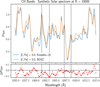 |
Fig. 1 Synthetic solar spectrum in the CH band region around ~4300 Å at the X-shooter resolution (R = 10 000) from the two employed reference grids: the grid computed by Knowles et al. (2021, blue), and the updated BOSZ library (orange). The selected CH bands (see Table 1), where the [C/Fe] abundance is measured, are delimited by the dashed vertical black lines. The flux difference at each wavelength between the two synthetic solar spectra is shown in the bottom panel. |
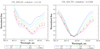 |
Fig. 2 Example of the fit carried out by the spectrum synthesis code GAUGUIN for the two CH analysed bands (showed in Table 1) in the solar reflected spectrum of asteroid Vesta, observed by the spectrograph HARPS (Mayor et al. 2003). It was convolved to the X-shooter spectral resolution (R = 10 000). The normalised observed spectrum is shown with open red diamonds, and the solution is indicated by blue crosses. The reference synthetic spectrum grid (from Knowles et al. 2021) is colour-coded according to the [C/Fe] abundance value. |
Abundance uncertainty associated with the stellar atmosphere parameters.
3.3 Selection of the best analysed X-shooter sample
Based on the CH band selection shown in Table 1, we only analysed the observed X-shooter spectra from the UVB arm (300–556 nm) in order to be able to derive the [C/Fe] stellar abundances. It consists of an original sample of 598 UVB spectra that corresponds to 504 stars.
We followed the same criteria as described by Santos-Peral et al. (2023) for the selection of the final XSL working sample (see Sect. 3.4 therein). In brief, we only kept the observed spectra with S/N > 20 pixel–1 (we discarded ~30 UVB spectra). Additionally, according to the error in the XSL parameter estimates at lower temperatures (Arentsen et al. 2019) and the lack of valid synthetic spectra at Teff > 6500 K because of sensitivity problems in the line-broadening caused by stellar rotation and macroturbulence, we only kept stars with 4000 ≤ Teff ≤ 6500 K to minimise inaccurate abundance values in the final catalogue. Moreover, none of the previously identified XSL carbon stars by Gonneau et al. (2016) are part of the stellar abundance sample we studied.
4 Derived [C/Fe] abundances from the CH band
For each individual X-shooter spectrum, the algorithm GAUGUIN yields separate [C/Fe] abundance measurements corresponding to each CH band listed in Table 1. To derive the final [C/Fe] abundance for each star along with its associated internal uncertainties, we followed the method and quality criteria outlined by Santos-Peral et al. (2023). This approach accounts for the two independent abundance estimates obtained per spectrum (one for each CH band) and for cases when multiple spectra were available for the same star.
In this regard, we estimated the sensitivity of the derived [C/Fe] abundances to the uncertainties on the input XSL stellar atmospheric parameters (Teff, log(g), and [Fe/H]). As followed by Santos-Peral et al. (2023), we performed multiple Monte Carlo realisations of the atmospheric parameters associated with the input spectra. Table 2 illustrates the measured dispersion for different stellar types and metallicity regimes when each synthetic grid was used separately. We adopted these dispersions as estimators of the uncertainties. The reported [C/Fe] abundance uncertainties are generally small, lower than ~0.1 dex, and the precision is similar for the two reference grids we adopted.
We first performed an exhaustive analysis with the computed theoretical spectral library by Knowles et al. (2021), which we later complemented by the comparison with the more recent and updated BOSZ synthetic stellar spectral library (Mészáros et al. 2024). Beforehand, we confirmed the accuracy of each synthetic grid we used by deriving the [Mg/Fe] abundances from the X-shooter catalogue and comparing them to the well-validated measurements from Santos-Peral et al. (2023). This is illustrated in Appendix B.
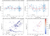 |
Fig. 3 Top row: stellar abundance ratios [C/Fe] vs. [Fe/H] of the X-shooter catalogue after applying the optimal method, with the original synthetic grid from Knowles et al. (2021) (top left) and with the extended [C/Fe] dimension (top right), with the estimated internal uncertainties as vertical error bars. Each red point and error bar corresponds to the measured [C/Fe] average and scatter in metallicity bins of 0.5 dex. Bottom row: HR diagrams of the final X-shooter stellar sample with reliable [C/Fe] abundance measurements from the extended grid over the whole analysed X-shooter sample in this work (grey crosses, bottom left), and colour-coded by the carbon abundance estimate (grey crosses, bottom right). |
4.1 Results based on sMILES (Knowles et al. 2021)
Figure 3 shows the measured [C/Fe] abundances as a function of the stellar metallicity [Fe/H] for the best-analysed XSL sample, together with their estimated internal uncertainties, using the grid from Knowles et al. (2021, described in Sect. 3.1.1) before (top left panel) and after extending the [C/Fe] dimension (top right panel). For both cases, the [C/Fe] abundances clearly describe a dispersed (σ[C/Fe] ~ 0.2–0.3 dex) flat trend around [C/Fe] ~ 0.0 dex throughout the covered metallicity range (–2.5 < [Fe/H] < +0.5 dex). As mentioned in Sect. 3.2, previous works that analysed the CH molecular bands reported a flat trend with respect to metallicity (a complete comparison with the literature is discussed in Sect. 4.3). The main remarkable feature is the observed convex curve at low [C/Fe] abundances around [Fe/H] ~ –0.5 dex, which seems to be present in some previous observational studies as well (e.g. APOGEE DR16, Jönsson et al. 2020). With this analysis, we emphasise the importance of the grid dimension in the abundance space ([C/Fe]i) because it clearly delimits the range of [C/Fe] estimates, which are larger and dispersed when we applied the extended synthetic grid, and also changes the stellar sample with high-quality [C/Fe] measurements (from 199 to 176 stars). For the last case, we also highlight that only stars with [C/Fe] > 0.0 dex in the very metal-poor regime ([Fe/H] ≤ –2.0 dex) are present.
The covered parameters in the HR diagram for the final sample (using the extended grid) are also illustrated in Fig. (bottom row). We measured carbon abundances for different stellar types (67% of the sample are giants) that are well distributed in the parameter space (4000 ≲ Teff ≲ 6000 K; –2.5 ≲ [Fe/H] ≲ +0.5 dex). Tentatively, the completeness of this sample in the atmospheric parameter and chemical space motivates the inclusion of carbon enhancements in evolutionary stellar population synthesis models.
Additionally, it is worth noting that we do not observe any trend with the effective temperature or the surface gravity of the stars. Figure 4 shows a flat and dispersed trend of the derived carbon abundances from each individual CH band with respect to these atmospheric parameters. It is noteworthy that the reported convex curve at low [C/Fe] in Fig. 3 is not visible in these diagrams. This feature is thus specific to the stellar metallicity. The unbiased parameter-dependence of the [C/Fe] abundance estimate constitutes a strong baseline for our research to provide a complete [C/Fe] abundance catalogue.
Furthermore, we evaluated possible abundance internal biases in our method by comparing the individual [C/Fe] estimates from each CH band for the cases where they are both well measured (151 stars). Figure 5 shows the direct [C/Fe] band-to-band abundance comparison between the two spectral regions, colour-coded with the effective stellar temperature, surface gravity, and metallicity. The agreement between the independent abundance estimates from each CH band is good in general. It almost reproduces a perfect linear relation with identical [C/Fe] values (average offset of ~0.01 dex). This compatibility supports the robustness of the implemented method in deriving [C/Fe] abundances from individual CH molecular bands.
The fits in the two CH regions for hot dwarf stars (Teff > 5000 K) are slightly better. This behaviour was expected because the increased effective temperature reduces the blended and molecular lines in the spectrum, and, according to the literature, the derived carbon abundance in these stars probably does not reflect the initial carbon composition with which the star was born because of the internal mixing in the atmospheres of giant stars (e.g. Gallino et al. 1998; Gratton et al. 2000). Figure 6 illustrates the [C/Fe] abundance ratios relative to the metallicity [Fe/H] for the most reliable stellar cases in the analysed X-shooter sample: those with S/N > 50 (top left panel), hot stars with Teff > 5000 Κ (top right panel), and dwarf stars alone (bottom left panel). Additionally, we show the stars that could have passed through the first dredge-up phase (Teff < 4500 Κ and logg < 3.0 cm s–2, bottom right panel). For each subsample, the reported stellar distribution is very similar with respect to the distribution described in Fig. 3. That is to say, a flat dispersed trend over the whole metallicity range that reproduces a convex curve at low [C/Fe] abundances around [Fe/H] ~ –0.5 dex, and we only find stars with [C/Fe] > 0.0 dex in the very metal-poor regime.
The unbiased general trend shown in Fig. 6, regardless of the selected stellar type or spectrum signal-to-noise ratio, does not allow us to distinguish any individual star in the final XSL sample as having a high-quality [C/Fe] abundance estimate. However, it is encouraging that we appear to be able to derive carbon abundances for both dwarfs and giants without distinction.
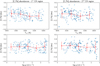 |
Fig. 4 Derived [C/Fe] abundance ratio from each analysed CH band separately (left and right columns, shown in Table 1 ) as a function of the stellar effective temperature (top row) and surface gravity (bottom row). Each red point and error bar corresponds to the measured average and scatter in temperature and gravity bins of 500 Κ and log 1 cm s–2, respectively. |
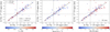 |
Fig. 5 Comparison between the derived [C/Fe] abundances from the individual analysed CH bands, colour-coded according to the effective temperature (left), surface gravity (middle), and metallicity (right) of the star. The dashed black line reproduces the 1:1 relation. The mean (μ), standard deviation (σ), median, and robust standard deviation (i.e. ~1.48 times the median absolute deviation, MAD) of the offsets are indicated in the first panel. |
4.2 Results based on BOSZ (Mészáros et al. 2024)
Secondly, we implemented the updated BOSZ synthetic spectral library (described in detail in Sect. 3.1.2) in GAUGUIN as the new reference synthetic grid to derive the [C/Fe] abundances. We analysed the same CH molecular bands (Table 1) over the same selected XSL stellar sample illustrated before in order to compare the results with those previously determined with the computed synthetic grid by Knowles et al. (2021).
Figure 7 illustrates the resulting fit for the observed solar spectrum at the X-shooter resolution (see also for Arcturus in Appendix A). Similarly, as shown in previous Fig. 2, the fit is good and the correlation of the [C/Fe] abundance in the CH bands is smooth. The average [C/Fe] abundance of [C/Fe] ≈ –0.52 dex is significantly different from that estimated with the Knowles et al. (2021) grid (![Mathematical equation: $\overline {\left[ {{\rm{C}}/{\rm{Fe}}} \right]} \approx + 0.12$](/articles/aa/full_html/2025/09/aa55668-25/aa55668-25-eq2.png) dex), however, and shows an averaged difference of |Δ[C/Fe]| ≈ 0.64 dex. This substantial disagreement might be explained by the differences in the lines profiles between the synthetic grids in the CH region (shown in Fig. 1) that may affect the [C/Fe] estimate procedure, although both grids were fully consistent in the [Mg/Fe] estimates (see Appendix B).
dex), however, and shows an averaged difference of |Δ[C/Fe]| ≈ 0.64 dex. This substantial disagreement might be explained by the differences in the lines profiles between the synthetic grids in the CH region (shown in Fig. 1) that may affect the [C/Fe] estimate procedure, although both grids were fully consistent in the [Mg/Fe] estimates (see Appendix B).
In addition, we re-evaluated the comparison between the derived [C/Fe] abundances from each CH band. Figure 8 also shows a good agreement (average offset of ~0.03 dex), that is, a strong compatibility. This indicates that the applied method remains robust in deriving [C/Fe] abundances from the CH molecular bands, as discussed in Fig. 5 for the grid from Knowles et al. (2021). No trend with the stellar atmospheric parameters (i.e. Teff, log g) is visible either, and the final abundance sample is equally well distributed in the HR diagram parameter coverage.
Figure 9 shows the obtained [C/Fe] abundance ratio versus the metallicity [Fe/H] for the XSL sample (left panel), using the updated BOSZ synthetic spectral library (Mészáros et al. 2024). We observe a similar, but more dispersed (σ[C/Fe] ~ 0.4 dex), evolution of [C/Fe] to that depicted in Fig. 3 with the Knowles et al. (2021) grid. This behaviour was also found when we applied the same quality selections explained in Fig. 6. In addition, we directly compared the [C/Fe] abundance results from each adopted reference synthetic grid (middle panel). The X-shooter stars are randomly distributed in a wide [C/Fe] abundance range (–0.4 dex ≲ [C/Fe] ≲ +0.4 dex) and show significant differences in absolute terms up to |Δ[C/Fe]| ~ 0.8 dex, which implies a strong model dependence in the abundance estimate. Lastly, we also studied these differences as a function of the carbon estimates from Knowles et al. (2021) (right panel). The trend decreases with [Fe/H], where most of the stars with low measured [C/Fe] abundances (e.g. [C/Fe] < –0.2 dex) with the Knowles et al. (2021) grid present the highest [C/Fe] values when the BOSZ grid from Mészáros et al. (2024) is implemented. Surprisingly, although the overall [C/Fe] versus [Fe/H] distribution looks similar, the individual stellar compositions vary strongly with the synthetic grid.
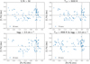 |
Fig. 6 [C/Fe] vs. [Fe/H] with the extended synthetic grid from Knowles et al. (2021). We show only the cases with high signal-to-noise (S/N > 50, top left), hot stars (Teff > 5000 K, top right), dwarfs (log(g) > 3.5 cm s–2, bottom left), and cool giant stars (Teff < 4500 Κ and log(g) < 3.0 cm s–2, bottom right). |
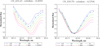 |
Fig. 7 Same as Fig. 2, but using the BOSZ synthetic spectrum grid (Mészáros et al. 2024) as a reference. |
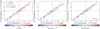 |
Fig. 8 Same as Fig. 5, but using the BOSZ spectral library for deriving the [C/Fe] stellar abundances. |
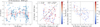 |
Fig. 9 Left: obtained abundance ratios [C/Fe] vs. [Fe/H] of the X-shooter catalogue with the BOSZ synthetic spectrum grid (Mészáros et al. 2024). The red points are defined as in Fig. 3. Middle: direct comparison between the derived [C/Fe] abundances with each reference synthetic grid, colour-coded according to the stellar metallicity. The dashed black line and the offset estimates are the same as described in Fig. 5. Right: difference in the measured [C/Fe] abundance between the grids, colour-coded by the effective temperature, as a function of the [C/Fe] estimate previously determined with the grid from Knowles et al. (2021). |
4.3 Comparison with literature studies
On the basis of the previous analysis, we were not able to determine which set of stellar X-shooter [C/Fe] abundances was more accurate in accordance with an objective criterion. For this reason, we revised carbon literature studies in detail in order to draw more reliable conclusions.
Figure 10 shows the [C/Fe] abundance versus metallicity [Fe/H] plane from a wide variety of published stellar catalogues in the literature. The study results are heterogeneous, even for those that analysed the same carbon lines. As mentioned before, these works only selected dwarf stars in their samples in order to avoid the potentially misleading carbon measurements from the giants and AGB atmospheres. Regardless of the applied method, every work shows a large star-to-star dispersion in [C/Fe] at a fixed metallicity, which agrees with what we observed in our study. In particular, the works that analysed atomic CI lines show a decrease of [C/Fe] with metallicity, similar to that observed for the α-elements evolution. Moreover, we highlight the presence of a similar [C/Fe] convex shape around [Fe/H] ~ –0.5 dex in Nissen et al. (2014) for the well-known CI lines (5052.16, 5380.34 Å), which has also been illustrated by the APOGEE DR16 data (see Fig. 12 in Jönsson et al. 2020). This feature, although slightly more diffuse, seems to be present in Suárez-Andrés et al. (2017) for the CH 4300 Å region as well, which shows a flatter carbon trend as a function of [Fe/H].
Complementary, in Fig. 11 we directly compared our [C/Fe] abundance results (from the two synthetic grids separately) for a subsample of stars in common with the literature (APOGEE DR17, Abdurro’uf et al. 2022). We previously verified the compatibility of the stellar parameters (Teff, log(g), [Fe/H]) among the different catalogues in order to be consistent. The agreement was excellent, with no biases and almost identical values. For the carbon abundances, Fig. 11 shows a very dispersed relation with respect to the literature, however, that is comparable for the two reference grids we adopted. It presents a similar median and σMAD estimates around –0.1 and 0.24 dex, respectively. Once again, the very close resemblance between the quality and accuracy of the different measured [C/Fe] abundances with the two employed synthetic spectral libraries prevents us from determining which would be more suitable for the carbon characterisation of the X-shooter spectral library.
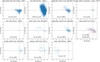 |
Fig. 10 [C/Fe] vs. [Fe/H] abundance ratios of literature studies with different carbon line selections, as indicated at the top. |
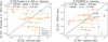 |
Fig. 11 Direct comparison between the derived stellar abundance ratio [C/Fe] in this work, using the synthetic grid from Knowles et al. (2021) (left) and the BOSZ library (Mészáros et al. 2024, right), and the abundance estimate for stars in common with the literature, with their respective reported uncertainties as error bars. The dashed black line is the same as in Fig. 5. |
4.4 Reported caveats
To summarise, the two 5D synthetic spectral libraries we employed enable a precise [C/Fe] abundance determination from CH molecular bands. The effect of the hydrogen atom seems to be negligible since [C/Fe] variations can be reproduced and measured at a given [Fe/H]. Every quality test satisfactorily indicated that we achieved a large unbiased [C/Fe] abundance catalogue, such as the quality of the line profile fit to derive the abundances (Figs. 2 and 7), the compatibility of the measured values between the bands we analysed (Figs. 5 and 8), or the lack of a parameter dependence in the carbon estimate (Fig. 4). In principle, these catalogues seem ideal to shed new light on the carbon analysis problems and to improve stellar population models in the near future.
Nevertheless, we measured different and unpredictable [C/Fe] abundance results for the same star (up to |Δ[C/Fe]| ~ 0.8 dex) without an apparent reason by just varying the reference synthetic grid (with equal [C/Fe] dimension) in the spectrum synthesis algorithm. They are well-proven theoretical grids that did not show different abundance estimates like this for other chemical species (e.g. [Mg/Fe]; see Appendix B) with the same method. This means that the predominant model dependence in the [C/Fe] abundance measurements might arise from some hidden issues in the carbon modelling of the crowded and blended CH 4300 Å spectral region. Small differences in the synthetic models may induce a large disparity in the abundance estimate procedure (e.g. observed spectrum normalisation or line fit), leading to completely disparate results.
Complementarily, the medium spectral resolution of the X-shooter spectrograph (R ~ 10 000) might not be high enough for properly measuring carbon abundances. A high spectral resolution (R ≳ 50 000) generally allows us to disentangle blended lines and define a reliable continuum (Nissen & Gustafsson 2018). On this basis, we analysed the typically studied unblended CI lines in the literature (5052.16, 5380.34 Å) for the solar spectrum at R = 110 000 (same resolution as Suárez-Andrés et al. 2017, who also analysed the CH regions). Figure 12 illustrates the fit we obtained for each line separately. These atomic lines are weaker that the CH 4300 Å bands, which also vary smoothly with the [C/Fe] abundance. We measured compatible abundance values from each CI line, ![Mathematical equation: $\overline {\left[ {{\rm{C}}/{\rm{Fe}}} \right]} \approx + 0.14$](/articles/aa/full_html/2025/09/aa55668-25/aa55668-25-eq3.png) dex, which is similar to the value obtained at the X-shooter resolution from the CH regions (
dex, which is similar to the value obtained at the X-shooter resolution from the CH regions (![Mathematical equation: $\overline {\left[ {{\rm{C}}/{\rm{Fe}}} \right]} \approx + 0.12$](/articles/aa/full_html/2025/09/aa55668-25/aa55668-25-eq4.png) dex, see Fig. 2). This compatibility of the derived [C/Fe] abundances for the solar spectrum with different resolutions and from different carbon lines supports the robustness of the implemented synthetic spectrum algorithm in deriving [C/Fe] abundances. Consequently, the reported inconsistencies in our results might come from intrinsic issues in the carbon element modelling of the theoretical synthetic spectra.
dex, see Fig. 2). This compatibility of the derived [C/Fe] abundances for the solar spectrum with different resolutions and from different carbon lines supports the robustness of the implemented synthetic spectrum algorithm in deriving [C/Fe] abundances. Consequently, the reported inconsistencies in our results might come from intrinsic issues in the carbon element modelling of the theoretical synthetic spectra.
With this analysis, we would like to note the potential error sources associated with the use of spectrum synthesis codes to derive stellar carbon abundances, which may lead to possible misunderstandings in the measured results for any stellar type.
5 Conclusions
We carried out a detailed spectroscopic analysis of the carbon abundance determination for the X-shooter Spectral Library (XSL), a large empirical stellar catalogue that is used as a benchmark for the development of stellar population models. We used the stellar sample selected by Santos-Peral et al. (2023) for the previous α-element (Mg, Ca) characterisation of the XSL, following the same abundance quality criteria.
We implemented the spectrum synthesis code GAUGUIN for deriving [C/Fe] abundances from individual CH molecular bands around the 4300 Å spectral region because unblended atomic CI lines cannot be resolved at the XSL resolution (R ~ 10 000). The effect of the hydrogen atom seems to be negligible because the [C/Fe] differences can be properly reproduced and measured from these bands at a given [Fe/H]. In order to evaluate the accuracy and the model dependence of the measured [C/Fe] abundances, we used two different computed sets of 5D (Teff, log(g), [M/H], [α/Fe], and [C/Fe]) reference synthetic spectrum grids: a theoretical library used for the computation of the semi-empirical MILES stellar spectra (sMILES; Knowles et al. 2021), and the updated BOSZ synthetic stellar spectral library (Mészáros et al. 2024). We previously checked that they were fully consistent in their accurate [Mg/Fe] abundance estimates.
From each adopted reference theoretical grid, we obtained a precise XSL [C/Fe] abundance catalogue of around 200 stars with an excellent parameter coverage that showed no biases with the effective temperature or the surface gravity of the stars. Satisfactorily, we derived carbon abundances for both dwarfs and giants, with a similar high-quality [C/Fe] abundance estimate. In addition, the agreement between the individual [C/Fe] abundance measurements from each analysed CH band was also remarkable (with an average difference always lower than 0.03 dex), regardless of the adopted synthetic grid. Moreover, we measured compatible [C/Fe] solar abundance values from different spectral resolutions and atomic carbon lines, which supports the hypothesis that the implemented method is reliable, although a calibration is needed to reproduce the solar composition. The final derived stellar abundance ratio [C/Fe] relative to the metallicity [Fe/H] always presented a flat behaviour, dispersed (σ[C/Fe] ~ 0.2–0.4 dex) around the zero [C/Fe] value for the whole metallicity range we covered (–2.5 < [Fe/H] < +0.5 dex). We observed no decreasing trend of [C/Fe] with metallicity, as suggested in the literature.
We were able to provide a complete and unbiased [C/Fe] abundance catalogue with a well-tested robust method. This may constitute an important baseline research for including carbon-enhancements in the development of evolutionary stellar population synthesis models. Nevertheless, we measured different, disparate, and unpredictable [C/Fe] abundance values for the same analysed star (differences up to |Δ[C/Fe]| ~ 0.8 dex) for the different reference synthetic grids in the spectrum synthesis algorithm. Consequently, there is a predominant model dependence in the [C/Fe] abundance measurements from the crowded and blended CH 4300 Å region.
With the use of a spectral synthesis code to derive stellar carbon abundances in the CH 4300 Å band, we therefore found that potential sources oferror might be associated with unknown intrinsic constraints inside the carbon modelling of the theoretic synthetic spectra. This leads to inaccurate [C/Fe] abundance estimates for any stellar type, but does not significantly affect the measured high-quality precision.
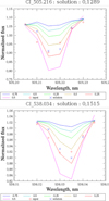 |
Fig. 12 Same as Fig. 2, but for the most frequently used CI lines in the literature (5052.16, 5380.34 Å) in the observed solar spectrum at R = 110 000. The reference synthetic spectrum grid is taken from Knowles et al. (2021). |
Acknowledgements
We thank the referee for his/her suggestions and discussions. The authors thank A. Recio-Blanco, P. de Laverny, C. Ordenovic and M. A. Álvarez for having developed the GAUGUIN method within the Gaia/GSP-spec context and having shared it with us. For any questions related to this algorithm, please contact directly A. Recio-Blanco and P. de Laverny. P.S.P. and P.S.B acknowledges financial support by the Spanish Ministry of Science and Innovation through the research grant PID2019-107427GB-C31 and PID2022-138855NB-C3. P.S.P. also acknowledges financial support by the European Union – NextGenerationEU under a Margarita Salas contract. A.V. acknowledges support from grants PID2021-123313NA-I00 and PID2022-140869NB-I00 from the Spanish Ministry of Science and Innovation. This work has also been supported through the IAC project TRACES, which is partially supported through the state budget and the regional budget of the Consejería de Economía, Industria, Comercio y Conocimiento of the Canary Islands Autonomous Community. This work has made use of data from the European Space Agency (ESA) mission Gaia (https://www.cosmos.esa.int/gaia), processed by the Gaia Data Processing and Analysis Consortium (DPAC, https://www.cosmos.esa.int/web/gaia/dpac/consortium). Funding for the DPAC has been provided by national institutions, in particular the institutions participating in the Gaia Multilateral Agreement. Most of the calculations have been performed with the high-performance computing facility SIGAMM, hosted by the Observatorie de la Côte d’Azur (OCA).
References
- Abdurro’uf, Accetta, K., Aerts, C., et al. 2022, ApJS, 259, 35 [NASA ADS] [CrossRef] [Google Scholar]
- Ahumada, R., Allende Prieto, C., Almeida, A., et al. 2020, ApJS, 249, 3 [NASA ADS] [CrossRef] [Google Scholar]
- Alexeeva, S. A., & Mashonkina, L. I. 2015, MNRAS, 453, 1619 [NASA ADS] [CrossRef] [Google Scholar]
- Allende Prieto, C., Koesterke, L., Hubeny, I., et al. 2018, A&A, 618, A25 [NASA ADS] [CrossRef] [EDP Sciences] [Google Scholar]
- Amarsi, A. M., Nissen, P. E., & Skúladóttir, Á. 2019, A&A, 630, A104 [NASA ADS] [CrossRef] [EDP Sciences] [Google Scholar]
- Andersson, H., & Edvardsson, B. 1994, A&A, 290, 590 [NASA ADS] [Google Scholar]
- Ardern-Arentsen, A., Kane, S. G., Belokurov, V., et al. 2025, MNRAS, 537, 1984 [Google Scholar]
- Arentsen, A., Prugniel, P., Gonneau, A., et al. 2019, A&A, 627, A138 [NASA ADS] [CrossRef] [EDP Sciences] [Google Scholar]
- Asplund, M., Grevesse, N., Sauval, A. J., Allende Prieto, C., & Blomme, R. 2005, A&A, 431, 693 [NASA ADS] [CrossRef] [EDP Sciences] [Google Scholar]
- Baldwin, C., McDermid, R. M., Kuntschner, H., Maraston, C., & Conroy, C. 2018, MNRAS, 473, 4698 [Google Scholar]
- Bensby, T., & Feltzing, S. 2006, MNRAS, 367, 1181 [CrossRef] [Google Scholar]
- Bensby, T., Gould, A., Asplund, M., et al. 2021, A&A, 655, A117 [NASA ADS] [CrossRef] [EDP Sciences] [Google Scholar]
- Beverage, A. G., Slob, M., Kriek, M., et al. 2025, ApJ, 979, 249 [Google Scholar]
- Bijaoui, A., Recio-Blanco, A., de Laverny, P., & Ordenovic, C. 2012, Statist. Methodol., 9, 55 [Google Scholar]
- Bruzual, G., & Charlot, S. 2003, MNRAS, 344, 1000 [NASA ADS] [CrossRef] [Google Scholar]
- Carbon, D. F., Barbuy, B., Kraft, R. P., Friel, E. D., & Suntzeff, N. B. 1987, PASP, 99, 335 [NASA ADS] [CrossRef] [Google Scholar]
- Carrasco, E., Mollá, M., García-Vargas, M. L., et al. 2021, MNRAS, 501, 3568 [CrossRef] [Google Scholar]
- Cervantes, J. L., Coelho, P., Barbuy, B., & Vazdekis, A. 2007, in IAU Symposium, 241, Stellar Populations as Building Blocks of Galaxies, eds. A. Vazdekis & R. Peletier, 167 [Google Scholar]
- Chen, Y.-P., Trager, S. C., Peletier, R. F., et al. 2014, A&A, 565, A117 [NASA ADS] [CrossRef] [EDP Sciences] [Google Scholar]
- Conroy, C., & van Dokkum, P. G. 2012, ApJ, 760, 71 [Google Scholar]
- Conroy, C., Villaume, A., van Dokkum, P. G., & Lind, K. 2018, ApJ, 854, 139 [Google Scholar]
- Creevey, O. L., Sordo, R., Pailler, F., et al. 2023, A&A, 674, A26 [NASA ADS] [CrossRef] [EDP Sciences] [Google Scholar]
- Cristallo, S., Piersanti, L., Straniero, O., et al. 2011, ApJS, 197, 17 [NASA ADS] [CrossRef] [Google Scholar]
- Dahmer-Hahn, L. G., Riffel, R., Rodríguez-Ardila, A., et al. 2018, MNRAS, 476, 4459 [Google Scholar]
- de La Rosa, I. G., La Barbera, F., Ferreras, I., & de Carvalho, R. R. 2011, MNRAS, 418, L74 [NASA ADS] [CrossRef] [Google Scholar]
- de Laverny, P., Recio-Blanco, A., Worley, C. C., & Plez, B. 2012, A&A, 544, A126 [NASA ADS] [CrossRef] [EDP Sciences] [Google Scholar]
- Delgado Mena, E., Israelian, G., González Hernández, J. I., et al. 2010, ApJ, 725, 2349 [NASA ADS] [CrossRef] [Google Scholar]
- Ecuvillon, A., Israelian, G., Santos, N. C., et al. 2004, A&A, 426, 619 [NASA ADS] [CrossRef] [EDP Sciences] [Google Scholar]
- Delgado Mena, E., Adibekyan, V., Santos, N. C., et al. 2021, A&A, 655, A99 [NASA ADS] [CrossRef] [EDP Sciences] [Google Scholar]
- Eftekhari, E., La Barbera, F., Vazdekis, A., Allende Prieto, C., & Knowles, A. T. 2022, MNRAS, 512, 378 [NASA ADS] [CrossRef] [Google Scholar]
- Eftekhari, E., Vazdekis, A., Riffel, R., et al. 2025, A&A, 693, A238 [NASA ADS] [CrossRef] [EDP Sciences] [Google Scholar]
- Fernández-Alvar, E., Carigi, L., Schuster, W. J., et al. 2018, ApJ, 852, 50 [CrossRef] [Google Scholar]
- Franchini, M., Morossi, C., Di Marcantonio, P., et al. 2020, ApJ, 888, 55 [NASA ADS] [CrossRef] [Google Scholar]
- Frebel, A., Johnson, J. L., & Bromm, V. 2007, MNRAS, 380, L40 [NASA ADS] [CrossRef] [Google Scholar]
- Freeman, K., & Bland-Hawthorn, J. 2002, ARA&A, 40, 487 [Google Scholar]
- Gallino, R., Arlandini, C., Busso, M., et al. 1998, ApJ, 497, 388 [Google Scholar]
- Gonneau, A., Lançon, A., Trager, S. C., et al. 2016, A&A, 589, A36 [NASA ADS] [CrossRef] [EDP Sciences] [Google Scholar]
- Gonneau, A., Lyubenova, M., Lançon, A., et al. 2020, A&A, 634, A133 [NASA ADS] [CrossRef] [EDP Sciences] [Google Scholar]
- Gratton, R. G., Sneden, C., Carretta, E., & Bragaglia, A. 2000, A&A, 354, 169 [NASA ADS] [Google Scholar]
- Grevesse, N., Asplund, M., & Sauval, A. J. 2007, Space Sci. Rev., 130, 105 [Google Scholar]
- Guiglion, G., de Laverny, P., Recio-Blanco, A., et al. 2016, A&A, 595, A18 [NASA ADS] [CrossRef] [EDP Sciences] [Google Scholar]
- Gustafsson, B., Karlsson, T., Olsson, E., Edvardsson, B., & Ryde, N. 1999, A&A, 342, 426 [NASA ADS] [Google Scholar]
- Gustafsson, B., Edvardsson, B., Eriksson, K., et al. 2008, A&A, 486, 951 [NASA ADS] [CrossRef] [EDP Sciences] [Google Scholar]
- Harris, J., & Zaritsky, D. 2009, AJ, 138, 1243 [NASA ADS] [CrossRef] [Google Scholar]
- Hinkle, K., Wallace, L., Valenti, J., & Harmer, D. 2000, Visible and Near Infrared Atlas of the Arcturus Spectrum 3727–9300 Å [Google Scholar]
- Hubeny, I., & Lanz, T. 2017, arXiv e-prints [arXiv: 1706.01859] [Google Scholar]
- Hubeny, I., & Lanz, T. 2000, in American Astronomical Society Meeting Abstracts, 197, American Astronomical Society Meeting Abstracts, 78.12 [Google Scholar]
- Hubeny, I., Allende Prieto, C., Osorio, Y., & Lanz, T. 2021, arXiv e-prints [arXiv:2104.02829] [Google Scholar]
- Iben, Jr., I. 1965, ApJ, 142, 1447 [NASA ADS] [CrossRef] [Google Scholar]
- Jönsson, H., Holtzman, J. A., Allende Prieto, C., et al. 2020, AJ, 160, 120 [Google Scholar]
- Karakas, A. I., & Lattanzio, J. C. 2014, PASA, 31, e030 [NASA ADS] [CrossRef] [Google Scholar]
- Knowles, A. T., Sansom, A. E., Coelho, P. R. T., et al. 2019, MNRAS, 486, 1814 [NASA ADS] [CrossRef] [Google Scholar]
- Knowles, A. T., Sansom, A. E., Allende Prieto, C., & Vazdekis, A. 2021, MNRAS, 504, 2286 [NASA ADS] [CrossRef] [Google Scholar]
- Knowles, A. T., Sansom, A. E., Vazdekis, A., & Allende Prieto, C. 2023, MNRAS, 523, 3450 [NASA ADS] [CrossRef] [Google Scholar]
- Kobayashi, C., Karakas, A. I., & Lugaro, M. 2020, ApJ, 900, 179 [Google Scholar]
- Koesterke, L. 2009, in American Institute of Physics Conference Series, 1171, Recent Directions in Astrophysical Quantitative Spectroscopy and Radiation Hydrodynamics, eds. I. Hubeny, J. M. Stone, K. MacGregor, & K. Werner (AIP), 73 [NASA ADS] [Google Scholar]
- Kurucz, R. L. 1979, ApJS, 40, 1 [NASA ADS] [CrossRef] [Google Scholar]
- Kurucz, R. 1993, Robert Kurucz CD-ROM, 13 [Google Scholar]
- La Barbera, F., Vazdekis, A., Ferreras, I., et al. 2016, MNRAS, 457, 1468 [Google Scholar]
- Le Borgne, D., Rocca-Volmerange, B., Prugniel, P., et al. 2004, A&A, 425, 881 [CrossRef] [EDP Sciences] [Google Scholar]
- Lebzelter, T., Mowlavi, N., Marigo, P., et al. 2018, A&A, 616, L13 [NASA ADS] [CrossRef] [EDP Sciences] [Google Scholar]
- Maraston, C., & Strömbäck, G. 2011, MNRAS, 418, 2785 [Google Scholar]
- Masseron, T., Plez, B., Van Eck, S., et al. 2014, A&A, 571, A47 [NASA ADS] [CrossRef] [EDP Sciences] [Google Scholar]
- Maraston, C., Hill, L., Thomas, D., et al. 2020, MNRAS, 496, 2962 [Google Scholar]
- Mayor, M., Pepe, F., Queloz, D., et al. 2003, The Messenger, 114, 20 [NASA ADS] [Google Scholar]
- Mészáros, S., Allende Prieto, C., Edvardsson, B., et al. 2012, AJ, 144, 120 [Google Scholar]
- Mészáros, S., Bohlin, R., Allende Prieto, C., et al. 2024, A&A, 688, A197 [NASA ADS] [CrossRef] [EDP Sciences] [Google Scholar]
- Mollá, M., García-Vargas, M. L., & Bressan, A. 2009, MNRAS, 398, 451 [CrossRef] [Google Scholar]
- Nissen, P. E., & Gustafsson, B. 2018, A&A Rev., 26, 6 [NASA ADS] [CrossRef] [Google Scholar]
- Nissen, P. E., Chen, Y. Q., Carigi, L., Schuster, W. J., & Zhao, G. 2014, A&A, 568, A25 [NASA ADS] [CrossRef] [EDP Sciences] [Google Scholar]
- Osborn, Z., Karakas, A., Kemp, A., et al. 2025, PASA, 42, e020 [Google Scholar]
- Pavlenko, Y. V., Kaminsky, B. M., Jenkins, J. S., et al. 2019, A&A, 621, A112 [NASA ADS] [CrossRef] [EDP Sciences] [Google Scholar]
- Prugniel, P., & Soubiran, C. 2001, A&A, 369, 1048 [CrossRef] [EDP Sciences] [Google Scholar]
- Ramírez, I., & Allende Prieto, C. 2011, ApJ, 743, 135 [Google Scholar]
- Recio-Blanco, A., de Laverny, P., Kordopatis, G., et al. 2014, A&A, 567, A5 [NASA ADS] [CrossRef] [EDP Sciences] [Google Scholar]
- Recio-Blanco, A., de Laverny, P., Allende Prieto, C., et al. 2016, A&A, 585, A93 [NASA ADS] [CrossRef] [EDP Sciences] [Google Scholar]
- Recio-Blanco, A., de Laverny, P., Palicio, P. A., et al. 2023, A&A, 674, A29 [NASA ADS] [CrossRef] [EDP Sciences] [Google Scholar]
- Sánchez-Blázquez, P., Peletier, R. F., Jiménez-Vicente, J., et al. 2006, MNRAS, 371, 703 [Google Scholar]
- Santos-Peral, P., Recio-Blanco, A., de Laverny, P., Fernández-Alvar, E., & Ordenovic, C. 2020, A&A, 639, A140 [NASA ADS] [CrossRef] [EDP Sciences] [Google Scholar]
- Santos-Peral, P., Sánchez-Blázquez, P., Vazdekis, A., & Palicio, P. A. 2023, A&A, 672, A166 [NASA ADS] [CrossRef] [EDP Sciences] [Google Scholar]
- Sestito, F., Ardern-Arentsen, A., Vitali, S., et al. 2024, A&A, 690, A333 [NASA ADS] [CrossRef] [EDP Sciences] [Google Scholar]
- Suárez-Andrés, L., Israelian, G., González Hernández, J. I., et al. 2017, A&A, 599, A96 [NASA ADS] [CrossRef] [EDP Sciences] [Google Scholar]
- Unni, A., Narang, M., Sivarani, T., et al. 2022, AJ, 164, 181 [NASA ADS] [CrossRef] [Google Scholar]
- Vazdekis, A. 1999, ApJ, 513, 224 [NASA ADS] [CrossRef] [Google Scholar]
- Vazdekis, A., Sánchez-Blázquez, P., Falcón-Barroso, J., et al. 2010, MNRAS, 404, 1639 [NASA ADS] [Google Scholar]
- Vazdekis, A., Coelho, P., Cassisi, S., et al. 2015, MNRAS, 449, 1177 [Google Scholar]
- Vazdekis, A., Koleva, M., Ricciardelli, E., Röck, B., & Falcón-Barroso, J. 2016, MNRAS, 463, 3409 [Google Scholar]
- Vernet, J., Dekker, H., D’Odorico, S., et al. 2011, A&A, 536, A105 [NASA ADS] [CrossRef] [EDP Sciences] [Google Scholar]
- Verro, K., Trager, S. C., Peletier, R. F., et al. 2022a, A&A, 661, A50 [NASA ADS] [CrossRef] [EDP Sciences] [Google Scholar]
- Verro, K., Trager, S. C., Peletier, R. F., et al. 2022b, A&A, 660, A34 [NASA ADS] [CrossRef] [EDP Sciences] [Google Scholar]
- Walcher, C. J., Coelho, P., Gallazzi, A., & Charlot, S. 2009, MNRAS, 398, L44 [NASA ADS] [Google Scholar]
- Zhao, G., Mashonkina, L., Yan, H. L., et al. 2016, ApJ, 833, 225 [Google Scholar]
Appendix A Arcturus
We reproduced the analysis performed for Figs. 2 and 7, considering the spectrum of a cool giant star instead of the solar one. We used Arcturus spectrum provided by Hinkle et al. (2000) as a benchmark, and adopted the atmospheric parameters from Ramírez & Allende Prieto (2011): Teff = 4286 K; log(g) = 1.66 cm s–2; [Fe/H] = –0.52 dex; [C/Fe] = +0.43 ± 0.07 dex.
Figures A.1 and A.2 show the obtained result from the same analysed CH bands (Table 1) with the Knowles et al. (2021) synthetic grid and the BOSZ spectral library (Mészáros et al. 2024), respectively. Similar to the Solar case, we observe a good fit with a remarkable band-to-band abundance agreement from both grids, although different [C/Fe] estimates. We measured ![Mathematical equation: $\overline {\left[ {{\rm{C}}/{\rm{Fe}}} \right]} \approx + 0.28$](/articles/aa/full_html/2025/09/aa55668-25/aa55668-25-eq5.png) dex with Knowles et al. (2021) and
dex with Knowles et al. (2021) and ![Mathematical equation: $\overline {\left[ {{\rm{C}}/{\rm{Fe}}} \right]} \approx + 0.46$](/articles/aa/full_html/2025/09/aa55668-25/aa55668-25-eq6.png) dex with BOSZ, being the latter compatible with the literature value. This leads to an averaged difference of |Δ[C/Fe]| ≈ 0.18 dex between both adopted grids.
dex with BOSZ, being the latter compatible with the literature value. This leads to an averaged difference of |Δ[C/Fe]| ≈ 0.18 dex between both adopted grids.
Therefore, as discussed in the body of the paper, we obtained significant different [C/Fe] estimates depending on the adopted grid, but with a high-quality precision measurement. Unknown intrinsic issues in the carbon modelling may lead to inaccurate stellar carbon abundances.
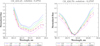 |
Fig. A.1 Same fit as shown in Fig. 2, but for the observed Arcturus spectrum from Hinkle et al. (2000). |
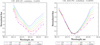 |
Fig. A.2 Same as Fig. A.1, but using the BOSZ synthetic spectrum grid (Mészáros et al. 2024) as a reference. |
Appendix B Preliminary validation analysis: [Mg/Fe] abundance determination
Previously to the carbon abundance analysis, we evaluated the quality and reliability of the used synthetic grids in order to avoid the potential propagation of uncertainties to the stellar abundance measurements. For this purpose, we firstly derived [Mg/Fe] abundances for the same X-shooter abundance catalogue published by Santos-Peral et al. (2023).
As described in detail in Santos-Peral et al. (2020, 2023), the code GAUGUIN interpolates the reference synthetic spectrum grid to the known input stellar parameters (Teff, log(g), [Fe/H], [α/Fe]) of the observed star, generating a new specific-reference grid in the abundance space (e.g. [C/Fe]) to measure the abundance from the analysed spectral region. That is to say, the four input atmospheric parameters of each observed spectrum are fixed and required by GAUGUIN to derive individual chemical abundances. For this reason, it is crucial to verify if we can measure accurate α-element abundances with the employed reference synthetic grids (i.e. Knowles et al. 2021; Mészáros et al. 2024) before extending the analysis to other chemical elements.
Therefore, we analysed the same strong well-known magnesium spectrum lines than in Santos-Peral et al. (2023), who used a completely different synthetic grid implemented for the AMBRE Project (de Laverny et al. 2012) and the Gaia-RYS analysis by the General Stellar Parametriser-spectroscopic (GSP-Spec) module (Recio-Blanco et al. 2023).
Figure B.1 shows the comparison of the derived X-shooter [Mg/Fe] abundances among the three discussed synthetic spectrum grids: the one used by Santos-Peral et al. (2023), and the two implemented here: the computed one by Knowles et al. (2021) and the updated BOSZ library (Mészáros et al. 2024). We only plot stars with chemical abundance measurements that fulfilled the applied quality criteria. We observe a very good agreement between datasets, with small biases for each synthetic grid with respect to Santos-Peral et al. (2023) results: averaged differences less than ~0.005 dex, with most of the stars with almost identical [Mg/Fe] values (bottom-left and bottom-right panels). The abundance estimates between the two grids used in the present work also present a remarkable agreement (![Mathematical equation: $\overline {\left| {\Delta \left[ {{\rm{Mg}}/Fe} \right]} \right|} \~0.02$](/articles/aa/full_html/2025/09/aa55668-25/aa55668-25-eq7.png) dex, see bottom-middle panel)
dex, see bottom-middle panel)
In conclusion, the employed synthetic stellar spectral libraries in this study describe a robust behaviour in their theoretical atmospheric parameters (Teff, log(g), [Fe/H], [α/Fe]), key for an accurate abundance determination.
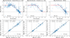 |
Fig. B.1 Comparison between the derived [Mg/Fe] abundances of the X-shooter catalogue (Santos-Peral et al. 2023) and those measured when we used the synthetic grid by Knowles et al. (2021) and the BOSZ library as the reference in the applied methodology. Top row: stellar abundance ratios [Mg/Fe] vs. [Fe/H] from Santos-Peral et al. (2023) (top-left), with the grid by Knowles et al. (2021) (top-middle), and with BOSZ (top-right). The red line reproduces an empirical [α/Fe] approach for comparison purposes. Bottom row: direct comparison of stars in common between the derived [Mg/Fe] abundances in Santos-Peral et al. (2023) and those with Knowles et al. (2021) (bottom-left), between those with Knowles et al. (2021) and with BOSZ (bottom-middle), and Anally between Santos-Peral et al. (2023) and those with the BOSZ grid (bottom-right). The black dashed line reproduces the 1:1 relation. The mean (μ), standard deviation (σ), median, and robust standard deviation (i.e. ~1.48 times the median absolute deviation, MAD) of the offsets are also indicated. |
For simplicity, we refer by “carbon abundance” to the abundance of carbon relative to iron ([C/Fe]).
We measured [Mg/Fe] and [Ca/Fe] abundances, its average is used as a proxy for the [α/Fe] stellar composition.
We will use [Fe/H] (fraction of iron over hydrogen) as the notation for the global stellar metallicity. The chemical abundance is expressed with respect to the Sun in a logarithmic scale: e.g. ![Mathematical equation: $\left[ {{\rm{Fe/H}}} \right] = \log {\left[ {{{N\left( {Fe} \right)} \over {N\left( H \right)}}} \right]_ \star } - \log {\left[ {{{N\left( {Fe} \right)} \over {N\left( H \right)}}} \right]_ \odot }$](/articles/aa/full_html/2025/09/aa55668-25/aa55668-25-eq8.png) , where N(X) is the density of the number of atoms for the element X.
, where N(X) is the density of the number of atoms for the element X.
All Tables
Carbon regions selected in our analysis, adapted from Suárez-Andrés et al. (2017) to the X-shooter resolution (R ~ 10 000).
All Figures
|
Fig. 1 Synthetic solar spectrum in the CH band region around ~4300 Å at the X-shooter resolution (R = 10 000) from the two employed reference grids: the grid computed by Knowles et al. (2021, blue), and the updated BOSZ library (orange). The selected CH bands (see Table 1), where the [C/Fe] abundance is measured, are delimited by the dashed vertical black lines. The flux difference at each wavelength between the two synthetic solar spectra is shown in the bottom panel. |
| In the text | |
|
Fig. 2 Example of the fit carried out by the spectrum synthesis code GAUGUIN for the two CH analysed bands (showed in Table 1) in the solar reflected spectrum of asteroid Vesta, observed by the spectrograph HARPS (Mayor et al. 2003). It was convolved to the X-shooter spectral resolution (R = 10 000). The normalised observed spectrum is shown with open red diamonds, and the solution is indicated by blue crosses. The reference synthetic spectrum grid (from Knowles et al. 2021) is colour-coded according to the [C/Fe] abundance value. |
| In the text | |
|
Fig. 3 Top row: stellar abundance ratios [C/Fe] vs. [Fe/H] of the X-shooter catalogue after applying the optimal method, with the original synthetic grid from Knowles et al. (2021) (top left) and with the extended [C/Fe] dimension (top right), with the estimated internal uncertainties as vertical error bars. Each red point and error bar corresponds to the measured [C/Fe] average and scatter in metallicity bins of 0.5 dex. Bottom row: HR diagrams of the final X-shooter stellar sample with reliable [C/Fe] abundance measurements from the extended grid over the whole analysed X-shooter sample in this work (grey crosses, bottom left), and colour-coded by the carbon abundance estimate (grey crosses, bottom right). |
| In the text | |
|
Fig. 4 Derived [C/Fe] abundance ratio from each analysed CH band separately (left and right columns, shown in Table 1 ) as a function of the stellar effective temperature (top row) and surface gravity (bottom row). Each red point and error bar corresponds to the measured average and scatter in temperature and gravity bins of 500 Κ and log 1 cm s–2, respectively. |
| In the text | |
|
Fig. 5 Comparison between the derived [C/Fe] abundances from the individual analysed CH bands, colour-coded according to the effective temperature (left), surface gravity (middle), and metallicity (right) of the star. The dashed black line reproduces the 1:1 relation. The mean (μ), standard deviation (σ), median, and robust standard deviation (i.e. ~1.48 times the median absolute deviation, MAD) of the offsets are indicated in the first panel. |
| In the text | |
|
Fig. 6 [C/Fe] vs. [Fe/H] with the extended synthetic grid from Knowles et al. (2021). We show only the cases with high signal-to-noise (S/N > 50, top left), hot stars (Teff > 5000 K, top right), dwarfs (log(g) > 3.5 cm s–2, bottom left), and cool giant stars (Teff < 4500 Κ and log(g) < 3.0 cm s–2, bottom right). |
| In the text | |
|
Fig. 7 Same as Fig. 2, but using the BOSZ synthetic spectrum grid (Mészáros et al. 2024) as a reference. |
| In the text | |
|
Fig. 8 Same as Fig. 5, but using the BOSZ spectral library for deriving the [C/Fe] stellar abundances. |
| In the text | |
|
Fig. 9 Left: obtained abundance ratios [C/Fe] vs. [Fe/H] of the X-shooter catalogue with the BOSZ synthetic spectrum grid (Mészáros et al. 2024). The red points are defined as in Fig. 3. Middle: direct comparison between the derived [C/Fe] abundances with each reference synthetic grid, colour-coded according to the stellar metallicity. The dashed black line and the offset estimates are the same as described in Fig. 5. Right: difference in the measured [C/Fe] abundance between the grids, colour-coded by the effective temperature, as a function of the [C/Fe] estimate previously determined with the grid from Knowles et al. (2021). |
| In the text | |
|
Fig. 10 [C/Fe] vs. [Fe/H] abundance ratios of literature studies with different carbon line selections, as indicated at the top. |
| In the text | |
|
Fig. 11 Direct comparison between the derived stellar abundance ratio [C/Fe] in this work, using the synthetic grid from Knowles et al. (2021) (left) and the BOSZ library (Mészáros et al. 2024, right), and the abundance estimate for stars in common with the literature, with their respective reported uncertainties as error bars. The dashed black line is the same as in Fig. 5. |
| In the text | |
|
Fig. 12 Same as Fig. 2, but for the most frequently used CI lines in the literature (5052.16, 5380.34 Å) in the observed solar spectrum at R = 110 000. The reference synthetic spectrum grid is taken from Knowles et al. (2021). |
| In the text | |
|
Fig. A.1 Same fit as shown in Fig. 2, but for the observed Arcturus spectrum from Hinkle et al. (2000). |
| In the text | |
|
Fig. A.2 Same as Fig. A.1, but using the BOSZ synthetic spectrum grid (Mészáros et al. 2024) as a reference. |
| In the text | |
|
Fig. B.1 Comparison between the derived [Mg/Fe] abundances of the X-shooter catalogue (Santos-Peral et al. 2023) and those measured when we used the synthetic grid by Knowles et al. (2021) and the BOSZ library as the reference in the applied methodology. Top row: stellar abundance ratios [Mg/Fe] vs. [Fe/H] from Santos-Peral et al. (2023) (top-left), with the grid by Knowles et al. (2021) (top-middle), and with BOSZ (top-right). The red line reproduces an empirical [α/Fe] approach for comparison purposes. Bottom row: direct comparison of stars in common between the derived [Mg/Fe] abundances in Santos-Peral et al. (2023) and those with Knowles et al. (2021) (bottom-left), between those with Knowles et al. (2021) and with BOSZ (bottom-middle), and Anally between Santos-Peral et al. (2023) and those with the BOSZ grid (bottom-right). The black dashed line reproduces the 1:1 relation. The mean (μ), standard deviation (σ), median, and robust standard deviation (i.e. ~1.48 times the median absolute deviation, MAD) of the offsets are also indicated. |
| In the text | |
Current usage metrics show cumulative count of Article Views (full-text article views including HTML views, PDF and ePub downloads, according to the available data) and Abstracts Views on Vision4Press platform.
Data correspond to usage on the plateform after 2015. The current usage metrics is available 48-96 hours after online publication and is updated daily on week days.
Initial download of the metrics may take a while.