| Issue |
A&A
Volume 701, September 2025
|
|
|---|---|---|
| Article Number | A228 | |
| Number of page(s) | 15 | |
| Section | Galactic structure, stellar clusters and populations | |
| DOI | https://doi.org/10.1051/0004-6361/202555670 | |
| Published online | 19 September 2025 | |
Exploring the Sagittarius stream with RR Lyrae stars from Gaia Data Release 3
1
INAF – Osservatorio di Astrofisica e Scienza dello Spazio di Bologna,
Via Piero Gobetti 93/3,
Bologna
40129,
Italy
2
Dipartimento di Fisica e Astronomia, Alma Mater Studiorum – University of Bologna,
Via Piero Gobetti 93/2,
Bologna
40129,
Italy
★ Corresponding author: This email address is being protected from spambots. You need JavaScript enabled to view it.
Received:
26
May
2025
Accepted:
16
July
2025
Abstract
Context. The Sagittarius (Sgr) dwarf spheroidal galaxy is one of the most prominent satellites of the Milky Way (MW). It is currently undergoing tidal disruption, forming an extensive stellar stream that provides key insights into the assembly history of the MW halo.
Aims. Our goal is to investigate the structure and metallicity distribution of the Sgr stream using RR Lyrae stars (RRLs).
Methods. We analyzed RRLs provided in Gaia Data Release 3 (DR3), for which new estimates of photometric metallicities are available in the literature, and accurate distances were calculated using the reddening-free period–Wesenheit–metallicity relation in the Gaia G, GBP, and GRP bands.
Results. We determine the mean metallicity of RRLs in the Sgr stream to be [Fe/H] = −1.62 ± 0.01 dex. We measure a metallicity gradient as a function of stripping time from the Sgr progenitor of 0.05 ± 0.02 dex/Gyr, indicating that the metal-poor RRLs were stripped earlier during the accretion process. The far arm is found to be the most metal-poor structure of the Sgr stream, with a mean metallicity of [Fe/H] = −1.98 ± 0.37 dex, which is remarkably lower than, but still consistent within the errors with, that of the leading (−1.69 ± 0.31 dex) and trailing (−1.64 ± 0.28 dex) arms. Our findings show that the RRLs in the far arm of the Sgr stream exhibit a bimodal metallicity distribution with peaks at [Fe/H]=−2.4 dex and −1.7 dex. The main body of the stream is the most metal-rich structure, with a mean metallicity of [Fe/H] = −1.58 ± 0.31 dex and a radial gradient of −0.008 ± 0.005 dex/kpc. We find almost negligible metallicity gradients of (−0.2 ± 0.3) × 10−3 dex/deg in the trailing arm and (−1.0 ± 0.5) × 10−3 dex/deg in the leading arm, in agreement with previous studies. Finally, we investigate the bifurcation of the Sgr stream and conclude that the metallicity difference between the faint and bright branches is not confirmed based on the RRLs in our sample.
Key words: techniques: photometric / surveys / stars: abundances / stars: variables: RR Lyrae / Galaxy: halo
© The Authors 2025
 Open Access article, published by EDP Sciences, under the terms of the Creative Commons Attribution License (https://creativecommons.org/licenses/by/4.0), which permits unrestricted use, distribution, and reproduction in any medium, provided the original work is properly cited.
This article is published in open access under the Subscribe to Open model. This email address is being protected from spambots. You need JavaScript enabled to view it. to support open access publication.
1 Introduction
The Sagittarius (Sgr) dwarf spheroidal galaxy (dSph) is one of the most significant and well-studied examples of ongoing galactic accretion within the Milky Way (MW), offering key insights into the hierarchical assembly of our Galaxy. First discovered by Ibata et al. (1994), the Sgr dSph is in the final stages of being tidally disrupted by the MW’s gravitational field. This disruption has given rise to an extensive stellar stream that envelops the MW, providing a direct observational record of the merger process (Martínez-Delgado et al. 2001, 2004; Majewski et al. 2003; Belokurov et al. 2006, 2014; Ibata et al. 2020; Antoja et al. 2020).
Like any tidal tail, the Sgr stream consists of a leading arm that precedes and a trailing arm that lags behind the main body of the galaxy along its polar orbit. A metallicity gradient along the stream has been reported over the past two decades (Bellazzini et al. 2006b; Chou et al. 2007; Monaco et al. 2007), with the prevalence of metal-poor stars increasing with distance from the main body. This trend is generally interpreted as the result of tidal disruption acting on a preexisting gradient in the Sgr progenitor at the time of infall (see, e.g., de Boer et al. 2014; Gibbons et al. 2017; Yang et al. 2019; Hayes et al. 2020; Ramos et al. 2022; Minelli et al. 2023, and references therein). Numerous studies have attempted to model the Sgr stream, aiming to reconstruct the system’s dynamical evolution and to use the stream to constrain the properties of the MW dark matter halo (e.g., Ibata & Lewis 1998; Helmi & White 2001; Martínez-Delgado et al. 2004; Law & Majewski 2010; Dierickx & Loeb 2017; Thomas et al. 2017; Fardal et al. 2019; Oria et al. 2022), including the influence of the Large Magellanic Cloud (LMC) on the merger (Vera-Ciro & Helmi 2013; Vasiliev et al. 2021).
Among the stellar populations in the Sgr dSph and its stream, RR Lyrae stars (RRLs) are of particular interest. Although recent studies suggest that relatively young and metal-rich RRLs can form through the evolution of close binary systems (Sarbadhicary et al. 2021; Bobrick et al. 2024), the majority of RRLs are old (age ≥ 10 Gyr), metal-poor, pulsating variables that populate the MW halo and old stellar systems such as globular clusters and dSphs. This makes them highly effective tracers of structures associated with past accretion events, especially because: (1) they are excellent distance indicators (Catelan 2004); and (2) their metallicity can be estimated from photometric parameters, such as the pulsation period and Fourier decomposition parameters of their light curves, without requiring spectroscopic data (e.g., Jurcsik & Kovacs 1996; Morgan et al. 2007). Individual distances to RRLs can be determined using, for instance: the absolute magnitude–metallicity relation in the visual ( MV –[Fe/H]; e.g., Clementini et al. 2003; Bono et al. 2003) or in the Gaia G band (MG–[Fe/H]; e.g., Muraveva et al. 2018; Li et al. 2023); near-/mid-infrared period–luminosity–metallicity (PLZ) relations (e.g., Longmore et al. 1986; Sollima et al. 2008; Madore et al. 2013; Muraveva et al. 2015, 2018; Neeley et al. 2017, 2019; Prudil et al. 2024); and the period–Wesenheit–metallicity (PWZ) relation in the G, GBP, and GRP bands (e.g., Garofalo et al. 2022; Li et al. 2023; Prudil et al. 2024).
RR Lyrae stars have been widely used to study the Sgr stream. Hernitschek et al. (2017) analyzed RRLs observed by the Pan-STARRS1 survey (PS1; Kaiser et al. 2010) to trace the leading and trailing arms of the stream and to characterize their distances and line-of-sight depths. Sesar et al. (2017a) used the same RRLs dataset to trace the trailing arm out to its apocenter, at a distance of about 90 kpc, where it bifurcates into two components: one bending toward the Galactic center and an extra arm extending to 120 kpc, referred to as the “spur.” The latter feature was recently studied in more detail by Bayer et al. (2025) using blue horizontal branch stars.
With the advent of Gaia Data Release 2 (DR2; Gaia Collaboration 2018), Early Data Release 3 (EDR3; Gaia Collaboration 2021), and Data Release 3 (DR3; Gaia Collaboration 2023), which include high-precision measurements of positions, parallaxes, and proper motions for almost two billion stars, along with the identification and characterization of thousands of RRLs (Clementini et al. 2019, 2023; Rimoldini et al. 2019), it has become possible to study the distribution, kinematics, and metallicity of RRLs in the Sgr stream with unprecedented detail. Ramos et al. (2020) used RRLs from Gaia DR2 (Gaia Collaboration 2018; Clementini et al. 2019) to study the 5D distribution and metallicity gradient of the Sgr stream. Similarly, Ibata et al. (2020) used RRLs from the Gaia DR2 catalog and their photometric metallicities to provide distance measurements along the stream using the MG - [Fe/H] relation from Muraveva et al. (2018). However, photometric metallicities provided in the Gaia catalog (Clementini et al. 2019, 2023), calibrated using the relations from Nemec et al. (2013), have been found to be biased toward higher metallicities (see the discussion in Muraveva et al. 2025), which may lead to underestimated distances and possibly help explain the discrepancy between the distances from the Law & Majewski (2010) model and those derived from RRLs by Ibata et al. (2020). Interestingly, this discrepancy is not reported by Ramos et al. (2020), who also used photometric metallicities of RRLs from the Gaia DR2 catalog (Clementini et al. 2019) and the MG - [Fe/H] relation from Muraveva et al. (2018). This is most likely due to the fact that Ramos et al. (2020) applied a correction to the metallicity values of fundamental-mode RRLs in their sample, subtracting 0.3 dex (see the discussion in their Sect. 3.2).
Antoja et al. (2020) used Gaia DR2 astrometry to detect the Sgr stream from proper motions alone and, for the first time, determined the proper motion along the entire path of the stream. Ramos et al. (2022) constructed the largest sample of more than 700 000 candidate members of the Sgr stream, of which 8060 are RRLs, using Gaia EDR3 (Gaia Collaboration 2021). Wang et al. (2022) identified 145 RRLs as belonging to the Sgr stream based on 6D position-velocity information from the Sloan Digital Sky Survey (SDSS; York et al. 2000) Sloan Extension for Galactic Understanding and Exploration (SEGUE; Yanny et al. 2009) and the Large Sky Area Multi-Object Fiber Spectroscopic Telescope (LAMOST; Cui et al. 2012), as well as Gaia EDR3. Recently, Sun et al. (2025) used a sample of RRLs from the Gaia DR3 catalog (Gaia Collaboration 2023; Clementini et al. 2023), for which photometric metallicities and distances were measured by Li et al. (2023), to study different Galactic substructures, including the Sgr stream.
In this paper, we revise the geometric properties of the Sgr stream and the metallicity of its oldest stellar component using RRLs from the Gaia DR3 catalog as tracers, with three key differences compared to previous studies: (1) we use the new photometric metallicities from Muraveva et al. (2025), derived by applying machine learning techniques to the Gaia light curves of ~135 000 RRLs; (2) we obtain new distance estimates for these RRLs by incorporating the new metallicities into the reddening-free PWZ relation from Garofalo et al. (2022), after verifying that there is no residual trend between metallicity and distance; and (3) we use three different samples of candidate stream members with varying degrees of purity and completeness, both for cross-validation and to extend the analysis of the metallicity distribution to more distant regions of the stream that have not been previously studied from this perspective.
The paper is structured as follows: Section 2 describes the dataset used in our study and the selection procedures adopted to construct our samples of Sgr RRLs. In Sect. 3 we analyze the metallicity distribution in the Sgr trailing, leading, and faint arms, as well as the main body. Section 4 summarizes our main results.
2 Data
2.1 Gaia DR3 sample of RRLs
Gaia DR3 includes a clean catalog of 270 891 RRLs analyzed by the Specific Object Study (SOS) pipeline for Cepheids and RRLs (SOS Cep&RRL; Clementini et al. 2023). The catalog provides, among other parameters, pulsation periods, peak-to-peak amplitudes of the G, GBP, and GRP light curves, mean magnitudes, and Fourier decomposition parameters of the G-band light curves. In Muraveva et al. (2025), we cleaned the sample of RRLs from the Gaia DR3 catalog by comparing it with the OGLE IV results (Soszyn´ski et al. 2014, 2019) and analyzing the distribution of RRLs on the Bailey (amplitude in the G band versus pulsation period) diagram, resulting in a final sample of 258 696 RRLs. We then presented new relations between the metallicities of RRLs, their pulsation periods, and the Fourier decomposition parameters published in Gaia DR3. These relations were calibrated using accurate spectroscopic metallicities available in the literature (Crestani et al. 2021; Liu et al. 2020). A feature selection algorithm was applied to identify the most relevant parameters for determining metallicity. To fit the relations, we used a Bayesian approach, accounting for uncertainties in the parameters and the intrinsic scatter of the relations. As a result, photometric metallicity estimates were derived for 134 769 RRLs from the cleaned Gaia DR3 sample.
Using the photometric metallicities from Muraveva et al. (2025), we calculated distances from the Sun (D⊙) for 133 767 RRLs in our sample by applying the reddening-free PWZ relation in the Gaia G, GBP, and GRP bands provided by Garofalo et al. (2022, their Eq. (21)). This relation was calibrated using a hierarchical Bayesian approach and precise parallaxes of field RRLs from the Gaia EDR3 catalog. The apparent Wesenheit magnitudes were calculated following the formulation by Ripepi et al. (2019):
 (1)
(1)
where λ = A(G)/E(GBP - GRP). Following Garofalo et al. (2022), we adopted the value λ = 1.922 ± 0.045. Mean G magnitudes, computed as intensity averages over the full pulsation cycle, were obtained from the Gaia DR3 catalog of RRLs (vari_rrlyrae table, Clementini et al. 2023), while GBP and GRP mean magnitudes were taken from the general Gaia DR3 catalog (gaia_source, Gaia Collaboration 2023).
The PWZ relation from Garofalo et al. (2022) is on the Zinn & West (1984) metallicity scale, while the metallicities provided by Muraveva et al. (2025) are on the scale adopted by Crestani et al. (2021). To ensure consistency, we first transformed the photometric metallicities from Muraveva et al. (2025) to the Carretta et al. (2009) scale by subtracting 0.08 dex, as recommended by Crestani et al. (2021) and Mullen et al. (2021). We then converted these metallicities to the Zinn & West (1984) scale using the equation from Carretta et al. (2009):
![Mathematical equation: {\rm [Fe/H]_{ZW84}} = ({\rm [Fe/H]_{C09}} - 0.160)/1.105.](/articles/aa/full_html/2025/09/aa55670-25/aa55670-25-eq2.png) (2)
(2)
Uncertainties in our distance estimates arise from errors in individual metallicity values, apparent G, GBP, and GRP mean magnitudes, the λ value, and the coefficients of the PWZ relation, as well as its intrinsic scatter (σ = 0.09 mag). We estimated uncertainties in the distances using a Monte Carlo simulation approach. For each star, 1000 iterations were performed, with random values sampled from the error distributions of metallic-ities, apparent mean magnitudes, λ value, and the coefficients of the PWZ relation, while also simulating its intrinsic dispersion. Collecting the mean distance values and their standard deviation obtained from the Monte Carlo simulation allowed us to estimate uncertainties in distances. RRLs with relative distance errors exceeding 15% or metallicity errors greater than 1 dex were removed, resulting in a clean sample of 131 274 RRLs. We then calculated the Galactocentric Cartesian coordinates (X, Y, Z) for the RRLs in our clean sample using their positions and estimated distances. The position of the Sun was assumed to be on the X-axis of a right-handed coordinate system. The X-axis points from the position of the Sun to the Galactic center, while the Y-axis points toward Galactic longitude l = 90°. The Z-axis points toward the North Galactic Pole (b = 90°). The Sun was assumed to be at a distance of 8.122 kpc from the Galactic center (GRAVITY Collaboration 2018).
Figure 1 shows the distribution of metal-poor ([Fe/H] < −2 dex), metal-rich ([Fe/H] > −1 dex), and RRLs with metal-licities ranging from -2 to -1 dex on the Cartesian X - Z plane. Well-known structures, such as the LMC, the Small Magellanic Cloud (SMC), the Sgr stream, and the main body of the Sgr dSph are clearly visible, demonstrating the potential of using RRLs to study the structures and metallicity distributions in the MW and beyond. The dSphs, such as Draco, Ursa Minor, and Sculptor, are well resolved in the metal-poor and intermediate-metallicity regimes. As expected, these dSphs do not contain metal-rich RRLs, which are mainly distributed in the Disk of the MW. Notably, the Sgr stream is fully traced by metal-poor and intermediate-metallicity RRLs, while the metal-rich RRLs are confined to the inner part of the leading arm, near the main body and within the main body itself. This provides insights into the evolution of the Sgr stream.
We used the gala Python package (Price-Whelan 2017) to transform the coordinates of RRLs in our clean sample to the coordinate system Λ and B defined by the orbit of the Sgr dSph as presented by Vasiliev et al. (2021). The Λ values increase toward the leading arm and are equal to zero at the center of the Sgr remnant. The orbital pole of the Sgr plane has B = 90° (l = 273°. 75, b = −13°.46 in Galactic coordinates). Figure 2 shows the distribution of RRLs from the clean sample on B versus Λ plane, color-coded by density. The Sgr main body and stream spanning the entire sky are clearly seen in the range of B = [−20°, 20°]. In the next section we study in more detail the RRLs belonging to the Sgr system.
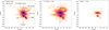 |
Fig. 1 Distribution on the Cartesian X-Z plane of metal-poor ([Fe∕H]<-2 dex, left panel), intermediate metallicity (−2<[Fe∕H]<-1 dex, middle panel), and metal-rich ([Fe/H]>-1 dex, right panel) RRLs. |
2.2 Subset selections
We selected RRLs belonging to the Sgr stream using three different methods, obtaining three distinct subsets:
Ramos et al. (2022) used the Gaia EDR3 catalog (Gaia Collaboration 2021) to identify more than 700 000 candidate members of the Sgr stream based on strict kinematic criteria. We cross-matched our clean sample of RRLs, as defined in Sect. 2.1, with the sample from Ramos et al. (2022) and identified 3865 RRLs in common (Table A.1). In the following discussion, we refer to this sample as RRLS-SGR-R22. Figure B.1 shows the distribution of RRLs in the RRLS-SGR-R22 sample.
-
Vasiliev et al. (2021) developed an N-body model of the disrupting Sgr galaxy within the combined gravitational potential of the MW (with a triaxial halo) and the LMC (with a mass of 1.5 × 10¹¹ M3). This model provides a reasonable fit to many observed properties of the Sgr system. We decided to use it as a reference to select a sample of RRLs with a 5D phase-space distribution as similar as possible to the model’s predictions. To this end, we used the publicly available snapshot of the Vasiliev et al. (2021) model at the present day, which includes 200 000 particles of the simulated Sgr system, providing their Cartesian coordinates, proper motions, distances, and stripping times, defined as the most recent time a particle left a sphere of radius 5 kpc around the Sgr progenitor. We then performed a 5D Cartesian cross-match between the RRLs in our clean sample and the simulated particles using the Cartesian coordinates (X, Y, Z) and proper motions (pmra, pmdec). The tolerance intervals for the cross-match were set as follows: ∆X = 2 kpc, ∆Y = 2 kpc, ∆Z = 2 kpc, ∆pmra = 0.15 mas/yr, and ∆pmdec = 0.15 mas/yr, consistent with the mean errors of 2 kpc for distances, 0.15 mas/yr for pmra, and 0.13 mas/yr for pmdec of the RRLs in the clean sample.
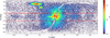
Fig. 2 Density map of the 131 274 RRLs from the clean sample in the Sgr coordinate system (B versus Λ), as defined by Vasiliev et al. (2021). The dashed red lines correspond to B = 20° and B = −20°.
Based on this positional and kinematic match, we assume that the RRLs that have a simulated counterpart likely originated from the Sgr progenitor. We also consider the stripping time of the associated model particle as a reasonable estimate of the stripping time of the matched RRL. This transfer of a label from model particles to real RRLs is not meant to be interpreted on a star-by-star basis. Rather, it is justified in a statistical sense, as particles in the model snapshot that share position and proper motion with the matched RRLs tend to have been stripped around the same epoch. Thus, this approach provides a way to rank different portions of the stream according to the timescale of tidal stripping during the disruption of the Sgr progenitor, similar to the methodology adopted by Limberg et al. (2023), who used the same N -body model as a reference.
This cross-match resulted in a sample of 2377 RRLs, which we refer to as RRLS-SGR-MODEL (Table A.2). Among the RRLs in the RRLS-SGR-MODEL sample, 1926 stars (81%) are also present in the RRLS-SGR-R22 sample, which was selected using completely independent criteria by Ramos et al. (2022). This significant overlap confirms the robustness of our selection procedure, demonstrating that our cross-match with the model data effectively identifies RRLs associated with the Sgr stream. Figure B.2 shows the distributions of RRLs from the RRLS-SGR-MODEL sample alongside the simulated stars from Vasiliev et al. (2021). Compared to the RRLS-SGR-R22 sample, the RRLS-SGR-MODEL sample is more sparsely populated in the region of the leading arm apocenter (Λ ≃ 80°, D ≃ 60 kpc), but it does sample with a handful of RRLs some arms of the stream that are not present in the RRLS-SGR-R22 sample.
-
We performed our own selection of RRLs belonging to the Sgr stream using a slightly modified version of the selection procedure introduced by Ibata et al. (2020), which includes the following steps. From the clean sample of RRLs, we selected stars with distances from the Sun greater than 15 kpc and less than 150 kpc, and with absolute distance errors below 10 kpc. This resulted in a sample of 58 547 stars. As shown in Fig. 2, members of the Sgr stream have Sgr B coordinate within the range [−20°, 20°]. We therefore selected RRLs within this range, yielding a sample of 14 805 stars. We then transformed the Sgr coordinates used in our study, defined in the system introduced by Vasiliev et al. (2021), into the system adopted by Ibata et al. (2020) in the following way:
 (3)
(3)We then applied the equation proposed by Ibata et al. (2020) in the form
 (4)
(4)where we slightly modified the coefficients a3 and a41 resulting in the following values: a1 = 1.1842, a2 = −1.5639 ×π/180, a3 = −0.2, a4 = −2, a5 = −8.0606 × 10⁻⁴, and a6 = 3.2441 × 10⁻⁵. We then selected stars satisfying the criterion |μΛI20 - μΛI20,fit | < 0.6 and obtained a sample of 6738 RRLs. We then selected stars based on μB, adopting the fitted function μBI20,fit (Λ120), which follows the same functional form as μΛI20,fit (ΛI20) in Eq. (4), with the coefficients from Ibata et al. (2020): a1 = −1.2360, a2 = 1.0910 × π/180, a3 = 0.3633, a4 = −1.3412, a5 = 7.3022 × 10⁻³, and a6 = −4.3315 × 10⁻⁵. We retained stars satisfying the criterion |μBI20 - μBI20,fit| < 0.6, resulting in a sample of 5271 RRLs.
The distribution of RRLs selected in this way is shown with red points in Fig. 3, overlaid on the present-day snapshot from the Vasiliev et al. (2021) model (black dots). Panel a shows their distribution in the Cartesian Z versus X plane; panel b presents the distribution of distances versus the Sgr Λ coordinate for the same samples; while panels c and d display the Gaia DR3 proper motions, transformed into Sgr coordinates, μΛ and μB, as functions of Λ. The Sgr coordinates follow the system defined by Vasiliev et al. (2021). Figs. B.1 and B.2, which show the properties of the RRLS-SGR-R22 and RRLS-SGR-MODEL samples, respectively, are arranged in the same way.
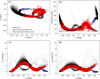
Fig. 3 Distributions of RRLs from the RRLS-SGR-SELECTION sample, obtained through the main selection procedure (red points) and the selection of far-arm stars as described by Eq. (5) (blue points), along with simulated stars from the Vasiliev et al. (2021) model (black dots), shown in the following planes: (a) Cartesian Z versus X, (b) distance versus the Sgr Λ coordinate, (c) proper motion μΛ versus Λ, and (d) proper motion μB versus Λ coordinate. The Sgr coordinates and proper motions are in the system introduced by Vasiliev et al. (2021).
The leading and trailing arms of the Sgr stream are clearly visible in Fig. 3, sampled with more stars and extending to larger distances from the main body along the stream than in the RRLS-SGR-R22 and RRLS-SGR-MODEL samples. However, this approach, as well as the previous ones, is unable to select the RRLs around the apocenter of the trailing arm identified by Sesar et al. (2017a) and noted by Bellazzini et al. (2020) in the region of the globular cluster NGC2419 (see also Belokurov et al. 2014; Davies et al. 2024). In an attempt to include these stars, we applied an additional selection step by choosing, from the clean sample of RRLs, stars with
 (5)
(5)This selection allowed us to identify 25 additional RRLs as candidate members of the Sgr stream (shown with blue points in Fig. 3), located in the lower branch of the bifurcation occurring at the apocenter of the trailing arm, that is, the branch bending back toward the Galactic center. We refer to this sparse sample, which provides insight into the old population in this remote portion of the Sgr stream, as the “far arm.” Together with the 5271 RRLs selected in the previous steps, they form a sample of 5296 RRLs, which we refer to as RRLS-SGR-SELECTION in the following analysis (Table A.3). This selection procedure allowed us to identify 3500 out of 3865 (90%) RRLs from the RRLS-SGR-R22 sample as Sgr stream members, confirming the robustness of our method.
Information on the three datasets selected in steps (1)–(3) is presented in Table 1. Figure 4 shows that the three samples have very similar metallicity distributions and indistinguishable weighted mean metallicity values (see Table 1). The mean metal-licity of RRLs in the Sgr stream, calculated as the mean value of metallicities from the three samples RRLS-SGR-R22, RRLS-SGR-SELECTION, and RRLS-SGR-MODEL used in this study, is [Fe∕H]=−1.62 ± 0.01 dex.
Figure 5 shows the distributions of stars simulated in the Vasiliev et al. (2021) model and RRLs from the RRLS-SGR-MODEL, RRLS-SGR-R22, and RRLS-SGR-SELECTION samples on the μΛ versus Λ plane, color-coded by distances. There is good agreement between the model and all three datasets, confirming that the model successfully reproduces the main features of the Sgr stream as traced by RRLs. While the agreement with the RRLS-SGR-MODEL sample is expected, the consistency with the other two samples provides an independent validation. Additionally, Fig. 5 highlights the different properties and selection effects affecting each of the three samples.
Figure 6 shows the distribution of stars simulated in the Vasiliev et al. (2021) model, along with RRLs from the RRLS-SGR-R22 and RRLS-SGR-SELECTION samples, plotted in the distance versus Λ plane. The squares represent the mean distances as a function of Λ modeled by Hernitschek et al. (2017), based on RRLs from the PS1 survey with distances derived using period-luminosity relations in the visual and near-infrared PS1 bands (Sesar et al. 2017b). The figure demonstrates a good agreement between the distance estimates in this study and the independent results from Hernitschek et al. (2017).
The RRLS-SGR-R22 sample is expected to have a high degree of purity; however, it is limited to −140° ≤ Λ ≤ 150°, and it also lacks stars in the range 5° ≤ Λ ≤ 30° to avoid contamination from stars in the Galactic Disk. Additionally, it does not include RRLs from the far arm of the Sgr stream. The RRLS-SGR-MODEL sample, while less complete and dependent on the Vasiliev et al. (2021) model, provides valuable information on the stripping times of the various portions of the stream. Finally, the RRLS-SGR-SELECTION sample is the most complete, including RRLs in regions much closer to the Galactic disk than RRLS-SGR-R22, and from the far arm, but it also has a higher probability of containing nonmembers of the Sgr stream.
In the following analysis, we primarily present results using RRLS-SGR-SELECTION as the reference sample. However, all results presented in the following sections were, when possible, also cross-checked with the other two samples. Although we do not explicitly report this in each case, the findings were consistently in good agreement. This approach strongly mitigates any potential dependence of the presented results on specific selection criteria or samples.
Subsets of RRLs in the Sgr stream used in this study.
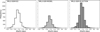 |
Fig. 4 Metallicity distributions of RRLs in the RRLS-SGR-R22, RRLS-SGR-MODEL and RRLS-SGR-SELECTION samples. |
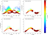 |
Fig. 5 Distributions of stars simulated by the Vasiliev et al. (2021) model and RRLs from the RRLS-SGR-MODEL, RRLS-SGR-R22, and RRLS-SGR-SELECTION samples on the µΛ versus Λ plane, color-coded by distance. The Sgr coordinates and proper motions are given in the system introduced by Vasiliev et al. (2021). |
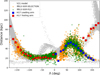 |
Fig. 6 Distributions of stars simulated by the Vasiliev et al. (2021) model (gray points) and RRLs from the RRLS-SGR-R22 (green points) and RRLS-SGR-SELECTION (orange points) samples, in the distance versus Λ plane. Blue and red squares represent the mean distances as a function of Λ in the leading and trailing arms, respectively, as modeled by Hernitschek et al. (2017). The SgrΛ coordinate is given in the system introduced by Vasiliev et al. (2021). |
3 Metallicity of the Sgr stream
3.1 Metallicity gradient in the Sgr stream
In this section, we study the metallicity distribution of RRLs in the Sgr stream. It is important to recall that RRLs do not trace the metallicity gradient of the entire population of the Sgr system, nor of its dominant component, which is likely younger than −810 Gyr and more metal-rich than [Fe/H] - −1.0 dex (de Boer et al. 2015), especially in the main body and in the stream regions closest to it (Bellazzini et al. 2006a; Minelli et al. 2023). On the other hand, since RRLs are mainly old stars (age ≥10 Gyr), and the vast majority of them have [Fe/H] ≤ −1.0 dex, RRLS are useful because they most probably trace the metallicity as it was before the accretion.
The upper panels of Fig. 7 show the distributions of RRLs from the RRLS-SGR-SELECTION sample, color-coded by metallicity. For comparison, the lower panels of Fig. 7 display the distributions of simulated stars from the Vasiliev et al. (2021) model, color-coded by stripping time from the Sgr progenitor. The leading and far arms of the Sgr stream, which, according to the model of Vasiliev et al. (2021), contain stars stripped in earlier epochs, appear visually more metal-poor. This suggests that the metallicity gradient in the Sgr progenitor – with metalrich stars concentrated in the center and metal-poor stars in the halo – was already established at the time of RRLs formation (~10 Gyr ago).
To study the correlation between the epoch at which RRLs were stripped from the Sgr dSph and their metallicities, in Fig. 8, we plot the metallicities of RRLs in the RRLS-SGR-MODEL sample as a function of stripping time, based on the model of Vasiliev et al. (2021). Red squares indicate the median metal-licities in bins containing more than ten RRLs. Only stars with stripping times less than zero, which have already left the sphere with a radius of 5 kpc around the Sgr progenitor (Vasiliev et al. 2021), are shown. We found a weak metallicity gradient of 0.05 ± 0.02 dex/Gyr, determined by performing a linear leastsquares fit to the median metallicity values in bins of stripping time. The fit yields a p-value of 0.026, representing the probability of obtaining the observed gradient under the null hypothesis (i.e., if the true underlying gradient were zero). Since this value is below the conventional 0.05 threshold, we conclude that the metallicity gradient is statistically significant at the 95% confidence level. This result suggests that a metallicity gradient was present in the Sgr progenitor already at very early epochs, with less metal-poor stars concentrated toward the center and more metal-poor stars distributed in the halo.
To analyze the metallicity gradient in the Sgr main body and stream in more detail, we divide the RRLs in the RRLS-SGR-SELECTION sample into four subsets as follows:
Leading arm: 10° ≤ ΛV21 ≤ 180°, 25 ≤ D⊙ ≤ 60 kpc;
Trailing arm: −180° ≤ ΛV21 < −20°, 15 ≤ D⊙ ≤ 75 kpc;
Main body: −20° ≤ ΛV21 < 10°, 20 ≤ D⊙ ≤ 33 kpc;
Far arm: selected as in Eq. (5).
The left panel of Fig. 9 shows the distribution of Sgr substructures in the distance versus Λ plane, while the right panel presents the cumulative distribution functions of RRL metallic-ities for different substructures. Table 2 summarizes the number of RRLs in each substructure along with their mean metallici-ties. These results agree well with the mean metallicities for the main body (−1.60 dex), leading arm (−1.71 dex), and trailing arm (−1.65 dex) reported by Sun et al. (2025), who used photometric metallicities of RRLs derived by Li et al. (2023). Table 3 shows the results of the two-sample Kolmogorov–Smirnov (KS) test comparing the metallicity distributions of RRLs in different substructures. All p-values are significantly below the canonical 0.05 threshold, indicating that the metallicity distributions in different substructures, are statistically different. As evident from Fig. 9 and Table 2, the main body is the most metal-rich substructure of the Sgr stream, followed by the slightly more metal-poor trailing arm, then the leading arm, and finally the far arm, which is significantly more metal-poor. The low metallic-ity of the far arm could potentially be caused by contamination from MW halo RRLs. In the following analysis, we examine and rule out this hypothesis (see the discussion in Sect. 3.4). The discovered trend is in agreement with the findings of Yang et al. (2019), who analyzed the kinematic and chemical properties of ∼3000 Sgr members, including K-giants, M-giants, and blue horizontal branch stars. All three tracers indicate that the trailing arm is, on average, more metal-rich than the leading arm, while the K-giants also show that the far arm is the most metal-poor substructure. Ramos et al. (2022) and Sun et al. (2025) found a similar trend in the metallicity distributions of the main body, leading, and trailing arms, as traced by RRLs.
In Fig. 10, we present the distribution of metallicity as a function of the Sgr Λ coordinate for the trailing and leading arms.
The green and red squares represent the median metallicities of the trailing and leading arms, respectively, calculated for bins containing more than 15 RRLs. We find negligible metallicity gradients of (−0.2 ± 0.3) × 10−3 dex/deg in the trailing arm and of (−1.0 ± 0.5) × 10−3 dex/deg in the leading arm in agreement with previous studies (Ramos et al. 2020; Sun et al. 2025).
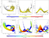 |
Fig. 7 Upper panels: distributions of RRLs from the RRLS-SGR-SELECTION sample in the Cartesian Z versus X plane, the heliocentric distance versus the Sgr Λ coordinate plane, and the proper motion μΛ versus Λ plane, color-coded by metallicity. Lower panels: same distributions but for the sample of simulated stars from Vasiliev et al. (2021), color-coded by time of stripping from the Sgr progenitor. |
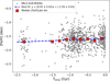 |
Fig. 8 Metallicity as a function of stripping time (Tstrip) for RRLs from the RRLS-SGR-MODEL sample with Tstrip < 0 (gray dots). The red squares indicate median metallicities computed within bins containing more than ten RRLs. The dashed blue line represents the best linear fit to the median metallicity values. |
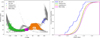 |
Fig. 9 Left panel: distribution of RRLs from different Sgr stream substructures in the distance versus Λ plane. Right panel: cumulative distribution functions of metallicity for RRLs in each substructure. |
Weighted mean metallicity of RRLs in different substructures of the Sgr stream.
Results of the two-sample KS test comparing the metallicity distributions of RRLs in different substructures.
3.2 Bifurcation
Belokurov et al. (2006) discovered two parallel branches in the leading arm of the Sgr stream, commonly referred to as a bifurcation. Later, Koposov et al. (2012) and Navarrete et al. (2017) identified a similar bifurcation, comprising faint and bright branches, in the trailing arm. It has also been reported that the faint branch is slightly more metal-poor than the bright branch (Koposov et al. 2012; Ramos et al. 2022), with the bright branch being the more populated one (branch A, in the nomenclature of Belokurov et al. 2006) and the faint branch the sparser one, running in parallel at higher declination (branch B, in the same nomenclature of Belokurov et al. 2006).
Several models have been proposed to explain this feature, but its origin remains a subject of debate, as none appears fully satisfactory when compared to observations. Fellhauer et al. (2006) suggested that the bifurcation results from precession induced on the Sgr progenitor by the asphericity of the MW halo. Peñarrubia et al. (2010) proposed that a rotating, disk-like Sgr progenitor could have produced the bifurcation. Other hypotheses include intrinsic anisotropy within the Sgr progenitor (Law & Majewski 2010), or the presence of a secondary, independent satellite accreted along with the Sgr galaxy (Law & Majewski 2010; Koposov et al. 2012; Davies et al. 2024). Ramos et al. (2022), using the model of Vasiliev et al. (2021) as a reference for interpretation, conclude that the two branches are primarily populated by stars stripped during different perigalactic passages of the Sgr progenitor: the faint, more metal-poor branch during the antepenultimate passage, and the bright branch during the penultimate passage (see also Koposov et al. 2012). An unspecified perturbation is invoked to eject the stars into slightly different orbits during the two passages, thereby producing the observed sky misalignment of the branches.
Ramos et al. (2022) showed that the two parallel branches of the stream can also be traced with RRLs, although they appear much less evident, likely due to the relative sparsity of RRLs compared to other stellar tracers in the stream (see their Fig. B.3). Given their relatively low numbers and the narrow range of ages and metallicities they sample, RRLs may not be the most suitable tracers for investigating differences between the branches. However, since all the RRLs in the RRLS-SGR-R22 sample have been assigned probabilities of belonging to either the faint (ProbFaint) or the bright branch (ProbBright) by Ramos et al. (2022), it may still be useful to compare the metallicities of RRLs in the two branches.
For our analysis, we applied selection criteria consistent with those adopted in Sect. 3.1 to identify the faint and bright branches of the leading and trailing arms:
Faint leading branch: 10° ≤ ΛV21 ≤ 180°, ProbFaint >0.2, ProbFaint > ProbBright;
Bright leading branch: 10° ≤ ΛV21 ≤ ProbBright > 0.2, ProbFaint < ProbBright;
Faint trailing branch: −180° ≤ ΛV21 < ProbFaint > 0.2, ProbFaint > ProbBright;
Bright trailing branch: −180° ≤ ΛV21 < ProbBright > 0.2, ProbFaint < ProbBright;
Table 4 presents the number of RRLs in each of these subsets along with their mean metallicity, while Fig. 11 shows the metal-licity distributions. The faint branch of the leading arm is only 0.01 dex more metal-poor than the bright branch, whereas the faint branch of the trailing arm is 0.01 dex more metal-rich than the bright branch. The metallicity distributions are statistically indistinguishable, according to a KS test. This result is consistent with the findings of Ramos et al. (2020).
Differences in metallicity along the stream are usually interpreted as the result of stars being stripped at different times, each sampling distinct layers of the Sgr progenitor’s age and metallicity gradient. In this context, it is worth noting that the difference in stripping times proposed to explain the bifurcation (Ramos et al. 2022) leads to only a negligible difference in the RRL metallicity distributions between the two branches, to be compared with the statistically significant differences detected between the trailing, leading and far arms discussed in Sect. 3.1. However, this does not seem to shed any light in the problem of the physical origin of the bifurcation.
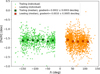 |
Fig. 10 Distribution of metallicity as a function of the Sgr Λ coordinate for RRLs in the trailing (green points) and leading (orange points) arms. Dark green and red squares represent median metallicities computed in bins containing more than 15 RRLs for the trailing and leading arms, respectively. |
Weighted mean metallicity of RRLs in the faint and bright branches of the Sgr stream.
3.3 Main body
In Sect. 3.1, we identified 2445 RRLs from the RRLS-SGR-SELECTION sample as belonging to the main body of the Sgr stream. For each RRL in this sample, we calculated the radial distance from the center of the Sgr core using the Euclidean distance between the Galactocentric Cartesian coordinates of the Sgr center ({17.9, 2.6, –6.6}, Vasiliev et al. 2021) and the coordinates of the star, as derived in Sect. 2.1. Figure 12 illustrates the metallicity of RRLs in the main body as a function of radius. The dashed blue line represents the weighted mean metallicity of RRLs in the main body, [Fe/H] = −1.58 ± 0.31 dex. The magenta squares indicate the median metallicities calculated for each bin containing more than ten RRLs. We find a metallicity gradient of −0.008 ± 0.005 dex/kpc, with more metal-rich RRLs located closer to the center of the Sgr progenitor. However, this gradient is not statistically significant ( p-value = 0.198), indicating that the observed trend is consistent with no real correlation between metallicity and radial distance.
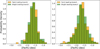 |
Fig. 11 Metallicity distributions of RRLs in the faint (orange) and bright (green) branches of the trailing (left panel) and leading arms (right panel) of the Sgr stream. |
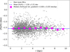 |
Fig. 12 Metallicity distribution as a function of radial distance from the center of the Sgr core for RRLs in the RRLS-SGR-SELECTION sample belonging to the main body. The blue line represents the weighted mean metallicity of RRLs in the main body, while the magenta squares indicate the median metallicities calculated for each bin containing more than ten RRLs. |
3.4 Far arm
We analyzed 25 RRLs belonging to the far arm of the Sgr stream, selected as described in Eq. (5). The weighted mean metallicity of RRLs in the far arm is [Fe/H] = −1.98 ± 0.37 dex, which is approximately 0.3 dex lower than the mean metallicity of the RRLs in the leading arm. This makes the far arm the most metalpoor structure of the Sgr stream. This finding aligns with the expectation that more metal-poor RRLs were originally located in the outskirts of the Sgr progenitor and, hence, were stripped during the earlier stages of Sgr accretion.
Figure 13 presents the histogram (green bins) of the metal-licity distribution of RRLs in the far arm. Two distinct peaks are visible, approximately at [Fe/H] = −2.4 dex and [Fe/H] = −1.7 dex. This bimodal distribution could be due either to contamination from RRLs in the MW field or to the possibility that RRLs in the far arm were stripped from the Sgr progenitor at different epochs during the accretion process. We compare this distribution with the metallicity distribution of RRLs in the MW halo located at distances corresponding to those of the Sgr far arm RRLs (61–84 kpc). We excluded from this sample RRLs located in the Sgr far arm and within 10° of the LMC and SMC centers, resulting in a sample of 1118 RRLs. Their weighted mean metallicity is [Fe/H] = −1.83 ± 0.33 dex. The metallic-ity distribution of this halo sample is shown with orange bins in Fig. 13. Although one of the peaks in the far arm distribution is close to the peak of the halo sample, the two distributions appear visually distinct. A two-sample KS test between the MW halo stars and the metal-rich ([Fe/H] > –2 dex) subset of the Sgr far arm yields a p-value of 0.067, indicating that the two samples could be drawn from the same distribution. In contrast, the KS test between the halo stars and the metal-poor ([Fe/H] < –2 dex) subset of the Sgr far arm returns a p-value of 10−7, confirming that these two datasets are statistically different. However, the current sample size of far arm RRLs is too small to draw firm conclusions about the origin of its bimodal metallicity distribution.
 |
Fig. 13 Metallicity distributions of RRLs in the far arm of the Sgr stream (green bins) and in the MW halo at distances between 61 and 84 kpc (orange bins). The dashed dark orange line indicates the weighted mean metallicity of the MW halo sample. |
4 Conclusions
In this study, we analyzed the Sgr stream as traced by RRLs from the Gaia DR3 catalog (Clementini et al. 2023). Photometric metallicities for these RRLs were computed by Muraveva et al. (2025), and accurate distances were determined using the reddening-free PWZ relation from Garofalo et al. (2022). The new metallicity and distance estimates enable a more precise characterization of the Sgr stream’s structure and metallicity gradient.
We find a good agreement between the distances and kinematic distribution of the RRLs in our sample and those of the stars simulated in the Vasiliev et al. (2021) model, which accounts for the gravitational potential of the MW and the LMC. Using the simulated stars from the Vasiliev et al. (2021) model, we were able to calculate the metallicity gradient as a function of the time of stripping of the stars from the Sgr progenitor. We find a mild but statistically significant metallicity gradient of 0.05 ± 0.02 dex/Gyr, with more metal-poor stars being stripped at earlier epochs. This result confirms the existence of a metallicity gradient in the Sgr progenitor at the epoch of formation of RRLs, with metal-rich stars concentrated toward the center and metalpoor stars distributed in the outer regions of the Sgr progenitor.
We find that the main body is the most metal-rich substructure of the Sgr stream ([Fe/H] = −1.58 ± 0.31 dex), followed by the slightly more metal-poor trailing arm ([Fe/H] = −1.64 ± 0.28 dex), then the leading arm ([Fe/H] = −1.69 ± 0.31 dex), and finally the far arm ([Fe/H] = −1.98 ± 0.37 dex), which is the most metal-poor substructure of the Sgr stream. Although the mean metallicities of RRLs in different substructures are formally consistent within the uncertainties, a two-sample KS test indicates that the metallicity distributions are statistically different, suggesting the presence of an underlying metallicity gradient among the substructures. We also find almost negligible metallicity gradients as a function of Λ, with values of (−0.2 ± 0.3) × 10−3 dex/deg in the trailing arm and (−1.0 ± 0.5) × 10−3 dex/deg in the leading arm. These results are in agreement with previous studies (Ramos et al. 2020; Sun et al. 2025). We analyzed the bifurcation in the trailing and leading arms (Belokurov et al. 2006; Koposov et al. 2012). We find that the difference in mean metallicities between the faint and bright branches is approximately 0.01 dex, which is not statistically significant. We conclude that the metallicity difference between the faint and bright branches of the Sgr stream is not confirmed based on the RRLs in our sample. This result is consistent with the findings of Ramos et al. (2020).
To the best of our knowledge, in this study we analyzed for the first time the metallicity gradient as a function of radial distance in the Sgr main body as traced by RRLs. We find a weak metallicity gradient of −0.008 ± 0.005 dex/kpc, with more metalrich RRLs located closer to the center of the Sgr progenitor. However, the observed gradient is not statistically significant, indicating that the true gradient may be consistent with zero. We also analyzed 25 RRLs in the far arm of the Sgr stream and found a bimodal distribution in metallicity, with peaks at [Fe/H]=−2.4 dex and [Fe/H]=−1.7 dex. This bimodal distribution could be due to contamination of the far arm sample by MW RRLs. Alternatively, the bimodality might reflect different epochs of stripping of RRLs from the Sgr progenitor in the far arm. However, our sample of RRLs in the far arm is not large enough to draw robust conclusions about the origin of this two-peaked metallicity distribution.
The Sgr stream is one of the most significant contributors to the MW’s stellar halo. The mean metallicity of RRLs in the Sgr stream, calculated as the mean value of metallicities from the three samples used in this study, is [Fe/H]=−1.62 ± 0.01 dex. This value is in good agreement but slightly more metal-poor than the median metallicity of the MW halo RRLs, [Fe/H]=−1.55 ± 0.01 dex (Crestani et al. 2021). At the same time, the Sgr stream’s RRLs are less metal-poor than those in some ultra-faint streams, such as the Orphan stream, which has a mean metallicity of [Fe/H]=−1.80 ± 0.06 dex (Prudil et al. 2021). This reflects Sgr’s higher progenitor mass (4.3 × 10⁷ Mθ, Pace 2024) and higher overall metallicity (see the discussion on the mass–metallicity relation of galaxies as traced with RRLs in Bellazzini et al. 2025). A more extensive study of the structure and metallicity gradient of the Sgr stream, as traced with RRLs, will be made possible with the arrival of Gaia Data Release 4, currently foreseen for the second half of 2026.
Acknowledgements
Acknowledgements. We sincerely thank the anonymous referee for their thoughtful and constructive comments, which helped improve the clarity and quality of this manuscript. Support to this study has been provided by INAF MiniGrant (PI: Tatiana Muraveva), by the Agenzia Spaziale Italiana (ASI) through contract ASI 2018-24-HH.0 and its Addendum 2018-24-HH.1-2022, and by Premiale 2015, MIning The Cosmos – Big Data and Innovative Italian Technology for Frontiers Astrophysics and Cosmology (MITiC; P.I.B.Garilli). MB acknowledge the support to this study by the PRIN INAF Mini Grant 2023 (Ob.Fu. 1.05.23.04.02 – CUP C33C23000960005) CHAM – Chemo-dynamics of the Accreted Halo of the Milky Way (P.I.: M. Bellazzini). MB acknowledges the financial support by the project LEGO – Reconstructing the building blocks of the Galaxy by chemical tagging (P.I.: A. Mucciarelli), granted by the Italian MUR through contract PRIN 2022LLP8TK_001. This work uses data from the European Space Agency mission Gaia (https://www. cosmos.esa.int/gaia), processed by the Gaia Data Processing and Analysis Consortium (DPAC; https://www.cosmos.esa.int/web/gaia/dpac/consortium). Funding for the DPAC has been provided by national institutions, in particular the institutions participating in the Gaia Multilateral Agreement.
Data availability
Full Tables A.1–A.3 are available at the CDS via https://cdsarc.cds.unistra.fr/viz-bin/cat/J/A+A/701/A228
Appendix A Datasets
Parameters of the 3865 RRLs in the RRLS-SGR-R22 sample (extract).
Parameters of the 2377 RRLs in the RRLS-SGR-MODEL sample (extract).
Parameters of the 5296 RRLs in the RRLS-SGR-SELECTION sample (extract).
Appendix B Plots
In this section we present the distributions of RRLs from the RRLS-SGR-R22 (Fig. B.1) and RRLS-SGR-MODEL (Fig. B.2) samples, overlaid on the present-day snapshot from the Vasiliev et al. (2021) model. Panel (a) shows the distributions in the Cartesian Z versus X plane; panel (b) presents the distribution of distances versus the Sgr Λ coordinate for the same samples; while panels (c) and (d) display the Gaia DR3 proper motions, transformed into Sgr coordinates, μΛ and μB, as functions of Λ.
 |
Fig. B.1 Distributions of RRLs from the RRLS-SGR-R22 sample (green points) and simulated stars from the Vasiliev et al. (2021) model (black dots) shown in the following planes: (a) Cartesian Z versus X, (b) distance versus the Sgr Λ coordinate, (c) proper motion in the Sgr system µΛ versus Λ, and (d) µB versus Λ coordinate. The Sgr coordinates and proper motions are in the system introduced by Vasiliev et al. (2021). |
 |
Fig. B.2 Distributions of RRLs from the RRLS-SGR-MODEL sample (orange points) and simulated stars from the Vasiliev et al. (2021) model (black dots) shown in the following planes: (a) Cartesian Z versus X, (b) distance versus the Sgr Λ coordinate, (c) proper motion in the Sgr system µΛ versus Λ, and (d) µB versus Λ coordinate. The Sgr coordinates and proper motions are in the system introduced by Vasiliev et al. (2021). |
References
- Antoja, T., Ramos, P., Mateu, C., et al. 2020, A&A, 635, L3 [NASA ADS] [CrossRef] [EDP Sciences] [Google Scholar]
- Bayer, M., Starkenburg, E., Thomas, G. F., et al. 2025, A&A, 701, A117 [NASA ADS] [CrossRef] [EDP Sciences] [Google Scholar]
- Bellazzini, M., Correnti, M., Ferraro, F. R., Monaco, L., & Montegriffo, P. 2006a, A&A, 446, L1 [NASA ADS] [CrossRef] [EDP Sciences] [Google Scholar]
- Bellazzini, M., Newberg, H. J., Correnti, M., Ferraro, F. R., & Monaco, L. 2006b, A&A, 457, L21 [NASA ADS] [CrossRef] [EDP Sciences] [Google Scholar]
- Bellazzini, M., Ibata, R., Malhan, K., et al. 2020, A&A, 636, A107 [NASA ADS] [CrossRef] [EDP Sciences] [Google Scholar]
- Bellazzini, M., Muraveva, T., & Garofalo, A. 2025, A&A, 698, L10 [NASA ADS] [CrossRef] [EDP Sciences] [Google Scholar]
- Belokurov, V., Zucker, D. B., Evans, N. W., et al. 2006, ApJ, 642, L137 [Google Scholar]
- Belokurov, V., Koposov, S. E., Evans, N. W., et al. 2014, MNRAS, 437, 116 [NASA ADS] [CrossRef] [Google Scholar]
- Bobrick, A., Iorio, G., Belokurov, V., et al. 2024, MNRAS, 527, 12196 [Google Scholar]
- Bono, G., Caputo, F., Castellani, V., et al. 2003, MNRAS, 344, 1097 [Google Scholar]
- Carretta, E., Bragaglia, A., Gratton, R., D’Orazi, V., & Lucatello, S. 2009, A&A, 508, 695 [NASA ADS] [CrossRef] [EDP Sciences] [Google Scholar]
- Catelan, M. 2004, in IAU Colloq. 193: Variable Stars in the Local Group, eds. D. W. Kurtz, & K. R. Pollard, Astronomical Society of the Pacific Conference Series, 310, 113 [Google Scholar]
- Chou, M.-Y., Majewski, S. R., Cunha, K., et al. 2007, ApJ, 670, 346 [NASA ADS] [CrossRef] [Google Scholar]
- Clementini, G., Gratton, R., Bragaglia, A., et al. 2003, AJ, 125, 1309 [CrossRef] [Google Scholar]
- Clementini, G., Ripepi, V., Molinaro, R., et al. 2019, A&A, 622, A60 [NASA ADS] [CrossRef] [EDP Sciences] [Google Scholar]
- Clementini, G., Ripepi, V., Garofalo, A., et al. 2023, A&A, 674, A18 [NASA ADS] [CrossRef] [EDP Sciences] [Google Scholar]
- Crestani, J., Fabrizio, M., Braga, V. F., et al. 2021, ApJ, 908, 20 [Google Scholar]
- Cui, X.-Q., Zhao, Y.-H., Chu, Y.-Q., et al. 2012, Res. Astron. Astrophys., 12, 1197 [Google Scholar]
- Davies, E. Y., Belokurov, V., Monty, S., & Evans, N. W. 2024, MNRAS, 529, L73 [Google Scholar]
- de Boer, T. J. L., Belokurov, V., Beers, T. C., & Lee, Y. S. 2014, MNRAS, 443, 658 [NASA ADS] [CrossRef] [Google Scholar]
- de Boer, T. J. L., Belokurov, V., & Koposov, S. 2015, MNRAS, 451, 3489 [Google Scholar]
- Dierickx, M. I. P., & Loeb, A. 2017, ApJ, 836, 92 [NASA ADS] [CrossRef] [Google Scholar]
- Fardal, M. A., van der Marel, R. P., Law, D. R., et al. 2019, MNRAS, 483, 4724 [NASA ADS] [CrossRef] [Google Scholar]
- Fellhauer, M., Belokurov, V., Evans, N. W., et al. 2006, ApJ, 651, 167 [NASA ADS] [CrossRef] [Google Scholar]
- Gaia Collaboration (Brown, A. G. A., et al.) 2018, A&A, 616, A1 [NASA ADS] [CrossRef] [EDP Sciences] [Google Scholar]
- Gaia Collaboration (Brown, A. G. A., et al.) 2021, A&A, 649, A1 [NASA ADS] [CrossRef] [EDP Sciences] [Google Scholar]
- Gaia Collaboration (Vallenari, A., et al.) 2023, A&A, 674, A1 [NASA ADS] [CrossRef] [EDP Sciences] [Google Scholar]
- Garofalo, A., Delgado, H. E., Sarro, L. M., et al. 2022, MNRAS, 513, 788 [NASA ADS] [CrossRef] [Google Scholar]
- Gibbons, S. L. J., Belokurov, V., & Evans, N. W. 2017, MNRAS, 464, 794 [NASA ADS] [CrossRef] [Google Scholar]
- GRAVITY Collaboration (Abuter, R., et al.) 2018, A&A, 615, L15 [NASA ADS] [CrossRef] [EDP Sciences] [Google Scholar]
- Hayes, C. R., Majewski, S. R., Hasselquist, S., et al. 2020, ApJ, 889, 63 [Google Scholar]
- Helmi, A., & White, S. D. M. 2001, MNRAS, 323, 529 [NASA ADS] [CrossRef] [Google Scholar]
- Hernitschek, N., Sesar, B., Rix, H.-W., et al. 2017, ApJ, 850, 96 [NASA ADS] [CrossRef] [Google Scholar]
- Ibata, R. A., & Lewis, G. F. 1998, ApJ, 500, 575 [Google Scholar]
- Ibata, R. A., Gilmore, G., & Irwin, M. J. 1994, Nature, 370, 194 [Google Scholar]
- Ibata, R., Bellazzini, M., Thomas, G., et al. 2020, ApJ, 891, L19 [NASA ADS] [CrossRef] [Google Scholar]
- Jurcsik, J., & Kovacs, G. 1996, A&A, 312, 111 [Google Scholar]
- Kaiser, N., Burgett, W., Chambers, K., et al. 2010, SPIE Conf. Ser., 7733, 77330E [Google Scholar]
- Koposov, S. E., Belokurov, V., Evans, N. W., et al. 2012, ApJ, 750, 80 [NASA ADS] [CrossRef] [Google Scholar]
- Law, D. R., & Majewski, S. R. 2010, ApJ, 714, 229 [Google Scholar]
- Li, X.-Y., Huang, Y., Liu, G.-C., Beers, T. C., & Zhang, H.-W. 2023, ApJ, 944, 88 [NASA ADS] [CrossRef] [Google Scholar]
- Limberg, G., Queiroz, A. B. A., Perottoni, H. D., et al. 2023, ApJ, 946, 66 [NASA ADS] [CrossRef] [Google Scholar]
- Liu, G. C., Huang, Y., Zhang, H. W., et al. 2020, ApJS, 247, 68 [NASA ADS] [CrossRef] [Google Scholar]
- Longmore, A. J., Fernley, J. A., & Jameson, R. F. 1986, MNRAS, 220, 279 [NASA ADS] [Google Scholar]
- Madore, B. F., Hoffman, D., Freedman, W. L., et al. 2013, ApJ, 776, 135 [Google Scholar]
- Majewski, S. R., Skrutskie, M. F., Weinberg, M. D., & Ostheimer, J. C. 2003, ApJ, 599, 1082 [NASA ADS] [CrossRef] [Google Scholar]
- Martínez-Delgado, D., Aparicio, A., Gómez-Flechoso, M. Á., & Carrera, R. 2001, ApJ, 549, L199 [CrossRef] [Google Scholar]
- Martínez-Delgado, D., Gómez-Flechoso, M. Á., Aparicio, A., & Carrera, R. 2004, ApJ, 601, 242 [CrossRef] [Google Scholar]
- Minelli, A., Bellazzini, M., Mucciarelli, A., et al. 2023, A&A, 669, A54 [NASA ADS] [CrossRef] [EDP Sciences] [Google Scholar]
- Monaco, L., Bellazzini, M., Bonifacio, P., et al. 2007, A&A, 464, 201 [NASA ADS] [CrossRef] [EDP Sciences] [Google Scholar]
- Morgan, S. M., Wahl, J. N., & Wieckhorst, R. M. 2007, MNRAS, 374, 1421 [NASA ADS] [CrossRef] [Google Scholar]
- Mullen, J. P., Marengo, M., Martínez-Vázquez, C. E., et al. 2021, ApJ, 912, 144 [NASA ADS] [CrossRef] [Google Scholar]
- Muraveva, T., Palmer, M., Clementini, G., et al. 2015, ApJ, 807, 127 [Google Scholar]
- Muraveva, T., Delgado, H. E., Clementini, G., Sarro, L. M., & Garofalo, A. 2018, MNRAS, 481, 1195 [Google Scholar]
- Muraveva, T., Giannetti, A., Clementini, G., Garofalo, A., & Monti, L. 2025, MNRAS, 536, 2749 [Google Scholar]
- Navarrete, C., Belokurov, V., Koposov, S. E., et al. 2017, MNRAS, 467, 1329 [NASA ADS] [Google Scholar]
- Neeley, J. R., Marengo, M., Bono, G., et al. 2017, ApJ, 841, 84 [Google Scholar]
- Neeley, J. R., Marengo, M., Freedman, W. L., et al. 2019, MNRAS, 490, 4254 [Google Scholar]
- Nemec, J. M., Cohen, J. G., Ripepi, V., et al. 2013, ApJ, 773, 181 [CrossRef] [Google Scholar]
- Oria, P.-A., Ibata, R., Ramos, P., Famaey, B., & Errani, R. 2022, ApJ, 932, L14 [NASA ADS] [CrossRef] [Google Scholar]
- Pace, A. B. 2024, arXiv e-prints [arXiv:2411.07424] [Google Scholar]
- Peñarrubia, J., Belokurov, V., Evans, N. W., et al. 2010, MNRAS, 408, L26 [NASA ADS] [Google Scholar]
- Price-Whelan, A. M. 2017, J. Open Source Softw., 2 [Google Scholar]
- Prudil, Z., Hanke, M., Lemasle, B., et al. 2021, A&A, 648, A78 [NASA ADS] [CrossRef] [EDP Sciences] [Google Scholar]
- Prudil, Z., Kunder, A., Dékány, I., & Koch-Hansen, A. J. 2024, A&A, 684, A176 [NASA ADS] [CrossRef] [EDP Sciences] [Google Scholar]
- Ramos, P., Mateu, C., Antoja, T., et al. 2020, A&A, 638, A104 [EDP Sciences] [Google Scholar]
- Ramos, P., Antoja, T., Yuan, Z., et al. 2022, A&A, 666, A64 [NASA ADS] [CrossRef] [EDP Sciences] [Google Scholar]
- Rimoldini, L., Holl, B., Audard, M., et al. 2019, A&A, 625, A97 [NASA ADS] [CrossRef] [EDP Sciences] [Google Scholar]
- Ripepi, V., Molinaro, R., Musella, I., et al. 2019, A&A, 625, A14 [NASA ADS] [CrossRef] [EDP Sciences] [Google Scholar]
- Sarbadhicary, S. K., Heiger, M., Badenes, C., et al. 2021, ApJ, 912, 140 [Google Scholar]
- Sesar, B., Hernitschek, N., Dierickx, M. I. P., Fardal, M. A., & Rix, H.-W. 2017a, ApJ, 844, L4 [Google Scholar]
- Sesar, B., Hernitschek, N., Mitrovic´, S., et al. 2017b, AJ, 153, 204 [NASA ADS] [CrossRef] [Google Scholar]
- Sollima, A., Cacciari, C., Arkharov, A. A. H., et al. 2008, MNRAS, 384, 1583 [Google Scholar]
- Soszyn´ski, I., Udalski, A., Szyman´ski, M. K., et al. 2014, Acta Astron., 64, 177 [Google Scholar]
- Soszyn´ski, I., Udalski, A., Wrona, M., et al. 2019, Acta Astron., 69, 321 [NASA ADS] [Google Scholar]
- Sun, S., Wang, F., Zhang, H., et al. 2025, ApJ, 979, 213 [Google Scholar]
- Thomas, G. F., Famaey, B., Ibata, R., Lüghausen, F., & Kroupa, P. 2017, A&A, 603, A65 [NASA ADS] [CrossRef] [EDP Sciences] [Google Scholar]
- Vasiliev, E., Belokurov, V., & Erkal, D. 2021, MNRAS, 501, 2279 [NASA ADS] [CrossRef] [Google Scholar]
- Vera-Ciro, C., & Helmi, A. 2013, ApJ, 773, L4 [Google Scholar]
- Wang, F., Zhang, H. W., Xue, X. X., et al. 2022, MNRAS, 513, 1958 [NASA ADS] [CrossRef] [Google Scholar]
- Yang, C., Xue, X.-X., Li, J., et al. 2019, ApJ, 886, 154 [NASA ADS] [CrossRef] [Google Scholar]
- Yanny, B., Rockosi, C., Newberg, H. J., et al. 2009, AJ, 137, 4377 [Google Scholar]
- York, D. G., Adelman, J., Anderson, Jr., J. E., et al. 2000, AJ, 120, 1579 [NASA ADS] [CrossRef] [Google Scholar]
- Zinn, R., & West, M. J. 1984, ApJS, 55, 45 [Google Scholar]
This modification of the Ibata et al. (2020) selection criteria was made to adjust the fit to the distribution of the Sgr stream as traced by the Gaia DR3 data, since the original formula by Ibata et al. (2020) was based on the Gaia DR2 data.
All Tables
Results of the two-sample KS test comparing the metallicity distributions of RRLs in different substructures.
Weighted mean metallicity of RRLs in the faint and bright branches of the Sgr stream.
All Figures
|
Fig. 1 Distribution on the Cartesian X-Z plane of metal-poor ([Fe∕H]<-2 dex, left panel), intermediate metallicity (−2<[Fe∕H]<-1 dex, middle panel), and metal-rich ([Fe/H]>-1 dex, right panel) RRLs. |
| In the text | |
|
Fig. 2 Density map of the 131 274 RRLs from the clean sample in the Sgr coordinate system (B versus Λ), as defined by Vasiliev et al. (2021). The dashed red lines correspond to B = 20° and B = −20°. |
| In the text | |
|
Fig. 3 Distributions of RRLs from the RRLS-SGR-SELECTION sample, obtained through the main selection procedure (red points) and the selection of far-arm stars as described by Eq. (5) (blue points), along with simulated stars from the Vasiliev et al. (2021) model (black dots), shown in the following planes: (a) Cartesian Z versus X, (b) distance versus the Sgr Λ coordinate, (c) proper motion μΛ versus Λ, and (d) proper motion μB versus Λ coordinate. The Sgr coordinates and proper motions are in the system introduced by Vasiliev et al. (2021). |
| In the text | |
|
Fig. 4 Metallicity distributions of RRLs in the RRLS-SGR-R22, RRLS-SGR-MODEL and RRLS-SGR-SELECTION samples. |
| In the text | |
|
Fig. 5 Distributions of stars simulated by the Vasiliev et al. (2021) model and RRLs from the RRLS-SGR-MODEL, RRLS-SGR-R22, and RRLS-SGR-SELECTION samples on the µΛ versus Λ plane, color-coded by distance. The Sgr coordinates and proper motions are given in the system introduced by Vasiliev et al. (2021). |
| In the text | |
|
Fig. 6 Distributions of stars simulated by the Vasiliev et al. (2021) model (gray points) and RRLs from the RRLS-SGR-R22 (green points) and RRLS-SGR-SELECTION (orange points) samples, in the distance versus Λ plane. Blue and red squares represent the mean distances as a function of Λ in the leading and trailing arms, respectively, as modeled by Hernitschek et al. (2017). The SgrΛ coordinate is given in the system introduced by Vasiliev et al. (2021). |
| In the text | |
|
Fig. 7 Upper panels: distributions of RRLs from the RRLS-SGR-SELECTION sample in the Cartesian Z versus X plane, the heliocentric distance versus the Sgr Λ coordinate plane, and the proper motion μΛ versus Λ plane, color-coded by metallicity. Lower panels: same distributions but for the sample of simulated stars from Vasiliev et al. (2021), color-coded by time of stripping from the Sgr progenitor. |
| In the text | |
|
Fig. 8 Metallicity as a function of stripping time (Tstrip) for RRLs from the RRLS-SGR-MODEL sample with Tstrip < 0 (gray dots). The red squares indicate median metallicities computed within bins containing more than ten RRLs. The dashed blue line represents the best linear fit to the median metallicity values. |
| In the text | |
|
Fig. 9 Left panel: distribution of RRLs from different Sgr stream substructures in the distance versus Λ plane. Right panel: cumulative distribution functions of metallicity for RRLs in each substructure. |
| In the text | |
|
Fig. 10 Distribution of metallicity as a function of the Sgr Λ coordinate for RRLs in the trailing (green points) and leading (orange points) arms. Dark green and red squares represent median metallicities computed in bins containing more than 15 RRLs for the trailing and leading arms, respectively. |
| In the text | |
|
Fig. 11 Metallicity distributions of RRLs in the faint (orange) and bright (green) branches of the trailing (left panel) and leading arms (right panel) of the Sgr stream. |
| In the text | |
|
Fig. 12 Metallicity distribution as a function of radial distance from the center of the Sgr core for RRLs in the RRLS-SGR-SELECTION sample belonging to the main body. The blue line represents the weighted mean metallicity of RRLs in the main body, while the magenta squares indicate the median metallicities calculated for each bin containing more than ten RRLs. |
| In the text | |
|
Fig. 13 Metallicity distributions of RRLs in the far arm of the Sgr stream (green bins) and in the MW halo at distances between 61 and 84 kpc (orange bins). The dashed dark orange line indicates the weighted mean metallicity of the MW halo sample. |
| In the text | |
|
Fig. B.1 Distributions of RRLs from the RRLS-SGR-R22 sample (green points) and simulated stars from the Vasiliev et al. (2021) model (black dots) shown in the following planes: (a) Cartesian Z versus X, (b) distance versus the Sgr Λ coordinate, (c) proper motion in the Sgr system µΛ versus Λ, and (d) µB versus Λ coordinate. The Sgr coordinates and proper motions are in the system introduced by Vasiliev et al. (2021). |
| In the text | |
|
Fig. B.2 Distributions of RRLs from the RRLS-SGR-MODEL sample (orange points) and simulated stars from the Vasiliev et al. (2021) model (black dots) shown in the following planes: (a) Cartesian Z versus X, (b) distance versus the Sgr Λ coordinate, (c) proper motion in the Sgr system µΛ versus Λ, and (d) µB versus Λ coordinate. The Sgr coordinates and proper motions are in the system introduced by Vasiliev et al. (2021). |
| In the text | |
Current usage metrics show cumulative count of Article Views (full-text article views including HTML views, PDF and ePub downloads, according to the available data) and Abstracts Views on Vision4Press platform.
Data correspond to usage on the plateform after 2015. The current usage metrics is available 48-96 hours after online publication and is updated daily on week days.
Initial download of the metrics may take a while.