| Issue |
A&A
Volume 701, September 2025
|
|
|---|---|---|
| Article Number | A165 | |
| Number of page(s) | 20 | |
| Section | Interstellar and circumstellar matter | |
| DOI | https://doi.org/10.1051/0004-6361/202555688 | |
| Published online | 12 September 2025 | |
ANTIHEROES-PRODIGE: Quantifying the connection from the envelope to the disk with the IRAM 30 m telescope and NOEMA
I. Infalling streamers in L1448N
1
Max-Planck-Institut für Astronomie, Königstuhl 17, 69117 Heidelberg, Germany
2
Max-Planck-Institut für extraterrestrische Physik, Giessenbach-strasse 1, 85748 Garching, Germany
3
Department of Physics and Astronomy, University of Rochester, Rochester, NY, 14627, USA
4
European Southern Observatory, Karl-Schwarzschild-Strasse 2 85748 Garching bei München, München, Germany
5
Taiwan Astronomical Research Alliance (TARA), Taiwan
6
Institute of Astronomy and Astrophysics, Academia Sinica, No. 1, Sec. 4, Roosevelt Road, Taipei 10617, Taiwan
7
Institut de Radioastronomie Millimétrique (IRAM), 300 rue de la Piscine, 38406, Saint-Martin d’Hères, France
8
Joint ALMA Observatory, Alonso de Córdova 3107, Vitacura, Santiago, Chile
9
National Radio Astronomy Observatory, 520 Edgemont Road, Charlottesville, VA 22903, USA
10
SKA Observatory, Jodrell Bank, Lower Withington, Macclesfield SK11 9FT, UK
11
Laboratoire d’astrophysique de Bordeaux, Univ. Bordeaux, CNRS, B18N, allée Geoffroy Saint-Hilaire, 33615 Pessac, France
12
Centro de Astrobiología (CAB), CSIC-INTA, Ctra. de Torrejón a Ajalvir, km 4, 28850 Torrejón de Ardoz, Spain
13
IPAG, Université Grenoble Alpes, CNRS, 38000 Grenoble, France
14
Zentrum für Astronomie der Universität Heidelberg, Institut für Theoretische Astrophysik, Albert-Ueberle-Str. 2, 69120 Heidelberg, Germany
15
Observatorio Astronómico Nacional (IGN), Alfonso XII 3, 28014 Madrid, Spain
16
Space Research Institute, Austrian Academy of Sciences, Schmiedl-str. 6, 8042 Graz, Austria
★ Corresponding author: This email address is being protected from spambots. You need JavaScript enabled to view it.
Received:
27
May
2025
Accepted:
22
July
2025
Abstract
Context. Star formation is a hierarchical process that ranges from molecular clouds to individual protostars. In particular, it remains to be understood how infalling asymmetric structures (streamers) that deliver new material to protostellar systems are connected to the surrounding envelope.
Aims. We investigated the connection between the cloud material at scales of 10 000–300 au toward L1448N in the Perseus starforming region, which hosts three young Class 0/I protostellar systems (IRS3A, IRS3B, and IRS3C).
Methods. Sensitive molecular line observations taken with the Institut de Radioastronomie Millimetrique (IRAM) 30 m telescope and the Northern Extended Millimeter Array (NOEMA) at 1.4 mm were used to study the kinematic properties in the region that is traced by the molecular lines (C18O, SO, DCN, and SO2). The temperature in the region was estimated using transitions of c-C3H2.
Results. Several infalling streamers are associated with the protostellar systems. Some of them are traced by C18O and DCN, and one of them is bright in SO and SO2. The kinematic properties of the former streamers are consistent with the velocities observed at large envelope scales of 10 000 au, while the kinematics of the latter case are different. The masses and infall rates of the streamers are 0.01 M⊙ and 0.01-0.1 M⊙ and 10-6 M⊙ yr-1 and 5-18 × 10-6 M⊙ yr-1 for IRS3A and IRS3C. The envelope mass in the L1448N region is ≈16 M⊙, and the mass of a single streamer is thus lower than the envelope mass (<1%). Compared to the estimated mass of the protostellar systems, however, a single streamer could deliver up to 1 and 8-17% of mass toward IRS3A (M* ≈ 1.2 M⊙) and IRS3C (M* ≈ 1 M⊙), respectively.
Conclusions. The rotational signatures of structures in L1448N are all connected, from the large-scale envelope and infalling streamers to the rotation of all three disks. Two of the three Class 0/I protostellar systems are still fed by this surrounding material, which can be associated with the remnant envelope. We also found a streamer that is bright in SO and SO2 toward IRS3C. This might be connected to a nearby sulfur reservoir. Further studies are required to study the diverse chemical compositions and the origin of the streamers.
Key words: astrochemistry / line: profiles / stars: formation
© The Authors 2025
 Open Access article, published by EDP Sciences, under the terms of the Creative Commons Attribution License (https://creativecommons.org/licenses/by/4.0), which permits unrestricted use, distribution, and reproduction in any medium, provided the original work is properly cited.
This article is published in open access under the Subscribe to Open model.
Open Access funding provided by Max Planck Society.
1 Introduction
It is essential to investigate the earliest and most deeply embedded stages of star formation to understand (proto)stellar evolution, the properties of surrounding protoplanetary disks, and the formation of embedded planets. A protostellar system in the Class 0/I stage during low-mass star formation is still surrounded by a large mass reservoir that allows further mass growth (Evans et al. 2009; Dunham et al. 2014). Understanding how the envelope material feeds protostellar systems requires multiscale observations on scales from the large envelope to the small disk (Pineda et al. 2023).
A spherically symmetric collapse of an isolated core was first considered in early theoretical models of the formation of a solartype star (e.g., Larson 1969; Penston 1969; Shu 1977). Sensitive observations with a high spatial resolution from the infrared to radio wavelengths over the past decades have revealed that star formation is a complex process in which the environment and asymmetries have to be taken into account, such as filamentary structures in molecular clouds (André et al. 2014; Hacar et al. 2023), multiplicity (Offner et al. 2023), protoplanetary disks (Miotello et al. 2023), chemical diversity (Ceccarelli et al. 2023), and streamers (Pineda et al. 2020). We use the definition that a streamer is an asymmetric structure with kinematically confirmed infall motions. More recent models and simulations that for example include turbulence and magnetic fields also show asymmetries at all scales relevant for star formation (e.g., Walch et al. 2009; Offner et al. 2010; Ballesteros-Paredes et al. 2015; Seifried et al. 2015; Chira et al. 2018; Kuffmeier et al. 2019; Kuznetsova et al. 2022; Kuffmeier 2024).
Asymmetric infalling streamers have been identified in interferometric data in various molecular lines, such as HC3N (Pineda et al. 2020; Valdivia-Mena et al. 2024), CO (Ginski et al. 2021), 13CO (Gupta et al. 2024), C18O (Yen et al. 2014; Flores et al. 2023; Kido et al. 2023; Mercimek et al. 2023; Cacciapuoti et al. 2024; Kido et al. 2025), HCO+ (Yen et al. 2019; Garufi et al. 2022), C2H (Tanious et al. 2024), H2CO (Valdivia-Mena et al. 2022; Podio et al. 2024), and CH3 CN (Fernández-López et al. 2023), and deuterated species such as DCN (Hsieh et al. 2023; Gieser et al. 2024, Cortes et al. subm.). The origin and effects of these infalling structures, including mass infall rates and potential shocks at the landing sites in the disk, have yet to be thoroughly investigated. Most importantly, the connection between streamers and the surrounding envelope material remains unclear because the investigation is challenged by the limited field of view (FOV) and the insufficient line sensitivity of current interferometers.
Recently, a double infalling streamer structure, referred to as the bridge, has been found toward the protostar IRS3A, which is located in L1448N (Gieser et al. 2024). The L1448N starforming complex is located in the Perseus molecular cloud at a distance of 288 ± 6 ± 13 pc (with statistical and systemic uncertainties, respectively, Zucker et al. 2018). This region contains three Class 0/I protostellar systems (IRS3A, IRS3B, and IRS3C) that host a single, triple, and binary system, respectively (Tobin et al. 2018). While IRS3B and IRS3C are Class 0 systems, it is unclear whether IRS3A is in the Class 0 or I stage (e.g., Ciardi et al. 2003). In the following, we therefore refer to all systems as Class 0/I. Continuum observations with a high angular resolution with the Atacama Large Millimeter/submillimeter Array (ALMA) have revealed a ring and spiral-arm structures in the disks of IRS3A and IRS3B, respectively, while the two protostars in the IRS3C binary system each have a compact disk (Tobin et al. 2016; Reynolds et al. 2021, 2024). An overview of the dust continuum distribution of L1448N is presented in Fig. 1. It also includes the orientation of the outflows in the systems (Lee et al. 2016; Reynolds et al. 2021; Gieser et al. 2024; Dunham et al. 2024). The outflow in the IRS3B multiple system can be associated with the protostar IRS3B-C (Reynolds et al. 2021), while currently available data for IRS3C prevent us from distinguishing which protostar in the binary drives the outflow (Tobin et al. 2018).
The three Class 0/I systems of L1448N are target regions of the survey called PROtostars & DIsks: Global Evolution (PRODIGE). This large program with the Northern Extended Millimeter Array (NOEMA) is part of the Max-Planck IRAM Observatory program (MIOP). The NOEMA continuum and molecular line observations at 1.4 mm probe spatial scales down to 300 au at the distance of the Perseus molecular cloud (1″ angular resolution) and trace the environment of the protostel-lar systems. PRODIGE observations of DCN (3 - 2) revealed an extended gas bridge that surrounds systems IRS3A and IRS3B. The bridge is infalling onto IRS3A (Gieser et al. 2024). The gas bridge was even larger in other molecular line tracers such as C18O (2 - 1) and H2CO (30,3 - 20,2). The spatial filtering in the NOEMA observations due to missing short-baseline data prevented us from studying the connection of the gas bridge to the environment and from estimating masses and infall rates of the streamers, however.
To complement the NOEMA data of PRODIGE, we are carrying out the IRAM 30 m telescope large program called “quantifying the connection from the envelope to the disk with MIOP-PRODIGE” (ANTIHEROES). The sensitive single-dish maps allow us to study the large-scale properties of the molecular gas that surrounds the protostellar systems from a few 10 000–3600 au (12″). The combination of the interferometric and single-dish observations allow us to recover the flux on all scales, and thus, we are able to reliably estimate molecular column densities and kinematic properties to 300 au scales for the entire PRODIGE sample.
In this work, we analyze the connection of infalling streamers to the larger-scale material from 36 000 (120″) to 300 au (1″) scales based on a combination of IRAM 30 m telescope and NOEMA molecular line observations to demonstrate the potential of the combined data. The paper is organized as follows: Section 2 contains a description of the PRODIGE and ANTIHEROES data reduction, and the combination of both datasets. The analysis of the molecular line data is presented in Sect. 3, and our results are further discussed in Sect. 4. Our conclusions are summarized in Sect. 5.
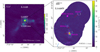 |
Fig. 1 Continuum images toward L1448N. The left panel shows large-scale 1.1 mm continuum emission of L1448 (Enoch et al. 2006). The beam size is shown in the bottom left corner. The map size of the IRAM 30 m observations is highlighted by the dashed gray rectangle. The right panel shows the NOEMA 1.4 mm continuum of L1448N with contour levels at 5, 25, 60, 120, 200 times σcont with σcont = 0.78 mJy beam-1. The triangles and white labels mark the positions of individual protostars (Tobin et al. 2016), and the pink cross marks the recently detected source IRS3-ALMA (Looney et al. 2025). The bipolar outflow directions launched by the three protostellar systems are marked by red and blue arrows, including the blueshifted outflow lobe that is launched by L1448-mm toward the southeast. The synthesized beam of the NOEMA continuum data is shown in the bottom left corner. The scale bars in the two panels are shown in the top left corner. |
2 Observations
In this section, we explain the data reduction of the NOEMA and IRAM 30 m datasets and the merging of the data. The molecular line properties (quantum numbers, rest-frequency ν, upper energy level Eu/kB, and Einstein A-coefficient Aul) of all transitions we analyzed, and the angular resolution and noise properties of the observations, are summarized in Table A.1.
2.1 NOEMA continuum and molecular line data
The PRODIGE project (program id: L19MB, PIs: P. Caselli and Th. Henning) covers L1448N with NOEMA in the 1.4 mm band. Three individual pointings toward the protostellar systems IRS3A, IRS3B, and IRS3C were obtained from December 2019 to October 2022 in the C- and D-array configurations. The projected baselines range from 15.9 up to 402 m. The frequency coverage of the wideband data is 214.7-222.8 GHz in the lower sideband (LSB) and 230.2-238.3 GHz in the upper sideband (USB) at a channel width of 2 MHz (≈2.7 km s-1 at 1.4 mm). A total of 39 high spectral resolution units with smaller bandwidths (narrowband data) were placed within the LSB and USB frequency ranges with a channel width of 62.5 kHz (≈0.09 km s-1 at 1.4 mm). A summary of all molecular transitions covered by the narrowband data that we analyzed is presented in Table A.1.
A detailed description of the NOEMA data-calibration procedure using CLIC1, including phase self-calibration using MAPPING, of the IRS3A and IRS3B PRODIGE data is presented in Sect. 2.1 in Gieser et al. (2024). For the purpose of this work, we applied the same method to the additional IRS3C pointing. The three NOEMA pointings overlap sufficiently within their primary beam for us to combine all pointings into a mosaic (as described in Sect. 2.2 in Gieser et al. 2024).
Using MAPPING, we imaged the continuum and SO2 NOEMA data with robust weighting (robust parameter of one) and natural weighting, respectively, and cleaned them with the Hogbom algorithm (Högbom 1974) because the emission is compact (Figs. 1 and 2). Because SO2 is not detected in the IRAM 30 m data (Fig. 2), we only used the NOEMA data for this molecular transition, as only noise would be added in the data merging. For all other transitions we analyzed (Table A.1), extended emission is detected in the IRAM 30 m data. It is therefore crucial for these transitions to merge the two datasets to recover missing flux from the spatial filtering. The remaining molecular line data were first merged with the IRAM 30 m data, imaged with natural weighting, and then cleaned with the SDI algorithm (Steer et al. 1984), which takes the extended emission into account (as described further in Sect. 2.3). We applied primary beam correction with a primary beam size of ≈22" at 1.4 mm to all data. To increase the signal-to-noise ratio (S/N) of the spectral line data, we rebinned the narrowband data to a common channel width of 0.1 km s-1.
The continuum mosaic data were cleaned down to three times the theoretical noise with a support mask around the emission of the three protostellar systems. The synthesized beam (θmaj × θmin) of the continuum data is 0.″91 × 0.″73 with a position angle (PA) of 18°. The continuum noise level, σcont, is 0.78 mJy beam-1 as estimated from an emission-free area. The SO2 NOEMA data were cleaned down to the theoretical noise and no support mask. The imaging and cleaning of the remaining molecular line data that were first merged with the IRAM 30 m data is further presented in Sect. 2.3.
2.2 Line data from the IRAM 30 m telescope
To avoid missing extended line emission that may be resolved out by the interferometer, we combined the NOEMA data with complementary zero-spacing spectral line observations from the IRAM 30 m telescope using the Eight MIxer Receiver (EMIR), which covers the same frequency range as the NOEMA data (program code 096-23, PI: C. Gieser). These observations of L1448N are the pilot project for the ongoing ANTIHEROES large program (program code 162-24, PI: C. Gieser), which includes the remaining protostellar systems of the entire PRODIGE sample. The fast Fourier transform spectrometer (FTS) backend provides a channel width of 50 kHz (~0.07kms-1).
The IRAM 30 m observations of L1448N were carried out in the on-the-fly (OTF) mode in February and April 2024. The central position of the map is αJ2000 = 3h25m36s and δJ2000 = 30°45′30″. The OTF maps have a size of 120″ × 120″, and the region was observed in zigzag scanning mode (scanning speed 5″ s-1) in right ascension and declination. The reference offset position (αJ2000 = 3h26m40s and δJ2000 = 30°50′0″) was selected based on the nondetection of 13CO emission in the COordinated Molecular Probe Line Extinction Thermal Emission (COMPLETE) survey data (Ridge et al. 2006). Pointing and focus settings were checked and corrected every ≈1 and ≈2h, respectively, on nearby and bright sources.
The single-dish data were reduced with the CLASS package. In individual spectra, baseline subtraction was carried out by fitting a first-order polynomial around the emission lines. The data were converted from antenna temperature ( ) into main-beam temperature (TMB) using
  with a forward efficiency Feff = 0.94 and a main-beam efficiency Beff = 0.632. The single-dish spectral line data were also rebinned to 0.1 km s-1 to match the spectral grid of the NOEMA data. Standalone IRAM 30 m data cubes were created using xy_map with a pixel scale of 3″. The half-power beam width (HPBW) is ≈12″ at 1.4 mm, which corresponds to 3600 au at the distance of L1448N.
2.3 Data merging of the line data
We merged the interferometric and single-dish spectral line data using the uv_short task in MAPPING. The merged line data were imaged with natural weighting and cleaned without a support mask down to the theoretical noise using the SDI algorithm. As a second threshold, we set a maximum number of 5000 clean components per channel to avoid overcleaning channels with very extended emission. The pixel scale was set to 0.15″, and the angular resolution was ≈1″ (300 au at the distance of L1448N).
The channel width δv, beam size, and noise level of the IRAM 30 m (θ, σline,30m) and merged or NOEMA (θmaj × θmin (PA), σline) spectral line data are summarized for all transitions in Table A.1. The line sensitivity was ≈100 mK and ≈0.4 K for the IRAM 30 m and merged data, respectively. This dataset provides sensitive molecular line observations from scales of 36 000 au (120″) to 300 au (1″), which is crucial for understanding the origin of molecular gas, such as streamers, that feeds the protostellar systems. The importance of merging the IRAM 30 m data with the NOEMA observations is further evaluated in Appendix B, where we compare the spatial distribution and individual spectra of DCN (3 - 2) and C18O (2 - 1). The comparison shows that more than 90% is filtered out in the PRODIGE C18O (2 - 1) NOEMA data compared to the merged ANTIHEROES-PRODIGE data. Most transitions (CO, C18O, SO, DCN, and c-C3HC2) we studied show extended emission. It is therefore crucial to include short-spacing data to properly analyze the kinematic properties and measure reliable fluxes.
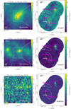 |
Fig. 2 Line-integrated intensity map of C18O (2 - 1), SO (65 - 54), and SO2 (42,2 - 31,3) of the IRAM 30 m data (left) and merged or NOEMA data (right). The line-integrated intensity is shown in color in all panels. The contours and arrows are the same as in Fig. 1. The synthesized beam of the line and continuum data is shown in the bottom left and right corners, respectively. The scale bars are shown in the top left corner in all panels. In the right panels, distinct structures (bridge and stick) seen in molecular emission are indicated by dashed ellipses. |
3 Results
We present our analysis of the standalone single-dish data, and the combined NOEMA + IRAM 30 m molecular line data. In Sect. 3.1 we separate the complex line profiles of C18O and SO2 in order to extract infalling streamers and connect their kinematic properties to the larger-scale environment. In Sect. 3.2 we use c-C3H2 to estimate the temperature in the L1448N region. In Sect. 3.3 we infer the source velocity and central mass of the IRS3C system. A streamline model is applied in Sect. 3.4 to the C18O and SO2 streamers found toward IRS3C. The mass and infall rates of the C18O and SO2 streamers of IRS3C and DCN streamers of IRS3A (Gieser et al. 2024) are inferred in Sect. 3.5.
3.1 Kinematic properties of the molecular gas
3.1.1 Spatial morphology of C18O
The line-integrated (v=1-11 km s-1) intensity maps of the C18O (2 - 1) transition of the IRAM 30 m and merged data are presented in Fig. 2. In the IRAM 30 m map, C18O is brightest toward the locations of the three protostellar systems with a NW-SE elongation. In the merged data, this elongated feature shows even more substructure. The bridge structure discovered previously in the PRODIGE data in which IRS3A and IRS3B are embedded is clearly detected (Gieser et al. 2024).
North of IRS3A there is an elongated feature that we refer to as the stick in the following. This structure is nearby the IRS3-ALMA source that was recently detected in millimeter continuum by Looney et al. (2025). Although these authors argued that this source is most likely a background galaxy, the stick structure might be associated with the source given the spatial vicinity. IRS3-ALMA might therefore also be a very faint and young protostar or a prestellar core associated with L1448N. It is beyond the scope of this work to further investigate the nature of IRS3-ALMA.
Elongated structures surround the IRS3C system. The feature connecting IRS3A/B to IRS3C was previously reported by Volgenau et al. (2006) in C18O (1 - 0) emission (their Fig. 1). Based on the orientation along the outflow direction of IRS3C, the morphology indicates that C18O traces the remnant envelope that is carved out by the outflow.
3.1.2 Spatial morphology and channel maps of SO and SO2
The line-integrated (v = 2-6 km s-1) intensity maps of the SO (65 - 54) and SO2 (42,2 - 31,3) transitions of the IRAM 30 m and merged and NOEMA data, respectively, are presented in Fig. 2. In the single-dish data, SO2 is not detected, while the large-scale distribution of SO peaks toward IRS3C, but also east and west of the L1448N region, where no known protostars are located. In the NOEMA data, however, SO2 is bright toward IRS3C, with a bright arc toward the south of the protostellar system. This elongated arc structure is also detected in bright SO emission.
The channel maps from 2.4 to 5.5 km s-1 toward IRS3C for the SO (65 - 54) and SO2 (42,2 - 31,3) transitions are presented in Fig. 3. For comparison, the red- and blueshifted morphology of the outflow is highlighted using CO (2 - 1) merged data of ANTIHEROES-PRODIGE (Table A.1). There is compact SO and SO2 emission at high velocities toward the IRS3C proto-stellar system that rotates southwest (blueshifted) to northeast (redshifted), which is consistent with high angular resolution C18O data that trace the circumbinary material (Tobin et al. 2018). The redshifted side is strongly blended by extended emission, however: In both tracers, a blob from 3.6 km s-1 to 4.6 km s-1 lies north of the IRS3C continuum and the elongated arc structure toward the southwest (marked in the 4.2 km s-1 channel in Fig. 3). In the SO channel map, extended SO emission also lies close to the region, with velocities between 4.3 and 4.8 km s-1. The emission of the SO blob disappears at 4.7 and 4.8 km s-1, which might be due to absorption against the extended component because it is still detected in the SO2 channel maps. At higher velocities, the blob again becomes bright. The extended emission of SO is known to be abundant in the core envelope because it was also detected in starless and prestel-lar cores (Swade 1989; Spezzano et al. 2017; Vastel et al. 2018; Harju et al. 2020; Lattanzi et al. 2020; Rodríguez-Baras et al. 2021). Although SO is brighter and morphologically more complex, we performed the following kinematic analysis on SO2 because it lacks additional extended emission.
3.1.3 Gaussian decomposition and clustering
In the following, we analyze the kinematic properties of the molecular gas, which has a complex spatial morphology (Fig. 2) in C18O and in sulfur-bearing species (SO and SO2). We study the nature of asymmetric infalling streamers and the connection to the surrounding envelope material in more detail. The dynamics of the infalling gas bridge toward IRS3A have been analyzed in detail using DCN (3 - 2) emission by Gieser et al. (2024) (see also Fig. B.2). While the previous NOEMA-only data could not be used to analyze brighter and more extended molecular emission, such as C18O, the complementary ANTIHEROES data allow us a detailed kinematic analysis over a large area. We applied the same method as presented in Gieser et al. (2024) to the C18O (2 - 1) single-dish and merged data, and the SO2 (42,2 - 31,3) NOEMA data to infer the large-scale kinematic properties of the L1448N envelope and the smaller-scale properties toward IRS3C.
To obtain the kinematic properties, we fit up to three Gaussian velocity components with the pyspeckit package (Ginsburg et al. 2022) to each position in which the peak S/N in that spectrum was higher than 5. For further details of the method, we refer to Gieser et al. (2024), and a summary is presented in Appendix C.
Following the method by Gieser et al. (2024), we used the tool called density-based spatial clustering of applications with noise (DBSCAN) of the Python package scikit-learn (Pedregosa et al. 2011) to extract individual cluster from the dataset of the extracted velocity components. The input was the position (x,y) and peak velocity 3 of all velocity components after quality assessment (Appendix C). We note that the line width and amplitude were not used as an input, but were used to confirm that the clustering results provided reliable results not only in the velocity, but also in line width and amplitude maps. The main clusters relevant for this work are presented in Fig. 4, and the remaining clusters as well as data points discarded by DBSCAN are shown in Fig. C.2.
On large scales such as traced by the IRAM 30 m data, C18O has a velocity gradient from east (redshifted, C18O (IRAM 30 m) cluster 1) to west (blueshifted, C18O (IRAM 30 m) cluster 2), indicating rotation of the large-scale envelope material (left panel in Fig. 4). The protostellar systems are oriented along the rotation axis of this large-scale motion, that is, they are located at the change in the velocities from red- to blueshifted. This large-scale motion is consistent with the rotation of the disks (Tobin et al. 2018; Reynolds et al. 2021). The infalling DCN bridge also shows the same velocity pattern, with the northern redshifted streamer in the east and the southern blueshifted streamer in the west (Gieser et al. 2024). The agreement with the large-scale C18O velocity map thus implies that the infalling material from the gas bridge originates from the large-scale environment. We further discuss this result in Sect. 4.2. Toward the protostellar systems, the line width also increases, with ∆v up to 1.5 km s-1, while in the surrounding environment ∆v <0.5km s-1. An increase like this in the line width along the streamer toward the protostellar system is found toward other streamers such as IRS3A (Gieser et al. 2024) and Per-emb-50 (Valdivia-Mena et al. 2022).
The large-scale envelope rotation is also seen in the higher angular resolution C18O dataset (C18O (merged) cluster 1). The redshifted side of the infalling bridge toward IRS3A can also be extracted in the merged C18O dataset (C18O (merged) cluster 6). We note that due to the large number of data points and the complex line profiles close to the infalling bridge, it is not possible to extract the blue side of the IRS3A bridge in C18O, even though it is evident in the integrated intensity map (Fig. 2). In addition to the rotation of the envelope, an extended emission feature surrounds IRS3C (C18O (merged) cluster 5), where velocities become more blueshifted as the system is approached from the south. The DCN bridge around IRS3A showed a very similar behavior, that is, the velocities become more red- and blueshifted closer to the protostar. This is evidence for infall motions.
The NOEMA SO2 clustering results extract the arc structure toward IRS3C (SO2 (NOEMA) cluster 1) where the emission becomes more redshifted as the system is approached. In higher-resolution ALMA data, Artur de la Villarmois et al. (2023) detected this extended arc in SO and SO2 emission (with transitions at higher upper energy levels of 48-95 K). This suggests that along the arc itself, the gas is denser and/or hotter than in the rest of the gas. The C18O and SO2 asymmetric structures (C18O (merged) cluster 5 and SO2 (NOEMA) cluster 1) we extracted from this clustering method and their infall motions onto IRS3C are further characterized in Sect. 3.4.
 |
Fig. 3 Channel maps of SO 65 - 54 (top, merged data) and SO2 42,2 - 31,3 (bottom, NOEMA-only data) toward L1448 IRS3C. The green color map shows the line intensity with the velocity of the channel in km s-1 labeled in the bottom right. The black contours are the same as in Fig. 1. The dashed red and solid blue contours indicate the CO (2 - 1) integrated intensity of the red- and blueshifted outflow launched by IRS3C. The integration ranges are 5.9-27 km s-1 and 2-3.4 km s-1 (narrow range to avoid foreground contamination) with contour levels at 0.1, 0.3, 0.5, and 0.7 and 0.5, 0.7, and 0.9 times the peak-integrated intensity, respectively. In the top left panel, the black scale bar in the top right corner indicates a spatial scale of 1 000 au. The synthesized beam of the line and continuum data are shown in the bottom left and right corners, respectively. In each panel, the scale is set from a minimum brightness temperature of -0.3 K to a maximum of 7 K. The IRS3C source velocity is 3.8 km -1 (Sect. 3.3). |
 |
Fig. 4 Main clusters extracted with DBSCAN. The velocity, peak intensity, and line width are shown in color in the top, central, and bottom panels, respectively. The contours and arrows are the NOEMA 1.4 mm continuum with the same levels as in Fig. 1. In cluster 1 of each analyzed dataset, the synthesized beam of the line and continuum data is shown in the bottom left and right corner, respectively, and scale bars are shown in the top left corner. The remaining clusters are shown in Fig. C.2. |
3.2 Temperature distribution in L1448N derived from c-C3H2
While hot corino sources in the PRODIGE sample show a plethora of emission lines by complex organic molecules (Hsieh et al. 2024; Busch et al. 2025), the PRODIGE spectral setup typically only covers one transition of smaller molecules. One of the exceptions is c-C3H2, for which three transitions are detected in the PRODIGE+30m data in the L1448N region (Table A.1). The velocity-integrated intensity maps (integrated between 3 and 7km s-1) of the IRAM 30 m and merged data are presented in Fig. D.1.
The emission of the three c-C3 H2 transitions (Fig. D.1) is spatially extended in the 30 m data, where it embeds the three protostellar systems, similar to the distribution of C18O. In the high-resolution NOEMA+30m data, the gas bridge, the stick, and the elongated envelope surrounding IRS3C are traced. The extended emission of c-C3H2 suggests that L1448N is a source of warm carbon-chain chemistry (WCCC; even though c-C3H2 is the cyclic isomer), as suggested previously by Sakai et al. (2009). The authors found a high abundance (>10-9) of C4H derived from single-dish observations and proposed that L1448N is a candidate WCCC source.
The underlying excitation conditions, such as rotation temperature and column density, can be inferred by fitting the radiative transfer equation of the rotational transitions. We used the eXtended CASA Line Analysis Software Suite (XCLASS, Möller et al. 2017, version 1.4.3) to fit the observed IRAM 30 m and merged the spectral line data of c-C3 H2. We applied the same method to the two datasets as explained in detail in Appendix D. Although the spectral line profiles of c-C3H2 show multiple components in some locations (e.g., close to the protostars; Fig. C.1), we chose to fit the observed line profiles with only one velocity component in order to obtain the average excitation conditions in the region. The resulting best-fit parameter maps (Trot, N, ∆v, v) of c-C3H2 are presented in Fig. 5.
The mean excitation temperature in the region is 10 and 14 K in the 30 m and merged data, respectively, indicating that the molecular gas is still cold in the L1448N region over a large area. The merged data shows areas with enhanced temperatures, however, for example, toward the IRS3B disk with temperatures higher than 30 K. The triple system that is embedded in the disk efficiently heats the surrounding gas. The northern envelope material of IRS3C has higher temperatures as well (25 K), which is gas that is heated along the cavity walls of the outflow.
The mean column density in the two datasets is similar, at ≈2×1013 cm-2, but the merged data spatially resolve regions with a higher column density toward the protostellar systems and the surrounding envelope material. Notably, the stick is located very close to IRS3-ALMA (a projected distance of ≈1″, which corresponds to ≈300 au) and also shows higher temperatures and column densities in the merged data. Although we modeled only one c-C3H2 emission component, the line width and velocity maps are similar to those extracted from the more sophisticated kinematic analysis of C18O in Sect. 3.1. Thus, C18O and c-C3H2 trace the same molecular gas components (a spectrum comparing the line profile of molecular analyzed in this work toward all three protostellar systems is shown in Fig. C.1). In Sect. 3.5 we use the temperature determined by the XCLASS fitting of c-C3H2 in order to estimate the mass of infalling streamers and the L1448N envelope.
3.3 Systemic velocity and mass of IRS3C
In order to test whether the structures detected toward IRS3C in C18 O and SO2 (Fig. 4) are due to gravitational infall using streamline models (Pineda et al. 2020, Sect. 3.4), the precise source velocity and the central mass of IRS3C have first to be determined. We estimated the source velocity using DCN (3 - 2) emission following the approach by Gieser et al. (2024). DCN is only weakly detected toward the continuum peak position of IRS3C (Fig. 6), but the spectral line profile is not as complex as other species, such as C18O and SO2 (Fig. C.1). We fit two Gaussian velocity components to the DCN (3 - 2) spectral profile and assigned the brighter component to the IRS3C source velocity, at vLSR = 3.81 ± 0.05 km s-1 ■ Despite its low S/N, the second component was included in the fit to avoid biasing the fitted velocity of the brighter component. The peak of the brighter component coincides with the peak emission of other molecular transitions (Fig. C.1) and therefore is a good estimate of the IRS3C source velocity.
The central mass can be estimated from fitting the position velocity (PV) diagram of molecular lines that trace the disk rotation. The C18O (2 - 1) transition was used for IRS3A (Gieser et al. 2024), but the emission around the IRS3C system is too complex and receives a significant distribution from the surrounding envelope material (Fig. 2). We used the SO2 (42,2 - 31,3) transition to estimate the central mass, but because it is faint, we were not able to fit the PV data (Fig. 7). A match by eye of the observations can still provide an estimate of the mass (see also, e.g., Reynolds et al. 2021; Valdivia-Mena et al. 2022). Given the low S/N of the SO2 PV diagram, more sophisticated PV diagram modeling including rotation and infall is needed, but this is beyond the scope of this work. When we extracted the PV diagram using the pvextractor package (Ginsburg et al. 2015), the blueshifted SO2 velocities appeared to be roughly compatible with an inclination-corrected mass of ≈1 M⊙ (Fig. 7). The position angle and inclination of the disk were taken from Reynolds et al. (2024). For comparison, we also show Keplerian models for the inclination-corrected masses of 0.5 M⊙ and 2 M⊙.
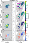 |
Fig. 5 Parameter maps of c-C3 H2 (rotation temperature, column density, FWHM line width, and peak velocity) of the IRAM 30 m (left) and merged (right) data. The contours and arrows are the same as in Fig. 1. The beams of the line and continuum data are shown in the bottom left and right corners, respectively. The scale bars are indicated in the top left corner. |
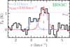 |
Fig. 6 Spectrum of DCN (3 - 2) extracted from the IRS3C continuum peak position The observed spectrum is shown in black, and a two-Gaussian velocity componen fi s hown in bue and red. The dashed purple line marks the 3σline level. The source velocity estimated from the red componen is indicated by the vertical dashed line. |
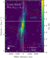 |
Fig. 7 Position velocity diagram of SO2 (42,2 - 31,3) extracted along the disk orientation of IRS3C. The black contours show the 4, 8, and 16σline levels. The red line shows the profile for a Keplerian disk of 1 M⊙ inclined by 50°, and for comparison, the dotted cyan and green lines show profiles for 0.5 M⊙ and 2 M⊙, respectively. A spectral and spatial resolution element (0.1 km s-1 ×283 au) is indicated in the bottom left corner. |
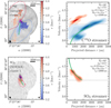 |
Fig. 8 Streamline models toward IRS3C. In the left panels, the line-integrated intensity and the velocities of the structure are shown in gray and color, respectively. The trajectory of the best-match streamline model is shown in green. The contours are the NOEMA 1.4 mm continuum with the same levels as in Fig. 1. The beam of the line and continuum data are shown in the bottom left and right corners, respectively. A scale bar is shown in the top right corner. In the right panels, we indicate the velocity distribution extracted from the areas by dotted ellipses (left) in red or blue, and the best-match streamline model is shown in green. The source velocity of IRS3C (3.8 km s-1) is indicated by the horizontal dashed line. |
3.4 Streamline model
We combined the observed velocity profiles of the C18O and SO2 asymmetric structures (C18O (merged) cluster 5 and SO2 (NOEMA) cluster 1) in Fig. 4) that showed signs of infall motions toward IRS3C, and the determined source velocity and central mass (Sect. 3.3). We tested with this whether the velocities were consistent with gravitational infall toward IRS3C using a streamline model. The analytical solutions (Mendoza et al. 2009) and the applications to infalling streamers are described in detail in Pineda et al. (2020) and are implemented in the Python package velocity_tools3. In short, the streamline model follows the trajectory of a particle in the rotating envelope and is infalling toward the central gravitational sink, that is, the protostellar system.
We ran a grid of models in which we varied the radial separation r0, initial position (θ0, φ0), radial velocity v0 = v(r0), and angular velocity (Ω0) of the particle. We set the rotation of the system to the observed rotation of the circumbinary envelope (Tobin et al. 2018). We note that the angular resolution is not sufficient to spatially resolve the disks of each binary, and we therefore treated the system as one. This also implies that we were unable to determine whether the streamers feed only one of the protostars in the binary or both.
The observed velocity profiles as a function of projected distance from the protostar are shown in the right panel in Fig. 8. The velocities on the blue side of the C18O structure and the SO2 structure become more blue- and redshifted, respectively, as the protostars are approached. For the redshifted side of the C18O structure, however, the velocity becomes more redshifted with distance from the protostar, which is opposite to what is expected from an infalling structure. Because only the line-of-sight velocity component can be observed, however, it might still be infalling. Figure 8 shows the best-match trajectory projected along the plane of the sky on the left and the observed and streamline velocity profile for the C18O and SO2 streamers on the right.
For the blue C18O and SO2 infalling structures, the trajectory and velocity profile in the streamline model match very well. For C18O, no cluster matches the SO2 streamer velocity profile. This might be due to the high spectral complexity of C18O line profiles toward the protostellar systems (Fig. C.1). IRS3C is the first example that shows asymmetric infall from the remnant envelope (C18O) with an additional streamer (bright in SO and SO2) that cannot be directly connected to the envelope material.
Source and streamer properties.
3.5 Streamer mass and infall rates
As reported by Gieser et al. (2024), both the red and blue side of the DCN bridge showed infall motions toward IRS3A. Because no short-spacing data were available at the time, no mass infall rates were determined. A comparison of the NOEMA-only and merged DCN data is presented in Appendix B. The DCN bridge surrounding IRS3A is not affected by spatial filtering, and we therefore use the kinematic results by Gieser et al. (2024) below to estimate the mass and infall rates of the streamers toward IRS3A. For IRS3C, we estimate the mass and infall rates of the C18O and SO2 streamers found in this work (Fig. 8).
Molecular column density (N) maps of the C18O and DCN streamers in IRS3C and IRS3A, respectively, were calculated using an optically thin approximation (Eq. (80) in Mangum & Shirley 2015) within the Python package molecular_columns4. For the excitation temperature, we used Trot from the c-C3H2 map, assuming T — 10 K in all pixels without an available c-C3H2 temperature estimate. The integrated intensity was calculated using the Gaussian-fit results (intensity and line width) of the corresponding cluster. The abundance ratio X of C18O/H2 and DCN/H2 were assumed to be 1.8 × 10⁻⁷ (Frerking et al. 1982; Wilson & Rood 1994) and 2.4 × 10⁻¹⁰ (Hsieh et al. 2023), respectively. To compare the streamer masses with the total envelope mass traced by the IRAM 30 m C18O data, we applied the same method as for the column density calculation using the C18O-integrated intensity map (Fig. 2) and the temperature from the c-C3H2 single-dish map assuming T — 10 K in all pixels without an available c-C3H2 temperature estimate.
A column density map of the SO2 streamer was created using XCLASS (a description of the tool is presented in Sect. 3.2). We fixed the source size and rotation temperature parameters to θsource = 2″ and Trot = Trot(c-C3H2) and Trot=10K otherwise). The line width and velocity were also fixed according to the results from the clustering (SO2 (NOEMA) cluster 1, Fig. 4). The column density was then the remaining free parameter. The abundance ratio X of SO2/H2 was assumed to be 10-10 (Artur de la Villarmois et al. 2023; Miranzo-Pastor et al. 2025). The column density maps of the streamers and the large-scale envelope are presented in Fig. E.1.
The total mass per pixel was calculated as N × (∆s)2 × m(H2)/X, with the pixel scale ∆s. The total mass of the streamers (Mstreamer) and envelope (Menv) is the sum of all pixels. The freefall timescale was calculated as  , with the streamer length Rstreamer = r0 determined from the streamline model (Sect. 3.4). We neglected the contribution of the initial velocity v0 of the best-match streamline model. The mass M* of the central protostellar system was estimated from the PV diagram of C18O and SO2 for IRS3A (Gieser et al. 2024) and IRS3C (this work, Sect. 3.3), respectively. The mass-infall rate Ṁstreamer is Ṁstreamer = Mstreamer/tff ∙ The total mass of the envelope is 16.4 M⊙, which is consistent with recent estimates from dust continuum emission (≈15.9M⊙ Murillo et al. 2024). The streamer properties are summarized in Table 1 and are further discussed in the next section.
The uncertainties of the streamer and envelope mass and the infall rate calculation are dominated by the uncertainties of the abundance ratios. We used average values at the Galactic distance of the Perseus star-forming region for the C18O/H2 ratio. For DCN/H2, we used estimates from the nearby protostar SVS13A, which is also located in the same molecular cloud. Local chemical differences might cause a significant deviation from these values, however. In the case of SO2/H2, Artur de la Villarmois et al. (2023) measured a ratio of 1.4 ± 0.5 × 10⁻¹⁰ toward L1448 IRS3C within an aperture with a diameter of 0.64″, which is consistent with recent estimates from PRODIGE toward the source (1.3 × 10⁻¹¹-1.2 × 10⁻¹⁰, Miranzo-Pastor et al. 2025). Along the streamer, however, this ratio might differ as well. We therefore assumed that the streamer and envelope masses and infall rates are uncertain by a factor of a few.
4 Discussion
The L1448N region consisting of three protostellar systems shows multiple infalling streamers toward IRS3A and IRS3C as revealed by several molecules. A sketch of the streamers in comparison to the bipolar outflow directions and rotation of the disks or circumbinary material in the case of IRS3C is presented in Fig. 9. In the following, we discuss the properties of the streamers and their connection to the larger-scale environment.
4.1 Streamer properties
An overview of the IRS3A and IRS3C properties and the results of Mstreamer, tff, and Mstreamer are summarized in Table 1. The streamers might provide an additional mass of ≈1 and ≈8-17% toward IRS3A and IRS3C, respectively, compared to the central mass M* of the systems, assuming that all of the streamer mass was accreted onto the protostar. The mass-infall rates are about 10-6 M⊙ yr-1 for IRS3A and considerably higher (5-18×10-6 M⊙ yr-1) for the younger system IRS3C.
While the protostellar mass-accretion rate of IRS3A is 5 × 10⁻⁷ M⊙ yr-1 (derived from the luminosity and stellar mass, Reynolds et al. 2021), the infall rates are higher by a factor of two. From mid-infrared imaging, the envelope mass infall rate was estimated to be higher by one order of magnitude at 10-5 M⊙ yr-1 (Ciardi et al. 2003), whereas IRS3B was not detected in the MIR.
The IRS3C infalling streamer detected in SO2 and SO might indicate a moderate shock and higher temperatures that are caused by the higher infall rate as the material is infalling from the larger-scale environment to the compact envelope and disk system. ALMA observations of SO2 and SO transitions with higher upper-energy levels also trace the streamer structure (Artur de la Villarmois et al. 2023). This change in the chemical composition where sulfur-bearing species become more abundant was found previously toward the transition zone from the envelope to disk regime toward the protostar IRAS 043681+2557 (Sakai et al. 2014). In most cases in the literature, streamers were found serendipitously in various molecular tracers, and their chemical composition in comparison to the surrounding material was therefore not studied in depth. Because not all streamers originate from the natal envelope, it is not necessary for them to share physical and chemical conditions with the envelope. This analysis is now possible with a large sample of Class 0/I protostellar systems in the Perseus star-forming region using data of ANTIHEROES-PRODIGE.
The infall rates estimated toward other Class 0/I systems are similar; for instance, 10-6 M⊙ yr-1 (Per-emb-2 and Per-emb-50, Pineda et al. 2020; Valdivia-Mena et al. 2022), 6 × 10⁻⁶ M⊙ yr-1 (HH212, Lee et al. 2006), 3-6 × 10⁻⁶ M⊙ yr-1 (L1527, Flores-Rivera et al. 2021). We note that the mass of the infalling streamers is not high enough to maintain these high infall rates for a long time, and the infall rate is therefore expected to vary with time. This agrees with simulations by Kuffmeier et al. (2019), who showed that structures like this that surround and feed protostellar systems exist up to a few 10 kyr. The IRAM 30 m molecular line maps revealed, however, that a large mass reservoir of ≈ 16 M⊙ still surrounds the L1448N protostellar systems. It might supply even more material to the protostellar scales in the future.
A similar study that compared the large-scale envelope and streamer material was recently carried out by Kido et al. (2025). The Class 0 protostellar system IRAS 16544-1604 is being fed by three streamers that were detected in C18O emission with masses of 1-4×10⁻³ M⊙ and mass-infall rates of 1-5×10⁻⁸ M⊙ yr-1. Using a Keplerian rotation model, the authors estimated the central mass to be 0.14 M⊙, which is much lower than for IRS3A and IRS3C (Table 1). The authors estimated a mass of 0.5 M⊙ in the envelope, which is lower by a factor of 30 than in L1448N. The larger mass reservoir can explain the higher mass-infall rates in the L1448N systems compared to the lower-mass IRAS 165441604 protostar. In agreement with Kido et al. (2025), we found that the streamer masses in L1448N are much lower (<1%) than the overall envelope mass (16.4 M⊙), which implies that a single streamer event does not deliver a significant amount of mass from the envelope to the smaller scales. A comparison of the streamer mass with the central mass of the protostellar systems (Table 1) shows, however, that a single streamer might significantly impact the masses of the protostellar systems. This might have implications on the disk angular momentum and stability and even on the accretion rate onto the protostar.
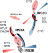 |
Fig. 9 Sketch of L1448N (expanded from Fig. 10 in Gieser et al. 2024). |
4.2 Kinematic properties from the envelope to disk scales
We have analyzed the kinematic properties of molecular gas from ≈36 000 au scales to 300 au. We found that the velocity profile of the two DCN streamers in IRS3A (Gieser et al. 2024) and the C18O streamer in IRS3C (Fig. 8, this work) agree with the large-scale rotation of the L1448N region (C18O 30m clusters 1 and 2 and C18O merged cluster 1 in Fig. 4) with blue- and redshifted velocities toward the west and east, respectively. This implies that these streamers are infalling structures that originate from the natal large-scale envelope material. The streamline model explicitly assumes that the particle trajectory originates from the larger-scale rotating envelope (Sect. 3.4). By using the combination of large-scale single-dish maps and sensitive NOEMA observations, we confirmed for the first time that this can be the case for observed streamers. When we compare our results with high-resolution ALMA observations resolving the disk rotation (Tobin et al. 2018; Reynolds et al. 2021), the rotational motion is coherent from the large-scale envelope to the infalling streamers and down to the disk scales. This implies that the protostellar systems have not formed in isolation, but originated from the same envelope material.
The SO2 streamer that falls onto IRS3C (which is also bright in SO emission; Fig. 3) does not follow the large-scale rotational pattern (Fig. 8), however. The emission of SO and SO2 is known to trace both accretion and ejection processes (Artur de la Villarmois et al. 2023), and SO is also prominent in the hot inner envelope (Tychoniec et al. 2021). Since the SO2 line width is not broadened (Fig. 4), the emission is likely not caused by a strong shock. It is more likely that the SO2 streamer is affected by the hotter inner region of IRS3C, and additional interactions with the outflow material might cause a change in the chemical composition with more abundant sulfur-bearing species. This streamer might originate from a cloudlet-capture event, as was proposed for the streamer in DG Tau (Hanawa et al. 2024). A case of three infalling streamers has been found toward the source IRAS 04239+2436 (Lee et al. 2023), where the spiral structures of the streamer were detected in SO emission, and one in addition in SO2. By comparing the observational results with magnetohydrodynamic simulations, the authors found that the streamers were consistent with gravitational interactions between the turbulent infalling envelope material and the central triple system and that the emission of S-bearing species originated from low-velocity shocks from these interactions. IRS3C is a binary system, so that this might also explain the SO2 streamer. The streamers traced by C18O and DCN in the region, on the other hand, are not bright in SO and SO2. This might imply a lower density and lower temperatures along these streamers, and shocks might therefore not play an important role. In contrast, the infall rate of the SO/SO2 streamer is higher. This might cause shocks through interaction with the envelope material, and potentially, even outflows.
The morphology of the large-scale IRAM 30 m map of SO is different from that of C18O (Fig. 2). These differences between molecular emission following the dust-continuum peak and molecular emission of SO and SO2 showing asymmetries with respect to the dust continuum can be evident already in the prestellar stage, as was observed toward the prestellar core L1544 (Spezzano et al. 2017). The SO2 streamer might originate from this gas reservoir. To investigate this potential connection, deep observations of sulfur-bearing species with a larger FOV are required.
5 Conclusions
We analyzed the kinematic properties of the L1448N region, which is located in the Perseus molecular cloud. To do this, we combined single-dish observations with the IRAM 30 m telescope (ANTIHEROES) and interferometric observations with NOEMA (PRODIGE) that trace scales from 36 000 to 300 au.
The C18O emission traces the large-scale envelope material in the single-dish maps, where we spectrally resolved large-scale rotation in which the three protostellar systems (IRS3A, IRS3B, and IRS3C) are embedded. The higher resolution of the combined data resolves highly substructured material.
Comparing NOEMA-only and merged (NOEMA+30m) C18O data, we found that more than 90% of the flux is filtered out in the interferometric data. With the exception of one SO2 transition, all other lines we analyzed were heavily affected by spatial filtering, with more than 50% missing flux. Not only the total flux, but also the line profiles are severely affected. The ANTIHEROES data therefore provide invaluable information of all molecular lines with extended emission of the entire PRODIGE sample.
Temperature maps using the c-C3H2 lines indicate a low temperatures (<20 K) on average in the region in the singledish and merged data. Higher temperatures are found in the merged data toward the location of the embedded protostars and toward the cavity walls of IRS3C.
Toward IRS3C, we found two infalling streamers that were detected in the C18O and sulfur-bearing species (SO, SO2). The velocity profiles and trajectories of the infalling streamers found toward IRS3C are consistent with gravitational infall.
The large-scale rotation of the L1448N envelope material traced by C18O (2 - 1) is coherent down to the streamer kinematics, as is the disk rotation of the three protostel-lar systems. The infalling streamers in C18O in IRS3C (this work) and DCN in IRS3A (Gieser et al. 2024) accelerate toward the protostellar systems. These infalling streamers are consistent with remnant envelope material that is carved out by the bipolar outflows. The SO2 streamer of IRS3C shows a different velocity pattern and might originate from an additional nearby gas reservoir that is detected in SO in the single-dish maps.
The infall rates of the streamers that fall onto IRS3A and IRS3C are 1 × 10⁻⁶ M⊙ yr-1 and 5-18 × 10-6 M⊙ yr-1, respectively. Thus, IRS3C, which is expected to be younger based on its bolometric temperature, accretes at higher accretion rates than IRS3A.
We found that streamers in young Class 0/I systems are connected to the remnant infalling envelope. In the same system, asymmetric gas inflows with an origin that is not consistent with the overall envelope motion can occur at the same time. The ongoing ANTIHEROES program for the first time enables a concise characterization of the origin and chemical composition of infalling material in order to better constrain the nature and impact of streamers in a sample of Class 0/I systems in the Perseus star-forming region. Further sensitive observations with a high angular resolution of molecular line tracers are then necessary to spatially resolve the connection to and effect of the infalling streamers on the disk properties.
Acknowledgements
The authors thank the anonymous referee for their constructive report that helped improve the clarity of this paper. The authors thank the IRAM staff at the NOEMA observatory and IRAM 30 m telescope for their support in the observations and data calibration. This work is based on observations carried out under project numbers L19MB and 096-23 with the IRAM NOEMA Interferometer and IRAM 30 m telescope, respectively. IRAM is supported by INSU/CNRS (France), MPG (Germany) and IGN (Spain). This project is co-funded by the European Union (ERC, SUL4LIFE, grant agreement No101096293). A.F. also thanks project PID2022-137980NB-I00 funded by the Spanish Ministry of Science and Innovation/State Agency of Research MCIN/AEI/10.13039/501100011033 and by “ERDF A way of making Europe”. D.S. has received funding from the European Research Council (ERC) under the European Union’s Horizon 2020 research and innovation programme (PROTOPLANETS, grant agreement No. 101002188).
References
- André, P., Di Francesco, J., Ward-Thompson, D., et al. 2014, in Protostars and Planets VI, eds. H. Beuther, R. S. Klessen, C. P. Dullemond, & T. Henning (Tucson: University of Arizona Press), 27–51 [Google Scholar]
- Artur de la Villarmois, E., Guzmán, V. V., Yang, Y. L., Zhang, Y., & Sakai, N. 2023, A&A, 678, A124 [NASA ADS] [CrossRef] [EDP Sciences] [Google Scholar]
- Ballesteros-Paredes, J., Hartmann, L. W., Pérez-Goytia, N., & Kuznetsova, A. 2015, MNRAS, 452, 566 [NASA ADS] [CrossRef] [Google Scholar]
- Busch, L. A., Pineda, J. E., Sipilä, O., et al. 2025, A&A, 699, A359 [NASA ADS] [CrossRef] [EDP Sciences] [Google Scholar]
- Cacciapuoti, L., Macias, E., Gupta, A., et al. 2024, A&A, 682, A61 [NASA ADS] [CrossRef] [EDP Sciences] [Google Scholar]
- Ceccarelli, C., Codella, C., Balucani, N., et al. 2023, ASP Conf. Ser., 534, 379 [NASA ADS] [Google Scholar]
- Chira, R. A., Kainulainen, J., Ibáñez-Mejía, J. C., Henning, T., & Mac Low, M. M. 2018, A&A, 610, A62 [NASA ADS] [CrossRef] [EDP Sciences] [Google Scholar]
- Ciardi, D. R., Telesco, C. M., Williams, J. P., et al. 2003, ApJ, 585, 392 [Google Scholar]
- Dunham, M. M., Stutz, A. M., Allen, L. E., et al. 2014, in Protostars and Planets VI, eds. H. Beuther, R. S. Klessen, C. P. Dullemond, & T. Henning (Tucson: University of Arizona Press), 195 [Google Scholar]
- Dunham, M. M., Stephens, I. W., Myers, P. C., et al. 2024, MNRAS, 533, 3828 [NASA ADS] [CrossRef] [Google Scholar]
- Enoch, M. L., Young, K. E., Glenn, J., et al. 2006, ApJ, 638, 293 [Google Scholar]
- Evans, Neal J. I., Dunham, M. M., Jørgensen, J. K., et al. 2009, ApJS, 181, 321 [NASA ADS] [CrossRef] [Google Scholar]
- Fernández-López, M., Girart, J. M., López-Vázquez, J. A., et al. 2023, ApJ, 956, 82 [CrossRef] [Google Scholar]
- Flores, C., Ohashi, N., Tobin, J. J., et al. 2023, ApJ, 958, 98 [NASA ADS] [CrossRef] [Google Scholar]
- Flores-Rivera, L., Terebey, S., Willacy, K., et al. 2021, ApJ, 908, 108 [NASA ADS] [CrossRef] [Google Scholar]
- Frerking, M. A., Langer, W. D., & Wilson, R. W. 1982, ApJ, 262, 590 [Google Scholar]
- Garufi, A., Podio, L., Codella, C., et al. 2022, A&A, 658, A104 [CrossRef] [EDP Sciences] [Google Scholar]
- Gerin, M., Pety, J., Commerçon, B., et al. 2017, A&A, 606, A35 [NASA ADS] [CrossRef] [EDP Sciences] [Google Scholar]
- Gieser, C., Pineda, J. E., Segura-Cox, D. M., et al. 2024, A&A, 692, A55 [NASA ADS] [CrossRef] [EDP Sciences] [Google Scholar]
- Ginsburg, A., Robitaille, T., Beaumont, C., et al. 2015, ASP Conf. Ser., 499, 363 [NASA ADS] [Google Scholar]
- Ginsburg, A., Sokolov, V., de Val-Borro, M., et al. 2022, AJ, 163, 291 [NASA ADS] [CrossRef] [Google Scholar]
- Ginski, C., Facchini, S., Huang, J., et al. 2021, ApJ, 908, L25 [NASA ADS] [CrossRef] [Google Scholar]
- Gupta, A., Miotello, A., Williams, J. P., et al. 2024, A&A, 683, A133 [NASA ADS] [CrossRef] [EDP Sciences] [Google Scholar]
- Hacar, A., Clark, S. E., Heitsch, F., et al. 2023, ASP Conf. Ser., 534, 153 [NASA ADS] [Google Scholar]
- Hanawa, T., Garufi, A., Podio, L., Codella, C., & Segura-Cox, D. 2024, MNRAS, 528, 6581 [NASA ADS] [CrossRef] [Google Scholar]
- Harju, J., Pineda, J. E., Vasyunin, A. I., et al. 2020, ApJ, 895, 101 [NASA ADS] [CrossRef] [Google Scholar]
- Högbom, J. A. 1974, A&AS, 15, 417 [Google Scholar]
- Hsieh, T. H., Segura-Cox, D. M., Pineda, J. E., et al. 2023, A&A, 669, A137 [NASA ADS] [CrossRef] [EDP Sciences] [Google Scholar]
- Hsieh, T. H., Pineda, J. E., Segura-Cox, D. M., et al. 2024, A&A, 686, A289 [NASA ADS] [CrossRef] [EDP Sciences] [Google Scholar]
- Kido, M., Takakuwa, S., Saigo, K., et al. 2023, ApJ, 953, 190 [NASA ADS] [CrossRef] [Google Scholar]
- Kido, M., Yen, H.-W., Sai, J., et al. 2025, ApJ, 985, 166 [Google Scholar]
- Kuffmeier, M. 2024, Front. Astron. Space Sci., 11, 1403075 [NASA ADS] [CrossRef] [Google Scholar]
- Kuffmeier, M., Calcutt, H., & Kristensen, L. E. 2019, A&A, 628, A112 [NASA ADS] [CrossRef] [EDP Sciences] [Google Scholar]
- Kuznetsova, A., Bae, J., Hartmann, L., & Mac Low, M.-M. 2022, ApJ, 928, 92 [NASA ADS] [CrossRef] [Google Scholar]
- Larson, R. B. 1969, MNRAS, 145, 271 [Google Scholar]
- Lattanzi, V., Bizzocchi, L., Vasyunin, A. I., et al. 2020, A&A, 633, A118 [NASA ADS] [CrossRef] [EDP Sciences] [Google Scholar]
- Lee, C.-F., Ho, P. T. P., Beuther, H., et al. 2006, ApJ, 639, 292 [Google Scholar]
- Lee, K. I., Dunham, M. M., Myers, P. C., et al. 2016, ApJ, 820, L2 [NASA ADS] [CrossRef] [Google Scholar]
- Lee, J.-E., Matsumoto, T., Kim, H.-J., et al. 2023, ApJ, 953, 82 [NASA ADS] [CrossRef] [Google Scholar]
- Looney, L. W., Lin, Z.-Y. D., Li, Z.-Y., et al. 2025, ApJ, 985, 148 [Google Scholar]
- Mangum, J. G., & Shirley, Y. L. 2015, PASP, 127, 266 [Google Scholar]
- Mendoza, S., Tejeda, E., & Nagel, E. 2009, MNRAS, 393, 579 [NASA ADS] [CrossRef] [Google Scholar]
- Mercimek, S., Podio, L., Codella, C., et al. 2023, MNRAS, 522, 2384 [NASA ADS] [CrossRef] [Google Scholar]
- Miotello, A., Kamp, I., Birnstiel, T., Cleeves, L. C., & Kataoka, A. 2023, ASP Conf. Ser., 534, 501 [NASA ADS] [Google Scholar]
- Miranzo-Pastor, J. J., Fuente, A., Navarro-Almaida, D., et al. 2025, A&A, 700, A251 [NASA ADS] [CrossRef] [EDP Sciences] [Google Scholar]
- Möller, T., Endres, C., & Schilke, P. 2017, A&A, 598, A7 [NASA ADS] [CrossRef] [EDP Sciences] [Google Scholar]
- Müller, H. S. P., Schlöder, F., Stutzki, J., & Winnewisser, G. 2005, J. Mol. Struc., 742, 215 [Google Scholar]
- Murillo, N. M., Fuchs, C. M., Harsono, D., et al. 2024, A&A, 689, A267 [NASA ADS] [CrossRef] [EDP Sciences] [Google Scholar]
- Offner, S. S. R., Kratter, K. M., Matzner, C. D., Krumholz, M. R., & Klein, R. I. 2010, ApJ, 725, 1485 [Google Scholar]
- Offner, S. S. R., Moe, M., Kratter, K. M., et al. 2023, ASP Conf. Ser., 534, 275 [NASA ADS] [Google Scholar]
- Pedregosa, F., Varoquaux, G., Gramfort, A., et al. 2011, J. Mach. Learn. Res., 12, 2825 [Google Scholar]
- Penston, M. V. 1969, MNRAS, 144, 425 [NASA ADS] [CrossRef] [Google Scholar]
- Pineda, J. E., Segura-Cox, D., Caselli, P., et al. 2020, Nat. Astron., 4, 1158 [NASA ADS] [CrossRef] [Google Scholar]
- Pineda, J. E., Arzoumanian, D., Andre, P., et al. 2023, ASP Conf. Ser., 534, 233 [NASA ADS] [Google Scholar]
- Podio, L., Ceccarelli, C., Codella, C., et al. 2024, A&A, 688, L22 [NASA ADS] [CrossRef] [EDP Sciences] [Google Scholar]
- Reynolds, N. K., Tobin, J. J., Sheehan, P., et al. 2021, ApJ, 907, L10 [NASA ADS] [CrossRef] [Google Scholar]
- Reynolds, N. K., Tobin, J. J., Sheehan, P. D., et al. 2024, ApJ, 963, 164 [Google Scholar]
- Ridge, N. A., Di Francesco, J., Kirk, H., et al. 2006, AJ, 131, 2921 [Google Scholar]
- Rodríguez-Baras, M., Fuente, A., Riviére-Marichalar, P., et al. 2021, A&A, 648, A120 [NASA ADS] [CrossRef] [EDP Sciences] [Google Scholar]
- Sakai, N., Sakai, T., Hirota, T., Burton, M., & Yamamoto, S. 2009, ApJ, 697, 769 [Google Scholar]
- Sakai, N., Sakai, T., Hirota, T., et al. 2014, Nature, 507, 78 [Google Scholar]
- Seifried, D., Banerjee, R., Pudritz, R. E., & Klessen, R. S. 2015, MNRAS, 446, 2776 [NASA ADS] [CrossRef] [Google Scholar]
- Shu, F. H. 1977, ApJ, 214, 488 [Google Scholar]
- Spezzano, S., Caselli, P., Bizzocchi, L., Giuliano, B. M., & Lattanzi, V. 2017, A&A, 606, A82 [NASA ADS] [CrossRef] [EDP Sciences] [Google Scholar]
- Steer, D. G., Dewdney, P. E., & Ito, M. R. 1984, A&A, 137, 159 [NASA ADS] [Google Scholar]
- Swade, D. A. 1989, ApJS, 71, 219 [Google Scholar]
- Tanious, M., Le Gal, R., Neri, R., et al. 2024, A&A, 687, A92 [NASA ADS] [CrossRef] [EDP Sciences] [Google Scholar]
- Tobin, J. J., Looney, L. W., Li, Z.-Y., et al. 2016, ApJ, 818, 73 [CrossRef] [Google Scholar]
- Tobin, J. J., Looney, L. W., Li, Z.-Y., et al. 2018, ApJ, 867, 43 [CrossRef] [Google Scholar]
- Tychoniec, Ł., van Dishoeck, E. F., van’t Hoff, M. L. R., et al. 2021, A&A, 655, A65 [NASA ADS] [CrossRef] [EDP Sciences] [Google Scholar]
- Valdivia-Mena, M. T., Pineda, J. E., Segura-Cox, D. M., et al. 2022, A&A, 667, A12 [NASA ADS] [CrossRef] [EDP Sciences] [Google Scholar]
- Valdivia-Mena, M. T., Pineda, J. E., Caselli, P., et al. 2024, A&A, 687, A71 [NASA ADS] [CrossRef] [EDP Sciences] [Google Scholar]
- van der Tak, F. F. S., Lique, F., Faure, A., Black, J. H., & van Dishoeck, E. F. 2020, Atoms, 8, 15 [Google Scholar]
- Vastel, C., Quénard, D., Le Gal, R., et al. 2018, MNRAS, 478, 5514 [Google Scholar]
- Volgenau, N. H., Mundy, L. G., Looney, L. W., & Welch, W. J. 2006, ApJ, 651, 301 [Google Scholar]
- Walch, S., Burkert, A., Whitworth, A., Naab, T., & Gritschneder, M. 2009, MNRAS, 400, 13 [NASA ADS] [CrossRef] [Google Scholar]
- Wilson, T. L., & Rood, R. 1994, ARA&A, 32, 191 [Google Scholar]
- Yen, H.-W., Takakuwa, S., Ohashi, N., et al. 2014, ApJ, 793, 1 [NASA ADS] [CrossRef] [Google Scholar]
- Yen, H.-W., Gu, P.-G., Hirano, N., et al. 2019, ApJ, 880, 69 [NASA ADS] [CrossRef] [Google Scholar]
- Zucker, C., Schlafly, E. F., Speagle, J. S., et al. 2018, ApJ, 869, 83 [NASA ADS] [CrossRef] [Google Scholar]
Appendix A Observation properties
Table A.1 summarizes the transition properties and observation parameters of all molecular lines analyzed in this work. The data calibration and imaging procedures are described in detail in Sect. 2.
Molecular line properties and observational parameters of the PRODIGE-ANTIHEROES data.
Appendix B Comparison of DCN (3 - 2) and C18O (2 - 1) NOEMA-only and merged data products
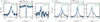 |
Fig. B.1 Spectra of DCN 3 - 2 (left) and C18O 2 - 1 (right) extracted from the continuum peak positions of IRS3A, IRS3B, and IRS3C. In black the NOEMA only spectrum is shown, while in blue the merged (NOEMA+30m) data are presented. The source vLSR is indicated by the vertical dashed line. |
Figure B.1 shows a comparison between DCN (3 - 2) and C18O (2 - 1) spectra extracted from the continuum peak positions of IRS3A, IRS3B and IRS3C using the NOEMA-only data and the merged data. Line-integrated intensity maps of both transitions comparing the single-dish, merged, and NOEMA-only data are shown in Fig. B.2.
The spatial distribution of DCN is mostly compact tracing the gas bridge toward IRS3A and IRS3B (Gieser et al. 2024), but the additional IRAM 30m short spacing information reveals weak extended emission around IRS3C. This extended emission surrounding IRS3C accounts for in total 57% missing flux in DCN (3 - 2) considering all areas with emission > 5σ in the line-integrated intensity maps (Fig. B.2). The kinematic properties of the gas bridge analyzed in Gieser et al. (2024) using the DCN (3 - 2) transition is not affected by spatial filtering with similar intensities measured in the merged and NOEMA data toward IRS3A and IRS3B.
The emission of C18O (2 - 1) however is very extended being detected in the entire single-dish map. Comparing the merged and NOEMA-only integrated intensity maps stresses that while compact structures are recovered by NOEMA, most of the extended emission is not. In the C18O (2 - 1) NOEMA data the missing flux is in total 93%. While the integrated intensity maps of the NOEMA data have large areas with negative values, adding additional 30m data removes these artifacts completely.
In Table A.1 the percentage of missing flux is summarized for all transitions with extended emission used in this work. The amount of missing flux depends heavily on the transition and varies between 57% and 98%. Both the total flux Fig. B.2) and velocity profiles (Fig. B.1) of the C18O (2 - 1) are different in the merged and NOEMA-only data. Hence, the NOEMA-only data should not be used in the case of molecular emission with extended emission when the analysis relies total flux measurements and/or kinematic properties.
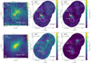 |
Fig. B.2 Line-integrated intensity map of DCN (3 - 2) and C18O (2 - 1) of the IRAM 30m data (left) and merged data (center), and NOEMA data (right). Red contours highlight emission of -5σ (dotted) and 5σ (solid). If no contours are shown, the emission is > 5σ in the entire FOV. Pink contours and arrows are the same as in Fig. 1. The synthesized beam of the line and continuum data is shown in the bottom left and right corner, respectively. Scale bars are shown in the top left corner. |
Appendix C Details of the kinematic analysis
Overview of the kinematic analysis.
Figure C.1 shows spectra extracted from IRS3A, IRS3B, and IRS3C continuum peak positions comparing the line profiles of DCN (3 - 2), c-C3H2 (60,6 - 51,5), C18O (2 - 1), SO (65 — 54), and SO2 (42,2 - 31,3). The strong line absorption of DCN and C18O toward IRS3B is due to absorption against the bright continuum background emission. The high spectral resolution of the molecular line data allows a detailed analysis of the kinematic properties of the gas conducted in Sect. 3.1. Here, a detailed description of the methodology based on the analysis of IRS3A (Gieser et al. 2024) is presented.
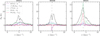 |
Fig. C.1 Molecular line spectra extracted from the continuum peak positions of IRS3A (left), IRS3B (center), and IRS3C (right). The source vLSR is indicated by the vertical dashed line. For SO2 the NOEMA-only data, while for the remaining transitions the merged (NOEMA+IRAM 30m) data is shown (Table A.1). |
In Sect. 3.1 we perform a Gaussian decomposition of C18O (2-1) and SO2 (42,2 - 31,3) where up to three velocity components are fitted in each spectrum. Given the increase of noise toward the edges of the FOV, the noise (per 0.1 km s-1 channel) is estimated in each spectrum individually. The minimum amplitude of each Gaussian velocity component is set to at least 5× the noise and the minimum full-width at half maximum (FWHM) line width is set to 0.1 km s-1 . We discard all pixels with a defined maximum noise value σline,max to mask noisy areas at the edges of the FOV.
We evaluate the goodness of the one-, two-, and three-component fits in each spectrum based on the Akaike Information Criterion (AIC). The best-fit is selected based on the lowest AIC value, but only if the difference to the second lowest value is higher than ∆AIC, defined for each transition. We perform a second quality assessment where we discard all velocity components which have relative uncertainties in any of the fit parameters (peak velocity v, FWHM line width ∆v, amplitude Ipeak) higher than a defined percentage. The quality assessment of the fitted Gaussian velocity components is summarized in Table C.1 for all analyzed datasets.
Given the extended emission and complex spectral line profiles of C18O in both the single-dish and merged data, our criteria are more conservative compared to SO2, in order to only extract the most reliable velocity components. We note that in the C18O merged data due to our conservative approach many velocity components are discarded after the quality assessment, even though line emission may be bright, but in many cases line profiles are too complex to fit them properly. This is especially the case toward the complex bridge region surrounding IRS3A and IRS3B where in addition to the infalling gas bridge, there is a significant contribution from outflows and rotation of the compact envelopes and disks (Fig. C.1).
The dataset with up to three velocity components per spectrum is sorted using the clustering algorithm DBSCAN. The clustering in DBSCAN is set by two parameters, the neighborhood parameter eps (ε) and the minimum number of data points within a cluster minsamples. For all datasets we check the parameter space of these two parameters and find a combination of the two that 1) creates smooth velocity maps in each cluster that also produce coherent amplitude and line width maps, 2) has a low number of discarded points, 3) is able to disentangle the velocity components at a certain position, so averaging of the data points within a single pixel is minimized. The input parameters and clustering results are summarized in Table C.1. Additional clusters as well as the discarded data points extracted with DBSCAN in Sect. 3.1 are summarized in Fig. C.2.
For example, large-scale redshifted emission in C18O single-dish data (C18O (IRAM 30m) cluster 3) is most likely connected to a background cloud component because there is no known outflow in this direction. The disk rotation of IRS3C is extracted in SO2 (NOEMA) cluster 2. The redshifted SO2 blob (SO2 (NOEMA) cluster 3) toward the northwest might be connected to the arc structure (SO2 (NOEMA) cluster 1), that is, the arc is wrapping around behind the source where it is infalling. In the merged C18O dataset, many redshifted blobs are extracted in four clusters, oriented along the redshifted outflow lobe launched by IRS3C (C18O (merged) clusters 3, 4, 7, and 8). Blueshifted outflow components are seen as well for IRS3B (C18O (merged) cluster 2) and IRS3C (C18O (merged) cluster 9).
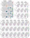 |
Fig. C.2 The same as Fig. 4 presenting the main clusters, while here remaining clusters extracted with DBSCAN are shown. |
Appendix D Excitation conditions of c-C3H2
Integrated intensity maps of all three detected c-C3 H2 transitions are shown in Fig. D.1. In Sect. 3.2 we use the XCLASS tool to derive the rotation temperature and column density maps. The detailed setup of the line fitting with XCLASS is described in the following.
Since the noise is not homogeneous and in general increases toward the edges of the FOV, we evaluate the noise in each pixel individually. The noise is computed from the average noise calculated in line-free velocity ranges on the blue- and redshifted sides of each emission line. All pixels with noise values higher than 0.15 K and 0.4 K in the 30m and merged data, respectively, are flagged which correspond to areas at the edge of the FOV. We then compute S/N maps of all transitions and only spectra where the S/N is larger than 6 for all three transitions are fitted with XCLASS.
The myXCLASSFit function solves the radiative transfer equation of an isothermal source for all selected transitions of a molecule assuming local thermal equilibrium (LTE) conditions. The critical densities for the three c-C3H2 transitions range between 4 - 5 × 107 cm-2 (using collisional rates at 30 K from the Leiden Atomic and Molecular Database, van der Tak et al. 2020). In a spherical symmetric envelope approximation, at distances of several hundreds of au from the protostar, densities can reach such high densities (Gerin et al. 2017). At larger distances, the underlying kinetic temperature might be slightly underestimated from this approach. The fit parameter set includes the source size θsource, rotation temperature Trot, column density N, FWHM line width ∆v, and peak velocity v.
To reduce the fit parameter set, we fix the source size θsource to 12″ and 2″ for all 30 m and merged data, respectively. This implies a beam filling factor of 1, which is reasonable since the emission is extended for all c-C3H2 transitions (Fig. D.1). The best-fit model (based on the lowest reduced χ2) is determined by using an algorithm chain starting with the Genetic algorithm (100 iterations) followed by the Levenberg-Marquart algorithm (50 iterations) optimizing the parameter set toward global and local minima, respectively.
Appendix E Column density maps of the envelope and the streamers
Column density maps of the L1448N envelope and the streamers infalling onto IRS3A and IRS3C are presented in Fig. E.1 and are used to estimate the masses in Sect. 3.5.
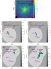 |
Fig. E.1 Column density maps of the L1448N and the streamers. Contours and arrows are the same as in Fig. 1. The synthesized beam of the line and continuum data is shown in the bottom left and right, respectively. A scale bar is indicated in the top left corner. The IRS3A DCN streamers were analyzed in Gieser et al. (2024) and IRS3C C18O and SO2 streamers were analyzed in this work. |
CLIC, CLASS, and MAPPING are software from the standard observatory pipeline in the Grenoble Image and Line Data Analysis Software (GILDAS, https://www.iram.fr/IRAMFR/GILDAS/).
All Tables
Molecular line properties and observational parameters of the PRODIGE-ANTIHEROES data.
All Figures
|
Fig. 1 Continuum images toward L1448N. The left panel shows large-scale 1.1 mm continuum emission of L1448 (Enoch et al. 2006). The beam size is shown in the bottom left corner. The map size of the IRAM 30 m observations is highlighted by the dashed gray rectangle. The right panel shows the NOEMA 1.4 mm continuum of L1448N with contour levels at 5, 25, 60, 120, 200 times σcont with σcont = 0.78 mJy beam-1. The triangles and white labels mark the positions of individual protostars (Tobin et al. 2016), and the pink cross marks the recently detected source IRS3-ALMA (Looney et al. 2025). The bipolar outflow directions launched by the three protostellar systems are marked by red and blue arrows, including the blueshifted outflow lobe that is launched by L1448-mm toward the southeast. The synthesized beam of the NOEMA continuum data is shown in the bottom left corner. The scale bars in the two panels are shown in the top left corner. |
| In the text | |
|
Fig. 2 Line-integrated intensity map of C18O (2 - 1), SO (65 - 54), and SO2 (42,2 - 31,3) of the IRAM 30 m data (left) and merged or NOEMA data (right). The line-integrated intensity is shown in color in all panels. The contours and arrows are the same as in Fig. 1. The synthesized beam of the line and continuum data is shown in the bottom left and right corners, respectively. The scale bars are shown in the top left corner in all panels. In the right panels, distinct structures (bridge and stick) seen in molecular emission are indicated by dashed ellipses. |
| In the text | |
|
Fig. 3 Channel maps of SO 65 - 54 (top, merged data) and SO2 42,2 - 31,3 (bottom, NOEMA-only data) toward L1448 IRS3C. The green color map shows the line intensity with the velocity of the channel in km s-1 labeled in the bottom right. The black contours are the same as in Fig. 1. The dashed red and solid blue contours indicate the CO (2 - 1) integrated intensity of the red- and blueshifted outflow launched by IRS3C. The integration ranges are 5.9-27 km s-1 and 2-3.4 km s-1 (narrow range to avoid foreground contamination) with contour levels at 0.1, 0.3, 0.5, and 0.7 and 0.5, 0.7, and 0.9 times the peak-integrated intensity, respectively. In the top left panel, the black scale bar in the top right corner indicates a spatial scale of 1 000 au. The synthesized beam of the line and continuum data are shown in the bottom left and right corners, respectively. In each panel, the scale is set from a minimum brightness temperature of -0.3 K to a maximum of 7 K. The IRS3C source velocity is 3.8 km -1 (Sect. 3.3). |
| In the text | |
|
Fig. 4 Main clusters extracted with DBSCAN. The velocity, peak intensity, and line width are shown in color in the top, central, and bottom panels, respectively. The contours and arrows are the NOEMA 1.4 mm continuum with the same levels as in Fig. 1. In cluster 1 of each analyzed dataset, the synthesized beam of the line and continuum data is shown in the bottom left and right corner, respectively, and scale bars are shown in the top left corner. The remaining clusters are shown in Fig. C.2. |
| In the text | |
|
Fig. 5 Parameter maps of c-C3 H2 (rotation temperature, column density, FWHM line width, and peak velocity) of the IRAM 30 m (left) and merged (right) data. The contours and arrows are the same as in Fig. 1. The beams of the line and continuum data are shown in the bottom left and right corners, respectively. The scale bars are indicated in the top left corner. |
| In the text | |
|
Fig. 6 Spectrum of DCN (3 - 2) extracted from the IRS3C continuum peak position The observed spectrum is shown in black, and a two-Gaussian velocity componen fi s hown in bue and red. The dashed purple line marks the 3σline level. The source velocity estimated from the red componen is indicated by the vertical dashed line. |
| In the text | |
|
Fig. 7 Position velocity diagram of SO2 (42,2 - 31,3) extracted along the disk orientation of IRS3C. The black contours show the 4, 8, and 16σline levels. The red line shows the profile for a Keplerian disk of 1 M⊙ inclined by 50°, and for comparison, the dotted cyan and green lines show profiles for 0.5 M⊙ and 2 M⊙, respectively. A spectral and spatial resolution element (0.1 km s-1 ×283 au) is indicated in the bottom left corner. |
| In the text | |
|
Fig. 8 Streamline models toward IRS3C. In the left panels, the line-integrated intensity and the velocities of the structure are shown in gray and color, respectively. The trajectory of the best-match streamline model is shown in green. The contours are the NOEMA 1.4 mm continuum with the same levels as in Fig. 1. The beam of the line and continuum data are shown in the bottom left and right corners, respectively. A scale bar is shown in the top right corner. In the right panels, we indicate the velocity distribution extracted from the areas by dotted ellipses (left) in red or blue, and the best-match streamline model is shown in green. The source velocity of IRS3C (3.8 km s-1) is indicated by the horizontal dashed line. |
| In the text | |
|
Fig. 9 Sketch of L1448N (expanded from Fig. 10 in Gieser et al. 2024). |
| In the text | |
|
Fig. B.1 Spectra of DCN 3 - 2 (left) and C18O 2 - 1 (right) extracted from the continuum peak positions of IRS3A, IRS3B, and IRS3C. In black the NOEMA only spectrum is shown, while in blue the merged (NOEMA+30m) data are presented. The source vLSR is indicated by the vertical dashed line. |
| In the text | |
|
Fig. B.2 Line-integrated intensity map of DCN (3 - 2) and C18O (2 - 1) of the IRAM 30m data (left) and merged data (center), and NOEMA data (right). Red contours highlight emission of -5σ (dotted) and 5σ (solid). If no contours are shown, the emission is > 5σ in the entire FOV. Pink contours and arrows are the same as in Fig. 1. The synthesized beam of the line and continuum data is shown in the bottom left and right corner, respectively. Scale bars are shown in the top left corner. |
| In the text | |
|
Fig. C.1 Molecular line spectra extracted from the continuum peak positions of IRS3A (left), IRS3B (center), and IRS3C (right). The source vLSR is indicated by the vertical dashed line. For SO2 the NOEMA-only data, while for the remaining transitions the merged (NOEMA+IRAM 30m) data is shown (Table A.1). |
| In the text | |
|
Fig. C.2 The same as Fig. 4 presenting the main clusters, while here remaining clusters extracted with DBSCAN are shown. |
| In the text | |
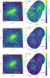 |
Fig. D.1 Same as Fig. 2, but for the c-C3 H2 transitions. |
| In the text | |
|
Fig. E.1 Column density maps of the L1448N and the streamers. Contours and arrows are the same as in Fig. 1. The synthesized beam of the line and continuum data is shown in the bottom left and right, respectively. A scale bar is indicated in the top left corner. The IRS3A DCN streamers were analyzed in Gieser et al. (2024) and IRS3C C18O and SO2 streamers were analyzed in this work. |
| In the text | |
Current usage metrics show cumulative count of Article Views (full-text article views including HTML views, PDF and ePub downloads, according to the available data) and Abstracts Views on Vision4Press platform.
Data correspond to usage on the plateform after 2015. The current usage metrics is available 48-96 hours after online publication and is updated daily on week days.
Initial download of the metrics may take a while.