| Issue |
A&A
Volume 701, September 2025
|
|
|---|---|---|
| Article Number | A261 | |
| Number of page(s) | 15 | |
| Section | Planets, planetary systems, and small bodies | |
| DOI | https://doi.org/10.1051/0004-6361/202555702 | |
| Published online | 25 September 2025 | |
The GAPS Programme at TNG
LXIX. The dayside of WASP-76 b revealed by GIANO-B, HARPS-N, and ESPRESSO: Evidence of 3D atmospheric effects★
1
INAF – Osservatorio Astrofisico di Torino,
Via Osservatorio 20,
10025
Pino Torinese,
Italy
2
Department of Physics, University of Turin,
Via Pietro Giuria 1,
10125
Torino,
Italy
3
INAF – Osservatorio Astronomico di Brera,
Via E. Bianchi 46,
23807
Merate,
Italy
4
Institut Trottier de Recherche sur les Exoplanètes, Université de Montréal,
Montréal,
Québec
H3T 1J4,
Canada
5
Dipartimento di Fisica e Astronomia “Galileo Galilei”, Università di Padova,
Vicolo dell’Osservatorio 3,
35122
Padova,
Italy
6
Space Research Institute, Austrian Academy of Sciences,
Schmiedl-strasse 6,
8042
Graz,
Austria
7
INAF – Osservatorio Astrofisico di Arcetri,
Largo E. Fermi 5,
50125
Firenze,
Italy
8
INAF – Osservatorio Astronomico di Trieste,
via Tiepolo 11,
34143
Trieste,
Italy
9
INAF – Osservatorio Astronomico di Palermo,
Piazza del Parlamento, 1,
90134
Palermo,
Italy
10
Fundación Galileo Galilei-INAF,
Rambla José Ana Fernandez Pérez 7,
38712
Breña Baja,
TF,
Spain
11
Department of Physics, University of Rome “Tor Vergata”,
Via della Ricerca Scientifica 1,
00133
Roma,
Italy
12
Max Planck Institute for Astronomy,
Königstuhl 17,
69117
Heidelberg,
Germany
13
INAF – Osservatorio Astronomico di Padova,
Vicolo dell’Osservatorio 5,
35122
Padova,
Italy
14
Centro di Ateneo di Studi e Attività Spaziali “G. Colombo” – Università degli Studi di Padova,
Via Venezia 15,
35131
Padova,
Italy
15
INAF – Osservatorio Astrofisico di Catania,
Via S. Sofia 78,
95123
Catania,
Italy
★★ Corresponding author: This email address is being protected from spambots. You need JavaScript enabled to view it.
Received:
28
May
2025
Accepted:
24
July
2025
Abstract
Context. The study of the atmosphere of ultra-hot Jupiters (UHJs) with equilibrium temperatures ≥2000 K provides valuable insights into atmospheric physics under such extreme conditions.
Aims. We aim to characterise the dayside thermal spectrum of the UHJ WASP-76 b and investigate its properties. We analysed data gathered with three high-resolution spectrographs: specifically two nights with simultaneous observations of HARPS-N and GIANO-B, and four nights of publicly available ESPRESSO optical spectra. We observed the planet’s dayside, covering orbital phases between quadratures (0.25 < ϕ < 0.75).
Methods. We performed a homogeneous analysis of the GIANO-B, HARPS-N, and ESPRESSO data and co-added the signal of thousands of planetary lines through cross-correlation with simulated spectra of the planetary atmosphere.
Results. We report the detection of CO in the dayside atmosphere of WASP-76 b with a signal-to-noise ratio (S/N) of 10.4 in the GIANO-B spectra. In addition, we detect Fe I in both the HARPS-N and ESPRESSO datasets, with S/N values of 3.5 and 6.2, respectively. A signal from Fe I is also identified in one of the two GIANO-B observations, with an S/N of 4.0. Interestingly, a qualitatively similar pattern – with a weaker detection in one epoch compared to the other – is also observed in the two HARPS-N nights. The GIANO-B results are, therefore, consistent with those obtained with HARPS-N. Finally, we compared our strongest detections of CO (GIANO-B) and Fe I (ESPRESSO), with predictions from global circulation models (GCM). Both cross-correlation and likelihood analyses favour the GCM that includes atmospheric dynamics over a static (no-dynamics) model when applied to the ESPRESSO data. This study adds to the growing body of literature employing GCMs to interpret high-resolution spectroscopic measurements of exoplanet atmospheres.
Key words: methods: observational / techniques: spectroscopic / planets and satellites: atmospheres
Based on observations made with the Italian Telescopio Nazionale Galileo (TNG) operated on the island of La Palma by the Fundacion Galileo Galilei of the INAF at the Spanish Observatorio Roque de los Muchachos of the IAC in the frame of the program Global Architecture of the Planetary Systems (GAPS).
© The Authors 2025
 Open Access article, published by EDP Sciences, under the terms of the Creative Commons Attribution License (https://creativecommons.org/licenses/by/4.0), which permits unrestricted use, distribution, and reproduction in any medium, provided the original work is properly cited.
This article is published in open access under the Subscribe to Open model. This email address is being protected from spambots. You need JavaScript enabled to view it. to support open access publication.
1 Introduction
Over the past 20 years, the characterisation of exoplanetary atmospheres has established itself as a fundamental and rapidly evolving research area in the field of exoplanets. From an observational perspective, high-resolution spectroscopy (HRS) using ground-based observatories, with current resolving powers ranging from R = 25 000 to 140 000, has proven to be a powerful technique for studying and characterising exoplanetary atmospheres (see the reviews by Birkby 2018; Brogi & Birkby 2021 and references therein). This observational technique allows us to: (i) resolve molecular bands and atomic lines into individual spectral lines, enabling a better identification of different chemical components, and (ii) exploit the Doppler shift of the planet’s spectrum to disentangle it from both the Earth’s atmospheric transmission and the host star’s spectrum, and thus enabling the determination of the planet’s atmospheric circulation (e.g. Ehrenreich et al. 2020; Seidel et al. 2020, 2021; Pino et al. 2022; Seidel et al. 2025).
Using HRS, various chemical species have been detected in exoplanetary atmospheres across both visible and near-infrared (nIR) bands (e.g. Snellen et al. 2010; Brogi et al. 2012; Birkby et al. 2013; Wyttenbach et al. 2015; Hoeijmakers et al. 2019; Giacobbe et al. 2021; Pelletier et al. 2023). Atmospheric dynamics, such as winds and global circulation patterns, have also been observed (e.g. Brogi et al. 2016; Louden & Wheatley 2015; Ehrenreich et al. 2020; Kesseli & Snellen 2021; Seidel et al. 2025).
Simultaneously, theoretical models have become increasingly sophisticated, enabling the testing of more complex planetary scenarios. Global circulation models (GCMs), which are 3D numerical simulations of atmospheric dynamics, now provide critical tools for detailed atmospheric studies (e.g. Showman et al. 2013; Rauscher & Kempton 2014). Originally developed for Earth’s climate studies, GCMs have been adapted to simulate exoplanet atmospheres, particularly for tidally locked hot Jupiters orbiting close to their stars. These models solve the equations of fluid dynamics and radiative transfer, capturing 3D variations in temperature, winds, and chemical composition across the planet. By accounting for spatial and temporal variations, such as day-night contrasts and equatorial jets, GCMs offer a consistent physical framework for interpreting observations such as phase curves, emission, and transmission spectra. In particular, they reveal how atmospheric circulation influences the shape and position of spectral lines, providing a more realistic alternative to traditional 1D models for high-resolution spectroscopy (Showman et al. 2010).
Ultra-hot Jupiters (UHJs), which orbit extremely close to their host stars (Porb ≲ 3 days for a main-sequence star), are exposed to intense stellar irradiation, resulting in equilibrium temperatures that can exceed 2000 K. These extreme conditions make UHJs ideal laboratories for studying atmospheric physics in regimes that are inaccessible within the Solar System. There is growing evidence that UHJs exhibit atmospheric properties that differ significantly from those of cooler hot Jupiters. At temperatures above ∼2000 K, molecules start to thermally dissociate and atoms ionise (e.g. Arcangeli et al. 2018; Parmentier et al. 2018). At these high temperatures, H− becomes a dominant source of opacity and significantly shapes the emergent spectrum (e.g. Gandhi et al. 2020). Furthermore, it has been shown that the hotter the planet’s equilibrium temperature, the more likely it is to exhibit a thermal inversion in its atmosphere (e.g. Baxter et al. 2020). As a result, UHJs may transition from a non-inverted to an inverted atmospheric structure as temperatures increase. UHJs thus offer a unique opportunity to test and refine GCMs.
Several UHJs have been extensively investigated in the literature (see, e.g. Stangret et al. 2024 and references therein) through both transmission and emission spectroscopy, utilising spectrographs mounted on both ground-based high-resolution and space-borne low-resolution instruments.
WASP-76 b (Mp=0.894 MJup, Rp=1.854 RJup) is a shortperiod (P = 1.81 d) UHJ orbiting the bright F7 main sequence star WASP-76 A (Teff = 6329 ± 65 K, V = 9.52, K = 8.243). The parameters for WASP-76 b and its host star are listed in Table 1. The equilibrium temperature of WASP-76 b is approximately ∼2228 K (Ehrenreich et al. 2020); however, due to its tidal locking, the dayside temperature can exceed ∼3000 K (e.g. Garhart et al. 2020; Wardenier et al. 2025). Thermal inversion layers are known to exist on the dayside of this planet, such that temperature increases with altitude (e.g. Edwards et al. 2020; Yan et al. 2023; Costa Silva et al. 2024).
WASP-76 b is a reference UHJ that has been extensively studied. Numerous atomic, ionised, and molecular species have been identified in its atmosphere at HRS (Seidel et al. 2019; Ehrenreich et al. 2020; Casasayas-Barris et al. 2021; Deibert et al. 2021; Kesseli & Snellen 2021; Landman et al. 2021; Tabernero et al. 2021; Wardenier et al. 2021; Azevedo Silva et al. 2022; Gandhi et al. 2022; Kawauchi et al. 2022; Kesseli et al. 2022; Sánchez-López et al. 2022; Savel et al. 2022; Deibert et al. 2023; Gandhi et al. 2023; Wardenier et al. 2023; Yan et al. 2023; Pelletier et al. 2023; Maguire et al. 2024; Masson et al. 2024; Weiner Mansfield et al. 2024; Costa Silva et al. 2024). A comprehensive reference for all studies of this planet is given in Table 2 of Costa Silva et al. (2024).
However, most of these studies have relied on 1D atmospheric models for comparison. Yet, the atmosphere of WASP-76 b is inherently 3D and, by relying only on 1D approaches, we risk overlooking critical signatures of this 3D nature. As recently emphasised by Wardenier et al. (2025), the 3D thermal structure of the planet exerts an even stronger influence on the emission line profiles than on those observed in transmission. In transmission spectroscopy, line depths are determined by altitude differences between the line core and the continuum pressure levels. In emission, however, the line contrast depends directly on the difference in thermal flux between these atmospheric layers. If the temperature increases with altitude (as in a thermal inversion), this results in emission lines; otherwise, absorption lines are expected. Since emission spectra integrate flux from the entire planetary disk, sampling both hotter dayside and cooler nightside regions, the resulting line shapes reflect a range of vertical temperature structures that cannot easily be captured by 1D models (Beltz et al. 2021). Additionally, 3D GCMs predict that emission-line Doppler shifts vary with the orbital phase, potentially explaining observed offsets in Kp versus Vrest maps (Wardenier et al. 2025). The interplay between tidally locked rotation and spatial temperature variations may also cause emission line strengths to change throughout the orbit. Such effects have already been reported in UHJ emission studies, where cross-correlation (CC) signals for species such as Fe and CO exhibit unexpected significant velocity changes between pre- and post-eclipse observations. For WASP-76 b, Costa Silva et al. (2024) do not detect a Kp offset for Fe I in the pre- and post-eclipse spectra obtained with the Echelle SPectrograph for Rocky Exoplanets and Stable Spectroscopic Observations (ESPRESSO), but report a blueshift along the υsys axis of −4.7 ± 0.3 km s−1 (we discuss this result further in Sect. 4). In contrast, Yan et al. (2023) report negative Kp offsets for CO, although with large uncertainties (Kp =  km s−1).
Motivated by these findings, we collected new GIARPS (GIANO-B + HARPS-N) data and analysed them (see Sect. 2 for further details) in combination with publicly available ESPRESSO spectra. Our goal is to analyse the dayside of WASP-76 b through the detection of Fe I and CO and to assess the impact of atmospheric dynamics on the observed high-resolution spectra, by studying the 3D structure of WASP-76 b’s atmosphere. Emission lines from CO and Fe I have been widely used to investigate temperature inversions in UHJs (e.g. Pino et al. 2020; Yan et al. 2020; Borsa et al. 2022; Yan et al. 2022), offering valuable insight into the thermal structure of their atmospheres. Because of its high thermal dissociation temperature, CO is especially well suited to trace the hottest regions of the dayside in these extreme environments. In particular, CO and Fe I have been detected on the dayside of WASP-76 b by Yan et al. (2023) and Costa Silva et al. (2024), respectively.
This paper is organised as follows. We describe the observations in Sect. 2 and detail the data reduction procedures in Sect. 3. We highlight our findings in Sect. 4. Finally, we discuss our results and present our conclusions in Sect. 5.
2 Observations
We analysed two dayside emission observations of WASP-76 b (2023-10-11 and 2023-11-15; hereafter N1 and N2) gathered with the GIARPS observing mode of the Telescopio Nazionale Galileo (TNG; Claudi et al. 2017) as part of the Building a Road to the In-Depth investiGation of Exoplanetary atmosphereS (BRIDGES) programme (PI F. Borsa) within the Global Architecture of Planetary Systems (GAPS) Collaboration (Covino et al. 2013). We also re-analysed four ESPRESSO datasets (202109-02, 2021-09-09, 2022-10-14, and 2022-10-18; hereafter N3, N4, N5, and N6), which we downloaded from the ESO public archive. The data were obtained as part of programmes 1104.C-0350(U) and 110.24CD.004 of the Guaranteed Time Observations.
In this section, we describe the GIARPS observations and refer the reader to Costa Silva et al. (2024) for further details on the ESPRESSO dataset.
When observing in GIARPS mode, the TNG can simultaneously acquire high-resolution spectra in the optical range (0.39– 0.69 µm) and nIR range (0.95–2.45 µm) using the HARPS-N (R ≈ 115 000) and GIANO-B (R ≈ 50 000) spectrographs. For the GIANO-B observations, we employed an ABAB nodding pattern, which allows for optimal subtraction of thermal background noise and telluric emission lines. The GIANO-B spectrograph covers four spectral bands in the nIR (Y, J, H, K), divided into 50 orders. A detailed log of the GIARPS observations is provided in Table 2. Figure 1 shows the average (S/N) in the GIANO-B spectra as a function of the planet’s orbital phase and airmass for each night considered.
The HARPS-N observations were carried out with fibre B placed on the sky. HARPS-N covers 69 different orders for each fibre, using an echelle spectrograph design.
Properties of the planet WASP-76 b and its stellar host.
Observations log.
3 Data analysis
In this work, we fully exploited the capabilities of the GIARPS instrument by analysing data from both GIANO-B and HARPS-N, and complemented these with archival observations from ESPRESSO. Our goal was to maintain a consistent approach across the different datasets, focussing on the detection of CO and Fe I in the dayside of WASP-76 b.
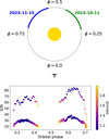 |
Fig. 1 Top panel: schematic representation of the orbit of WASP-76 b. The orbital phases covered in this study with GIARPS are colour-coded according to observing night. Bottom panel: S/N averaged over orders as a function of the orbital phase for nights in emission. The markers’ colour is proportional to the airmass. The exposures with higher S/N are from HARPS-N, while those with lower S/N are from GIANO-B. |
3.1 Data reduction and calibration
We processed the raw GIANO-B spectra using the GOFIO pipeline (Rainer et al. 2018), which performs flat-fielding, bad-pixel correction, background subtraction, optimal extraction of the 1D spectra, and an initial wavelength calibration based on a uranium-neon lamp. To account for small temporal variations in the wavelength solution – typically derived at the end of the night and potentially affected by instrumental instabilities during observations (Giacobbe et al. 2021) – we corrected and refined the solution. Specifically, we aligned all spectra from a given night to a common reference frame by cross-correlating each exposure with the time-averaged observed spectrum of the target, which served as a template. We then exploited the stationarity of telluric lines to further refine the wavelength calibration. In particular, after aligning the spectra, we performed a more accurate wavelength calibration by matching a set of telluric features in the time-averaged spectrum to a high-resolution transmission spectrum of the Earth’s atmosphere, generated with the ESO Sky Model Calculator1. However, due to the presence of spectral regions with either too many or too few telluric lines, it was not possible to apply this calibration refinement to all spectral orders (e.g. Brogi et al. 2018; Guilluy et al. 2022; Carleo et al. 2022; Basilicata et al. 2024). We therefore excluded a set of spectral orders heavily affected by telluric contamination (orders 8–10 and 23–25), the Y-band region (orders 40–49), where GIANO-B exhibits a significant drop in throughput, and approximately 10 additional orders (depending on the night) due to high residual drift or failures in the refined wavelength calibration procedure.
For the HARPS-N observations, we calibrated the data using standard data reduction software (DRS v3.7.1; Cosentino et al. 2012) and extracted the ED2S files. The ESPRESSO spectra were reduced with the dedicated pipeline (DRS v3.2.5) provided by ESO and the ESPRESSO Consortium (Pepe et al. 2021). For our analysis, we used the S2D spectra, which are referenced to the barycentric rest frame of the Solar System. In contrast, the GIARPS spectra are provided in the telluric rest frame.
For HARPS-N, we converted the wavelength calibration from air to vacuum using the values retrieved from the file headers to ensure consistency with the wavelength solutions of GIANO-B and ESPRESSO. No further realignment or wavelength correction was applied to either HARPS-N or ESPRESSO data, given the high intrinsic stability of both spectrographs.
3.2 Telluric and stellar removal
We removed the telluric contamination by employing principal component analysis (PCA; Giacobbe et al. 2021) with the spectra aligned in the Earth’s rest frame. Before applying PCA, we performed some preliminary steps (Basilicata et al. 2024). Specifically, after converting the spectra into logarithmic space, we corrected for baseline flux variations by normalising each spectrum to its median value. We then identified and masked spectral channels contaminated by strong or saturated telluric lines using the same procedure adopted in Basilicata et al. (2024). Next, we computed the standard deviation of each spectral channel and its median value σm (after subtracting, for each pixel, the mean flux across the time axis, i.e. over all images) and masked pixels with variability exceeding a threshold defined as 1.5×σm (Basilicata et al. 2024). The positions of these masked pixels were recorded and excluded from further analysis. This step ensured that highly variable or defective pixels did not bias the PCA decomposition, improving the robustness of the extracted components. After subtracting the time-averaged spectrum from all spectra, we subtracted the mean value of each spectrum, computed across its spectral channels. We performed PCA on each individual spectral order, using the Python pydl.pcomp routine to compute the eigenvectors (i.e. principal components) and eigenvalues. From these, we constructed a matrix intended to describe telluric contamination primarily through a linear combination of the principal components. This matrix was then subtracted from the original data, yielding a residual matrix in which the dominant systematic trends were removed. For each dataset, we selected the optimal number of components to remove (Nopt; see Table A.1), based on the standard deviation of the residuals (σ). Following an approach similar to that proposed by Basilicata et al. (2024) and references therein, we chose the number of components when the ratio (σi-1 - σi)/σi-1 reached a plateau, with i representing the PCA iteration number. Finally, we applied a high-pass filter to each row of the residual matrix to remove any possible residual correlation between different spectral channels (Basilicata et al. 2024).
3.3 Species detection via cross-correlation
After removing the telluric and stellar signals, the residuals contain both noise and the planetary signal. However, individual planetary lines have low S/N and remain buried beneath the noise level. To assess the presence of CO and Fe I in our GIANO-B, HARPS-N, and ESPRESSO data, we therefore needed to coherently combine the signal from all planetary lines. This was achieved using the CC technique (Snellen et al. 2010; Brogi et al. 2012; Birkby et al. 2013, e.g.). For the initial signal recovery, we used 1D planetary emission models (Fp) as CC templates, generated with the petitRADTRANS (pRT) code, version 3 (Mollière et al. 2019). We used a pressure grid of 120 layers, equidistant in log-pressure (−12 ≤ log10[P (bar)] ≤ 2.5). For the spectral line lists, we employed the HITEMP2 database for CO (Rothman et al. 2010) and the KURUCZ line list3 for Fe I. We considered continuum contribution from collision-induced absorption (CIA) cross-sections for H2-H2 (Borysow et al. 2001; Borysow 2002) and H2-He pairs (Borysow et al. 1988, 1989; Borysow & Frommhold 1989). We also included H− bound-free and free-free continuum opacity, as H− may be present in the atmosphere at the high temperatures characteristic of UHJs (e.g. Arcangeli et al. 2018; Parmentier et al. 2018; Gandhi et al. 2020). We followed the methodology proposed by Brogi et al. (2014) to construct the TP profile. We employed a two-point parametrisation, namely (T1, P1) and (T2, P2), where subscripts 1 and 2 indicate the bottom and top of the stratosphere, respectively. For pressures higher than P1 or lower than P2, the temperatures are assumed to be isothermal. For pressures between P1 and P2, the temperature changes linearly with log10(P) with a gradient given by
 (1)
(1)
To determine the values of T1, T2, P1, P2, we followed the prescription of Yan et al. (2023). Specifically, we adopted an inverted TP profile with an intermediate approach between the HELIOS (Malik et al. 2017) TP profiles calculated in the case of no heat redistribution and full heat redistribution from the dayside to the nightside. Consequently, our TP profile was characterised by P1 = 10−2 bar, P2 = 10−4 bar, T1 = 2400.0K, and T2 = 3500.0 K. The resulting profile is shown in the left panel of Fig. 2.
The model assumes constant-with-altitude abundance (volume mixing ratio, VMR) profiles for the investigated chemical species4. For molecular hydrogen, atomic hydrogen, and ionic hydrogen, we varied the abundances as a function of pressure, following the formalism proposed by Parmentier et al. (2018); see the right panel of Fig. 2. To self-consistently compute the electron VMR profile, we would need to account for the ionisation of various species that are not included in the current model (e.g. alkali and other metals). Since such a detailed calculation lies beyond the scope of this study, we once again followed the simplified parametrisation of Parmentier et al. (2018), adopting an electron VMR that increases with decreasing pressure, with a slope of approximately −0.4 in logarithmic space.
We scaled the planet model spectrum, Fp, to units of stellar continuum flux (with a black body at Teff, see Table 1) via equation (4) in Brogi et al. (2014). The models were then convolved with the spectrograph instrument profile, corresponding to a Gaussian profile with a full width at half maximum (FWHM) of 6 km s−1, 2.6 km s−1, and 2.17 km s−1 for GIANO-B, HARPS-N, and ESPRESSO, respectively. Spectral lines of a rotating exoplanet are broadened because light from the receding limb is redshifted, while light from the approaching limb is blueshifted. We therefore also applied a kernel for planetary rotation broadening, using a recipe similar to that of Gray (1992) for stellar broadening, with a bell-shaped profile. For each night, we performed CC on all available spectral orders that were not discarded during the basic reduction steps (Giacobbe et al. 2021), except for CO, for which we considered only the K band. We followed the CC methodology described in Gibson et al. (2020), Cont et al. (2022), and Nortmann et al. (2025) to account for uncertainties in the residual spectra matrix (i.e. the data after PCA correction). For HARPS-N, we excluded from our analysis the first spectrum of N1 and the last three spectra of N2, as these exhibited a significant drop in S/N (see Fig. 1). All spectra from both ESPRESSO and GIANO-B were retained in the analysis. The CC was computed at each orbital phase over a lag vector corresponding to planetary radial velocities (RVs) in the range −300 ≤ RV ≤ 300 km s−1, using velocity steps of 3 km s−1, 1.5 km s−1, and 1 km s−1 for GIANO-B, HARPS-N, and ESPRESSO, respectively.
Stellar contamination represented a major challenge in our analysis. WASP-76 b is an ultra-hot Jupiter orbiting a hot F7-type star (Teff=6329 K). However, the primary star has a candidate visual companion (Wöllert & Brandner 2015). With a radius of 0.795 ± 0.055 R⊙ and an effective temperature of 4850 ± 150 K (Fu et al. 2021), WASP-76B is likely a late-G or early K-type dwarf (Ehrenreich et al. 2020). This companion is separated by ~0.44 arcsec (Ginski et al. 2016; Ngo et al. 2016; Bohn et al. 2020), which implies that our observations may be contaminated by light from the companion star and its possible activity, since the separation between the two stars is smaller than the slit width of GIANO-B and the fibre diameter of both HARPS-N and ESPRESSO. We attempted to correct the GIANO-B spectra using a method similar to those proposed by Flowers et al. (2019) and Chiavassa & Brogi (2019). However, because the observed stellar spectrum is a combination of both stars, and we cannot precisely quantify the level of contamination from the secondary star within our observations–especially considering that the contamination may vary during exposures–we were unable to model and remove the stellar spectrum from our data. To mitigate stellar contamination, we adopted an alternative approach. Specifically, for each spectral order, we computed a 2D CC matrix, CC2D, with dimensions RV × Nobs (where Nobs is the number of observations). We then defined a reference region around the stellar residuals, specifically RV between −20 and +20 km/s with respect to the star’s radial velocity). Within this interval, we averaged the corresponding columns of the CC2D matrix to produce a reference column vector. This vector was then fitted as a function of the orbital phase using a second-order polynomial, hereafter referred to as pcc f. To account for amplitude variations between the individual columns of the CC2D matrix, we assumed that the shape of the polynomial, pcc f, is preserved across RVs and allowed only for a linear rescaling. For each column, iRV, of the CC2D matrix, we solved the following equation:
 (2)
(2)
where the coefficients a and c were determined using singular value decomposition (SVD)5. Finally, the scaled polynomial, pcc fiRV, was subtracted from each corresponding column of the CC2D matrix6. We then combined the CC2D matrices across the orders (see the grey panels for each night in appendix Figs. A.1, and A.2), nights, and orbital phases, after shifting them into the planet’s rest frame. We assumed a circular orbit (e.g. Brogi et al. 2018; Giacobbe et al. 2021; Guilluy et al. 2022) and accounted for the planet’s time-dependent RV and the systemic velocity (vsys). Since discrepancies exist in the systemic velocity values reported in the literature (e.g. West et al. 2016; Gaia Collaboration 2018; Ehrenreich et al. 2020; Costa Silva et al. 2024), we adopted, for each instrument, a value of vsys equal to the average of the individual vsys estimates obtained across all observing nights. These estimates were derived by performing a least-squares fit of a Keplerian model to the multi-epoch radial velocity data. In this fit, all orbital parameters were fixed to literature values (see Table 1) and vsys was treated as the only free parameter, following the method proposed by Costa Silva et al. (2024). The resulting systemic velocities are −1.1161±0.0011 km s−1 and −1.2097±0.0016 km s−1 for HARPS-N and ESPRESSO, respectively. For GIANO-B, no RV values are available. However, we recalibrated our observations using the telluric spectrum (see Sect. 3.1), and the instrument’s stability, as estimated from the telluric lines, is approximately 0.5 km s−1 (per individual order). We therefore estimate that GIANO-B and HARPS-N are in the same reference frame within an uncertainty of about 0.5 km s−1, and we assumed for GIANO-B the vsys derived from the HARPS-N data.
For the planet’s Keplerian orbital motion, we explored a range of planetary radial velocity semi-amplitudes from 0 to 300 km s−1, in steps of 1 km s−1 . Despite the application of a polynomial filter, order by order, to the CC2D matrices, some stellar residuals remain. These non-stationary residuals, which cannot be adequately modelled by a polynomial function, are likely due to the combined and time-variable contribution of both stars in the system, as the secondary star enters or exits the slit (or fibre) during the observations. Since we are unable to fully remove these non-stationary residuals, we opted to mask the region of the CC function around the stellar position (see the masked band in the grayscale CC maps in Figs. A.1 and A.2). We quantified the S/N of our CC map following (e.g. Brogi et al. 2018; Giacobbe et al. 2021; Guilluy et al. 2022). For each investigated molecule, we divided the total CC matrix by its standard deviation, calculated over the RV intervals [−115, −35] km s−1 and [+35, +115] km s−1, to exclude the CC peak at the expected planetary position.
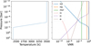 |
Fig. 2 Left panel: temperature-pressure (TP) profile used for our CC analysis, from Yan et al. (2023). Right panel: VMRs adapted in the single-species models used in this paper. The string ‘mol’ denotes each of the investigated molecules. |
3.4 GCM calculation
In this section, we model the phase-dependent thermal emission spectra of WASP-76 b to investigate how our detection maps (in terms of Kp and Vrest) are influenced by orbital Doppler shifts and line strength variations. Previous pRT-based models, which assume static 1D atmospheres, have proven effective for first-order studies aimed at detecting atmospheric species. However, they neglect longitudinal temperature gradients and phase-dependent variations in spectral line profiles. By adopting more realistic, 3D-informed models, we aimed to better interpret the observed emission and assess how atmospheric dynamics shape the detectability of species such as CO and Fe I. We followed the methodology described in Wardenier et al. (2025) to generate phase-dependent emission templates for Fe I and CO, based on a drag-free SPARC/MITgcm simulation of WASP-76 b (see also Wardenier et al. 2021, 2023). For details of the 3D temperature structure, chemistry, and dynamics, we refer the reader to Wardenier et al. (2025); here, we summarise the key aspects. The SPARC/MITgcm (Showman et al. 2009) is a nongrey global circulation model that has been used extensively to simulate the 3D climates of (ultra-)hot Jupiters. The dayside TP profile, shown in Figures 2 and 3 of Wardenier et al. (2025), exhibits a strong thermal inversion driven by the absorption of stellar irradiation by metals, with temperatures reaching up to ∼3500 K. This is consistent with the TP profile that we used to compute the 1D pRT model (Fig. 2). Chemical abundances in the GCM are calculated assuming local chemical equilibrium and solar metallicity. To obtain thermal emission spectra, we post-processed the model with the 3D radiative transfer code
gCMCRT (Lee et al. 2022). Templates were calculated at 10-degree phase intervals at a resolving power R = 300 000 and then convolved with the spectrograph instrument profile (following the same approach used for the 1D models)7. Furthermore, we included only the opacities of the relevant line species, either Fe I or CO, and the continuum (we used the same line lists as used for pRT; see Sect. 3.3). For each species, we computed two sets of templates: one accounting for Doppler shifts due to planetary rotation and wind profiles (‘3D templates with dynamics’), and one in which these shifts are disabled (‘3D templates without dynamics’; see the first row of Fig. 4 in Wardenier et al. 2025). The latter set still accounts for changes in the 3D temperature structure during the observation, but not for changes in Doppler shifts introduced by the planet’s atmosphere itself. The modelled wind field includes a day-to-night flow and a super-rotating equatorial jet, with wind speeds reaching up to ∼10 km/s.
4 Results
In this section, we summarise the results of our analysis. The main findings are presented in Table 3 and illustrated in Fig. 3.
4.1 Near-infrared: GIANO-B
We report a detection of CO in the GIANO-B data (see the first panel of Fig. 3) with an S/N of 10.4. The planetary signal is clearly visible on both nights, with S/N map peaks of 5.0 and 7.2 for Night 1 and Night 2, respectively (see Fig. A.1). This result confirms the detection previously reported by Yan et al. (2023) using the CRyogenic InfraRed Echelle Spectrograph (CRIRES) Upgrade, i.e. CRIRES+, which was based on single-night observations.
We also searched for Fe I in our GIANO-B data; however, we were unable to detect a clear peak in the CC map (see right panels of Fig. A.1 in the appendix). There appears to be only a hint of signal during the second night of observation at the expected position for a signal of planetary origin. The peak of the S/N map is located at Vrest = 14.5 ± 0.5 km s−1 and Kp =205.9 ± 0.7 km s−1, obtained by fitting a 2D Gaussian that includes a rotation angle to account for the tilted shape of the signal trace, reaching a maximum S/N of 4.0. Since we are probing less than a quarter of the planet’s orbit, we have the characteristic ‘degeneracy’ between Kp and Vrest, although the theoretical values still lies along the trail of the peak. Despite an S/N of 4.0, we refer to this detection as ‘marginal’ because it is present in only one of the two GIANO-B nights. Here, ‘marginal’ does not imply that the signal is statistically weak, but rather emphasises two factors: that the detection occurs in only one epoch and that the peak in the S/N map is slightly offset from the expected theoretical position.
4.2 Optical: HARPS-N and ESPRESSO
In the visible band, we detected Fe I in both HARPS-N (see the central panel of Fig. 3) and ESPRESSO (see the right panel of Fig. 3) spectra with S/N values of 3.5 and 6.2, respectively.
Costa Silva et al. (2024) first analysed ESPRESSO data of WASP-76 b’s dayside, reporting a consistent blueshift of −4.7 ± 0.3 km s−1 in the Fe I line. However, our re-analysis does not confirm this result, as our measured Vrest is consistent with 0 km s−1 (see Table 3). Our findings appear to be more in line with the GCM predictions by Wardenier et al. (2025), which suggest a negligible ∆Vrest when combining pre- and post-eclipse phases. Both the right panel of Fig. 3 and Table 4 show that the measured Kp exhibits a negative offset relative to the theoretical value of 196.52±0.94 km s−1.
In the analysis of the ESPRESSO data, we adopted a different strategy compared to Costa Silva et al. (2024), particularly in the pre-CC processing. Rather than applying the Molecfit tool (Smette et al. 2015; Kausch et al. 2015) for telluric correction, as performed by Costa Silva et al. (2024), we employed PCA, a technique widely adopted in the literature for CC-based studies. Moreover, while Costa Silva et al. (2024) used the RAS-SINE code (Cretignier et al. 2020) to remove the continuum and instrumental interference patterns (commonly referred to as ‘wiggles’), we applied a high-pass filter to eliminate low-frequency systematics that are not stable over time. We adopted a window of approximately 70 km s−1, chosen to be wide enough not to affect the planetary signal, yet narrow enough to correct for the wiggle frequencies (Bourrier et al. 2024). We verified through Lomb-Scargle periodograms that no significant periodicities remained in the post-PCA residuals. Our pre-CC methodology follows the standard framework originally developed for nIR data, which we have adapted and implemented here for optical spectroscopy. Furthermore, Costa Silva et al. (2024) employed an unweighted CC approach, whereas we followed the formalism of Gibson et al. (2020), Cont et al. (2022), and Nortmann et al. (2025) to account for uncertainties in the post-PCA residual spectra. To validate the performance of our analysis pipeline, we compared the CC maps, S/N maps, and final detections – using both injection tests and real data – with the results obtained from an independent tool previously adopted by our team for HARPS-N data analysis (see, e.g. Borsa et al. 2022). The two methods yielded fully consistent results.
Cross-correlation results.
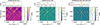 |
Fig. 3 Detection S/N maps as a function of Vrest and Kp for CO in GIANO-B (left panel), Fe I in HARPS-N (central panel), and Fe I in ESPRESSO (right panel) data. Dotted red and white lines mark the expected and obtained planetary positions, respectively. For each map, the top and right sub-panels show the 1D CC functions (in terms of S/N) at the peak position, with the best-fit Gaussian overplotted in orange. |
4.3 GCMs results
Wardenier et al. (2025) demonstrated how 3D atmospheric modelling can account for small offsets in the inferred orbital velocity, Kp, observed in emission spectroscopy, attributing these discrepancies to the 3D structure of WASP-76b’s atmosphere. Motivated by their findings, we also tested the application of GCMs in our analysis. We applied the GCMs on our most robust detections, namely CO in the GIANO-B spectra and Fe I in the ESPRESSO data. As highlighted in Sect. 3, we investigated two classes of atmospheric models: one excluding dynamical effects but including only a phase-dependent planetary atmosphere, i.e. a rotating 3D temperature structure without Doppler shifts, and one incorporating both wind and rotational broadening (see Fig. A.3). Within the dynamic framework, we compared a weak-drag model (with a drag timescale of 105 seconds; not shown here for conciseness) and a drag-free model, which showed the best agreement with the data. We adopted a likelihood-based comparison approach to evaluate which model is most consistent with the data. Specifically, we transformed the CC values into likelihood (LH) values following the formalism introduced by Gibson et al. (2020) and later adopted by Giacobbe et al. (2021). In this approach, the likelihood incorporates both the model line depths and the S/N across spectral orders and exposures. Detecting a peak in the LH map at the expected (Vrest, Kp) coordinates serves as a robust confirmation of the planetary signal. For each model, we computed a log-likelihood map over the (Vrest, Kp) parameter space by summing the contributions from each spectral order, observation, and RV shift, scanning Vrest values from −5 to +5 km s−1 in steps of 0.3 km s−1, and Kp from 186 km s−1 to 202 km s−1 in steps of 0.3 km s−1. To ensure consistency with our data reduction, we applied the same telluric correction and PCA-based filtering to the model spectra as to the observations. Finally, confidence levels on the detection were derived using the likelihood-ratio test, comparing each point on the (Vrest, Kp) grid to the maximum LH value.
The results are shown in Fig. 4. Although there is no significant advantage in terms of LH between the dynamic and non-dynamic 3D models (the non-drag dynamic model is only favoured by δ log(L) = 2 compared to the drag-free model without Doppler effects), applying 3D GCMs yields a clear improvement in Kp -Vrest space. For non-dynamic models, the LH peak is incompatible with the theoretical planetary position. Even when considering the uncertainty of approximately 1 km s−1 on the theoretical Kp (see Table 1), the 3σ interval does not overlap with the 3σ confidence range of the model without dynamics.
Conversely, when adopting GCMs with atmospheric dynamics, i.e. the drag-free model, the LH peak becomes consistent with the expected Vrest and Kp values within 1 to 2σ (when accounting for the error of 1 km s−1 on the theoretical Kp). The physical aspect of the GCM responsible for the better fit is the fact that we account for phase-dependent Doppler shifts due to planetary rotation and the wind profile (see Fig. 11 in Wardenier et al. 2025). For completeness, we also tested the weak-drag dynamical model, which resulted in a detection compatible with the theoretical Kp and Vrest values at the 3σ level. However, because the agreement between this model and our data is worse than that of the drag-free model, we do not discuss it further here. Our result agrees with Ehrenreich et al. (2020), who pointed out that a hotspot offset is in tension with the possible existence of strong drag forces.
Regarding the application of GCMs to our GIANO-B data, our results are inconclusive, as both the drag-free and nondynamic models are consistent within 1σ with the theoretically expected position for a planetary signal, possibly due to the limitations imposed by the lower S/N (Pluriel 2023). However, it is worth noting that, according to Table 3, the observed Kp for CO is consistent with the expected Kp from the literature within the uncertainties. Consequently, there is no conclusive evidence for a non-zero ∆Kp, and thus for significant 3D effects. To better assess the role of dynamics, more precise measurements of Kp from the CO CC analysis would be required.
GCM results.
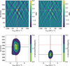 |
Fig. 4 Comparison between 3D templates with dynamics (left panels) and 3D templates without dynamics (right panels) for Fe I in ESPRESSO data. Top panels: Detection S/N maps as a function of Kp and Vrest with the 1D CC functions (see Fig 3 for details). Bottom panels: Likelihood confidence intervals as a function of Kp and Vrest. Dotted red and black lines mark the expected and obtained planetary positions, respectively. The 3D templates are computed based on the drag-free GCM of WASP-76 b from Wardenier et al. (2025). |
5 Discussion and conclusion
In this paper, we analysed two observations of the dayside of WASP-76 b obtained with the GIARPS observing mode of the TNG, which combines the two high-resolution spectrographs GIANO-B in the nIR and HARPS-N in the optical. Additionally, we reanalysed four nights of publicly available ESPRESSO data, which were initially examined by Costa Silva et al. (2024).
Our primary goal was to study multi-band spectra to achieve the best possible characterisation of CO and Fe I, two key tracers of the dynamics and thermal structure of the planetary dayside. A crucial aspect of our work was the application of a consistent analysis approach to both nIR and optical datasets.
We detected CO in our GIANO-B spectra with an S/N of 10.4, confirming the previous detection obtained with CRIRES+ by Yan et al. (2023). Additionally, we report the detection of Fe I with S/N values of 3.5 and 6.2 for HARPS-N and ESPRESSO, respectively. However, for ESPRESSO data, we were unable to reproduce the blueshifted signal reported by Costa Silva et al. (2024). The retrieved values of Kp and Vrest are consistent with theoretical predictions or show a small deviation in ∆Kp (∆Kp ∼6 km s−1 compatible with the theoretical Kp of ∼196 km s−1 (see Table 1) at the ∼4σ level. This deviation was calculated by averaging the Kp values and their respective uncertainties listed in Table 3, consistent with the findings of Wardenier et al. (2025).
A ‘marginal’ detection of Fe I is also suggested in the GIANO-B data (see the right panel of Fig. A.1 in the appendix), although the signal is embedded in a noisy map. However, we verified through injection-recovery tests that the spurious peaks are unlikely to be caused by cross-contamination from other molecular or atomic species (i.e. Cr, H2O, OH, CO, CO2, or Mg). This is an important check, especially in the case of a few Fe I lines. While this may not yet qualify as a robust detection, we observe that the LH significance of the Fe I detection improves when combining the most favourable GIANO-B night with the HARPS-N data (see Fig. A.4). Although the detection is still primarily driven by HARPS-N, GIANO-B contributes by enhancing the signal and reducing the presence of spurious peaks in the LH map. We stress that, even though we consider the Fe I detection with GIANO-B as ‘marginal’ for the reasons explained in Sect. 4.1, its genuineness is somewhat strengthened by the corresponding detection with HARPS-N. Specifically, GIANO-B confirms the same features detected with HARPS-N.
Furthermore, in this work, we tested GCM-based models for CC, particularly to verify the theoretical predictions that GCMs can resolve the small discrepancies in retrieved Kp values typically observed when using simplified 1D models. This study represents one of the few applications of GCMs in both CC and LH frameworks applied to real data (see, e.g. Flowers et al. 2019, Beltz et al. 2021). Although, from a statistical perspective, the LH framework favours the dynamic GCM by only δ log(L) = 2 in our ESPRESSO analysis (see Table 4), the LH maps in Fig. 4 clearly show that – at the 2σ level – only the dynamic model aligns with the expected planetary velocity. In contrast, a static model fails to reproduce this offset. We find that only the drag-free GCM reproduces the magnitude of the Kp offset seen in the ESPRESSO data. A weak-drag model (with lower wind speeds and no super-rotating equatorial jet) cannot fully reproduce the size of the Kp offset seen in the data.
We note that in both HARPS-N and GIANO-B data, the planetary iron signal appears to be stronger during the posteclipse, with S/N and likelihood maps showing fewer spurious features during the post-eclipse night (see the right panels of Fig. A.1 for GIANO-B and Fig. A.5 for HARPS-N in the appendix). Although the CO signal is detected on both nights, some effects –possibly instrumental issues or weather conditions– may have affected our measurements during the first GIARPS observation. However, since CO remains detectable during Night 1 and the night logs report no significant differences in weather conditions, the origin of this nightly variation remains unclear. Given the intrinsically weaker detection of the Fe I signal compared to CO, it remains plausible that some instrumental issues may have impacted our GIANO-B results during Night 1. It should be noted that Yan et al. (2020) observed a similar effect in the atmosphere of WASP-189 b, with a stronger Fe I signal just after the secondary eclipse event. However, they attributed this difference to a lower S/N in the pre-eclipse observation, likely caused by a telescope focussing issue. According to Fig. 2, the strongest detections in our GIARPS observations also correspond to a higher S/N ratio. Interestingly, our re-analysis of the ESPRESSO data reveals that Fe I also appears weaker in pre-eclipse than in post-eclipse observations (see Fig. A.6 and Table A.2).
The stronger Fe I detection at post-eclipse phases is consistent with the idea that the hotspot is shifted from the substellar point towards the evening terminator, as often seen in phase curve observations (e.g. Wong et al. 2016). As shown in van Sluijs et al. (2023) and Wardenier et al. (2025), the vertical temperature gradient is stronger outside the hotspot than inside. Because the strength of the emission lines is set by the temperature gradient (and not by the absolute temperature), we expect the emission signal to be stronger than in pre-eclipse, during which most of the hotspot is in view. A similar explanation was also given for Kelt-20 b by Borsa et al. (2022), who found an asymmetric detection of Fe II and Cr I detected only after the occultation and not before, hinting at different atmospheric properties during the pre- and post-occultation orbital phases.
This asymmetry in WASP-76 b’s atmosphere may indicate the presence of zonal flows that transport heat longitudinally in a prograde direction (aligned with the tidally locked solid-body rotation,  deg; Ehrenreich et al. 2020) in the upper atmosphere, which would shift the hotspot position eastward. This effect may be observed only with Fe I (and not with CO) because Fe I forms higher in the atmosphere at higher temperatures. This is largely consistent with the findings of Ehrenreich et al. (2020), who introduced a hotspot offset toward the evening terminator to explain the asymmetry observed between the ingress and egress phases of WASP-76 b’s transit. It is also consistent with theoretical studies (e.g. Showman & Polvani 2011 and Parmentier & Crossfield 2018), which suggest that eastward shifts in thermal phase curves are a robust outcome of hot Jupiter circulation regimes. However, May et al. (2021) analysed the IR phase curves of WASP-76 b and found little to no asymmetry, a result confirmed by a reanalysis of Demangeon et al. (2024) and Dang et al. (2025). Notably, Demangeon et al. (2024) also examined phase curves in the optical regime using Transiting Exoplanet Survey Satellite (TESS) and CHaracterising ExOPlanets Satellite (CHEOPS) data, identifying a peak flux excess before the eclipse that suggests a tentative asymmetry in the phase curve at visible wavelengths. This asymmetry could indicate an asymmetric wind pattern from west to east in the atmospheric layers probed at visible wavelengths. As noted by May et al. (2021), the dynamics of atmospheric layers probed at visible and IR wavelengths may differ. An alternative explanation for the hint of asymmetry in the optical light curves invoked by Demangeon et al. (2024) is scattering, the ‘glory effect’, and associated clouds in the eastern hemisphere. However, this hypothesis is challenged by theoretical predictions that clouds should form in the western hemisphere (e.g. Hu et al. 2015; Parmentier et al. 2016; Lee et al. 2016; Helling et al. 2019). In Fig. A.7, we graphically illustrate the two different explanations for the asymmetry in the Fe I detection between the pre- and post-eclipse phases highlighted in this section. From a preliminary analysis of JWST/NIRSpec data (private communication, JWST GO 5268, PI: Wardenier), non-zero eastward offsets of ∼5 degrees appear to be present, reinforcing our hypothesis that a difference in the temperature gradient may cause the Fe I asymmetry hinted at between the pre- and post-eclipse phases.
This work represents one of the first steps toward conducting similar studies on a larger sample of exoplanets within the framework of the GAPS programme. The GAPS programme at the TNG has collected multiple transits (ranging from three to eleven) for a key sample of approximately 40 exoplanets using GIARPS, building a unique and unparalleled dataset for the astronomical community in the coming years. This dataset will enable detailed studies on the repeatability of atmospheric detections and the variability of exoplanetary atmospheres, laying the groundwork for future investigations with the Extremely Large Telescope (ELT). Furthermore, we plan to combine our observations with publicly available archival ESPRESSO and CRIRES+ data to take advantage of the highest-resolution spectrographs currently available. In cases of high S/N detections, we will also be able to test GCMs when available, as demonstrated in this work. Observational constraints are essential for GCMs. For instance, to measure the impact of drag would require more observations of hot Jupiters and ultra-hot Jupiters to be fully modelled. The detection of species with accurate abundances would also help to determine the atmospheric regime (e.g. equilibrium, non-equilibrium, etc.), which has a significant impact on GCMs, as shown by Pluriel (2023).
Acknowledgements
We thank the anonymous referee for their valuable feedback on this paper. We are also grateful to A. Chiavassa for his kind and insightful support in our efforts to model the stellar contamination. We acknowledge the Italian Centre for Astronomical Archives (IA2, https://www.ia2.inaf.it), part of the Italian National Institute for Astrophysics (INAF), for providing technical assistance, services and supporting activities of the GAPS collaboration. We acknowledge A. Lanza for very helpful comments on the manuscript. J.P.W. acknowledges support from the Trottier Family Foundation via the Trottier Postdoctoral Fellowship held at IREx and the Canadian Space Agency (CSA) under grant 24JWGO3A-03. The authors acknowledge financial contributions from PRIN INAF 2019 and INAF GO Large Grant 2023 GAPS-2 as well as from the European Union – Next Generation EU RRF M4C2 1.1 PRIN MUR 2022 project 2022CERJ49 (ESPLORA). P.E.C. is funded by the Austrian Science Fund (FWF) Erwin Schroedinger Fellowship, program J4595-N. Part of the research activities described in this paper were carried out with contribution of the Next Generation EU funds within the National Recovery and Resilience Plan (PNRR), Mission 4 – Education and Research, Component 2 – From Research to Business (M4C2), Investment Line 3.1 – Strengthening and creation of Research Infrastructures, Project IR0000034 – “STILES – Strengthening the Italian Leadership in ELT and SKA”.
Appendix A Additional figures and tables
Number of PCA components used in this analysis
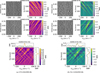 |
Fig. A.1 Cross-correlation results for CO (left panels) and Fe I (right panels) in GIANO-B data. For each species, we show the results for individual nights (top two rows) and their combined signal (bottom row). The greyscale maps represent the CC functions as a function of velocity in the telluric rest frame (Vtell) and orbital phase. Masked regions are affected by stellar residuals (see Sect. 3). The black and white dashed lines indicate the stellar and planetary trails, respectively. |
The colour maps display the 2D CC function in the (Kp, Vrest) plane, expressed in terms of S/N. A detailed description of these plots is provided in the caption of Fig. 3. Since we adopted the CC approach from Gibson et al. (2020), Cont et al. (2022), and Nortmann et al. (2025), the noisier lines have larger uncertainties, and a bigger relative scatter among the data.
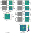 |
Fig. A.2 Cross-correlation results for Fe I in HARPS-N (left panels) and ESPRESSO (right panels) data. Same as Fig. A.1. The ESPRESSO CC grey maps are in the barycentric rest frame. |
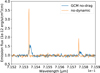 |
Fig. A.3 Emission flux as a function of wavelength, computed at a phase angle of approximately 0.583, for both the drag-free GCM (in blue) and the ’static’ model (in orange), in a region around a Fe I line. |
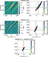 |
Fig. A.4 Fe I detection with GIARPS during Night 2. For each instrument (top row: GIANO-B; middle row: HARPS-N), we present: the 2D CC maps in the (Kp, Vrest) plane, expressed in terms of S/N (left panels, colour scale); and the corresponding likelihood confidence interval maps (right panels). The bottom row shows the combined GIANO-B + HARPS-N confidence interval maps. Although the detection is primarily driven by HARPS-N, GIANO-B contributes by cleaning the signal and reducing spurious peaks in the likelihood maps. |
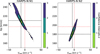 |
Fig. A.5 Likelihood confidence interval maps of Fe I detection with HARPS-N as a function of Vrest and Kp. Red (black) dotted lines mark the expected (obtained) planetary position. |
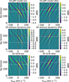 |
Fig. A.6 Detection of Fe I with ESPRESSO during pre-eclipse (left panels) and post-eclipse (right panels). For each atmospheric model (top row: 1D pRT; middle row: 3D without dynamics; bottom row: 3D nodrag GCM), we present the two-dimensional CC maps in the (Kp, Vrest) plane, expressed in terms of S/N (see Fig. A.1 for more details). |
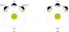 |
Fig. A.7 Possible explanation for the asymmetry of our detection. a) panel, the asymmetry could be due to the eastward shift of the hotspot. During the pre-eclipse phase (when we observe the eastern side with the hotspot), the observed temperature gradient is shallower. The temperature gradient is steeper during the post-eclipse phase (when we observe more of the western side). As a result, the spectral line contrast (linked to these gradients) will be weaker before the eclipse and stronger after the eclipse. b) panel, the fainter detection during pre-eclipse compared to post-eclipse observations could be due to the presence of clouds and the associated glory effect in the eastern hemisphere, a hint of this could be the hotspot offset detected in the optical CHEOPS and TESS light curves. |
References
- Arcangeli, J., Désert, J.-M., Line, M. R., et al. 2018, ApJ, 855, L30 [Google Scholar]
- Azevedo Silva, T., Demangeon, O. D. S., Santos, N. C., et al. 2022, A&A, 666, L10 [NASA ADS] [CrossRef] [EDP Sciences] [Google Scholar]
- Basilicata, M., Giacobbe, P., Bonomo, A. S., et al. 2024, A&A, 686, A127 [NASA ADS] [CrossRef] [EDP Sciences] [Google Scholar]
- Baxter, C., Désert, J.-M., Parmentier, V., et al. 2020, A&A, 639, A36 [EDP Sciences] [Google Scholar]
- Beltz, H., Rauscher, E., Brogi, M., & Kempton, E. M. R. 2021, AJ, 161, 1 [Google Scholar]
- Birkby, J. L. 2018, in Handbook of Exoplanets, eds. H. J. Deeg, & J. A. Belmonte, 16 [Google Scholar]
- Birkby, J. L., de Kok, R. J., Brogi, M., et al. 2013, MNRAS, 436, L35 [Google Scholar]
- Bohn, A. J., Southworth, J., Ginski, C., et al. 2020, A&A, 635, A73 [NASA ADS] [CrossRef] [EDP Sciences] [Google Scholar]
- Borsa, F., Giacobbe, P., Bonomo, A. S., et al. 2022, A&A, 663, A141 [NASA ADS] [CrossRef] [EDP Sciences] [Google Scholar]
- Borysow, A. 2002, A&A, 390, 779 [NASA ADS] [CrossRef] [EDP Sciences] [Google Scholar]
- Borysow, A., & Frommhold, L. 1989, ApJ, 341, 549 [NASA ADS] [CrossRef] [Google Scholar]
- Borysow, J., Frommhold, L., & Birnbaum, G. 1988, ApJ, 326, 509 [NASA ADS] [CrossRef] [Google Scholar]
- Borysow, A., Frommhold, L., & Moraldi, M. 1989, ApJ, 336, 495 [NASA ADS] [CrossRef] [Google Scholar]
- Borysow, A., Jorgensen, U. G., & Fu, Y. 2001, J. Quant. Spec. Radiat. Transf., 68, 235 [NASA ADS] [CrossRef] [Google Scholar]
- Bourrier, V., Delisle, J. B., Lovis, C., et al. 2024, A&A, 691, A113 [NASA ADS] [CrossRef] [EDP Sciences] [Google Scholar]
- Brogi, M., & Birkby, J. 2021, in ExoFrontiers; Big Questions in Exoplanetary Science, ed. N. Madhusudhan, 8 [Google Scholar]
- Brogi, M., Snellen, I. A. G., de Kok, R. J., et al. 2012, Nature, 486, 502 [Google Scholar]
- Brogi, M., de Kok, R. J., Birkby, J. L., Schwarz, H., & Snellen, I. A. G. 2014, A&A, 565, A124 [NASA ADS] [CrossRef] [EDP Sciences] [Google Scholar]
- Brogi, M., de Kok, R. J., Albrecht, S., et al. 2016, ApJ, 817, 106 [Google Scholar]
- Brogi, M., Giacobbe, P., Guilluy, G., et al. 2018, A&A, 615, A16 [NASA ADS] [CrossRef] [EDP Sciences] [Google Scholar]
- Carleo, I., Giacobbe, P., Guilluy, G., et al. 2022, AJ, 164, 101 [NASA ADS] [CrossRef] [Google Scholar]
- Chiavassa, A., & Brogi, M. 2019, A&A, 631, A100 [NASA ADS] [CrossRef] [EDP Sciences] [Google Scholar]
- Casasayas-Barris, N., Orell-Miquel, J., Stangret, M., et al. 2021, A&A, 654, A163 [NASA ADS] [CrossRef] [EDP Sciences] [Google Scholar]
- Claudi, R., Benatti, S., Carleo, I., et al. 2017, Eur. Phys. J. Plus, 132, 364 [NASA ADS] [CrossRef] [Google Scholar]
- Cont, D., Yan, F., Reiners, A., et al. 2022, A&A, 668, A53 [NASA ADS] [CrossRef] [EDP Sciences] [Google Scholar]
- Cosentino, R., Lovis, C., Pepe, F., et al. 2012, SPIE Conf. Ser., 8446, 84461V [Google Scholar]
- Costa Silva, A. R., Demangeon, O. D. S., Santos, N. C., et al. 2024, A&A, 689, A8 [NASA ADS] [CrossRef] [EDP Sciences] [Google Scholar]
- Covino, E., Esposito, M., Barbieri, M., et al. 2013, A&A, 554, A28 [NASA ADS] [CrossRef] [EDP Sciences] [Google Scholar]
- Cretignier, M., Francfort, J., Dumusque, X., Allart, R., & Pepe, F. 2020, A&A, 640, A42 [NASA ADS] [CrossRef] [EDP Sciences] [Google Scholar]
- Dang, L., Bell, T. J., Shu, Y. Z., et al. 2025, AJ, 169, 32 [NASA ADS] [CrossRef] [Google Scholar]
- Deibert, E. K., de Mooij, E. J. W., Jayawardhana, R., et al. 2021, ApJ, 919, L15 [NASA ADS] [CrossRef] [Google Scholar]
- Deibert, E. K., de Mooij, E. J. W., Jayawardhana, R., et al. 2023, AJ, 166, 141 [NASA ADS] [CrossRef] [Google Scholar]
- Demangeon, O. D. S., Cubillos, P. E., Singh, V., et al. 2024, A&A, 684, A27 [NASA ADS] [CrossRef] [EDP Sciences] [Google Scholar]
- Edwards, B., Changeat, Q., Baeyens, R., et al. 2020, AJ, 160, 8 [Google Scholar]
- Ehrenreich, D., Lovis, C., Allart, R., et al. 2020, Nature, 580, 597 [Google Scholar]
- Flowers, E., Brogi, M., Rauscher, E., Kempton, E. M. R., & Chiavassa, A. 2019, AJ, 157, 209 [Google Scholar]
- Fu, G., Deming, D., Lothringer, J., et al. 2021, AJ, 162, 108 [NASA ADS] [CrossRef] [Google Scholar]
- Gaia Collaboration (Spoto, F., et al.) 2018, A&A, 616, A13 [NASA ADS] [CrossRef] [EDP Sciences] [Google Scholar]
- Gandhi, S., Kesseli, A., Snellen, I., et al. 2022, MNRAS, 515, 749 [NASA ADS] [CrossRef] [Google Scholar]
- Gandhi, S., Madhusudhan, N., & Mandell, A. 2020, AJ, 159, 232 [Google Scholar]
- Gandhi, S., Kesseli, A., Zhang, Y., et al. 2023, AJ, 165, 242 [NASA ADS] [CrossRef] [Google Scholar]
- Garhart, E., Deming, D., Mandell, A., et al. 2020, AJ, 159, 137 [NASA ADS] [CrossRef] [Google Scholar]
- Giacobbe, P., Brogi, M., Gandhi, S., et al. 2021, Nature, 592, 205 [NASA ADS] [CrossRef] [Google Scholar]
- Gibson, N. P., Merritt, S., Nugroho, S. K., et al. 2020, MNRAS, 493, 2215 [Google Scholar]
- Ginski, C., Mugrauer, M., Seeliger, M., et al. 2016, MNRAS, 457, 2173 [Google Scholar]
- Gray, D. F. 1992, The Observation and Analysis of Stellar Photospheres, 20 [Google Scholar]
- Guilluy, G., Giacobbe, P., Carleo, I., et al. 2022, A&A, 665, A104 [NASA ADS] [CrossRef] [EDP Sciences] [Google Scholar]
- Helling, C., Iro, N., Corrales, L., et al. 2019, A&A, 631, A79 [NASA ADS] [CrossRef] [EDP Sciences] [Google Scholar]
- Hoeijmakers, H. J., Ehrenreich, D., Kitzmann, D., et al. 2019, A&A, 627, A165 [NASA ADS] [CrossRef] [EDP Sciences] [Google Scholar]
- Hu, R., Demory, B.-O., Seager, S., Lewis, N., & Showman, A. P. 2015, ApJ, 802, 51 [Google Scholar]
- Kausch, W., Noll, S., Smette, A., et al. 2015, A&A, 576, A78 [NASA ADS] [CrossRef] [EDP Sciences] [Google Scholar]
- Kawauchi, K., Narita, N., Sato, B., & Kawashima, Y. 2022, PASJ, 74, 225 [CrossRef] [Google Scholar]
- Kesseli, A. Y., & Snellen, I. A. G. 2021, ApJ, 908, L17 [Google Scholar]
- Kesseli, A. Y., Snellen, I. A. G., Casasayas-Barris, N., Mollière, P., & Sánchez-López, A. 2022, AJ, 163, 107 [NASA ADS] [CrossRef] [Google Scholar]
- Landman, R., Sánchez-López, A., Mollière, P., et al. 2021, A&A, 656, A119 [NASA ADS] [CrossRef] [EDP Sciences] [Google Scholar]
- Lee, E., Dobbs-Dixon, I., Helling, C., Bognar, K., & Woitke, P. 2016, A&A, 594, A48 [NASA ADS] [CrossRef] [EDP Sciences] [Google Scholar]
- Lee, E. K. H., Wardenier, J. P., Prinoth, B., et al. 2022, ApJ, 929, 180 [NASA ADS] [CrossRef] [Google Scholar]
- Louden, T., & Wheatley, P. J. 2015, ApJ, 814, L24 [CrossRef] [Google Scholar]
- Maguire, C., Gibson, N. P., Nugroho, S. K., et al. 2024, A&A, 687, A49 [NASA ADS] [CrossRef] [EDP Sciences] [Google Scholar]
- Malik, M., Grosheintz, L., Mendonça, J. M., et al. 2017, AJ, 153, 56 [Google Scholar]
- Masson, A., Vinatier, S., Bézard, B., et al. 2024, A&A, 688, A179 [NASA ADS] [CrossRef] [EDP Sciences] [Google Scholar]
- May, E. M., Komacek, T. D., Stevenson, K. B., et al. 2021, AJ, 162, 158 [NASA ADS] [CrossRef] [Google Scholar]
- Mollière, P., Wardenier, J. P., van Boekel, R., et al. 2019, A&A, 627, A67 [Google Scholar]
- Ngo, H., Knutson, H. A., Hinkley, S., et al. 2016, ApJ, 827, 8 [Google Scholar]
- Nortmann, L., Lesjak, F., Yan, F., et al. 2025, A&A, 693, A213 [NASA ADS] [CrossRef] [EDP Sciences] [Google Scholar]
- Parmentier, V., & Crossfield, I. J. M. 2018, in Handbook of Exoplanets, eds. H. J. Deeg, & J. A. Belmonte, 116 [Google Scholar]
- Parmentier, V., Fortney, J. J., Showman, A. P., Morley, C., & Marley, M. S. 2016, ApJ, 828, 22 [Google Scholar]
- Parmentier, V., Line, M. R., Bean, J. L., et al. 2018, A&A, 617, A110 [NASA ADS] [CrossRef] [EDP Sciences] [Google Scholar]
- Pelletier, S., Benneke, B., Ali-Dib, M., et al. 2023, Nature, 619, 491 [NASA ADS] [CrossRef] [Google Scholar]
- Pepe, F., Cristiani, S., Rebolo, R., et al. 2021, A&A, 645, A96 [NASA ADS] [CrossRef] [EDP Sciences] [Google Scholar]
- Pino, L., Désert, J.-M., Brogi, M., et al. 2020, ApJ, 894, L27 [Google Scholar]
- Pino, L., Brogi, M., Désert, J. M., et al. 2022, A&A, 668, A176 [NASA ADS] [CrossRef] [EDP Sciences] [Google Scholar]
- Pluriel, W. 2023, Remote Sensing, 15, 635 [NASA ADS] [CrossRef] [Google Scholar]
- Press, W. H., Teukolsky, S. A., Vetterling, W. T., & Flannery, B. P. 2007, Numerical Recipes: The Art of Scientific Computing (Cambridge: Cambridge University Press) [Google Scholar]
- Rainer, M., Harutyunyan, A., Carleo, I., et al. 2018, SPIE Conf. Ser., 10702, 1070266 [Google Scholar]
- Rauscher, E., & Kempton, E. M. R. 2014, ApJ, 790, 79 [NASA ADS] [CrossRef] [Google Scholar]
- Rothman, L. S., Gordon, I. E., Barber, R. J., et al. 2010, J. Quant. Spec. Radiat. Transf., 111, 2139 [NASA ADS] [CrossRef] [Google Scholar]
- Sánchez-López, A., Landman, R., Mollière, P., et al. 2022, A&A, 661, A78 [NASA ADS] [CrossRef] [EDP Sciences] [Google Scholar]
- Savel, A. B., Kempton, E. M. R., Malik, M., et al. 2022, ApJ, 926, 85 [NASA ADS] [CrossRef] [Google Scholar]
- Seidel, J. V., Ehrenreich, D., Wyttenbach, A., et al. 2019, A&A, 623, A166 [NASA ADS] [CrossRef] [EDP Sciences] [Google Scholar]
- Seidel, J. V., Ehrenreich, D., Pino, L., et al. 2020, A&A, 633, A86 [NASA ADS] [CrossRef] [EDP Sciences] [Google Scholar]
- Seidel, J. V., Prinoth, B., Pino, L., et al. 2025, Nature, 639, 902 [Google Scholar]
- Seidel, J. V., Ehrenreich, D., Allart, R., et al. 2021, A&A, 653, A73 [NASA ADS] [CrossRef] [EDP Sciences] [Google Scholar]
- Showman, A. P., & Polvani, L. M. 2011, ApJ, 738, 71 [Google Scholar]
- Showman, A. P., Fortney, J. J., Lian, Y., et al. 2009, ApJ, 699, 564 [NASA ADS] [CrossRef] [Google Scholar]
- Showman, A. P., Cho, J. Y. K., & Menou, K. 2010, in Exoplanets, ed. S. Seager, 471 [Google Scholar]
- Showman, A. P., Fortney, J. J., Lewis, N. K., & Shabram, M. 2013, ApJ, 762, 24 [Google Scholar]
- Smette, A., Sana, H., Noll, S., et al. 2015, A&A, 576, A77 [NASA ADS] [CrossRef] [EDP Sciences] [Google Scholar]
- Snellen, I. A. G., de Kok, R. J., de Mooij, E. J. W., & Albrecht, S. 2010, Nature, 465, 1049 [Google Scholar]
- Stangret, M., Fossati, L., D’Arpa, M. C., et al. 2024, A&A, 692, A76 [NASA ADS] [CrossRef] [EDP Sciences] [Google Scholar]
- Tabernero, H. M., Zapatero Osorio, M. R., Allart, R., et al. 2021, A&A, 646, A158 [NASA ADS] [CrossRef] [EDP Sciences] [Google Scholar]
- van Sluijs, L., Birkby, J. L., Lothringer, J., et al. 2023, MNRAS, 522, 2145 [NASA ADS] [CrossRef] [Google Scholar]
- Wardenier, J. P., Parmentier, V., Lee, E. K. H., Line, M. R., & Gharib-Nezhad, E. 2021, MNRAS, 506, 1258 [NASA ADS] [CrossRef] [Google Scholar]
- Wardenier, J. P., Parmentier, V., Line, M. R., & Lee, E. K. H. 2023, MNRAS, 525, 4942 [NASA ADS] [CrossRef] [Google Scholar]
- Wardenier, J. P., Parmentier, V., Lee, E. K. H., & Line, M. R. 2025, ApJ, 986, 63 [Google Scholar]
- Weiner Mansfield, M., Line, M. R., Wardenier, J. P., et al. 2024, AJ, 168, 14 [NASA ADS] [CrossRef] [Google Scholar]
- West, R. G., Hellier, C., Almenara, J. M., et al. 2016, A&A, 585, A126 [NASA ADS] [CrossRef] [EDP Sciences] [Google Scholar]
- Wöllert, M., & Brandner, W. 2015, A&A, 579, A129 [NASA ADS] [CrossRef] [EDP Sciences] [Google Scholar]
- Wong, I., Knutson, H. A., Kataria, T., et al. 2016, ApJ, 823, 122 [NASA ADS] [CrossRef] [Google Scholar]
- Wyttenbach, A., Ehrenreich, D., Lovis, C., Udry, S., & Pepe, F. 2015, A&A, 577, A62 [NASA ADS] [CrossRef] [EDP Sciences] [Google Scholar]
- Yan, F., Pallé, E., Reiners, A., et al. 2020, A&A, 640, L5 [NASA ADS] [CrossRef] [EDP Sciences] [Google Scholar]
- Yan, F., Reiners, A., Pallé, E., et al. 2022, A&A, 659, A7 [NASA ADS] [CrossRef] [EDP Sciences] [Google Scholar]
- Yan, F., Nortmann, L., Reiners, A., et al. 2023, A&A, 672, A107 [NASA ADS] [CrossRef] [EDP Sciences] [Google Scholar]
We adopted constant-with-altitude VMRs, as ionised CO and Fe I are disfavoured in the atmosphere of WASP-76 b. This is because (i) higher temperatures are predicted to dissociate CO’s strong triple bond, and (ii) Costa Silva et al. (2024) reports a non-detection of Fe II in this planet’s atmosphere.
We emphasise that, in our case, SVD is not used to decompose the signal – as is common in the field – but rather as a numerically robust method to solve a linear system. SVD is particularly well suited for solving systems involving matrices that are singular or nearly singular, as it offers improved numerical stability compared to other numerical equations (Press et al. 2007).
We verified through injection-recovery tests that this filtering process does not alter the planetary signal. Additionally, since the planetary signal varies significantly with time in the telluric-barycentric rest frame, the filter, being applied column-wise, affects only one temporal element per RV, and thus its impact on the planetary signal is expected to be negligible.
Since the grid of models is uniformly calculated at 10-degree phase intervals, for each observation in our dataset, we selected the grid model with the closest phase to that of the observation.
All Tables
All Figures
|
Fig. 1 Top panel: schematic representation of the orbit of WASP-76 b. The orbital phases covered in this study with GIARPS are colour-coded according to observing night. Bottom panel: S/N averaged over orders as a function of the orbital phase for nights in emission. The markers’ colour is proportional to the airmass. The exposures with higher S/N are from HARPS-N, while those with lower S/N are from GIANO-B. |
| In the text | |
|
Fig. 2 Left panel: temperature-pressure (TP) profile used for our CC analysis, from Yan et al. (2023). Right panel: VMRs adapted in the single-species models used in this paper. The string ‘mol’ denotes each of the investigated molecules. |
| In the text | |
|
Fig. 3 Detection S/N maps as a function of Vrest and Kp for CO in GIANO-B (left panel), Fe I in HARPS-N (central panel), and Fe I in ESPRESSO (right panel) data. Dotted red and white lines mark the expected and obtained planetary positions, respectively. For each map, the top and right sub-panels show the 1D CC functions (in terms of S/N) at the peak position, with the best-fit Gaussian overplotted in orange. |
| In the text | |
|
Fig. 4 Comparison between 3D templates with dynamics (left panels) and 3D templates without dynamics (right panels) for Fe I in ESPRESSO data. Top panels: Detection S/N maps as a function of Kp and Vrest with the 1D CC functions (see Fig 3 for details). Bottom panels: Likelihood confidence intervals as a function of Kp and Vrest. Dotted red and black lines mark the expected and obtained planetary positions, respectively. The 3D templates are computed based on the drag-free GCM of WASP-76 b from Wardenier et al. (2025). |
| In the text | |
|
Fig. A.1 Cross-correlation results for CO (left panels) and Fe I (right panels) in GIANO-B data. For each species, we show the results for individual nights (top two rows) and their combined signal (bottom row). The greyscale maps represent the CC functions as a function of velocity in the telluric rest frame (Vtell) and orbital phase. Masked regions are affected by stellar residuals (see Sect. 3). The black and white dashed lines indicate the stellar and planetary trails, respectively. |
| In the text | |
|
Fig. A.2 Cross-correlation results for Fe I in HARPS-N (left panels) and ESPRESSO (right panels) data. Same as Fig. A.1. The ESPRESSO CC grey maps are in the barycentric rest frame. |
| In the text | |
|
Fig. A.3 Emission flux as a function of wavelength, computed at a phase angle of approximately 0.583, for both the drag-free GCM (in blue) and the ’static’ model (in orange), in a region around a Fe I line. |
| In the text | |
|
Fig. A.4 Fe I detection with GIARPS during Night 2. For each instrument (top row: GIANO-B; middle row: HARPS-N), we present: the 2D CC maps in the (Kp, Vrest) plane, expressed in terms of S/N (left panels, colour scale); and the corresponding likelihood confidence interval maps (right panels). The bottom row shows the combined GIANO-B + HARPS-N confidence interval maps. Although the detection is primarily driven by HARPS-N, GIANO-B contributes by cleaning the signal and reducing spurious peaks in the likelihood maps. |
| In the text | |
|
Fig. A.5 Likelihood confidence interval maps of Fe I detection with HARPS-N as a function of Vrest and Kp. Red (black) dotted lines mark the expected (obtained) planetary position. |
| In the text | |
|
Fig. A.6 Detection of Fe I with ESPRESSO during pre-eclipse (left panels) and post-eclipse (right panels). For each atmospheric model (top row: 1D pRT; middle row: 3D without dynamics; bottom row: 3D nodrag GCM), we present the two-dimensional CC maps in the (Kp, Vrest) plane, expressed in terms of S/N (see Fig. A.1 for more details). |
| In the text | |
|
Fig. A.7 Possible explanation for the asymmetry of our detection. a) panel, the asymmetry could be due to the eastward shift of the hotspot. During the pre-eclipse phase (when we observe the eastern side with the hotspot), the observed temperature gradient is shallower. The temperature gradient is steeper during the post-eclipse phase (when we observe more of the western side). As a result, the spectral line contrast (linked to these gradients) will be weaker before the eclipse and stronger after the eclipse. b) panel, the fainter detection during pre-eclipse compared to post-eclipse observations could be due to the presence of clouds and the associated glory effect in the eastern hemisphere, a hint of this could be the hotspot offset detected in the optical CHEOPS and TESS light curves. |
| In the text | |
Current usage metrics show cumulative count of Article Views (full-text article views including HTML views, PDF and ePub downloads, according to the available data) and Abstracts Views on Vision4Press platform.
Data correspond to usage on the plateform after 2015. The current usage metrics is available 48-96 hours after online publication and is updated daily on week days.
Initial download of the metrics may take a while.