| Issue |
A&A
Volume 701, September 2025
|
|
|---|---|---|
| Article Number | A249 | |
| Number of page(s) | 15 | |
| Section | The Sun and the Heliosphere | |
| DOI | https://doi.org/10.1051/0004-6361/202555860 | |
| Published online | 19 September 2025 | |
Magnetic structure and asymmetric eruption of a 500 Mm filament rooted in weak-field regions
1
Institute of Physics, University of Graz, Universitätsplatz 5, 8010 Graz, Austria
2
Kanzelhöhe Observatory for Solar and Environmental Research, University of Graz, Kanzelhöhe 19, 9521 Treffen, Austria
3
High Altitude Observatory, 3080 Center Green Dr., Boulder, CO 80301, USA
4
NorthWest Research Associates, 3380 Mitchell Ln, Boulder, CO 80301, USA
⋆ Corresponding author: This email address is being protected from spambots. You need JavaScript enabled to view it.
Received:
7
June
2025
Accepted:
29
July
2025
Abstract
Context. The eruption of large-scale solar filaments that extend beyond the core of an active region (AR) into weak-field regions presents a valuable opportunity to investigate flare and eruption dynamics across various magnetic environments.
Aims. We performed a detailed analysis of the magnetic structure and asymmetric eruption of a large (∼500 Mm in extent) inverse S-shaped filament partially located in AR 13229 on February 24, 2023. Our primary goal was to relate the filament’s pre-eruptive magnetic configuration to the observed dynamics of its eruption and the formation of a large-scale coronal dimming in a weak-field region.
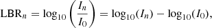
Methods. The evolution of the eruption and associated coronal dimming were analyzed using multiwavelength observations from the Atmospheric Imaging Assembly (AIA) and Hα observations from Kanzelhöhe Observatory. A detailed dimming analysis was performed based on an AIA 211 Å logarithmic base-ratio image sequence. To reconstruct the coronal magnetic field, we applied a physics-informed neural network (PINN)-based nonlinear force-free field (NLFFF) extrapolation method to a large computational volume (∼730 Mm × 550 Mm), using a pre-eruption photospheric vector magnetogram from the Helioseismic and Magnetic Imager (HMI) as the lower boundary.
Results. Our results show a highly asymmetric eruption. The eastern part of the filament erupts freely, creating a coronal dimming associated with its footprint, which subsequently expands (total area of ∼9 × 10⁹ km2) together with an inverse J-shaped flare ribbon. The eastern dimming area covers a weak magnetic field region with a mean unsigned flux of only ∼5 G. The NLFFF extrapolation shows the presence of a large-scale magnetic flux rope (MFR) of ∼500 Mm in length, consistent with the observed filament. We identified an extended MFR footprint to the east in the NLFFF extrapolation that connects to an inverse J-shaped flare ribbon (hook) observed during the eruption, outlining the area from which the coronal dimming originated. Overlying strapping fields connect to the region into which the coronal dimming and flare ribbon subsequently expand. This configuration offers a plausible explanation for the formation of the dimming as a stationary flux rope and strapping flux dimming. The subsequent expansion of the stationary flux rope dimming is caused by the growth of the MFR footprint through strapping-strapping reconnection. In contrast, the western filament leg shows multiple anchor points along a narrow channel and potentially strong overlying magnetic fields, which could have resulted in the suppressed dimming and partial confinement by overlying loops observed on this side of the filament during the eruption.
Conclusions. The reconstructed pre-eruptive NLFFF configuration provides a clear physical explanation for the observed asymmetries in the eruption, flare geometry, and coronal dimming. This successful application shows that PINN-based NLFFF extrapolation can be effective for modeling large-scale filaments extending into weak-field regions, and that combining this method with detailed observational analysis can greatly improve our understanding of complex solar eruptions.
Key words: Sun: corona / Sun: filaments / prominences / Sun: magnetic fields
© The Authors 2025
 Open Access article, published by EDP Sciences, under the terms of the Creative Commons Attribution License (https://creativecommons.org/licenses/by/4.0), which permits unrestricted use, distribution, and reproduction in any medium, provided the original work is properly cited.
This article is published in open access under the Subscribe to Open model. This email address is being protected from spambots. You need JavaScript enabled to view it. to support open access publication.
1. Introduction
Filaments are elongated structures of relatively cool and dense chromospheric plasma suspended in the hot corona (Parenti 2014) that form above polarity inversion lines (PILs). The observed filament material is generally believed to be located in the dips of sheared arcades or magnetic flux ropes (MFRs; for a review, see, e.g., Gibson 2018), as supported by magnetohydrodynamic (MHD) simulations (e.g., Hillier & van Ballegooijen 2013; Fan 2018). Some filaments can remain stable for several days or even weeks, while others undergo rapid changes and eventually erupt, thus causing coronal mass ejections (CMEs) and flares with potential space weather effects (see, e.g., review by Green et al. 2018). These eruptive events are often associated with coronal dimmings, which are regions with a strong transient decrease in emission caused by plasma evacuation along erupting field lines (Hudson et al. 1996; Sterling & Hudson 1997). The spatio-temporal evolution of dimmings offers important insights into eruption initiation, mass loss in the corona, and large-scale magnetic reconfigurations. Veronig et al. (2025) proposed a characterization of dimmings deduced from the spatio-temporal evolution of the dimming regions in relation to the flare ribbon evolution. This approach allows for the classification of the dimmings based on the magnetic flux systems involved in the eruption. Therefore, accurate reconstructions of the coronal magnetic field are essential, both for studying the magnetic structure and confinement of the filament itself and for correctly interpreting the various dimming signatures associated with its eruption.
The photospheric magnetic field in solar active regions (ARs) is measured with high accuracy by spectropolarimetric methods applied to polarization measurements. The Helioseismic and Magnetic Imager (HMI; Schou et al. 2012) on board the Solar Dynamics Observatory (SDO; Pesnell et al. 2012) represents a unique data source because it routinely measures photospheric polarization signals with high spatial and temporal resolution. Corresponding high-quality and high-cadence measurements of the coronal magnetic field vector remain elusive (for a recent review see Trujillo Bueno & del Pino Alemán 2022). Studies of the coronal magnetic field are therefore based on numerical approaches with different degrees of sophistication.
Data-constrained and data-driven MHD simulations are capable of describing the dynamic coronal evolution in a self-consistent way (see, e.g., the review by Jiang et al. 2022). These methods use the observed photospheric vector magnetic field data to initialize and guide the simulation, both in 3D space and time. The application of these methods allows us to study the slow (quasi-static) coronal evolution as driven by photospheric motions, the rapidly evolving field in solar eruptions, and the self-consistent transition between those states. Similar approaches have been extensively used to analyze the first X-class flare observed during solar cycle 24 (see, e.g., Afanasyev et al. 2023, for a recent work).
For studies that focus on the quasi-static pre- and post-eruptive corona, simpler approaches are used, for example nonlinear force-free field (NLFFF) models, which are also based on the photospheric vector magnetic field as input (for a review, see, e.g., Wiegelmann et al. 2017). NLFFF models are based on the assumption that the magnetic forces dominate the distribution of the plasma in the equilibrium corona. In other words, the plasma is assumed to be force-free, which means that the ratio of the gas to the magnetic pressure (called plasma-β) is small. The plasma-β model presented in Gary (2001) suggests that for a magnetic field that connects typical penumbral and plage regions, the force-free assumption may be justified at heights between ≈1.001 and 1.2 solar radii (≈2 to 40 Mm) when using β < 0.1 as a criterion. We note here that a value of β ≃ 0.1 is necessary to support prominences through magnetic tension (Hillier & van Ballegooijen 2013). The coronal height of 1.2 solar radii corresponds to altitudes at which the apexes of coronal loops in a potential state (i.e., having a more or less semicircular shape) typically reside. Values of β ≲ 0.01 may exist in the active-region corona between 1.001 and 1.01 solar radii (≈2 to 10 Mm; see Gary 2001)), i.e., below the height at which the magnetic structures that support filament material within ARs typically reside. Therefore, NLFFF methods have proven very successful in reconstructing MFRs that correspond well with observations of filament channels within ARs, i.e., with lengths of a few tens of megameters, located close to the main polarities, and oriented roughly along the main PIL, which typically exhibits strong transverse fields and magnetic shear (for a recent work, see, e.g., Thalmann et al. 2023). As elaborated in detail by Peter et al. (2015), a considerable scatter of plasma-β values may best characterize the AR corona, with the tendency to exhibit overall larger values at higher plasma temperatures, and with a median value of ≲0.1 (see their Fig. 1). They also examined the consequences of deviations from a force-free corona (characterized by β ≲ 0.01). In particular, NLFFF-based estimates of the (free) magnetic energy may be trustworthy only if the relative free energy (the ratio of the free to total energy) is substantially higher than the plasma-β.
Challenges are encountered when the NLFFF modeling is aimed at the reconstruction of MFR structures that are (partially) located outside of AR cores. Intermediate filaments connect the core to the periphery of ARs, while quiescent filaments are entirely located above quiet-Sun regions. As a consequence, one or both legs are located in weaker-field (≲100 G) regions so that the filaments may partially populate a coronal magnetic field that is not force-free. In the study of Rodríguez-Gómez et al. (2024), the plasma-β above quiet-Sun and coronal hole (CH) regions was studied based on a combination of observational data analysis and modeling. The plasma-β above the quiet Sun was found to lie well within the force-free range through the solar atmosphere outlined by Gary (2001). The non-force-free nature of a CH (β > 1) was also demonstrated by the observation-based study of Rodríguez-Gómez et al. (2024). The NLFFF modeling of partially non-force-free regimes can still be used to picture their basic connectivity. The weak-field magnetic field data poses a challenge as it adheres to a low signal-to-noise ratio. This is especially problematic for the transverse magnetic field, which often exhibits magnitudes close to the noise threshold of the instruments used. Motivated by and/or in correspondence with the uncertainty of the magnetic field measurements, adaptations of NLFFF methods (e.g, Wiegelmann et al. 2006, 2012; Wheatland & Régnier 2009; Mastrano et al. 2020) alter the observed field information (for a comparative study see DeRosa et al. 2015). In particular, the observed transverse field information is altered to a larger degree than that of the vertical field. As a consequence, attempts to reconstruct the sheared or twisted coronal field associated with filaments located away from the centers of ARs often fail.
Regarding the challenges outlined above, the physics-informed neural network (PINN; Raissi et al. 2019) approach, developed by Jarolim et al. (2023), appears advantageous. The method facilitates an intrinsic adjustment of the boundary condition (observed photospheric vector field) and allows for deviations from the physical model (NLFFF), where the solution is determined by the weighting between the two components. In this PINN-based method, the neural network finds a trade-off between the observational constraints and the physical NLFFF model, allowing it to avoid the use of manipulated (pre-processed) boundary data. In addition, the neural network acts as a neural representation of the magnetic field in the spatial simulation volume. This neural representation is key to efficiently storing the magnetic field information, and can provide valid extrapolations even for large simulation volumes (Purkhart et al. 2023, 2024). Instead of minimizing the Lorentz force and divergence in a volume-integrated form as traditional NLFFF models do (e.g., Wiegelmann et al. 2012), the method of Jarolim et al. (2023) trains iteratively, based on randomly sampled points from the simulation volume. In this way, it aims to find a force-free solution in the vicinity of each point within the computational volume, so that the solution may accommodate deviations from strict force-freeness where warranted by observational data, particularly in regions such as the quiet Sun or coronal holes where the photospheric magnetic field is weak.
This study investigates the eruption of a large-scale filament on February 24, 2023. While the central inverse S-shaped core of the pre-eruption filament structure was located within the strong magnetic fields of AR 13229, significant portions extended far into the surrounding weaker magnetic field regions on both its eastern and western sides, resulting in a total extent of the filament of ∼500 Mm. During the eruption, the eastern part of the filament appears anchored over a broad area in a weak field (plage) region, where a pronounced coronal dimming occurs later, indicating that the dimming is a core dimming occurring at the footprint of the erupting MFR. Notably, the total extent of this core dimming appears unusually large. The primary goal of this study is to understand the physical conditions underlying this asymmetric eruption, and in particular, the formation of such an extensive core dimming in a weak-field environment. We investigated the pre-eruptive magnetic connection between the filament/MFR and the coronal dimming region to gain insights into its formation and the underlying magnetic configuration. Given the challenges posed by this complex structure, we utilized the recently introduced PINN-based NLFFF extrapolation method NF2 (Jarolim et al. 2023) to reconstruct the pre-eruptive coronal magnetic field. This represents one of the few attempts (e.g., Jiang et al. 2014) to model large-scale filaments extending into weaker magnetic field regions outside the AR core.
2. Data and methods
2.1. Data
For the analysis of the filament eruption and associated flare, we utilized multiwavelength observations from the Atmospheric Imaging Assembly (AIA; Lemen et al. 2012) on board SDO (Pesnell et al. 2012) and ground-based Hα filtergrams from the Global Oscillation Network Group (GONG, Harvey et al. 1996) and the Kanzelhöhe Observatory for Solar and Environmental Research (KSO; Pötzi et al. 2021). The detailed coronal dimming analysis (see Sect. 2.2) specifically utilizes an image sequence from the AIA 211 Å channel and a line-of-sight (LOS) magnetogram from HMI (Schou et al. 2012). For context, we also used X-ray light curves observed by the Spectrometer/Telescope for Imaging X-rays (STIX; Krucker et al. 2020) on board Solar Orbiter (Müller et al. 2020).
We further used photospheric vector magnetic field data derived from full-disk polarization measurements from HMI. This data was processed as detailed in Sect. 2.3 to create the vector magnetogram that provides the lower boundary condition for our magnetic field extrapolation (see Sect. 2.4). Specifically, we utilized the 12 min cadence full-disk HMI data product (HMI.B_720s; Hoeksema et al. 2014) whose designated data slot time was 19:36 UT on February 24, 2023. The corresponding nominal observation time, as recorded in its FITS header, was approximately 19:34 UT and is used throughout this paper for comparison with AIA (extreme) ultraviolet ((E)UV) observations and Hα images from KSO.
2.2. Coronal dimming analysis
To characterize the evolution of the coronal dimming associated with the eruption, we performed a dimming analysis using the method described in Dissauer et al. (2018). Our analysis is based on a series of logarithmic base ratio (LBR) maps, calculated from the AIA 211 Å image sequence (2 × 2 pixel binning) as
 (1)
(1)
where In and I0 are pixel intensities in the AIA 211 Å images at the observation time tn and the base time t0 = 20:00 UT. A pixel in these LBR maps is then classified as a dimming pixel if its LBR intensity is below −0.5 log10 relative counts. All pixels marked as dimming pixels in one LBR map make up the instantaneous dimming mask for the corresponding observation time of that map (tn). The cumulative dimming mask is defined as all pixels that were considered part of a dimming at least once between t0 and tn. Finally, new dimming pixels are those that are considered dimming pixels for the first time at tn. We then derived a set of parameters from the instantaneous (inst) and cumulative (cumu) dimming mask sequences:
-
Icumu: the total LBR intensity at tn within the cumulative dimming mask from the end of the analyzed time interval (20:58 UT);
-
Acumu: the area of the cumulative mask at tn;
-
Φ−, cumu: the total negative flux in HMI LOS magnetogram pixels within the cumulative mask at tn;
-
Bunsigned, new: the unsigned magnetic flux density in new dimming pixels at tn.
2.3. HMI data processing
From the HMI.B_720s observables, total field strength, inclination, and the 180° ambiguity-corrected azimuth, we derive the image-plane magnetic field vector with a native (full-resolution) plate scale of ≈1 arcsecond. We retrieve the three photospheric vector magnetic field components (Bp, Bt, Br), where Bp, Bt, and Br refer to the phi (westward), theta (southward), and radial (out of photosphere) components of the magnetic field, respectively. These components are then remapped to local coordinates (Bx, By, and Bz, representing the horizontal and vertical magnetic field) using a cylindrical equal-area (CEA) transformation. We crop a rectangular submap in CEA coordinates with an extent of ∼720 × 540 Mm and centered on AR 13229. The area is bounded by four corners with the following Carrington coordinates: bottom left (357.6°,−1.2°), bottom right (52.5°,−1.2°), top right (64.8°,43.9°), and top left (345.3°,43.9°). We note that these Carrington coordinates only define the corners of the submap for reproducibility purposes, but the submap’s outline does not align with the Carrington longitudes and latitudes. This discrepancy occurs because CEA coordinates preserve a fixed pixel area, making the top and bottom boundaries of the submap equal in length (∼720). Consequently, when the rectangular submap in CEA coordinates is reprojected onto the full-disk observation (see Fig. 1), the contoured area appears to expand toward the north. The resulting vector magnetograms are analogous to space weather active region patches (SHARPs; Bobra et al. 2014), with a spatial sampling of 0.36 Mm, but are cropped over a larger field of view. This submap includes the filament under study, as well as its surroundings (see Fig. 1 and its discussion in Sect. 3.1).
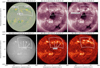 |
Fig. 1. Extent of the bottom boundary of the extrapolation volume (white contours; a rectangle in CEA coordinates) compared with selected full-disk observations before (first and second columns) and during the filament eruption (third column). The pre-eruption SDO/HMI LOS magnetogram and the SDO/AIA 211 Å and 304 Å images, match the time of our NLFFF extrapolation (19:34 UT). The KSO Hα image was recorded at 14:59 UT. |
Relative to the disk center, the lower boundary covers the photosphere in the approximate longitudinal range [−5°,50°] (from east to west), while the upper boundary covers it in the approximate range [−20°,70°]. The approximate latitudinal extent of the extrapolation volume is [55°,5°] (from north to south; see Fig. 1). The total filament complex and flare structure, which are the primary focus, are predominantly located between 0° and 50° in longitude. Gary & Hagyard (1990) demonstrated that in order to appropriately account for projection effects in the observed vector magnetic field data, the full spherical geometry must be taken into account for regions with angles greater than 50° away from the solar disk center. Since the outermost edges of the covered photospheric domain extend to approximately 70° in the top right corner, the Cartesian grid-based extrapolation used in this study may introduce inaccuracies in these peripheral areas of the extrapolation volume. However, since the filament of interest lies fully within the 50° limit, we consider our methodology suitable for focusing on this specific structure. We acknowledge, however, that this Cartesian approach has inherent shortcomings, particularly for accurately modeling coronal features that extend into significantly foreshortened regions or those that occupy a large fraction of the spherical coronal volume. The application of PINN-based NLFFF extrapolations within a spherical geometry will be explored in future work to address these limitations.
2.4. PINN-based NLFFF extrapolation
For the 3D coronal magnetic field modeling, we applied the NLFFF extrapolation method by Jarolim et al. (2023) (NF2) to a computational volume with an extent of ∼720 × 540 × 300 Mm. Specifically, we used the extrapolations based on the vector potential, which were introduced in Jarolim et al. (2024a). The approach is based on a PINN (Raissi et al. 2019), where the neural network acts as a mesh-free representation of the simulation volume, mapping coordinate points (x, y, z) to the respective magnetic field vector B = (Bx, By, Bz). The neural network is optimized to provide a solution to the boundary-value problem, where the bottom boundary corresponds to the observed vector magnetogram, and the side and top boundaries are approximated by a potential field solution. The system of coupled partial differential equations is given by the divergence-free ∇ ⋅ B = 0 and force-free J × B = (∇×B)×B = 0 equations. Here J refers to the magnetic current density.
For this study we used the vector potential implementation, where the output of the neural network B is replaced with the vector potential A = (Ax, Ay, Az). The magnetic field is then computed by B = ∇ × A. Therefore, the divergence-free condition is directly satisfied through the fundamental vector calculus identity ∇ ⋅ B = ∇ ⋅ (∇×A) = 0, and the problem reduced to the force-free and boundary conditions.
The algorithm iteratively samples 8192 coordinate points from the bottom and lateral potential boundary conditions and 16384 points randomly from within the simulation volume. It updates the neural network to minimize both the deviation from the boundary condition and the physical constraints. During each updating step, we minimize the residuals of the force-free loss
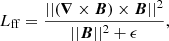 (2)
(2)
where ∥B∥2 is used for the scaling of the loss term and ϵ = 10−7 is added for numerical stability. In addition, we minimize the deviation from the observed magnetic field B0(x, y)
 (3)
(3)
We further account for uncertainties in the measurement Berror by subtracting the error map and only optimizing points that exceed the error threshold
 (4)
(4)
For the boundary loss, we then compute the vector norm of the clipped difference vector
 (5)
(5)
Analogously, we compute the difference to the potential boundary condition, where we optimize the deviation from the precomputed potential field Bpotential(x, y, z) at the side and top boundaries
 (6)
(6)
The total loss is then given by
 (7)
(7)
where the λ parameters refer to the weighting of the force-free loss λff, boundary loss λB0, and potential boundary loss λpotential.
We optimize the neural network for 200 000 iterations until we reach convergence. The weighting factor of the boundary condition λB0 is decayed from 1000 to 1 over 50 000 iterations. This enables an initial emphasis on the boundary condition, achieving, in general, a better agreement between the observational data and the physical model. The weighting factor for the potential boundary condition is fixed to λpotential = 1 throughout this work. The force-free weighting factor λff is set to 0.4 over the full training.
We conducted a sensitivity analysis of the NLFFF results using different force-free weighting factors λff (see Appendix A). Overall, the individual extrapolations yield similar magnetic field solutions, and all contain a high-current density channel made up of an MFR that corresponds to the filament. The main differences between the different extrapolations are the continuity of the MFR and the magnetic structures associated with the southernmost part of the coronal dimming region. Despite these variations, all solutions support the same interpretation of the observed event. We find that a weighting factor of λff = 0.40 for the force-free condition yields the best match with observations and produces robust quantitative metrics.
The specific advantage of this approach is the memory and computational efficiency, which enables the extension to large computational volumes, capturing both small- and large-scale features. For example, the mesh-free representation can efficiently encode a highly twisted MFR, overcoming limitations due to numerical discretization, while simultaneously capturing the global topology of the AR. This can also be seen from the compression factor, where the neural network weights require ∼60 times less storage than the corresponding grid-based representation.
For the visualization of our results, we converted the neural representation to a grid representation by sampling our simulation volume at a resolution of 0.72 Mm per pixel. This corresponds to a rebinning by a factor of two from the resolution of the original HMI data, which is necessary due to memory limitations. We note that the discretizations can result in residual terms of the divergence-freeness, while the function representation of the neural network is, by definition, divergence-free to the level of numerical accuracy. For the computed metrics, deviations occur depending on the sampled resolution; however, all metrics show only minor variations or are below target threshold values (see Sect. 3.3). For the sensitivity study described in Appendix A, we reduced the spatial sampling by a factor of four (1.44 Mm) to accommodate the data volume.
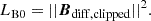
To quantify the force-free consistency of the NLFFF modeling, we used the current-weighted angle between the modeled magnetic field and electric current density (Schrijver et al. 2006) as a measure. Here we find θj ≃ 17°, which indicates that, on average, the electric currents deviate less than ≈17° from the magnetic field aligned direction (ideally, θj = 0). Second, the energy contribution that arises from the nonsolenoidal component of the magnetic field (Ediv), i.e., the contribution due to the violation of ∇ ⋅ B = 0, has to be small compared to the total NLFFF energy (for details, see the in-depth study of Valori et al. 2013). In the dedicated study by Thalmann et al. (2019), an upper limit of 5% was suggested for solar applications to guarantee a reliable helicity computation. In this study we find a contribution of Ediv < 1%.
The resulting NLFFF extrapolation was visualized using the open-source software ParaView1. Reprojections of the AIA and KSO observations to the bottom boundary of the extrapolation volume in CEA projection and general visualization of these results were performed using version 5.0.0 (Mumford et al. 2023) of the SunPy open-source software package (The SunPy Community et al. 2020).
3. Results
3.1. Event overview
In Fig. 1 we relate the extent of our extrapolation volume to full-disk observations of HMI, AIA, and KSO before and during the filament eruption and flare. Specifically, the contours outline the extent of the HMI vector magnetogram used as the bottom boundary in our extrapolation (see Sect. 2.3). AR 13229, which contains the filament of interest, is located in the northwest quadrant of the solar disk. It was classified as a β magnetic field configuration by the National Oceanic and Atmospheric Administration (NOAA) Active Region Summary2 and as an E-type sunspot configuration by the KSO3 on the day of these observations.
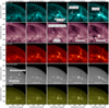 |
Fig. 2. Overview of the filament eruption and associated M3.7 flare as observed in selected SDO/AIA channels and GONG Hα filtergrams. The figure is adapted from Purkhart et al. (2025). The movie accompanying this figure shows the full eruption in more wavelength channels. The associated movie is available online. |
The KSO Hα image shows the pre-eruption filament at 14:59 UT, which was the last observation of the day. It was used in this study for comparison with the NLFFF extrapolation results because of its superior sharpness instead of an Hα image from GONG, which could have matched the extrapolation time exactly. This is especially useful when comparing smaller-scale details in later figures. The central inverse S-shaped part of the filament appears most prominent. In addition, a thinner, approximately east–west aligned filament segment extends farther to the east, which appears separated from the central filament. The western extension of the inverse S-shaped filament does not appear continuous, but in the form of several dark patches. A very similar filament structure can also be seen in the AIA 304 Å image closer to the time of the eruption (19:34 UT).
The filament was observed to survive several (partial) filament eruptions during the disk passage of AR 13229. An in-depth study of the X2.3 flare and CME on February 17 is presented in Ahamed et al. (2025) and of the M6.4 flare and filament eruption on February 25 is presented in Song et al. (2024). For completeness, we note that the filament eruptions occurred during the decaying phase of AR 13229 from early February 22 to late February 25 (analyzed in detail by Idrees et al. 2024). Our NLFFF extrapolation focuses on the pre-event state of the February 24, 2023, filament eruption and the associated M3.7 flare. We note that the filament eruption under study was associated with a fast halo CME with a speed of ∼1300 km/s, as listed in the SOHO/LASCO CME catalogue4, and an interplanetary CME (ICME) measured in situ by Wind on February 27, 2023 (Richardson & Cane ICME catalog5). The extrapolation time (19:34 UT) was chosen to be about 30 min before the onset of the GOES flare at 20:03 UT and about one hour before its soft X-ray peak time at 20:30 UT. The AIA 211 Å and 304 Å filtergrams at 20:35 UT in Fig. 1 show the flare ribbons that span essentially the full extent of the pre-eruption filament. In addition, the strong coronal dimming region east of the flare loop arcade is clearly visible. The flare was analyzed in detail by Purkhart et al. (2025), who focused in particular on the spatio-temporal evolution of quasi-periodic UV and X-ray pulsations.
The extent of the extrapolation volume was chosen to include the main features of the filament and flare. It covers much of the visible northern hemisphere (Fig. 1, white outline; ∼720 Mm × 540 Mm). It fully includes AR 13229 with the filament of interest, as well as the smaller AR 13235 to the west, part of the coronal hole close to the disk center, and part of a polar coronal hole. AR 13234 in the east is not included.
Figure 2 gives an overview of the filament eruption and flare in multiple SDO/AIA wavelength channels and GONG Hα observations, highlighting the key features. The event is discussed in much more detail by Purkhart et al. (2025), from where this figure is adapted. The accompanying movie shows the sequence of observations over the entire event. In the pre-eruption images (e.g., 19:51 UT), both the central inverse S-shaped portion and the eastern straight portion of the overall filament structure can be seen. The key observation relevant to this study is that the subsequent filament eruption and flare were strongly asymmetric. The filament eruption can be characterized as a whipping-like type (Liu et al. 2009), with an active eastern leg and an anchored western leg. The footprint of the active eastern leg is initially surrounded by an inverse J-shaped flare ribbon structure (e.g., AIA 304 Å frame at 20:17 UT). This inverse J-shaped ribbon grows away from the PIL until finally the hook of the ribbon opens up completely by rapidly moving to the east (see the AIA 304 Å image sequence). A coronal dimming region forms within the area outlined by this inverse J-shaped ribbon and then expands following the motion of the flare ribbon (e.g., compare the 20:25 UT and 20:43 UT frames in AIA 211 and 304 Å). Part of the straight filament channel, which extends along the northern part of this inverse J-shaped ribbon, does not erupt and is injected with hot plasma during the event (see, e.g., movie or frames at 20:25 UT). The anchored western filament leg is confined by a hot overlying loop system (e.g., AIA 131 Å frame at 20:43 UT) and remains attached to the Sun throughout the impulsive phase of the flare until about 20:43 UT. The flare ribbon structure along the confined western filament leg appears more patchy and not as well-defined as the inverse J-shaped ribbon in the east.
3.2. Coronal dimming
Figure 3 and the accompanying movie give an overview of the evolution of the coronal dimming. While the AIA 211 Å image sequence qualitatively shows the strong asymmetry of the filament eruption and the coronal dimming, the LBR maps allow a quantitative investigation into the temporal and spatial evolution of the dimming. The LBR maps clearly illustrate that the coronal dimming associated with the footprint of the eastern filament leg is by far the most pronounced dimming observed in this region in terms of brightness decrease (see bottom panel at 20:48 UT).
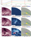 |
Fig. 3. Evolution of the coronal dimming associated with the filament eruption. Upper panel: Time series of STIX counts in three different energy bands. The selected observation times are marked by the red vertical lines. Bottom panels: Selected observation times. Each row corresponds to one time and shows the AIA 211 Å image from that time, the derived LBR map (the base time is 20:00 UT) with instantaneous and cumulative dimming masks (threshold: LBR = −0.5 log10 relative counts), and the HMI LOS magnetogram from 20:00 UT with the same dimming mask contours. The associated movie is available online. |
There is a faint darkening in the central part of the map detected by the LBR maps (white area). This is the region over which the filament moves during the eruption, and the dark filament plasma causes numerous false detections in this region. Other parts appear to be caused by the motion of loops in the surrounding region. However, the filament eruption also creates a valid dimming signature in this region, in the sense that the broader filament structure and the loops above it have erupted and no longer contribute to the emission along this LOS. However, this is not the dimming we are interested in, so we set the threshold (−0.5 log10 relative counts) of the dimming mask low enough to mainly capture the evolution of the strongest dimming in the east.
The dimming mask sequence clearly shows how the eastern coronal dimming of interest starts within the area outlined by the original inverse J-shaped flare ribbon (20:21 UT), further highlighting the connection of the eastern leg of the erupting filament to the dimming and supporting its classification as a core dimming. The initial dimming subsequently quickly expands farther to the southeast, while the hook of the inverse J-shaped ribbon opens up by following the expansion of the dimming. Later during the event (e.g., 20:48 UT), the remaining straight section of the (originally inverse J-shaped) flare ribbon appears to move from the north into the previous dimming region. This is especially evident from the difference between the instantaneous and cumulative dimming masks at this time. Comparison of the dimming masks with the HMI LOS magnetogram shows that the final dimming region covers a large part of the negative polarity magnetic field region outside the main part of the AR.
Figure 4 shows the dimming mask evolution and the derived parameters specifically for the subarea around the eastern dimming region. The cumulative dimming intensity (Icumu) decreases rapidly during the impulsive phase of the flare between approximately 20:17 UT and 20:30 UT (for reference, see the STIX 15–25 keV light curve) and then continues to decrease more slowly until about 20:50 UT. At the end of the analyzed time interval, the dimming intensity is already increasing again, as indicated by the positive derivative.
 |
Fig. 4. Time evolution of the cumulative dimming mask and the extracted parameters of the major dimming region associated with the footprint of the eastern filament leg. Top panel: HMI LOS magnetogram with the dimming mask. The pixels are color-coded according to the time they were first classified as a dimming pixel (threshold: LBR = −0.5 log10 relative counts). Bottom panels: Time evolution of dimming parameters (black). From top to bottom: Cumulative intensity (Icumu), cumulative area (Acumu), cumulative negative flux (Φ−, cumu), and new unsigned magnetic flux density (Bunsigned, new). The time evolution of the derivative of each quantity is shown in blue. The STIX 15-25 keV light curve (green) is included in each panel as a reference. |
Our analysis also captures most of the expansion of the dimming. The cumulative dimming area (Acumu) expands most rapidly during the impulsive phase of the flare, with the area growth rate characterized by three prominent peaks that show some similarity to the STIX hard X-ray light curve. After the impulsive phase, the derivative of the cumulative area decreases sharply. The cumulative dimming mask reaches a final area of 9.25 × 10⁹ km2 (all colored pixels in the top panel).
The total negative magnetic flux (Φ−, cumu) within the final cumulative dimming area is −7.93 × 10²⁰ Mx. Its growth rate is closely related to the area growth rate. However, instead of three major peaks, it has only two peaks because stronger magnetic regions were covered during the later two peaks compared to the first, as can be seen in the unsigned magnetic flux density (Bunsigned, new). The unsigned magnetic flux density of the newly added dimming pixels remains quite low (∼2.5–12.5 G) throughout the event. The mean unsigned magnetic flux density within the final cumulative dimming mask is only 5.2 G.
3.3. Coronal magnetic field modeling results
Figure 5 shows an overview of our NLFFF extrapolation along with observations reprojected to the same CEA coordinate frame. The HMI Br magnetogram (panel a) provides further insight into the magnetic configuration of AR 13229. An inverse S-shaped PIL (indicated by the green dotted line) separates the two major polarity regions in the core of the AR. The same PIL extends farther into the surrounding weaker magnetic regions on either side. In addition, the contours show the full extent of the flare ribbons along both sides of the PIL, as observed in the AIA 1600 Å channel over the course of the flare. The brightest parts of the flare ribbons lie parallel to each other on either side of the PIL. The much fainter inverse J-shaped ribbon extends eastward into the negative magnetic polarity associated with the dimming. The full extent is indicated by the white dashed line (compare with the observations in Fig. 1). The northern flare ribbon extends farther toward the west along the inverse S-shaped PIL. It is partially connected to the two sunspots, but also extends farther along the PIL into weaker magnetic field regions.
 |
Fig. 5. Overview of NLFFF extrapolation results and comparison with observations reprojected to the CEA coordinate frame of the extrapolation. (a) HMI Br magnetogram. The contours show the maximum brightness of flare ribbons in a series of AIA 1600 Å images between 20:00 and 20:45 UT. The contour levels are 25, 100, and 400 DN/s. (b) 5000 field lines randomly started from the lower boundary of the extrapolation volume with the HMI LOS magnetogram and AIA 1600 Å contours as background. The field lines are color-coded according to the local current density. Regions of low current density are made increasingly transparent to keep the underlying high current density filament channel visible. (c) Same as b, but with 50 000 field lines. (d) 5000 field lines with the AIA 211 Å image showing the dimming as a background. The dimming area is marked by a cyan mask. (e and f) reprojected KSO Hα and AIA 211 Å images for reference. The locations of the PIL (green dotted) and inverse J-shaped flare ribbon (white dashed) are indicated on some panels. The movie accompanying this figure shows a smooth transition between the NLFFF extrapolation and the AIA 304 Å and KSO Hα images. The movie is available online. |
The close-up of the Hα image from KSO (panel e) shows the fine structure of the filament channel discussed earlier: a thick inverse S-shaped filament channel in the center, a straight channel in the east, and several filament fragments in the west. The central inverse S-shaped section appears shifted with respect to the PIL, while the other sections, especially the eastern portion, are co-aligned with the PIL. A comparison with the AIA 304 Å image (panel f) confirms that the filament has remained largely unchanged in the four hours between the two observations. The only notable difference is that the inverse S-shaped part has moved slightly farther away from the PIL, which we interpret as an increase in the height of this central part. This effect can also be observed during the onset of the eruption at about 20:00 UT in the movie accompanying Fig. 1. This motion also reinforces the impression of a separation between the central filament and the straight eastern channel. The western part of the filament appears as a slightly more continuous structure in AIA 304 Å with an apparent discontinuity that roughly coincides with the end of the drawn PIL.
The two visualizations of the magnetic field lines (panels b and c) give an overview of the associated model magnetic field configuration. For this purpose, field lines were randomly sampled from the lower boundary of the extrapolation volume. They are colored according to the local current density. Yellow represents the highest current density and blue indicates low current density. A channel of high current density is visible; its length and shape closely match the filament structure in the AIA and KSO observations. The movie accompanying the figure allows a detailed comparison between the NLFFF model and the observations by smoothly blending the two. The central part of the high current density channel follows the PIL much closer than the observed filament, so the inverse S-shaped portion of the strong current density channel also appears less curved.
Field lines overlying the eastern filament leg (called the strapping field) are anchored in the weak magnetic field regions on either side of the PIL (panel b of Figure 5). Their footprint in the negative magnetic polarity region coincides closely with the southern boundary of the observed dimming region (panel d). On the other hand, the strapping field in the west is partially anchored in much stronger magnetic field regions close to the sunspots.
From our NLFFF modeling, we estimate a pre-eruption, free magnetic energy of ≈3 × 1032 erg. The sign of the derived total magnetic helicity (≈ − 4.9 × 1043 Mx2) is in agreement with the inverse S-shaped part of the filament. We note that this is also in agreement with the hemispheric sign preference, i.e., negative helicity in the northern and positive helicity in the southern hemisphere of the Sun (cf. Martens & Zwaan 2001).
Figure 6 shows the structure of the NLFFF filament channel in more detail, focusing in particular on its relationship to the straight eastern part of the filament, the inverse J-shaped flare ribbon, and the coronal dimming region. We find that field lines starting from the easternmost extension of the observed filament form the compact core of the MFR in our NLFFF extrapolation (left column). This MFR closely follows the PIL to the east, matching the position of the eastern straight filament channel in the pre-flare observations (AIA 304 Å and KSO Hα) and the heated channel during the flare (AIA 211 Å). The compact MFR continues to strictly follow the inverse S-shaped part of the PIL into the western region. At its western end, it forms an unexpected loop.
 |
Fig. 6. Field lines associated with the core of the MFR (left column), the inverse J-shaped ribbon (middle column), and the coronal dimming region (right column). The field lines start from a single circular seed source at the eastern end of the shown structure (left column); from multiple circular seed sources covering the area inside the inverse J-shaped ribbon, as suggested by the maximum AIA 1600 Å contours (middle column); and from inside the dimming region, as determined by all pixels below the threshold of −0.5 in the logarithmic AIA 211 Å base ratio image of 20:35 UT (see Sect. 3.2 for more details). Each field structure is compared with the HMI Br magnetogram from the NLFFF extrapolation time (top row). Side views from the direction of the colored arrows (red and blue) are shown in the insets. The cyan line roughly indicates the extent of the main part of the flare ribbons. The field structures are compared with the AIA 211, 304 Å, and KSO Hα observations. The dimming mask used as a seed source is shown in the inset of the AIA 211 Å observation. |
Most of the field lines starting from the area surrounded by the inverse J-shaped ribbon (middle column) also become part of the MFR. They do so by first arching over the straight MFR core and then wrapping tightly around it, forming the wider part of the MFR (see also the insets showing side views in the upper panel). A comparison with KSO Hα shows how this structure envelops the eastern straight filament channel and how the apparently looser winding of the field lines starts roughly at the western end of the straight filament channel. The resulting wider MFR structure also matches the western part of the filament with its discontinuity (AIA 304 Å and KSO Hα). A comparison with the AIA 211 Å image shows how the footprint of this MFR covers the northern part of the dimming region initially enclosed by the inverse J-shaped ribbon and identified as the filament’s anchoring region in the AIA observations during the eruption (see Fig. 2).
The field lines starting from the dimming region, as observed in AIA 211 Å at 20:35 UT (right column), show that the remaining dimming region around the inverse J-shaped ribbon (compare with top panel) is associated with loops that lie directly above the MFR, acting as a strapping field (see side view in blue box). Our NLFFF extrapolation therefore suggests that the larger coronal dimming region beyond the inverse J-shaped ribbon was not connected to the MFR before the eruption.
The magnetic structure of the filament’s western leg is much more compact, meaning its connection to the solar surface does not spread out over a wide area. However, some intermediate connections to the lower extrapolation boundary are visible, most notably a connection toward the sunspots.
The side views of each structure discussed (top panels, red box) show their height profiles. The filament core (left column) reaches a height of about 60 Mm (excluding the loop at its western end), with a local minimum of about 45 Mm between the main parts of the two flare ribbons. The filament structure associated with the inverse J-shaped flare ribbon (middle column) further shows that the central part of the MFR has the lowest altitude in our NLFFF model. The extended anchoring structure of the eastern leg reaches a height of about 60 Mm, and the overlying loop system connected to the dimming region (right column) reaches a height of over 100 Mm.
4. Discussion
Our multiwavelength observations reveal a complex eruptive event with strong asymmetries. The filament eruption occurred in a whipping-like manner: the eastern leg erupted freely, while the western leg remained partially confined. This asymmetry was mirrored in the flare ribbons and, most prominently, in the resulting coronal dimming. The eastern dimming, closely associated with the anchor point of the eastern filament leg in observations (which identifies it as a core dimming), is by far the most pronounced dimming in terms of brightness decrease. Compared to the dimming population analyzed in the statistical study of Dissauer et al. (2018), the derived characteristic parameters such as area, area growth rate, intensity, and magnetic flux fall within the ranges typically observed for overall dimmings (i.e., the combination of core dimmings interpreted as the footprint of MFRs and the more widespread secondary dimmings). However, we note that the mean unsigned magnetic flux density within the extended eastern dimming area (∼5 G) is considerably lower than in the dimming population from Dissauer et al. (2018), who found that the mean unsigned magnetic flux density mostly lies in the range of 25–150 G. The low magnetic flux densities in the event under study are consistent with the dimming’s location at the eastern filament anchor point, situated at the periphery of an AR, predominantly in regions of weak magnetic fields.
To interpret these observations and to investigate the underlying magnetic drivers, we relate them to the pre-flare NLFFF magnetic field extrapolation. The PINN-based NLFFF extrapolation method has successfully reconstructed the pre-eruptive magnetic field of the complex large-scale (∼500 Mm) filament, showing good overall consistency with the observed filament complex in the SDO/AIA EUV and KSO Hα images. A closer inspection (see Fig. 6) reveals a NLFFF filament channel with significant east–west asymmetry. While the core of the modeled MFR spans the full extent of the filament toward the east, the field lines forming the outer parts of the MFR fan out into an extended structure connected to the eastern weaker-field region. In contrast, the western part of the NLFFF filament consists mainly of the narrow MFR with potentially several intermediate anchor points, particularly to the stronger field region near the sunspots.
In addition to the filament channel, our NLFFF model reveals the overlying fields along the filament, with potentially stronger overlying fields connected to the sunspots along its western leg (see Fig. 5, panel b). Coupled with the multiple anchor points identified in the NLFFF model for the western filament leg, this could contribute to stronger magnetic confinement of the western part of the erupting filament. This is consistent with the observed asymmetric eruption, which is characterized by a freely escaping eastern filament leg and a more anchored western leg, partially confined by hot overlying loops (see Fig. 2).
The extended eastern filament footprint in the NLFFF naturally explains the formation of the observed inverse J-shaped flare ribbon in the east, consistent with the imprint of quasi-separatrix layers (QSLs) around MFR anchor points. This is a central feature of the standard flare model in 3D (Démoulin et al. 1996; Janvier et al. 2014) and was discussed in much detail for this particular flare in Purkhart et al. (2025). In contrast, the western filament leg with its multiple anchor points in the model corresponds well with the more patchy flare ribbon observed in the west. The asymmetric filament eruption and the asymmetric filament footprints also resulted in the strong asymmetry of the dimming signatures (see Fig. 3). The freely escaping eastern filament leg with its large footprint resulted in the pronounced dimming, while the plasma outflow through the confined narrow western leg largely suppressed the formation of dimming on this side.
The magnetic connectivity of the eastern dimming region revealed by our extrapolation allows us to interpret the dimming in terms of the physics-based categorization introduced by Veronig et al. (2025). The dimming is initially formed within the area outlined by the inverse J-shaped flare ribbon, which is directly connected to the fanned-out footprint of the MFR in our NLFFF extrapolation (see Fig. 6, middle column). This connection clearly identifies the dimming as a flux-rope dimming, equivalent to the concept of a core dimming. The initial growth of the inverse J-shaped ribbon and the dimming into the surrounding area associated with the overlying strapping fields (see Fig. 6, right column) is consistent with the stationary flux rope and strapping flux dimming categories. In this scenario, additional flux can be added to the erupting MFR via strapping-strapping reconnection of the overlying fields, resulting in the expansion of the MFR footprint and, consequently, the dimming into the strapping flux region.
The subsequent more rapid growth of the dimming starting around 20:25 UT (see also the derivative of Acumu in Fig. 4) coincides with the rapid opening of the flare ribbon’s hook. This continued simultaneous expansion of the ribbon and dimming indicates further reconnection of the strapping flux. At about the same time, the much slower apparent movement of the northern straight part of that flare ribbon into the established dimming area becomes visible (see also the difference in the instantaneous and cumulative dimming masks in Fig. 3). This indicates the onset of the direct involvement of the flux rope in the reconnection process. Therefore, this phase could at least partially be considered a moving flux-rope dimming driven by rope-strapping reconnection.
While these categories are idealized, they give a good idea of how the dimming may have evolved with respect to the magnetic flux systems involved in the eruption. More importantly, they illustrate that our NLFFF model represents a realistic pre-eruptive MFR and overlying arcade configuration that allows for the formation of a coronal dimming in this area during the eruption.
Differences between the extrapolation and the observations are apparent for the central inverse S-shaped part of the filament. Here, the observed filament is displaced in relation to the model MFR (see Fig. 6). In addition, the central inverse S-shaped part of the filament seems to be slightly separated from the straight eastern filament channel in the observations. This visual impression of two separate filament channels greatly increases during the onset of the eruption, where the eastern end of the inverse S-shaped part slides along the eastern straight filament channel (see, e.g., GONG Hα in the movie accompanying Fig. 2). However, the observation of hot plasma injection into the eastern straight channel during the flare (see Fig. 2) strongly indicates that a significant magnetic connection between these filament sections persisted until the eruption.
We recall here that the deviation between the model magnetic field and the observations may be of different origins, including projection effects, dynamic evolution, and, above all, the deviation of the real corona from a force-free state (i.e., plasma-β not small, in contrast to the very basic assumption of NLFFF modeling). Also outside the strong core field of AR 13229, our NLFFF model successfully reproduces the observations in essence, including the connectivity to a remote coronal dimming area. Thus, while our NLFFF might depict a somewhat idealized model, it effectively captures the essential large-scale connectivity and provides insights into the observed asymmetries in the filament eruption, flare geometry, and the associated coronal dimming.
While some deviation from the observations is always to be expected from an NLFFF extrapolation, we conclude that our extrapolation captures key features of the pre-eruptive filament structure, suggesting that the PINN-based method of Jarolim et al. (2023) performs well even under such challenging conditions. This success may be attributed to specific advantages of PINNs (highlighted in Sects. 1 and 2.4), including their intrinsic capability to find a trade-off between observational boundary conditions and the physical NLFFF model, potentially mitigating issues from noisy or weak-field data without explicit pre-processing. In addition, the mesh-free representation and efficient handling of large extrapolation volumes are crucial for modeling such extensive structures.
While our study demonstrates promising results for the application of this method for very extended filaments and weak field regions, future studies could perform more systematic comparisons of the PINN-based approach with other methods. Furthermore, this method could also be tried on quiescent filaments without any connection to an AR to see if the limit of NLFFF extrapolation capabilities can be pushed even further. Photospheric vector magnetograms provide limited constraints for magnetic field extrapolations. Therefore, incorporating chromospheric measurements, as already demonstrated (Jarolim et al. 2024b), could improve the results, especially for challenging cases such as large-scale filaments. In addition, a global implementation of this method may be advantageous.
5. Conclusion
In this study we analyzed the asymmetric eruption of a ∼500 Mm filament on February 24, 2023, and identified potential magnetic drivers for the observed phenomena using a PINN-based NLFFF extrapolation. A key feature of this event was the formation of a prominent coronal dimming around the eastern anchor point of the erupting filament. The dimming started within the area outlined by an inverse J-shaped flare ribbon before rapidly expanding to a final area of ∼9 × 10⁹ km2 with a mean unsigned flux of only ∼5 G. Our NLFFF extrapolation suggests the presence of a large MFR with an extended eastern footprint located within the initial dimming region. The model also suggests that the area into which the dimming expanded is connected to strapping field lines that overlay the MFR’s extended eastern leg. This configuration provides a realistic scenario for the formation and evolution of the coronal dimming during the eruption. According to the categories introduced by Veronig et al. (2025), the dimming can be described as a stationary flux-rope dimming and strapping flux dimming. The area of the stationary flux-rope dimming initially increases due to strapping-strapping reconnection, which adds more flux to the MFR and consequently expands its footprint. The later apparent motion of the flare ribbons into the established dimming region indicates a transition to a moving flux-rope dimming, driven by rope-strapping reconnection. In contrast, the western filament leg shows multiple anchor points and a potentially stronger overlying magnetic field in the NLFFF extrapolation, which may have contributed to the asymmetric confinement and the lack of significant dimming in that area.
Reconstructing the magnetic structure of large filaments, especially those extending into regions with weak magnetic fields, is challenging for NLFFF extrapolation methods. The PINN-based approach by Jarolim et al. (2023) used here may have specific advantages for such cases compared to traditional methods. Despite the challenging configuration of the filament and the overall complexity and size of the extrapolation volume (∼720 Mm × 540 Mm), the method successfully reconstructed a filament structure consisting of a ∼500 Mm MFR that is consistent with the filament channel observed in KSO Hα and AIA EUV observations and offers a plausible scenario for the evolution of key observations such as the coronal dimming. While this study presents only a single event, it demonstrates the potential of PINN-based NLFFF extrapolation to model large-scale filaments connecting to weak-field regions and to provide insights into the magnetic drivers behind their eruptions.
Data availability
Movies associated with Figs. 2, 3, 5 are available at https://www.aanda.org
Acknowledgments
This research was funded in part by the Austrian Science Fund (FWF) 10.55776/I4555 and 10.55776/PAT7894023. This project has received funding from the European Union’s Horizon Europe research and innovation programme under grant agreement No 101134999 (SOLER). Views and opinions expressed are however those of the author(s) only and do not necessarily reflect those of the European Union and therefore the European Union cannot be held responsible for them. Solar Orbiter is a space mission of international collaboration between ESA and NASA, operated by ESA. The STIX instrument is an international collaboration between Switzerland, Poland, France, Czech Republic, Germany, Austria, Ireland, and Italy. Hα data were provided by the Kanzelhöhe Observatory, University of Graz, Austria. Data were acquired by GONG instruments operated by NISP/NSO/AURA/NSF with contribution from NOAA.
References
- Afanasyev, A. N., Fan, Y., Kazachenko, M. D., & Cheung, M. C. M. 2023, ApJ, 952, 136 [Google Scholar]
- Ahamed, A. A., Subramanian, S. P., Rahman, A. M., et al. 2025, New Astron., 114, 102312 [Google Scholar]
- Bobra, M. G., Sun, X., Hoeksema, J. T., et al. 2014, Sol. Phys., 289, 3549 [Google Scholar]
- Démoulin, P., Priest, E. R., & Lonie, D. P. 1996, J. Geophys. Res., 101, 7631 [Google Scholar]
- DeRosa, M. L., Wheatland, M. S., Leka, K. D., et al. 2015, ApJ, 811, 107 [NASA ADS] [CrossRef] [Google Scholar]
- Dissauer, K., Veronig, A. M., Temmer, M., Podladchikova, T., & Vanninathan, K. 2018, ApJ, 863, 169 [NASA ADS] [CrossRef] [Google Scholar]
- Fan, Y. 2018, ApJ, 862, 54 [Google Scholar]
- Gary, G. A. 2001, Sol. Phys., 203, 71 [Google Scholar]
- Gary, G. A., & Hagyard, M. J. 1990, Sol. Phys., 126, 21 [Google Scholar]
- Gibson, S. E. 2018, Liv. Rev. Sol. Phys., 15, 7 [Google Scholar]
- Green, L. M., Török, T., Vršnak, B., Manchester, W., & Veronig, A. 2018, Space Sci. Rev., 214, 46 [Google Scholar]
- Harvey, J. W., Hill, F., Hubbard, R. P., et al. 1996, Science, 272, 1284 [Google Scholar]
- Hillier, A., & van Ballegooijen, A. 2013, ApJ, 766, 126 [Google Scholar]
- Hoeksema, J. T., Liu, Y., Hayashi, K., et al. 2014, Sol. Phys., 289, 3483 [Google Scholar]
- Hudson, H. S., Acton, L. W., & Freeland, S. L. 1996, ApJ, 470, 629 [CrossRef] [Google Scholar]
- Idrees, S., Su, J., Chen, J., & Deng, Y. 2024, Sol. Phys., 299, 91 [Google Scholar]
- Janvier, M., Aulanier, G., Bommier, V., et al. 2014, ApJ, 788, 60 [Google Scholar]
- Jarolim, R., Thalmann, J. K., Veronig, A. M., & Podladchikova, T. 2023, Nat. Astron., 7, 1171 [NASA ADS] [CrossRef] [Google Scholar]
- Jarolim, R., Veronig, A. M., Purkhart, S., Zhang, P., & Rempel, M. 2024a, ApJ, 976, L12 [Google Scholar]
- Jarolim, R., Tremblay, B., Rempel, M., et al. 2024b, ApJ, 963, L21 [NASA ADS] [CrossRef] [Google Scholar]
- Jiang, C., Wu, S. T., Feng, X., & Hu, Q. 2014, ApJ, 786, L16 [NASA ADS] [CrossRef] [Google Scholar]
- Jiang, C., Feng, X., Guo, Y., & Hu, Q. 2022, Innovation, 3, 100236 [Google Scholar]
- Krucker, S., Hurford, G. J., Grimm, O., et al. 2020, A&A, 642, A15 [NASA ADS] [CrossRef] [EDP Sciences] [Google Scholar]
- Lemen, J. R., Title, A. M., Akin, D. J., et al. 2012, Sol. Phys., 275, 17 [Google Scholar]
- Liu, R., Alexander, D., & Gilbert, H. R. 2009, ApJ, 691, 1079 [NASA ADS] [CrossRef] [Google Scholar]
- Martens, P. C., & Zwaan, C. 2001, ApJ, 558, 872 [Google Scholar]
- Mastrano, A., Yang, K. E., & Wheatland, M. S. 2020, Sol. Phys., 295, 97 [Google Scholar]
- Müller, D., St. Cyr, O. C., Zouganelis, I., et al. 2020, A&A, 642, A1 [Google Scholar]
- Mumford, S. J., Freij, N., Stansby, D., et al. 2023, https://doi.org/10.5281/zenodo.8037332 [Google Scholar]
- Parenti, S. 2014, Liv. Rev. Sol. Phys., 11, 1 [Google Scholar]
- Pesnell, W. D., Thompson, B. J., & Chamberlin, P. C. 2012, Sol. Phys., 275, 3 [Google Scholar]
- Peter, H., Warnecke, J., Chitta, L. P., & Cameron, R. H. 2015, A&A, 584, A68 [NASA ADS] [CrossRef] [EDP Sciences] [Google Scholar]
- Pötzi, W., Veronig, A., Jarolim, R., et al. 2021, Sol. Phys., 296, 164 [CrossRef] [Google Scholar]
- Purkhart, S., Veronig, A. M., Dickson, E. C. M., et al. 2023, A&A, 679, A99 [NASA ADS] [CrossRef] [EDP Sciences] [Google Scholar]
- Purkhart, S., Veronig, A. M., Kliem, B., et al. 2024, A&A, 689, A259 [NASA ADS] [CrossRef] [EDP Sciences] [Google Scholar]
- Purkhart, S., Collier, H., Hayes, L. A., et al. 2025, A&A, 698, A318 [NASA ADS] [CrossRef] [EDP Sciences] [Google Scholar]
- Raissi, M., Perdikaris, P., & Karniadakis, G. E. 2019, J. Comput. Phys., 378, 686 [NASA ADS] [CrossRef] [Google Scholar]
- Rodríguez-Gómez, J. M., Kuckein, C., González Manrique, S. J., et al. 2024, ApJ, 964, 27 [Google Scholar]
- Schou, J., Scherrer, P. H., Bush, R. I., et al. 2012, Sol. Phys., 275, 229 [Google Scholar]
- Schrijver, C. J., De Rosa, M. L., Metcalf, T. R., et al. 2006, Sol. Phys., 235, 161 [NASA ADS] [CrossRef] [Google Scholar]
- Song, Y., Su, J., Zhang, Q., et al. 2024, Sol. Phys., 299, 85 [NASA ADS] [CrossRef] [Google Scholar]
- Sterling, A. C., & Hudson, H. S. 1997, ApJ, 491, L55 [Google Scholar]
- Thalmann, J. K., Linan, L., Pariat, E., & Valori, G. 2019, ApJ, 880, L6 [Google Scholar]
- Thalmann, J. K., Dumbović, M., Dissauer, K., et al. 2023, A&A, 669, A72 [NASA ADS] [CrossRef] [EDP Sciences] [Google Scholar]
- The SunPy Community, Barnes, W. T., Bobra, M. G., et al. 2020, ApJ, 890, 68 [NASA ADS] [CrossRef] [Google Scholar]
- Trujillo Bueno, J., & del Pino Alemán, T. 2022, ARA&A, 60, 415 [NASA ADS] [CrossRef] [Google Scholar]
- Valori, G., Démoulin, P., Pariat, E., & Masson, S. 2013, A&A, 553, A38 [NASA ADS] [CrossRef] [EDP Sciences] [Google Scholar]
- Veronig, A. M., Dissauer, K., Kliem, B., et al. 2025, Liv. Rev. Sol. Phys., 22, 2 [Google Scholar]
- Wheatland, M. S., & Régnier, S. 2009, ApJ, 700, L88 [NASA ADS] [CrossRef] [Google Scholar]
- Wiegelmann, T., Inhester, B., & Sakurai, T. 2006, Sol. Phys., 233, 215 [Google Scholar]
- Wiegelmann, T., Thalmann, J. K., Inhester, B., et al. 2012, Sol. Phys., 281, 37 [NASA ADS] [Google Scholar]
- Wiegelmann, T., Petrie, G. J. D., & Riley, P. 2017, Space Sci. Rev., 210, 249 [CrossRef] [Google Scholar]
Appendix A: Sensitivity analysis for PINN-based NLFFF modeling
To assess the robustness of the NLFFF extrapolation results shown in Sect. 3.3, especially their sensitivity to the force-free weighting factor λff, we analyzed an ensemble of 16 NLFFF extrapolations with λff values ranging from 0.05 to 0.80. These models were employed at a spatial sampling of 1.44 Mm (in contrast to 0.72 Mm used for the main results in Sect. 3.3) in order to keep computational demands low. Figure A.1 displays an overview of the integrated current density maps derived from the 16 model results. These maps show that the main filament consistently appears as a high-current density channel in all extrapolations. However, lower λff values (particularly 0.05 and 0.10) tend to produce a more fragmented and less distinct channel compared to the surrounding regions, which are filled with concentrated patches of high current density. For larger values of λff the current channels appears smoother and more coherent, and for λff > 0.20, the method consistently produces a continuous current channel extending along the entire length of the observed filament. In addition to the main filament channel, these current density maps also show a secondary high-current density channel located more to the south-east. This southern channel appears in all runs, but its shape and extent into the east, where the dimming region is located, vary significantly between different ensemble runs regardless of λff.
The different magnetic field models obtained with the different choices of λff are compared to the observations (in particular the J-shaped flare ribbons and the coronal dimming) in Fig. A.2 for a subset of the ensemble extrapolations. These visualizations show that the overall magnetic structure appears largely similar regardless of the weighting factor used (top panel), with the most notable differences appearing south of the main filament. The connection between the MFR and the dimming region stays consistent across different extrapolations, with the area inside the inverse J-shaped ribbon reliably associated with the MFR’s eastern footprint (third row). The MFR field lines extend farther west for larger values of λff, reaching their full length at λff = 0.4. This is a direct result of the fragmentation of the MFR into smaller sections at lower values of λff.
The wider dimming region beyond the J-shaped ribbon is mostly connected to overlying loops in all extrapolations (fourth row). However, for certain values of λff, the southernmost part of the dimming region is connected to an unconstrained twisted flux bundle, which corresponds to the southern high current density channel visible in Fig. A.1. How pronounced this connection appears varies strongly between the shown extrapolations, and there appears to be no correlation to the choice of λff, indicating that the NLFFF extrapolation method has difficulty finding a local force-free solution there. The extrapolation with λff = 0.60 is an example of a very pronounced connection between this southern structure and the dimming region. This magnetic topology essentially shows a steep connectivity gradient through the dimming region, which does not match the observed evolution of the filament eruption and the coronal dimming. In contrast, solutions such as λff= 0.20, 0.40, and 0.80 produce a magnetic topology where the location of strong connectivity change aligns closely with the observed southern boundary of the dimming.
A quantitative evaluation of the model’s quality in the same subset of the ensemble runs is provided in Table A.1. This table lists the current-weighted angle between the modeled magnetic field and electric current density (θj) and the fraction of energy from the divergence error (Ediv/E) for the full extrapolation volume and for two subvolumes corresponding to the strong-field flare region (Fig. A.2, cyan box) and a weak-field region containing the southern boundary of the dimming region (magenta box). The θj values show that the force-free quality improves (i.e., values decrease) with increasing λff across all regions up to λff = 0.60 whith λff = 0.80 showing a slight increase again. The model quality is significantly higher in the flare region than in the weak field region. The metrics for the full volume are dominated by the large, weak-field areas that constitute most of the computational domain. The fraction Ediv/E is close to or lower than the threshold of 5% suggested by Thalmann et al. (2019) for the total extrapolation volume and the flare region.
The value λff = 0.4 we selected for the results presented in this paper represents a balance between satisfying the quality metrics and aligning well with the observations. The value is high enough to avoid issues caused by smaller values, such as larger deviations from the force-free condition (large θj) and an apparent fragmentation of the MFR. While λff = 0.6 has even better quality metrics, it results in an unphysical field configuration in the southernmost part of the coronal dimming region. Overall, we find that the NLFFF extrapolation is largely robust, given a different choice of λff. In particular, a MFR is consistently reproduced, although with a different degree of fragmentation, and the interpretation of the dimming as a flux-rope dimming with additional contributions from the overlying strapping flux remains valid.
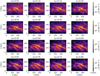 |
Fig. A.1. Maps showing the current density integrated along the z-axis, derived from an ensemble of NLFFF extrapolations with different values for the weighting factor λff. |
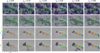 |
Fig. A.2. Comparison of field lines in selected extrapolations from the ensemble. First row: Field lines randomly sampled from the entire bottom boundary. Second row: Same as above, but the low current density regions are transparent. Third row: Field lines corresponding to the area inside the J-shaped flare ribbon. Bottom row: Field lines corresponding to the dimming region as defined by all pixels below the threshold of −0.5 in the logarithmic AIA 211 Åbase ratio image of 20:35 UT (see Sect. 3.2 for more details). In the visualizations of λff = 0.4, two subregions are marked that correspond to the subregions for which the quality metrics given in Table A.1 were calculated. |
Quality metrics for the NLFFF extrapolations using different λff.
All Tables
All Figures
|
Fig. 1. Extent of the bottom boundary of the extrapolation volume (white contours; a rectangle in CEA coordinates) compared with selected full-disk observations before (first and second columns) and during the filament eruption (third column). The pre-eruption SDO/HMI LOS magnetogram and the SDO/AIA 211 Å and 304 Å images, match the time of our NLFFF extrapolation (19:34 UT). The KSO Hα image was recorded at 14:59 UT. |
| In the text | |
|
Fig. 2. Overview of the filament eruption and associated M3.7 flare as observed in selected SDO/AIA channels and GONG Hα filtergrams. The figure is adapted from Purkhart et al. (2025). The movie accompanying this figure shows the full eruption in more wavelength channels. The associated movie is available online. |
| In the text | |
|
Fig. 3. Evolution of the coronal dimming associated with the filament eruption. Upper panel: Time series of STIX counts in three different energy bands. The selected observation times are marked by the red vertical lines. Bottom panels: Selected observation times. Each row corresponds to one time and shows the AIA 211 Å image from that time, the derived LBR map (the base time is 20:00 UT) with instantaneous and cumulative dimming masks (threshold: LBR = −0.5 log10 relative counts), and the HMI LOS magnetogram from 20:00 UT with the same dimming mask contours. The associated movie is available online. |
| In the text | |
|
Fig. 4. Time evolution of the cumulative dimming mask and the extracted parameters of the major dimming region associated with the footprint of the eastern filament leg. Top panel: HMI LOS magnetogram with the dimming mask. The pixels are color-coded according to the time they were first classified as a dimming pixel (threshold: LBR = −0.5 log10 relative counts). Bottom panels: Time evolution of dimming parameters (black). From top to bottom: Cumulative intensity (Icumu), cumulative area (Acumu), cumulative negative flux (Φ−, cumu), and new unsigned magnetic flux density (Bunsigned, new). The time evolution of the derivative of each quantity is shown in blue. The STIX 15-25 keV light curve (green) is included in each panel as a reference. |
| In the text | |
|
Fig. 5. Overview of NLFFF extrapolation results and comparison with observations reprojected to the CEA coordinate frame of the extrapolation. (a) HMI Br magnetogram. The contours show the maximum brightness of flare ribbons in a series of AIA 1600 Å images between 20:00 and 20:45 UT. The contour levels are 25, 100, and 400 DN/s. (b) 5000 field lines randomly started from the lower boundary of the extrapolation volume with the HMI LOS magnetogram and AIA 1600 Å contours as background. The field lines are color-coded according to the local current density. Regions of low current density are made increasingly transparent to keep the underlying high current density filament channel visible. (c) Same as b, but with 50 000 field lines. (d) 5000 field lines with the AIA 211 Å image showing the dimming as a background. The dimming area is marked by a cyan mask. (e and f) reprojected KSO Hα and AIA 211 Å images for reference. The locations of the PIL (green dotted) and inverse J-shaped flare ribbon (white dashed) are indicated on some panels. The movie accompanying this figure shows a smooth transition between the NLFFF extrapolation and the AIA 304 Å and KSO Hα images. The movie is available online. |
| In the text | |
|
Fig. 6. Field lines associated with the core of the MFR (left column), the inverse J-shaped ribbon (middle column), and the coronal dimming region (right column). The field lines start from a single circular seed source at the eastern end of the shown structure (left column); from multiple circular seed sources covering the area inside the inverse J-shaped ribbon, as suggested by the maximum AIA 1600 Å contours (middle column); and from inside the dimming region, as determined by all pixels below the threshold of −0.5 in the logarithmic AIA 211 Å base ratio image of 20:35 UT (see Sect. 3.2 for more details). Each field structure is compared with the HMI Br magnetogram from the NLFFF extrapolation time (top row). Side views from the direction of the colored arrows (red and blue) are shown in the insets. The cyan line roughly indicates the extent of the main part of the flare ribbons. The field structures are compared with the AIA 211, 304 Å, and KSO Hα observations. The dimming mask used as a seed source is shown in the inset of the AIA 211 Å observation. |
| In the text | |
|
Fig. A.1. Maps showing the current density integrated along the z-axis, derived from an ensemble of NLFFF extrapolations with different values for the weighting factor λff. |
| In the text | |
|
Fig. A.2. Comparison of field lines in selected extrapolations from the ensemble. First row: Field lines randomly sampled from the entire bottom boundary. Second row: Same as above, but the low current density regions are transparent. Third row: Field lines corresponding to the area inside the J-shaped flare ribbon. Bottom row: Field lines corresponding to the dimming region as defined by all pixels below the threshold of −0.5 in the logarithmic AIA 211 Åbase ratio image of 20:35 UT (see Sect. 3.2 for more details). In the visualizations of λff = 0.4, two subregions are marked that correspond to the subregions for which the quality metrics given in Table A.1 were calculated. |
| In the text | |
Current usage metrics show cumulative count of Article Views (full-text article views including HTML views, PDF and ePub downloads, according to the available data) and Abstracts Views on Vision4Press platform.
Data correspond to usage on the plateform after 2015. The current usage metrics is available 48-96 hours after online publication and is updated daily on week days.
Initial download of the metrics may take a while.