| Issue |
A&A
Volume 701, September 2025
|
|
|---|---|---|
| Article Number | A227 | |
| Number of page(s) | 11 | |
| Section | Galactic structure, stellar clusters and populations | |
| DOI | https://doi.org/10.1051/0004-6361/202556309 | |
| Published online | 19 September 2025 | |
Asymmetries in the LMC velocity maps
1
Departament de Física Quàntica i Astrofísica (FQA), Universitat de Barcelona (UB),
C Martí i Franquès, 1,
08028
Barcelona,
Spain
2
Institut de Ciències del Cosmos (ICCUB), Universitat de Barcelona,
Martí i Franquès 1,
08028
Barcelona,
Spain
3
Institut d’Estudis Espacials de Catalunya (IEEC),
C Gran Capità, 2-4,
08034
Barcelona,
Spain
4
Lund Observatory, Division of Astrophysics, Department of Physics, Lund University,
Box 43,
22100
Lund,
Sweden
★ Corresponding author: This email address is being protected from spambots. You need JavaScript enabled to view it.
Received:
8
July
2025
Accepted:
31
July
2025
Abstract
Context. The analysis of precise Gaia DR3 astrometry in the LMC region has revealed asymmetric patterns in the bar quadrupole and the disc outskirts of the LMC in-plane velocity maps.
Aims. We aim to quantify the asymmetries detected in the LMC radial and residual tangential velocity maps, and determine whether they are generated naturally due to the LMC’s interaction with the SMC.
Methods. We analyse the velocity maps of different simulations from the KRATOS suite of N-body simulations of the LMC–SMC– MW system, proposing a new methodology to quantify the kinematic asymmetry in the bar and the outskirts of the disc. We also transform the KRATOS simulations into mock catalogues with G magnitudes and Gaia observational errors, to confirm that the asymmetric signature in the LMC is not an effect of observational uncertainties. In addition, we investigate the possibility of a classification bias in the neural network classifier of the Gaia optimal sample.
Results. In the KRATOS simulations of the LMC and SMC interaction, the dynamical effect of the SMC passages produces a displacement of the bar and asymmetries in the LMC velocity maps. Individual stars of the SMC do not have a substantial effect on the kinematics of the LMC. By comparing the velocity maps of mock catalogues of the future Gaia data releases DR4, DR5, and GaiaNIR, we find that the asymmetric signature in the bar quadrupole is independent of observational errors. We thereby confirm that it is a consequence of the interaction of the LMC with the SMC. We also find a classification bias in the neural network classifier, indicating that the outer disc asymmetry observed in the optimal sample is artificial.
Conclusions. The analysis of the KRATOS simulations reveals that the interaction of the LMC with the SMC can generate asymmetric patterns in the velocity field. In the case of the Gaia DR3 LMC velocity maps we conclude that the bar quadrupole asymmetry is directly correlated with the SMC interaction, while the outer disc asymmetry is an artefact of the classifier for the optimal sample.
Key words: Galaxy: kinematics and dynamics / galaxies: interactions / Magellanic Clouds
© The Authors 2025
 Open Access article, published by EDP Sciences, under the terms of the Creative Commons Attribution License (https://creativecommons.org/licenses/by/4.0), which permits unrestricted use, distribution, and reproduction in any medium, provided the original work is properly cited.
This article is published in open access under the Subscribe to Open model. This email address is being protected from spambots. You need JavaScript enabled to view it. to support open access publication.
1 Introduction
The LMC is the largest satellite galaxy of the Milky Way (MW) with a mass of ~1.8 × 10¹¹ M⊙ (e.g. Shipp et al. 2021; Watkins et al. 2024) and at a distance of ~49.59 kpc (Pietrzyn´ski et al. 2019). It is a Magellanic spiral galaxy characterised by a tilted, off-centre bar and a single prominent spiral arm (e.g. Elmegreen & Elmegreen 1980; Zaritsky 2004; Gaia Collaboration 2021; Rathore et al. 2024; Jiménez-Arranz et al. 2025). Recent studies suggest that the LMC’s bar may be non-rotating (Jiménez-Arranz et al. 2024b; Jiménez-Arranz & Roca-Fàbrega 2025). Together, these non-axisymmetric structures are likely the result of the interactions of the LMC with the SMC, one of its satellite galaxies located at a distance of around 62 kpc from the MW (Cioni et al. 2000; Hilditch et al. 2005; Graczyk et al. 2013). The LMC and SMC (hereafter MCs) are separated 20–25 kpc and, among others, a prominent feature of their interaction is the trail of stars that lies between both of them. This structure, called the Bridge, consists mostly of SMC gas and stars that have been stripped from the SMC during past tidal interactions with the LMC, (e.g. Misawa et al. 2009; Skowron et al. 2014; Carrera et al. 2017; Zivick et al. 2019; Gaia Collaboration 2021). Due to their proximity to us, individual stars of the MCs can be resolved (e.g. Nidever et al. 2017; Gaia Collaboration 2021; Niederhofer et al. 2022; Jiménez-Arranz et al. 2023b,a). This makes the MCs a unique opportunity to study the effects of the interaction between galaxies on their internal structures and their evolution history.
ESA’s Gaia mission is providing astrometric, photometric, and spectroscopic data for more than 1.8 billion stars, of which about 10-20 million correspond to the MCs (Jiménez-Arranz et al. 2023b, hereafter JA23; Jiménez-Arranz et al. 2023a). From these measurements, we can derive 3D kinematic maps of the LMC that reveal rich complexities and substructures in the LMC disc (Gaia Collaboration 2021; Choi et al. 2022; Cullinane et al. 2022; JA23; Jiménez-Arranz et al. 2025; Vijayasree et al. 2025). One of these features is a largely asymmetric kinematic signature in the bar region (see Fig. 1). If the bar were located in the centre of mass of an unperturbed system, we would expect a perfectly symmetric quadrupole, with a positive–negative trend in each pole due to the elliptic shape of the stellar orbits in the bar. The kinematic maps also show strong inward and outward velocities in the outer regions of the LMC disc, particularly strong inward velocities (blue) in the upper region of the radial velocity map (left panel of Fig. 1), which are not mirrored in the symmetric region in the lower part of the map. The unknown origin of the bar and disc asymmetries in the Gaia data motivates a pursuit to correlate asymmetric kinematic maps with irregular bars and galaxies in interaction.
Numerical simulations have been developed to model the past orbit of the LMC, investigate the dynamical effects of its interaction with other galaxies, and explore the time evolution that cannot be captured by observational data alone (Besla et al. 2012; Garavito-Camargo et al. 2019; Lucchini et al. 2021; Vasiliev 2023; Sheng et al. 2024; Sheng et al. 2025; Brooks et al. 2025). In this work, we use the KRATOS simulations (Jiménez-Arranz et al. 2024b, hereafter JA24), a large suite of N -body simulations designed with a high spatial, mass, and temporal resolution, aiming to study the internal kinematics of the LMC and its interactions with the SMC and the MW. This study aims to analyse the kinematic maps of LMC-like galaxy simulations to study how the interaction with an SMC-mass simulation can cause the asymmetries in the inner bar region as well as the outer regions of the LMC disc. We investigate whether the asymmetries observed in JA23 using Gaia DR3 data can be reproduced in N -body simulations and therefore be a natural consequence of the LMC’s evolution, particularly considering its interaction with the SMC. We also use these simulations to generate velocity maps, applying the expected uncertainities of future Gaia and GaiaNIR releases to evaluate the effect of present Gaia uncertainties.
The article is organised as follows: in Sect. 2 we describe our datasets. Sect. 3 details the methods used to quantify the asymmetries in our analysis. An overview of the results is given in Sect. 4. We add a discussion on observational uncertainties and possible sample bias in Sect. 5, as well as a further exploration of the KRATOS simulations and future Gaia and GaiaNIR data in Sect. 6. We summarise our work and present our conclusions in Sect. 7.
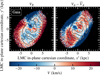 |
Fig. 1 Comparison of the radial VR (left panel) and residual tangential |

2 Data and kinematic maps
2.1 LMC Gaia DR3 clean samples
Gaia DR3 (Gaia Collaboration 2023) gives us access to detailed astrometric information for a catalogue of more than 1.8 billion stars, of which about 10-20 million belong to the MCs (JA23; Jiménez-Arranz et al. 2023a). In this work, we use the LMC optimal sample from JA23. This dataset was selected using a neural network classifier and contains 9 810 031 candidate LMC stars. Using the coordinate transformation introduced by van der Marel (2001), van der Marel et al. (2002) and used in JA23, with inclination angle i = 34°, and position angle θ = 220° (Gaia Collaboration 2021), we deproject the LMC to obtain the LMC in-plane (x′, y′) Cartesian co-ordinates. The top panel of Fig. 2 shows the density map of the LMC optimal sample, face-on in the LMC in-plane (x′, y′) Cartesian coordinate system.
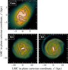 |
Fig. 2 Density maps of the LMC optimal sample using Gaia DR3 data (top panel, JA23) and GLMC disc of the K4 and K6 simulations from the KRATOS suite (bottom panels, JA24). All maps are shown face-on, in the LMC in-plane (x′,y′) Cartesian coordinate system. Black contour lines separate the overdensities (bar and spiral arms) from the underdensities. The KRATOS simulations are shown at t = 0.105 Ga (see Sect. 4.3 for discussion). |
2.2 KRATOS simulations
We aim to compare the Gaia DR3 LMC optimal sample with the KRATOS simulations (JA24), a suite of N-body simulations of isolated and interacting LMC-like galaxies. KRATOS consists of 28 simulations that model the evolution of an LMC-like galaxy with varying parameters. The suite includes models in which the LMC-like galaxy is in isolation or in interaction with an SMC-mass galaxy and a MW-mass galaxy. In this work we follow the notation introduced in JA24, where the LMC-like galaxy is denoted as GLMC, and the SMC- and MW-mass systems as GSMC and GMW, respectively. In the suite of simulations, the parameters explored are the mass of the baryonic matter or dark matter content of the GLMC, the stellar Toomre parameter Q of the GLMC, and the mass of the GSMC or the GMW, if present (see Table 2 of JA24 for a summary). All simulations were evolved for 4.68 Ga with a spatial and temporal resolution of 10 pc and 5000 yr, respectively, and a minimum mass per particle of 4 × 10³ M⊙. Details and specific characteristics of each of the 28 simulations can be found in Sect. 2 of JA24.
The simulations analysed in this work are K4 and K6, shown in the bottom panels of Fig. 2. The K4 simulation models an isolated GLMC system, whereas the K6 simulation matches its GLMC parameters but includes the full interacting system of GLMC, GSMC, and GMW. This set of simulations was chosen for this work due to the K6 simulation’s morphological similarities with the LMC, in particular its off-centre bar (bottom right panel, Fig. 2). The time stamps are defined with respect to the t = 0 Ga established in JA24 (see Sect. 4.3 for further discussion).
To compare the internal kinematics of the KRATOS simulations to those of the deprojected Gaia DR3 LMC optimal sample, we determine the KRATOS simulations’ GLMC in-plane position and velocity co-ordinates, (x′, y′, v′x, v′y). We first centre the reference frame in the centre of mass of the GLMC baryonic matter. Then we correct for the GLMC systemic motion and align the reference frame so that the (x′,y′)-plane coincides with the GLMC disc plane by computing the disc angular momentum (see Sect. 2.3 of JA24 for details).
2.3 Kinematic maps
From the LMC and GLMC in-plane position and velocity coordinates we created galactocentric radial VR and residual tangential  velocity maps. The radial velocity maps show the stars’ motion towards (negative) or away from (positive) the galactic centre, while the residual tangential velocity maps show if the stars are moving faster (positive) or slower (negative) than the galaxy’s mean tangential velocity curve at their radial distance from the galactic centre. Figure 3 presents the radial (left) and residual tangential (right) velocity maps for the LMC optimal sample (top panels) and the KRATOS simulations (centre and bottom panels). The binned kinematic maps were obtained by dividing the sample of stars in a square grid with 0.16 × 0.16 kpc bins. Due to the different spatial extent of the Gaia data compared to the simulation, we used 125 × 125 bins to display −10 to 10 kpc in both x′ and y′ for the LMC optimal sample (top panels), and 200 × 200 bins for the simulated KRATOS discs from −16 to 16 kpc (centre and bottom panels). For each bin, we computed the median of the radial or residual tangential velocities of the enclosed stars. Contour lines (in black) based on the respective source overdensity map of the LMC (see Fig. 2), trace the bar and spiral arm(s) on the velocity maps.
There are two notable features in these kinematics maps. First, a barred galaxy presents a characteristic quadrupole pattern in the radial velocity VR and residual tangential velocity  maps. This signature stems from the elliptical orbits of the stars that make up the bar as seen from the centre of the bar. This quadrupole is seen in the blue (red), negative (positive) velocities of the bins inside and near the bar contours. The quadrupole of the K4 simulation is symmetric (middle row of Fig. 3) because no perturbation is present and the centre of mass and centre of the bar coincide. On the other hand, for the LMC optimal sample and the K6 simulation (top and bottom rows of Fig. 3), the centre of mass and centre of bar do not coincide (see also Fig. 9 of JA24 for the off-centredness evolution of the GLMC bar), making the quadrupole signal in the radial velocity and residual tangential velocity maps asymmetric.
Second, the outer region of the LMC disc presents a high inward velocity in the upper region of the Gaia radial velocity map (top left panel of Fig. 3), which is unmatched on the opposite side of the galaxy. A similar feature of opposite sign can be seen in the high outward radial velocity in the lower right region of the GLMC disc outskirts of the K6 simulation (bottom left panel of Fig. 3).
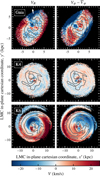 |
Fig. 3 Comparison of the radial VR (left panels) and residual tangential |

3 Quantitative analysis of the asymmetries
In this section, we devised two methods to analyse the asymmetries in the LMC bar and disc outskirts. We used the kinematic maps described in Sect. 2.3 to apply the methods first to the KRATOS simulations (Sects. 3.1 and 3.2) and then to the LMC Gaia data (Sect. 3.3).
3.1 GLMC bar
In order to analyse the bar region of the KRATOS simulations, we binned the stars in a zoomed-in square grid, using 200 × 200 bins for −4 to 4 kpc, which yields bin dimensions of 0.04 × 0.04 kpc. We selected the bar region of the velocity maps using a contour, marking where the local density is at least 20% higher than the Gaussian smoothed background. To quantify the asymmetry of the bar, we then computed the median radial, VR, and residual tangential,  , velocity of stars that were binned inside this bar contour.
For an unperturbed bar with a symmetric quadrupole, the median bar velocity would be zero because the velocities of opposite quadrants cancel out. A deviation from zero therefore indicates an asymmetry in the bar quadrupole. For the KRATOS simulations, we can analyse the time evolution of the bar quadrupole using consecutive snapshots (see Sect. 4.1).
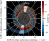 |
Fig. 4 Visualisation of the outer disc quantitative analysis. We show the radial velocity map of a GLMC disc of the KRATOS suite, with the disc divided into 20 angular wedges of 18° each. The first pair of opposite wedges is highlighted while the others are masked by higher opacity. The centre of the disc is further masked by a circle of radius R = 6 kpc. |
3.2 GLMC outer disc
We analysed the asymmetries in the outer regions of the GLMC disc of the KRATOS simulations in the steps listed below and illustrated in Fig. 4:
We masked the inner region of the GLMC disc with a circle of radius R = 6 kpc.
We split the disc into 20 angular wedges of 18° each. Then we computed the median value of VR and
 in each section.
As a measure of the azimuthal symmetry of the regions of the GLMC disc, we subtracted the median velocity of each wedge by its opposite wedge’s median velocity (for example, the pair of wedges highlighted in Fig. 4).
If the resulting subtracted median velocity deviates greatly from the expected value of zero, it indicates an asymmetry in the GLMC disc. To obtain a quantification of the maximum or minimum asymmetry of the disc per snapshot, we computed the extrema of the subtracted median velocities across the whole disc, EXT 〈VR〉 and EXT
 .
.
We repeated this process for successive snapshots to analyse the time evolution of the asymmetries in Sect. 4.2.
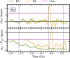 |
Fig. 5 Mean radial velocity, 〈VR〉 (top panel), and mean residual tangential velocity, |

3.3 LMC Gaia data
To quantify the bar asymmetries in the LMC optimal sample from Gaia data, we fit an ellipse with an axis ratio of q = 0.46, an angle of φ = 154.18° (both from Choi et al. 2018), and a semi-major axis of 2.3 kpc (Jiménez-Arranz et al. 2024a). Then, similarly to the GLMC bar analysis (see Sect. 3.1) we computed the median radial, VR, and residual tangential,  , velocities of the bins enclosed in this ellipse. To analyse the asymmetries in the outer regions of the LMC optimal sample, we followed the same steps as outlined in Sect. 3.2, but masking the inner 4kpc of the disc, instead of the inner 6 kpc. This analysis provides two extrema for the Gaia outer disc, one for the median radial velocity, EXT 〈VR〉, and one for the median residual tangential velocity, EXT
  . Since we do not have any time evolution in the Gaia data, we recover single values for the median velocities of the LMC bar, and for the extrema of the outer disc median velocities.
4 Results
4.1 Asymmetry in bar kinematics
To analyse how the asymmetry of the GLMC bar changes with time, we show the evolution of the K4 and K6 simulations’ median radial, 〈VR〉, and residual tangential,  , velocity of the bar in Fig. 5. The quadrupole of the K4 simulated bar is symmetric with only small deviations from zero in 〈VR〉 (top panel, green line) after bar formation at approximately t–2 Ga. Similarly, the
  (bottom panel, green line) does not show abrupt variations, but gradually becomes more negative. This is because the bar lengthens over time (see for example Fig. 8 of JA24), causing the bar contour to capture more of the negative residual tangential component.
In the interacting K6 simulation, both 〈VR〉 and  (top and bottom panel, yellow line) vary significantly after bar formation at approximately t = −1.34 Ga. The bar formation of the K6 simulation occurs later than that of K4, namely after the first pericentric passage of the GLMC–GSMC. After this interaction, both the median radial and median residual tangential velocity deviate from zero. Particularly after the second pericentric passage between the GLMC–GSMC at t ∼ −0.15 Ga, there is a maximum in the median radial velocity of the bar, immediately followed by a maximum in the median residual tangential velocity. For comparison, we mark the asymmetry of the Gaia data with horizontal, purple lines in both panels. For both the radial and the residual tangential velocity, the Gaia bar asymmetry line passes through the peaks of the K6 simulation asymmetry, shortly after the second pericentric passage.
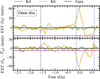 |
Fig. 6 Same as Fig. 5 but for the outer disc asymmetry evolution of the GLMC, represented by the extrema in the disc velocities for each snapshot from the K4 (green lines) and K6 (yellow lines) simulations. |
4.2 Asymmetry in outer disc kinematics
To analyse the changes in the kinematics of the GLMC outer disc, we apply the method described in Sect. 3.2 to the full temporal evolution of the K4 and K6 simulations. Computing the extrema in the kinematic map velocities for different timestamps provides us with the evolution of the disc outskirts’ asymmetry over time, shown in Fig. 6. Similarly to the time evolution of the bar in Sect. 4.1, the unperturbed K4 simulation shows no significant variation in the extrema of 〈VR〉 or  (top and bottom panels, green lines), indicating symmetry in the disc outskirts. In contrast, the interacting K6 simulation has a maximum in the extrema of the mean radial velocities (upper panel, yellow line) after the second pericentric passage of the GSMC at t ∼ −0.15 Ga. At this time, the GLMC disc outskirts have a large asymmetric feature of positive radial velocity, which is unmatched on the opposite side of the disc. The same time stamp is also characterised by a minimum in the mean residual velocities (bottom panel, yellow line), which signifies a strong asymmetry skewing to negative residual tangential velocity of the disc. Another local extremum of lower amplitude can be seen after the first pericentric passage of the GSMC around t ∼ −1.58 Ga, in both the radial and residual tangential velocities. Again, we also show the asymmetry of the Gaia data by marking horizontal purple lines for the extrema of the median radial and median residual tangential velocities of the disc outskirts. Here we see that the Gaia asymmetry line passes through the minimum of the K6 radial velocity extrema, but it is close to zero in the residual tangential velocity extrema.
4.3 Re-evaluating t = 0
The initial conditions and orbital parameters of GLMC, GSMC, and GMW in KRATOS were based on the work by Lucchini et al. (2021) and the “present time” t = 0 Ga was determined to match the number of GLMC–GSMC pericentric passages and the morphology of the GLMC disc, rather than the GLMC closest approach to the GMW (see Sect. 3 of JA24 for more details). While the “present time” considered in KRATOS qualitatively matches the morphology of the present-day LMC disc, in this work we aim to redefine the timestamp t = 0 Ga in the KRATOS simulation to match more closely with the kinematic maps of the Gaia DR3 LMC optimal sample.
Due to the complexity of the asymmetric features on a perturbed disc, we cannot simply define the new t = 0 based on the intersection of the Gaia asymmetry line (purple line) with the asymmetry evolution plots of the K6 simulation in Figs. 5 and 6. Around these intersection points in the K6 simulation, we mainly find snapshots where the bar has been completely destroyed, or the disc outskirts have bimodal velocities due to the recent passage of the GSMC. To best match the complex asymmetries of the kinematic maps, we instead select a broad range of timestamps around the second pericentric passage and visually inspect the kinematic maps.
We find a closer representation of the LMC optimal sample asymmetry at t = 0.105 Ga, shown in the bottom row of Fig. 3. Both the LMC optimal sample (top row) and the K6 simulation (bottom row) have an off-centre bar and one broken spiral arm. The velocity maps show similar trends but with opposite signs: in the LMC optimal sample, the bar’s quadrupole has strong asymmetry in the negative radial velocity, whereas the K6 snapshot has a similar asymmetric feature in the positive radial velocity. There are similar patterns of negative residual tangential velocity in both bars, including some asymmetry. In the disc outskirts, we see negative radial velocities in the top left of both maps, whereas the rest of the outskirts are dominated by positive radial velocities. We are unable to match the outskirts in the residual tangential velocity with the strong negative velocities along opposite sides of the disc. However, this feature is likely a result of the galaxy’s morphology, because we compute the residual tangential velocity by subtracting radially binned mean tangential velocities, despite the LMC’s elongated disc. For future studies using the KRATOS simulations, we recommend that the snapshot at time t = 0.105 Ga1 from the K6 simulation be used as the “present time”, because it not only represents the morphology of the LMC but also resembles its velocity maps more closely.
5 Cause of asymmetries
In this section, we explore several possible causes of the asymmetries seen in the kinematic maps of the Gaia LMC optimal sample (JA23) and characterised in this work. First, in Sect. 5.1, we present our study of LMC–SMC interactions using the KRATOS suite (JA24) to explain the asymmetries described in Sect. 4. Then we discuss the possibility of a bias in the LMC optimal sample stemming from the neural network classifier in Sect. 5.2, and address the potential effect of the observational errors of Gaia in Sect. 5.3. Lastly, we repeat the asymmetry analysis for a larger sample of KRATOS simulations in Sect. 5.4 to verify the consistency of our results.
5.1 LMC-SMC interaction
From the K4 simulation in Figs. 5 and 6 (green lines) we can see that an isolated GLMC does not generate a significant asymmetry in the bar, or in the outer disc. Without an external perturbation such as the GLMC – GSMC interaction, the median radial and median residual tangential velocities of the GLMC do not show significant variation over time. In the K6 simulation, on the other hand, there are extrema in the velocity maps of both the bar and the outer disc (yellow lines). We can furthermore see that the extrema are correlated in time with the pericentric passage of the GSMC. Therefore, we can conclude from the KRATOS simulations that the asymmetries observed in the LMC disc of Gaia data may arise naturally due to the interaction of the LMC with the SMC.
Additionally, since the inward motion in the radial velocity map of the LMC optimal sample is located in the direction of the Bridge, the authors in JA23 hypothesised that it could be a signature of SMC stars accreting into the LMC. Using the K6 simulation, we evaluate whether the GSMC stars in the GLMC kinematic maps could gnerate the asymmetries seen in Gaia data, by presenting velocity maps that include the stellar particles of the GSMC. We show in Fig. 7 that, while the GSMC stars are crossing the disc of the GLMC, their presence alone does not change the kinematic maps significantly. Instead, the GSMC’s pericentric passage induces an overall dynamical effect on the kinematic maps of the GLMC. However, the sign and amplitude of the changes in the velocity maps depend on the orbit of the GSMC around the GLMC, and in the KRATOS simulations we do not have the true orbits to qualitatively reproduce the exact signature we observe in the Gaia data.
5.2 Bias in the LMC optimal sample classifier
A classification bias in the neural network classifier of the LMC sample from JA23 could affect the generated velocity maps, because a misclassification of LMC stars in some regions could result in a distribution of velocities that is biased with respect to the distribution of the true LMC population. To investigate this possible bias, we compared the density and radial velocity maps of different LMC samples obtained from the neural network classifier in Fig. 8. We show the complete sample (top row), as defined by JA23 with a probability cut of Pcut = 0.01, and the optimal sample (middle row), with a cut of Pcut = 0.52, where stars with P > Pcut are considered part of the LMC. The bottom row shows the difference between the two samples.
The radial velocity maps (right column) show that the asymmetry in the disc outskirts becomes much more pronounced in the optimal sample (middle row), which is a clear indication of a possible bias, since there is no physical reason for this change between the two samples. To highlight this, in the bottom right panel we show the difference between the complete and optimal sample’s velocity maps, which has large structures of positive radial velocity in the upper left corner and negative radial velocities along the sides. These features are most likely artefacts of the classifier and would not be present in an unbiased sample. Even though the LMC–SMC interaction can explain asymmetries in the disc outskirts (see Sect. 5.1), we can therefore conclude that the asymmetry in the disc outskirts of the Gaia optimal sample radial velocity map is a consequence of the sample selection.
The misclassification can likely be attributed to limitations of the neural network’s training sample. As shown in Figure 2 of JA23, The proper motion distribution of the base Gaia sample in right ascension and declination is broader than that of the training set, which is centred on the systemic motion of the LMC. As a result, the classifier performs best for stars near the centre of the LMC, while objects in the outskirts are more likely to be misclassified due to the difference in proper motion from the centre to the outskirts of the LMC. Since a purer sample more closely resembles the training sample, it also inherits its limitations. We therefore recommend the use of the complete sample in future studies of the outer disc.
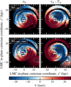 |
Fig. 7 Comparison of the radial, VR (left panels), and residual tangential, |

5.3 Gaia observational errors and selection function
To verify that the asymmetries in the velocity maps are not a result of observational uncertainties, we applied Gaia DR3 observational errors to the KRATOS simulations. To this end, we projected the GLMC to the position and orientation of the LMC in the heliocentric reference frame, using centre coordinates (α0,δ0) = (81.28°, −69.78°) (van der Marel 2001), inclination angle i = 34°, and position angle θ = 220° (Gaia Collaboration 2021). The effect of a different inclination or position angle on the kinematic maps has been studied in Jiménez-Arranz et al. (2023b), where no resulting systematic asymmetry was observed. From the projected KRATOS simulations, we created a mock catalogue of Gaia observable parameters2: positions (α, δ), parallax (ϖ), and proper motions (μα,μδ).
We used a 3D extinction model (Marshall et al. 2006; Lallement et al. 2022), which is also applied in the Gaia Object Generator (GOG, Luri et al. 2014). To assign Gaia photometry to the simulated particles, we assumed red clump (RC) stellar parameters, since RC stars are dominant in the LMC (Gaia Collaboration 2021). From the absolute magnitude Mk = −1.61 and intrinsic colour (J - K)0 = 0.55 of RC stars (Ruiz-Dern et al. 2018; Straižys & Lazauskaitė 2009), we computed G magnitudes for each particle. Then we used the Gaia DR3 error model of PyGaia (Brown et al. 2012) to assign uncertainties in position (σα*, σδ), parallax (σw), and proper motion (σμα, σμδ)3.
In order to evaluate the completeness of Gaia in the LMC region, we applied the Gaia selection function from Castro-Ginard et al. (2023), which estimates the probability that an input source is included in Gaia DR3. Using GaiaUnlimited4 (Cantat-Gaudin et al. 2023; Castro-Ginard et al. 2023), we created a sub-selection function, binning by colour GBP - GRP and magnitude G of RC stars. We show the result of this selection function per healpix region in Fig. 9. In the LMC disc, Gaia has a high completeness with a selection probability of close to 1.0, even in the crowded bar region. However, since we are limiting this sub-selection function to RC stellar parameters, the outskirts and surroundings of the LMC are undersampled. Therefore, the sub-selection function cannot be directly applied to the KRATOS simulations, which do not match the LMC’s morphology and spatial extent. Instead, we applied the general Gaia survey selection function to the mock catalogue. This function is homogeneous in the LMC region with high completion everywhere except in the crowded bar.
We then converted our Gaia mock catalogue back to the LMC in-plane coordinate frame, shown in Fig. 10. We compare the original K6 simulation (top row) with the mock catalogue (middle row), and their residuals (bottom row). We find that the effect of crowding in the bar region of the LMC removes less than 1% of the stars in our sample, and the asymmetric signature in the bar is still visible (middle row of Fig. 10). The observational uncertainties and selection function of Gaia data are therefore not sufficient to explain the asymmetric signal in the bar region. In the disc outskirts, the general Gaia selection function has high completeness, but the astrometric uncertainties have a larger impact.
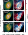 |
Fig. 8 Comparison of the density maps (left panels) and radial velocity maps (right panels) according to the neural network classification in JA23 of the complete sample (top row), optimal sample (middle row), and the difference between complete and optimal sample (bottom row). All maps are seen face-on, in the LMC in-plane (x' ,y') Cartesian coordinate system. A black contour line separates the LMC overdensities (bar and spiral arms) from the underdensities. |
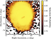 |
Fig. 9 Sub-selection function from GaiaUnlimited for RC stellar parameters (GBP - GRP colour from −0.1 to 0.4 and magnitude G = 18-20 mag), for the LMC region with centre co-ordinates (α0, δ0) = (81.28°, −69.78°) (van der Marel 2001). |
5.4 Consistency of results among the KRATOS suite
In order to test the ubiquity of asymmetry in interacting simulations, we analyse the additional interacting models of the KRATOS suite. In Fig. 11, we show our analysis of the asymmetry evolution in the bar (left two columns) and in the disc outskirts (right two columns) and note the following features:
K3, K6, and K9 (first row) have the same masses and therefore the same orbits and pericentric passages. Differences between the models affect only the internal structure of the GLMC due to their different stellar Toomre parameter Q. Consequently, there are minimal differences in the outer disc asymmetry among the models, but K6 (yellow line) shows some variation even before the first pericentric passage, since it has the lowest Toomre parameter, Q = 1.0. All models show large variation correlated with the pericentric passages, particularly the second. The same is true for the bar asymmetry evolution, where all models form bars only after the first pericentric passage, and have larger variation after the second and third.
K12 (second row) and K21 (fifth row) have lower GLMC dark matter halo masses, and therefore have only one late pericentric passage. Additionally, these pericentric passages happen at larger distances of about 13–14 kpc from the GLMC, compared to the fiducial (K3) pericentric passages at distances of about 12 and 5 kpc. This leads to very small asymmetries in the outer disc for both K12 and K21. Of the two, K21 (lime green) has larger variation in bar asymmetry after the pericentric passage because the model also has a lower GLMC disc mass.
K15 and K24 (third row) have the same GLMC dark matter halo, which has a higher mass than the fiducial and therefore causes their identical pericentric passages to happen earlier than in the fiducial simulations. Even though the K15 and K24 have different GLMC disc masses, their outer disc asymmetry evolves very similarly. K15 forms a bar despite the large mass of its dark matter halo, and then has some bar asymmetry after the second pericentric passage. K24 does not form a bar due to its lower disc mass.
K18 (fourth row) has very similar pericentric passages to K3, K6, and K9, because its only difference from the fiducial is a smaller GLMC disc mass. The bar is formed later than in the fiducial model, but the asymmetry variations are similarly more prominent after the second and third pericentric passages.
K26 (sixth row) has a reduced GSMC mass and therefore only one pericentric passage, which happens at a large distance of around 17 kpc and therefore causes the least variation in the outer disc asymmetry evolution. In this model, the GLMC never forms a bar.
K27 (seventh row) has a lower GMW mass and therefore has the closest GLMC –GSMC pericentric passages, at distances around 6.5 and 1 kpc, causing high asymmetry already after the first pericentric passage. The second pericentric passage destroys the bar shortly after its formation, but it is reformed before the third pericentric passage.
K28 (last row) has the same masses as K3, K6, and K9, but a point-like GMW. This changes the orbits so that the pericentres are at larger distances, around 13 and 12 kpc. As a result, the asymmetries have lower amplitudes compared to K3, K6, and K9.
Across all simulations, there are two consistent trends: asymmetries in the velocity maps are correlated in time with pericentric passages, and closer pericentric passages cause larger variations in the asymmetry.
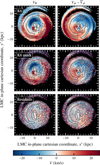 |
Fig. 10 Comparison of the radial VR (left panels) and residual tangential |

6 Improvement of LMC internal kinematics
In this section, we discuss how the asymmetry signal changes with improvements in the observational data. We applied the tool presented in Sect. 5.3 to the K6 simulation to obtain mock catalogues representative of Gaia DR4 and DR5 (Sect. 6.1), and the proposed GaiaNIR (Sect. 6.2).
6.1 Gaia DR4 and DR5
Using the mock catalogues, we can make further predictions of the ability of future Gaia data releases to capture the signatures of asymmetry in the LMC disc. We used the parallax uncertainty relation and applied the scaling factors listed in Table 1 from PyGaia (Brown et al. 2012) to compute the uncertainties in positions and proper motions of future Gaia data releases.
Although the uncertainties of Gaia DR4 and DR5 will be significantly reduced, the velocity maps of the mock catalogues do not show large differences (top rows of Fig. 12). In particular, the bar signature in the centre remains virtually unchanged, although sharper than in DR3 (Fig. 10). We can conclude that the asymmetric features in the velocity maps are not simply a result of the large uncertainties in the Gaia DR3 data, because lower uncertainties reveal the same asymmetries. However, we expect to resolve more details about the disc outskirts in future Gaia data releases.
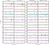 |
Fig. 11 Bar asymmetry evolution (left two columns) and outer disc asymmetry evolution (right two columns), shown with cubic spline fits for all KRATOS simulations that include the full GMW–GLMC–GSMC interaction. Models are grouped together if they share pericentric passages between GLMC–GSMC (vertical dashed blue lines) at the same timestamps. The bar asymmetry evolution is measured in mean radial velocity, 〈VR〉 (left-most panels), and mean residual tangential velocity, |


6.2 GaiaNIR
While Gaia observations are limited to the visible spectra, a planned follow-up astrometric mission will extend the wavelength range into the near-infrared (NIR, Hobbs et al. 2021; Hobbs et al. in prep.). The GaiaNIR mission is aimed at exploring dust-obscured regions of the MW, including the bulge, spiral arms, and other star-forming regions. The all-sky observations will naturally include a large sample of LMC stars, particularly dimmer stars due to the depth of anticipated GaiaNIR observations. Using the predicted uncertainties of the GaiaNIR mission from Hobbs et al. (in prep.), we can evaluate the applications of GaiaNIR data to our science goals and discuss the resulting advances in the study of LMC kinematics.
We computed GaiaNIR uncertainties for two proposed mission sizes, medium and large, each for a 10-year mission duration. We ran the uncertainty computation by Hobbs et al. (in prep.) with a K5III stellar spectrum to simulate RC stars. In Fig. 13 we show the uncertainties in the proper motions of the mock catalogues derived in Sect. 5.3. The uncertainties decrease significantly from Gaia DR4 and DR5 to the GaiaNIR missions, with an additional improvement from the medium (M10, yellow) to the large GaiaNIR mission (L10, orange). The velocities in our LMC radial and residual tangential velocity maps are derived from the proper motions, and the mock catalogues and residuals of the VR maps of the GaiaNIR M10 and L10 missions are shown in the bottom rows of Fig. 12. Since we evaluate a velocity range from −25 to 25 km/s, and the changes between the missions are on the order of 2 km/s, we do not see visible differences in the binned velocity maps.
Furthermore, in applying predictions of GaiaNIR uncertainties to the mock catalogue, we are faced with the limitation of using only RC stars as the stellar tracer of the LMC. For RC stars, the GaiaNIR uncertainties do not significantly improve the velocity maps with respect to Gaia DR5, because RC magnitudes are brighter than the expected GaiaNIR magnitude limit. We will therefore evaluate GaiaNIR uncertainties in the mock catalogue using, for example, main-sequence turnoff stars as tracers in future work.
Gaia uncertainty scaling factors for the different Gaia data releases (Brown et al. 2012).
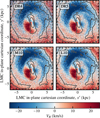 |
Fig. 12 Comparison of the radial velocity maps of mock catalogues from the K6 simulation with observational errors of Gaia (DR4 and DR5, top row) and GaiaNIR (M10 and L10, bottom row). All maps are shown in the LMC in-plane (x′, y′) Cartesian coordinate system and zoomed-in to the centre co-ordinates to show the bar signature. Black contour lines separate the overdensities (bar and spiral arms) from the underdensities. |
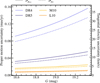 |
Fig. 13 Proper motion uncertainty and tangential velocity uncertainty as a function of G magnitude, for mock catalogues applying errors of different releases of Gaia (DR4 and DR5) and GaiaNIR (M10 and L10). We show the uncertainties in proper motion in right ascension σµα∗ (solid lines) and in declination σµδ (dashed lines). |
7 Conclusions
In this work, we have presented a method to quantify the LMC kinematic asymmetries in the bar region and the outer disc previously noted by JA23. We analysed the KRATOS suite of N -body simulations (JA24) of LMC-like galaxies in isolation or in interaction with SMC- and MW-mass systems and found that the dynamical effect of the SMC can naturally cause asymmetries in the LMC kinematics. We also connected our analysis of the KRATOS simulations to Gaia observations of the LMC using the LMC optimal sample (JA23). We explored possible causes of the asymmetries, including a bias in the LMC optimal sample classifier, and used our mock catalogue tool to evaluate the effects of the uncertainties from Gaia observational errors and the selection function. Lastly, we also considered the improvements of LMC kinematics studies with future releases of Gaia and GaiaNIR data. The main findings of this work are the following:
We have identified a velocity map of the K6 simulation at t = 0.105 Ga that better matches the features of the LMC optimal sample velocity maps (bottom row of Fig. 3). We recommend its use as the “present time” in future work with KRATOS.
As expected, an isolated GLMC does not present the same asymmetries found in cases where the GSMC is included (Figs. 5 and 6).
The velocity maps do not change when GSMC stars are incorporated, suggesting that the effect of the GSMC on the GLMC is purely dynamical (Fig. 7).
We investigated the observational uncertainties in Gaia data as a potential cause of kinematic asymmetries and found a bias in the LMC optimal sample classifier (Fig. 8). We therefore conclude that the asymmetry in the outskirts of the disc observed in this sample is not intrinsic to the LMC but stems from this bias.
In KRATOS, asymmetries in the velocity maps of the bar and outer disc are generally correlated with pericentric passages, and closer pericentric passages cause larger variations in the asymmetry (Fig. 11).
Although we lack time evolution in the Gaia data, we can use our method to quantify the current asymmetry in the LMC optimal sample (Figs. 5, 6, and 11).
From our study of mock catalogues we found that applying Gaia observational errors to the simulations does not significantly change the asymmetric signal in the bar quadrupole of the velocity maps (Fig. 10). We conclude that this asymmetry in the LMC is due to its interaction with the SMC.
The quadrupole signature is preserved independently of observational uncertainties, including the mock catalogues of future data releases Gaia DR4, Gaia DR5, and GaiaNIR (Fig. 12).
We therefore conclude that the asymmetries in the LMC bar of the Gaia velocity maps are a result of the interaction history between the LMC and the SMC, while the outer asymmetry observed in the LMC optimal sample is an effect of the sample classifier.
Acknowledgements
We thank the anonymous referee for providing constructive comments that improved the quality of this paper. We thank A. Castro-Ginard for insightful discussions and help in creating the Gaia selection function using GaiaUnlimited. This work has made use of data from the European Space Agency (ESA) mission Gaia (https://www.cosmos.esa.int/gaia), processed by the Gaia Data Processing and Analysis Consortium (DPAC, https://www.cosmos.esa.int/web/gaia/dpac/consortium). Funding for the DPAC has been provided by national institutions, in particular the institutions participating in the Gaia Multilateral Agreement. M.S. acknowledges funding by the European Union under the Horizon Europe Marie Skłodowska-Curie Actions Doctoral Network grant agreement no. 101072454 @HorizonEU research and innovation programme. O.J.A. acknowledges funding from “Swedish National Space Agency 2023-00154 David Hobbs The GaiaNIR Mission” and “Swedish National Space Agency 2023-00137 David Hobbs The Extended Gaia Mission”. M.R.G. and X.L. acknowledge that this work was (partially) supported by the Spanish MICIN/AEI/10.13039/501100011033 and by “ERDF A way of making Europe” by the European Union through grant PID2021-122842OB-C21, and the Institute of Cosmos Sciences University of Barcelona (ICCUB, Unidad de Excelencia María de Maeztu) through grant CEX2019-000918-M.
References
- Belokurov, V., Erkal, D., Deason, A. J., et al. 2017, MNRAS, 466, 4711 [Google Scholar]
- Besla, G., Kallivayalil, N., Hernquist, L., et al. 2012, MNRAS, 421, 2109 [Google Scholar]
- Brooks, R. A. N., Sanders, J. L., Dillamore, A. M., Garavito-Camargo, N., & Price-Whelan, A. M. 2025, arXiv e-prints [arXiv:2507.10667] [Google Scholar]
- Brown, A. G. A., Leiden University, & Gaia DPAC. 2012, PyGaia [Google Scholar]
- Cantat-Gaudin, T., Fouesneau, M., Rix, H.-W., et al. 2023, A&A, 669, A55 [NASA ADS] [CrossRef] [EDP Sciences] [Google Scholar]
- Carrera, R., Conn, B. C., Noël, N. E. D., Read, J. I., & López Sánchez, Á. R. 2017, MNRAS, 471, 4571 [Google Scholar]
- Castro-Ginard, A., Brown, A. G. A., Kostrzewa-Rutkowska, Z., et al. 2023, A&A, 677, A37 [NASA ADS] [CrossRef] [EDP Sciences] [Google Scholar]
- Choi, Y., Nidever, D. L., Olsen, K., et al. 2018, ApJ, 869, 125 [Google Scholar]
- Choi, Y., Olsen, K. A. G., Besla, G., et al. 2022, ApJ, 927, 153 [NASA ADS] [CrossRef] [Google Scholar]
- Cioni, M. R. L., van der Marel, R. P., Loup, C., & Habing, H. J. 2000, A&A, 359, 601 [Google Scholar]
- Cullinane, L. R., Mackey, A. D., Da Costa, G. S., et al. 2022, MNRAS, 510, 445 [Google Scholar]
- Elmegreen, D. M., & Elmegreen, B. G. 1980, AJ, 85, 1325 [NASA ADS] [CrossRef] [Google Scholar]
- Gaia Collaboration (Luri, X., et al.) 2021, A&A, 649, A7 [EDP Sciences] [Google Scholar]
- Gaia Collaboration (Vallenari, A., et al.) 2023, A&A, 674, A1 [NASA ADS] [CrossRef] [EDP Sciences] [Google Scholar]
- Garavito-Camargo, N., Besla, G., Laporte, C. F. P., et al. 2019, ApJ, 884, 51 [NASA ADS] [CrossRef] [Google Scholar]
- Graczyk, D., Pietrzyn´ ski, G., Thompson, I. B., et al. 2013, ApJ, 780, 59 [NASA ADS] [CrossRef] [Google Scholar]
- Hilditch, R. W., Howarth, I. D., & Harries, T. J. 2005, MNRAS, 357, 304 [NASA ADS] [CrossRef] [Google Scholar]
- Hobbs, D., Brown, A., Høg, E., et al. 2021, Exp. Astron., 51, 783 [NASA ADS] [CrossRef] [Google Scholar]
- Jiménez-Arranz, Ó., & Roca-Fàbrega, S. 2025, A&A, 698, L7 [NASA ADS] [CrossRef] [EDP Sciences] [Google Scholar]
- Jiménez-Arranz, Ó., Romero-Gómez, M., Luri, X., & Masana, E. 2023a, A&A, 672, A65 [NASA ADS] [CrossRef] [EDP Sciences] [Google Scholar]
- Jiménez-Arranz, Ó., Romero-Gómez, M., Luri, X., et al. 2023b, A&A, 669, A91 [NASA ADS] [CrossRef] [EDP Sciences] [Google Scholar]
- Jiménez-Arranz, Ó., Chemin, L., Romero-Gómez, M., et al. 2024a, A&A, 683, A102 [NASA ADS] [CrossRef] [EDP Sciences] [Google Scholar]
- Jiménez-Arranz, Ó., Roca-Fàbrega, S., Romero-Gómez, M., et al. 2024b, A&A, 688, A51 [NASA ADS] [CrossRef] [EDP Sciences] [Google Scholar]
- Jiménez-Arranz, Ó., Horta, D., van der Marel, R. P., et al. 2025, A&A, 698, A88 [NASA ADS] [CrossRef] [EDP Sciences] [Google Scholar]
- Lallement, R., Vergely, J. L., Babusiaux, C., & Cox, N. L. J. 2022, A&A, 661, A147 [NASA ADS] [CrossRef] [EDP Sciences] [Google Scholar]
- Lucchini, S., D’Onghia, E., & Fox, A. J. 2021, ApJ, 921, L36 [NASA ADS] [CrossRef] [Google Scholar]
- Luri, X., Palmer, M., & Arenou, F., et al. 2014, A&A, 566, A119 [NASA ADS] [CrossRef] [EDP Sciences] [Google Scholar]
- Marshall, D. J., Robin, A. C., Reylé, C., Schultheis, M., & Picaud, S. 2006, A&A, 453, 635 [NASA ADS] [CrossRef] [EDP Sciences] [Google Scholar]
- Misawa, T., Charlton, J. C., Kobulnicky, H. A., Wakker, B. P., & Bland-Hawthorn, J. 2009, ApJ, 695, 1382 [NASA ADS] [CrossRef] [Google Scholar]
- Nidever, D. L., Olsen, K., Walker, A. R., et al. 2017, AJ, 154, 199 [Google Scholar]
- Niederhofer, F., Cioni, M.-R. L., Schmidt, T., et al. 2022, MNRAS, 512, 5423 [NASA ADS] [CrossRef] [Google Scholar]
- Pietrzyn´ ski, G., et al. 2019, Nature, 567, 200 [NASA ADS] [CrossRef] [Google Scholar]
- Rathore, H., Choi, Y., Olsen, K. A. G., & Besla, G. 2024, ApJ, 978, 55 [Google Scholar]
- Ruiz-Dern, L., Babusiaux, C., Arenou, F., Turon, C., & Lallement, R. 2018, A&A, 609, A116 [NASA ADS] [CrossRef] [EDP Sciences] [Google Scholar]
- Sheng, Y., Ting, Y.-S., Xue, X.-X., Chang, J., & Tian, H. 2024, MNRAS, 534, 2694 [Google Scholar]
- Sheng, Y., Ting, Y.-S., & Xue, X.-X. 2025, arXiv e-prints [arXiv:2507.03663] [Google Scholar]
- Shipp, N., Erkal, D., Drlica-Wagner, A., et al. 2021, ApJ, 923, 149 [NASA ADS] [CrossRef] [Google Scholar]
- Skowron, D. M., Jacyszyn, A. M., Udalski, A., et al. 2014, ApJ, 795, 108 [Google Scholar]
- Straižys, V., & Lazauskaite˙, R. 2009, Balt. Astron., 18, 19 [Google Scholar]
- van der Marel, R. P. 2001, AJ, 122, 1827 [Google Scholar]
- van der Marel, R. P., Alves, D. R., Hardy, E., & Suntzeff, N. B. 2002, AJ, 124, 2639 [NASA ADS] [CrossRef] [Google Scholar]
- Vasiliev, E. 2023, Galaxies, 11, 59 [NASA ADS] [CrossRef] [Google Scholar]
- Vijayasree, S., Niederhofer, F., Cioni, M. R. L., et al. 2025, A&A, 700, A279 [NASA ADS] [CrossRef] [EDP Sciences] [Google Scholar]
- Watkins, L. L., van der Marel, R. P., & Bennet, P. 2024, ApJ, 963, 84 [NASA ADS] [CrossRef] [Google Scholar]
- Zaritsky, D. 2004, ApJ, 614, L37 [NASA ADS] [CrossRef] [Google Scholar]
- Zivick, P., Kallivayalil, N., Besla, G., et al. 2019, ApJ, 874, 78 [Google Scholar]
The snapshot at time t = 0.105 Ga is also labelled a = 0.857 in the KRATOS suite.
The mock catalogue tool is open-access on GitHub: https://github.com/mschoelch24/MockCatalogue
The parallax uncertainties and scaling factors applied to compute position and proper motion uncertainties were sourced from the Gaia science performance webpage.
The python package GaiaUnlimited allows users to query or build Gaia selection functions.
All Tables
Gaia uncertainty scaling factors for the different Gaia data releases (Brown et al. 2012).
All Figures
|
Fig. 1 Comparison of the radial VR (left panel) and residual tangential |
| In the text | |
|
Fig. 2 Density maps of the LMC optimal sample using Gaia DR3 data (top panel, JA23) and GLMC disc of the K4 and K6 simulations from the KRATOS suite (bottom panels, JA24). All maps are shown face-on, in the LMC in-plane (x′,y′) Cartesian coordinate system. Black contour lines separate the overdensities (bar and spiral arms) from the underdensities. The KRATOS simulations are shown at t = 0.105 Ga (see Sect. 4.3 for discussion). |
| In the text | |
|
Fig. 3 Comparison of the radial VR (left panels) and residual tangential |
| In the text | |
|
Fig. 4 Visualisation of the outer disc quantitative analysis. We show the radial velocity map of a GLMC disc of the KRATOS suite, with the disc divided into 20 angular wedges of 18° each. The first pair of opposite wedges is highlighted while the others are masked by higher opacity. The centre of the disc is further masked by a circle of radius R = 6 kpc. |
| In the text | |
|
Fig. 5 Mean radial velocity, 〈VR〉 (top panel), and mean residual tangential velocity, |
| In the text | |
|
Fig. 6 Same as Fig. 5 but for the outer disc asymmetry evolution of the GLMC, represented by the extrema in the disc velocities for each snapshot from the K4 (green lines) and K6 (yellow lines) simulations. |
| In the text | |
|
Fig. 7 Comparison of the radial, VR (left panels), and residual tangential, |
| In the text | |
|
Fig. 8 Comparison of the density maps (left panels) and radial velocity maps (right panels) according to the neural network classification in JA23 of the complete sample (top row), optimal sample (middle row), and the difference between complete and optimal sample (bottom row). All maps are seen face-on, in the LMC in-plane (x' ,y') Cartesian coordinate system. A black contour line separates the LMC overdensities (bar and spiral arms) from the underdensities. |
| In the text | |
|
Fig. 9 Sub-selection function from GaiaUnlimited for RC stellar parameters (GBP - GRP colour from −0.1 to 0.4 and magnitude G = 18-20 mag), for the LMC region with centre co-ordinates (α0, δ0) = (81.28°, −69.78°) (van der Marel 2001). |
| In the text | |
|
Fig. 10 Comparison of the radial VR (left panels) and residual tangential |
| In the text | |
|
Fig. 11 Bar asymmetry evolution (left two columns) and outer disc asymmetry evolution (right two columns), shown with cubic spline fits for all KRATOS simulations that include the full GMW–GLMC–GSMC interaction. Models are grouped together if they share pericentric passages between GLMC–GSMC (vertical dashed blue lines) at the same timestamps. The bar asymmetry evolution is measured in mean radial velocity, 〈VR〉 (left-most panels), and mean residual tangential velocity, |
| In the text | |
|
Fig. 12 Comparison of the radial velocity maps of mock catalogues from the K6 simulation with observational errors of Gaia (DR4 and DR5, top row) and GaiaNIR (M10 and L10, bottom row). All maps are shown in the LMC in-plane (x′, y′) Cartesian coordinate system and zoomed-in to the centre co-ordinates to show the bar signature. Black contour lines separate the overdensities (bar and spiral arms) from the underdensities. |
| In the text | |
|
Fig. 13 Proper motion uncertainty and tangential velocity uncertainty as a function of G magnitude, for mock catalogues applying errors of different releases of Gaia (DR4 and DR5) and GaiaNIR (M10 and L10). We show the uncertainties in proper motion in right ascension σµα∗ (solid lines) and in declination σµδ (dashed lines). |
| In the text | |
Current usage metrics show cumulative count of Article Views (full-text article views including HTML views, PDF and ePub downloads, according to the available data) and Abstracts Views on Vision4Press platform.
Data correspond to usage on the plateform after 2015. The current usage metrics is available 48-96 hours after online publication and is updated daily on week days.
Initial download of the metrics may take a while.