| Issue |
A&A
Volume 701, September 2025
|
|
|---|---|---|
| Article Number | L13 | |
| Number of page(s) | 6 | |
| Section | Letters to the Editor | |
| DOI | https://doi.org/10.1051/0004-6361/202556521 | |
| Published online | 23 September 2025 | |
Letter to the Editor
SDSS J1001+5027: Strong microlensing-induced chromatic variation caught in the act
1
Instituto de Física de Cantabria (CSIC-UC), Avda. de Los Castros s/n, E-39005 Santander, Spain
2
Departamento de Física Moderna, Universidad de Cantabria, Avda. de Los Castros s/n, E-39005 Santander, Spain
3
O.Ya. Usikov Institute for Radiophysics and Electronics, National Academy of Sciences of Ukraine, 12 Acad. Proscury St., UA-61085 Kharkiv, Ukraine
⋆ Corresponding authors: This email address is being protected from spambots. You need JavaScript enabled to view it.
; This email address is being protected from spambots. You need JavaScript enabled to view it.
Received:
21
July
2025
Accepted:
25
August
2025
Abstract
We conducted long-term monitoring of the doubly imaged gravitationally lensed quasar SDSS J1001+5027 consisting of spectro-photometric observations separated by ∼120 days (time delay between both quasar images), as well as test and auxiliary data. This monitoring approach allowed us to reliably find a strong microlensing-induced chromatic variation of the quasar continuum in the period 2022–2025. The ongoing microlensing event has caused the delay-corrected spectral flux ratio in 2025 to have a dramatic changing look, opening the door to very promising observations of the system in the coming years. These future follow-up observations of such a rare event are expected to provide critical information to discuss, among other things, the structure of the inner accretion flow towards the central supermassive black hole in SDSS J1001+5027.
Key words: gravitational lensing: strong / gravitational lensing: micro / quasars: general / quasars: individual: SDSS J1001+5027
© The Authors 2025
 Open Access article, published by EDP Sciences, under the terms of the Creative Commons Attribution License (https://creativecommons.org/licenses/by/4.0), which permits unrestricted use, distribution, and reproduction in any medium, provided the original work is properly cited.
This article is published in open access under the Subscribe to Open model. This email address is being protected from spambots. You need JavaScript enabled to view it. to support open access publication.
1. Introduction
The gravitational field of a foreground galaxy can split the emission of a background quasar into several images. This effect is called strong gravitational lensing and has been the subject of intensive study in the last 45 years (e.g. Shajib et al. 2024). Because the multiple images originated from the same quasar, one might expect their spectra to be identical. However, there are two main reasons for differences between image spectra. First, the light from the quasar takes different times to reach the observer along different paths, and at a given observation time we see image spectra corresponding to the quasar emission at different times. The quasar emission is time-dependent and this intrinsic variability produces spectral differences between images. Second, the quasar images pass through different regions of the lensing galaxy, so dust extinction and lens magnification are expected to depend on the image considered. Although the macrolens magnification of each image (related to the overall distribution of mass in the galaxy) is constant, its microlensing magnification (associated with the local population of compact objects, e.g. stars) may vary with time and wavelength (e.g. Vernardos et al. 2024).
Sometimes intrinsic and microlensing variabilities modify the spectra of a quasar image in a similar way. Intrinsic variations generate changes in the continuum slope, and the image usually becomes bluer as it gets brighter (e.g. Vanden Berk et al. 2004). Additionally, microlensing effects depend on the emitting source size and may magnify the inner regions of the accretion disc more than the outer ones, also causing a bluer-when-brighter chromatism (Wambsganss & Paczynski 1991). Due to intrinsic and/or microlensing effects, the emission lines may also vary but to a lesser extent than the continuum (e.g. Sluse et al. 2012). Fortunately, there is a standard method of disentangling the intrinsic quasar variability from microlensing variations in a doubly imaged gravitationally lensed quasar. The key idea is to observe the double quasar at epochs separated by the time delay between its two images, A and B, and thus obtain AB spectra at the same emission time (e.g. Schild & Smith 1991). For each pair of time-delay-separated epochs, one can divide the spectrum of the trailing image at the second epoch by the spectrum of the leading image at the first epoch, effectively removing the intrinsic flux of the quasar, and building a spectral flux ratio that only accounts for a constant macrolens flux ratio, non-variable chromatic extinction effects, and microlensing effects.
The realisation of the above key idea is not easy in practice. Modern telescopes have overloaded observing schedules, and organising long-term spectroscopic observations with a large telescope at fixed time separations is not trivial. In addition, there are flux calibration issues. Spectra taken at different epochs may have calibration biases that cannot be removed by calculating ratios between them. We note that Eigenbrod et al. (2008a,b) conducted long-term spectro-photometric monitoring of the four images of the lensed quasar Q2237+0305 (Einstein Cross) using the Very Large Telescope (VLT) of the European Southern Observatory (ESO). However, for this system, there are no observing time constraints and significant calibration problems because time delays are less than one day and simultaneous VLT/ESO spectra of the quasar images were used to derive spectral flux ratios.
We solved the telescope scheduling problem by taking advantage of the flexible real-time schedule of the 2.0 m Liverpool Telescope (LT) operating in robotic mode (Steele et al. 2004). We also developed a dedicated flux calibration pipeline to decrease calibration errors of LT spectra. To our knowledge, no previous observing programme has been carried out to systematically obtain double-quasar spectra separated by a standard time delay of several weeks or months. Our LT long-term spectro-photometric monitoring programme focused on the three widely separated, bright double quasars Q0957+561, SDSS J1001+5027, and SDSS J1515+1511 with time delays of 4–14 months (Gil-Merino et al. 2018). This paper presents the timely and compelling results for SDSS J1001+5027.
2. SDSS J1001+5027
The doubly imaged gravitationally lensed quasar SDSS J1001+5027 was discovered by Oguri et al. (2005) and has been intensively observed over the last 20 years. The two quasar images (A and B) are separated by 2 928 (Rusu et al. 2016), while the redshifts of the source quasar and the main lensing galaxy are zs = 1.841 and zl = 0.415, respectively (Inada et al. 2012). Optical light curves of A and B were also used to accurately measure a time delay of Δt = 119.3 ± 3.3 d (A is the leading image; Rathna Kumar et al. 2013).
Regarding early optical observations, the spectra of both images included C IV, C III], and Mg II emission lines, but the brightest image, A, showed a more pronounced continuum towards blue than the dimmer image, B (see the discovery spectra in Fig. 2 of Oguri et al. 2005). Oguri et al. (2005) also estimated the B/A spectral flux ratio at a single epoch, which gradually increased from 0.5 at 4000 Å up to 0.9 at 8000 Å, with a slight excess at ∼4400 Å (C IV emission). This overall behaviour of the spectral flux ratio suggested that image B could be affected by dust in the lensing galaxy. More recently, Gil-Merino et al. (2018) reported evidence of extinction of the B-image continuum during the first 10 years of observations of the double quasar. In addition, SDSS J1001+5027 is a broad absorption line (BAL) quasar, and Moravec et al. (2017) and Misawa et al. (2018) studied its absorption features in detail and found variable C IV outflow lines.
3. Spectro-photometric monitoring
In the framework of the Gravitational LENses and DArk MAtter (GLENDAMA) project (Gil-Merino et al. 2018), the first spectro-photometric observations of SDSS J1001+5027 were made with the LT in the period 2013–2014, using the FRODOSpec integral-field unit and the IO:O CCD camera. Unfortunately, the spectra extracted from our 3000-s FRODOSpec exposures turned out to be noisy and of limited astrophysical interest. The situation improved significantly with the installation of the SPRAT long-slit spectrograph (Piascik et al. 2014) and since 2015 we have mostly used SPRAT in blue mode to regularly perform pairs of observations separated by about 4 months (the time delay of the system). This resulted in a total of ten pairs over the last ten observing seasons (see the green arrows in Figure 1). In Figure 1, we display all SPRAT observation epochs (vertical dotted lines), including five test epochs.
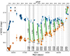 |
Fig. 1. Light curves of SDSS J1001+5027 in the r band and 29 spectroscopic epochs. The large circles/squares with black borders represent LT-HCT-PS magnitudes, while the small semi-transparent circles and squares describe Gaia-ZTF magnitudes (see main text for details). The vertical dotted lines show 25 epochs of spectroscopic observations with LT/SPRAT, leading to ten pairs of AB spectra separated by the time delay of the system (green arrows and horizontal green bars). For these AB pairs, the r-band magnitude offsets are highlighted with vertical green bars. The dashed vertical lines show four epochs of auxiliary spectroscopy (see Appendix B). |
We usually took 4 × 600 s spectroscopic exposures at each observation epoch, covering a wavelength range from 3950 to 8100 Å with a resolving power of 350 (Δλ ∼ 18 Å at the centre of the spectrum). The slit width and position angle were 1 8 (4 pixel) and 122° (or 302°), so it was oriented along the line joining both quasar images. A Xe arc lamp exposure and a standard star were used for wavelength calibration and instrument response correction, respectively. The spectroscopic observations were generally accompanied by 2 × 250 s photometric exposures with IO:O in the SDSS r band. These IO:O exposures allowed us to extract quasar image magnitudes (e.g. Gil-Merino et al. 2018) that were used to calibrate the SPRAT spectra and follow up on the r-band variability of the two quasar images. Our spectroscopic data reduction is fully described in Appendix A.
In Figure 1, the large circles and squares with black borders show all LT/IO:O magnitudes between 2013 and 2025, along with magnitudes from the 2.0 m Himalayan Chandra Telescope (HCT) in 2010–2011 (Rathna Kumar et al. 2013) and the Pan-STARRS (PS; Flewelling et al. 2020) database1 at four epochs. Gaia2 (Prusti et al. 2016) and the Zwicky Transient Facility3 (ZTF; Masci et al. 2019) brightness records in 2014–2017 and 2018–2024, respectively, are also plotted in Figure 1 using small semi-transparent circles and squares. Red magnitudes from telescopes other than the LT were shifted to the LT r-band system. For the most relevant spectro-photometric data of A and B (see the green arrows in Figure 1), the time separations between A and B are highlighted with horizontal green bars, whereas the magnitude offsets between A and B are highlighted with vertical green bars.
4. Pairs of AB spectra separated by the time delay
We obtained ten pairs of AB spectra separated by dt ∼ Δt (see the horizontal green bars in Figure 1)4, which are displayed in Figure 2. Each AB pair corresponds to image spectra at the same emission time, so differences between them are due to differential astrophysical effects. Both differential dust extinction and differential macrolens magnification are expected to be constant over time, while differential microlensing effects may vary with time. Thus, chromatic microlensing variability of SDSS J1001+5027 is caught in action in Figure 2. The spectral differences between A and B have undergone a clear chromatic evolution over the last 10 years, starting with image B being fainter and redder than image A, and ending with image B being brighter and bluer than image A.
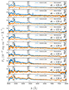 |
Fig. 2. Pairs of time-delay-separated AB spectra. Each pair consists of the spectrum of the leading image A at a first epoch and the spectrum of the trailing image B at a second epoch separated by dt from the first. |
4.1. Emission lines
The SPRAT wavelength range completely covers only the C IVλ1549 and C III]λ1909 emissions. These two emission lines have complex profiles. The blue wing of the C IV line is significantly affected by absorption features in the BAL quasar (e.g. Misawa et al. 2018), and the C III] line profile has two blue-wing excesses related to Si III]λ1892 and Al IIIλ1857 emissions. Thus, we focused on the cores of the C IV and C III] emission lines. The core of each emission line was defined as the spectral region within the rest-frame velocity interval of [ − 1000, +1000] km s−1, so the line core flux comes mainly from a large region unaffected by microlensing. This corresponds to the narrow line region and the outer parts of the broad line region.
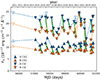 |
Fig. 3. Fluxes of carbon emission line cores. In addition to the measurements from the LT/SPRAT spectra (filled triangles), fluxes associated with the auxiliary spectra are shown (open triangles; see Appendix B). |
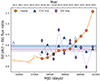 |
Fig. 4. Flux ratios for the cores of the C IV and C III] emission lines. The filled purple diamonds and filled blue triangles represent delay-corrected C IV and C III] line-core flux ratios, respectively, and the horizontal dashed lines and strips describe the average values and their uncertainties (purple for C IV and blue for C III]). The open purple diamonds (C IV) and open blue triangles (C III]) represent single-epoch measurements from auxiliary spectra (see Appendix B). For comparison, we also show the long-term evolution of the delay-corrected r-band flux ratio (filled circles), along with a few single-epoch values before 2016 (open circles). |
The line core flux for each carbon ion is shown in Figure 3. The large scatter in the C IV flux of the two quasar images most probably does not have a physical origin but is due to large calibration uncertainties near the blue edge of the spectrograph (see Appendix A). In addition, the delay-corrected B/A flux ratios for the C IV and C III] line cores (filled purple diamonds and filled blue triangles in Figure 4) show considerable dispersions around their average values (horizontal dashed purple and blue lines in Figure 4). Since there is no apparent long-term variability, we assumed that the observed dispersions are dominated by calibration noise, and estimated delay-corrected line-core flux ratios of 0.761 ± 0.023 (C IV) and 0.792 ± 0.014 (C III]). These two estimates can be interpreted as the product between the macrolens flux ratio and the extinction ratio at the central wavelength of each emission line. However, the two measures are consistent with each other and with the single-epoch flux ratio at near-IR wavelengths (0.787 ± 0.05 in the K band at 21 200 Å; Rusu et al. 2016), suggesting that dust extinction is not appreciably affecting large regions containing carbon ions and ∼0.79 is a good proxy of the macrolens flux ratio.
4.2. Continuum
The delay-corrected spectral flux ratio is depicted in Figure 5. In this figure, for comparison purposes, we also show the single-epoch spectral flux ratio from auxiliary spectra on 1 March 2011 (Gemini North/GMOS; black line) and 3 April 2022 (Keck/LRIS; deep purple line). These Gemini North-Keck data are presented in Appendix B. Figures 4 and 5 also include the delay-corrected r-band flux ratio (filled circles). This broadband ratio is primarily associated with continuum emission and has increased monotonically over the past nine years. Additionally, the continuum slope in the delay-corrected spectral flux ratio has also changed over that time period, undergoing a drastic change in 2025 (cyan line at the top of Figure 5).
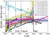 |
Fig. 5. Delay-corrected spectral flux ratio of SDSS J1001+5027. The delay-corrected r-band flux ratio (filled circles), and the single-epoch spectral flux ratio from Gemini North/GMOS (black line) and Keck/LRIS (deep purple line) are also shown. The three horizontal strips correspond to the C IV (purple), C III] (blue), and K-band (grey) flux ratios (see the end of Section 4.1), and are used to highlight the macrolens flux ratio. |
To understand the physics behind the observed evolution (changes) of the continuum, which is assumed to mainly come from the accretion disc, we considered our proxy of the macrolens flux ratio (∼0.79; see the horizontal strips in Figure 5). At the beginning of the monitoring period, the B image was de-magnified (relative to A) by dust extinction effects; it then underwent microlensing-induced changes over the last nine years. The delay-corrected flux ratio at ∼6200 Å (r band) increased noticeably in the period 2022–2025, while it increased considerably more at the shortest wavelengths and barely changed at the longest ones (see Figure 5). The blue portion of the spectrum of image B arises from inner rings of the accretion disc and was magnified more by microlensing than the red portion arising from more external rings. This recent chromatic microlensing episode led to a changing-look of the (delay-corrected) spectral flux ratio. At present, image B is brighter and bluer than A, just the opposite of what was observed in time-delay-separated AB spectra in the first monitoring years (see Figure 2).
5. Conclusions and discussion
One of the main aims of the GLENDAMA project was to detect microlensing-induced quasar chromatic variablity through the analysis of pairs of optical spectroscopic observations of a double quasar separated by the time delay between its two images (Gil-Merino et al. 2018). Here we have presented a long-term spectro-photometric follow-up of SDSS J1001+5027 with the LT, leading to flux ratios between quasar images that are not affected by quasar intrinsic variability. The delay-corrected r-band flux ratio has increased significantly over recent years and the continuum slope in the delay-corrected spectral flux ratio has changed dramatically in the last year of monitoring. These two results suggest that the source quasar is passing through a region of high microlensing magnification (e.g. crossing a microlensing caustic).
Although microlensing-induced chromatic variations in lensed quasars were theoretically predicted long ago (Wambsganss & Paczynski 1991), they have so far only been confidently identified in one quadruply imaged quasar (the Einstein Cross; e.g. Eigenbrod et al. 2008b). In this lens system, the lensing galaxy is located at a very low redshift and the cadence of strong microlensing variations is relatively high. In fact, multi-band light curves of the Einstein Cross over a period of 14 years provided a detailed description of several microlensing chromatic variations and compelling evidence for a double caustic-crossing event (Goicoechea et al. 2020). In this paper, we performed the complicated task of disentangling intrinsic variability, dust extinction, and microlensing effects (e.g. Yonehara et al. 2008) in the doubly imaged quasar SDSS J1001+5027, unambiguously detecting microlensing chromatic variability. Detailed monitoring of this ongoing microlensing event with X-ray, UV, optical, and IR facilities offers us a unique opportunity to improve our understanding of the structure of quasars (e.g. Vernardos et al. 2024).
Quasar images barely vary (if at all) at optical wavelengths on a time scale of ∼5 d.
Acknowledgments
We thank the referee for drawing our attention to several details. We also thank the staff of the Liverpool Telescope (LT) for a kind interaction. The LT is operated on the island of La Palma by Liverpool John Moores University in the Spanish Observatorio del Roque de los Muchachos of the Instituto de Astrofísica de Canarias with financial support from the UK Science and Technology Facilities Council. This long-term research has been supported by the University of Cantabria and several research grants, including the grant PID2020-118990GB-I00 funded by MCIN/AEI/10.13039/501100011033.
References
- Eigenbrod, A., Courbin, F., Sluse, D., Meylan, G., & Agol, E. 2008a, A&A, 480, 647 [NASA ADS] [CrossRef] [EDP Sciences] [Google Scholar]
- Eigenbrod, A., Courbin, F., Meylan, G., et al. 2008b, A&A, 490, 933 [NASA ADS] [CrossRef] [EDP Sciences] [Google Scholar]
- Filippenko, A. V. 1982, PASP, 94, 715 [Google Scholar]
- Fitzpatrick, M., Placco, V., Bolton, A., et al. 2024, arXiv e-prints [arXiv:2401.01982] [Google Scholar]
- Flewelling, H. A., Magnier, E. A., Chambers, K. C., et al. 2020, ApJS, 251, 7 [NASA ADS] [CrossRef] [Google Scholar]
- Gil-Merino, R., Goicoechea, L. J., Shalyapin, V. N., & Oscoz, A. 2018, A&A, 616, A118 [NASA ADS] [CrossRef] [EDP Sciences] [Google Scholar]
- Goicoechea, L. J., Artamonov, B. P., Shalyapin, V. N., et al. 2020, A&A, 637, A89 [NASA ADS] [CrossRef] [EDP Sciences] [Google Scholar]
- Inada, N., Oguri, M., Shin, M.-S., et al. 2012, AJ, 143, 119 [Google Scholar]
- Masci, F. J., Laher, R. R., Rusholme, B., et al. 2019, PASP, 131, 018003 [Google Scholar]
- Misawa, T., Inada, N., Oguri, M., et al. 2018, ApJ, 854, 69 [Google Scholar]
- Moravec, E. A., Hamann, F., Capellupo, D. M., et al. 2017, MNRAS, 468, 4539 [NASA ADS] [CrossRef] [Google Scholar]
- Oguri, M., Inada, N., Hennawi, J. F., et al. 2005, ApJ, 622, 106 [Google Scholar]
- Piascik, A. S., Steele, I. A., Bates, S. D., et al. 2014, Proc. SPIE, 9147, 91478H [Google Scholar]
- Prusti, T., de Bruijne, J. H. J., Brown, A. G. A., et al. 2016, A&A, 595, A1 [NASA ADS] [CrossRef] [EDP Sciences] [Google Scholar]
- Rathna Kumar, S., Tewes, M., Stalin, C. S., et al. 2013, A&A, 557, A44 [NASA ADS] [CrossRef] [EDP Sciences] [Google Scholar]
- Rusu, C. E., Oguri, M., Minowa, Y., et al. 2016, MNRAS, 458, 2 [Google Scholar]
- Schild, R. E., & Smith, R. C. 1991, AJ, 101, 813 [Google Scholar]
- Shajib, A. J., Vernardos, G., Collett, T. E., et al. 2024, Space Sci. Rev., 220, 87 [CrossRef] [Google Scholar]
- Shalyapin, V. N., & Goicoechea, L. J. 2014, A&A, 568, A116 [NASA ADS] [CrossRef] [EDP Sciences] [Google Scholar]
- Sluse, D., Hutsemékers, D., Courbin, F., Meylan, G., & Wambsganss, J. 2012, A&A, 544, A62 [NASA ADS] [CrossRef] [EDP Sciences] [Google Scholar]
- Steele, I. A., Smith, R. J., Rees, P. C., et al. 2004, Proc. SPIE, 5489, 679 [NASA ADS] [CrossRef] [Google Scholar]
- van Dokkum, P. G. 2001, PASP, 113, 1420 [Google Scholar]
- Vanden Berk, D. E., Wilhite, B. C., Kron, R. G., et al. 2004, ApJ, 601, 692 [Google Scholar]
- Vernardos, G., Sluse, D., Pooley, D., et al. 2024, Space Sci. Rev., 220, 14 [NASA ADS] [CrossRef] [Google Scholar]
- Wambsganss, J., & Paczynski, B. 1991, AJ, 102, 864 [NASA ADS] [CrossRef] [Google Scholar]
- Yonehara, A., Hirashita, H., & Richter, P. 2008, A&A, 478, 95 [NASA ADS] [CrossRef] [EDP Sciences] [Google Scholar]
Appendix A: Spectoscopic data reduction
The LT data reduction pipeline removed low-level instrumental signatures through bias and dark current subtraction, and flat-fielding. Additionally, we cleaned cosmic rays using a Python version of L.A.Cosmic algorithm (van Dokkum 2001) called Astro-SCRAPPY5 and carried out other standard calibration procedures in a NOIRLab IRAF v2.18 environment (Fitzpatrick et al. 2024). The outputs are wavelength-calibrated sky-subtracted 2D spectra.
A.1. Source spectra extraction
After the initial spectral reduction (see above), the 1D spectrum of the standard star was extracted by summing fluxes along the slit for each wavelength bin. However, the extraction of 1D spectra of both quasar images is a more complex task (e.g. Shalyapin & Goicoechea 2014). For the double quasar, the light distribution along the slit was modelled as two Gaussian-shaped profiles with the same width and separated by 2 928 (see Sect. 2). This spatial model depends on four parameters: the Gaussian width, the two Gaussian amplitudes, and the position of the centre of the Gaussian profile for the image A. In a first iteration, we fitted the four free parameters of the spatial model to the fluxes along the slit for each wavelength bin. The Gaussian width and the position of A were then approximated by low-degree polynomial functions of the observed wavelength, and in a second iteration, these two parameters were fixed to their polynomial values, fitting only the two Gaussian amplitudes. The spatial integration of the Gaussian profiles at each wavelength bin led to the 1D spectra of A and B.
A.2. Flux calibration issues
We paid special attention to the instrument response functions from observations of the standard star and the corrections of chromatic slit losses caused by differential atmospheric refraction (DAR). These calibration issues are described here below.
The SPRAT response function on a given night was initially estimated from standard star data for that night, and the response functions at all SPRAT observation epochs are shown in Figure A.1. However, the extraction of the 1D stellar spectra is not reliable at the low-sensitivity spectral edges, probably leading to biases in the instrument responses at the shortest and longest wavelengths. To analyse possible biases, we took as reference the 170405 response function (corresponding to good observing conditions on 5 April 2017; see the blue solid line in Figure A.1), and then calculated the relative responses (dividing by the reference) and multiplied them by appropriate factors so that they equal 1 at 6200 Å. These normalised relative responses are plotted in Figure A.2. Due to the evidence of instrumental artefacts at 4000–4500 and 7500–8000 Å, we fitted second degree polynomials to the normalised relative responses in the central spectral region (4500–7500 Å) and extrapolated these central fits to the spectral edges (dashed lines in Figure A.2). Hence, for each night, the normalised response function was finally obtained as the product of the reference response and the corresponding polynomial function.
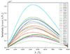 |
Fig. A.1. SPRAT response functions at the 25 observation epochs. We use labels YYMMDD, where YY, MM, and DD represent the last two digits of the year, the month, and the day of the month, respectively. These YYMMDD labels are also used in Figures A.2, A.4, and A.5. |
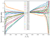 |
Fig. A.2. Normalised relative responses (see main text). The dashed lines are second-degree polynomial fits to the normalised relative responses in the central spectral region (4500–7500 Å), which are extrapolated to both spectral edges. |
The LT is a robotic telescope, and it is difficult to place sources on the slit axis by an automatic unattended operation. Thus, the quasar images are expected not to be perfectly centred on the slit. To estimate their position across the slit at each observation epoch, we analysed the corresponding through-slit acquisition frame (see Figure A.3). First, we payed attention to the transverse brightness distribution of the background light far from the quasar and found the position of the slit axis on the SPRAT CCD (y = 0). After subtracting the background, we then determined the acquisition transverse offset δy of the quasar images by fitting an off-axis Gussian profile to the light distribution across the slit in the region where the quasar images are located. The two quasar images are assumed to be shifted by δy at a reference wavelength of 6200 Å, which is close to that of maximum sensitivity of the SPRAT CCD (Piascik et al. 2014) and to the central wavelength of the r passband (the final flux calibration is based on photometric measurements with IO:O in the r band; see below).
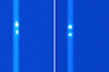 |
Fig. A.3. Through-slit acquisition frames on 9 April 2019 (left) and 2 December 2015 (right). In the left panel, the two quasar images are clearly off-axis. |
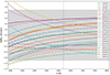 |
Fig. A.4. Chromatic offsets of quasar images across the slit for each observation night. These offsets are due to off-axis acquisitions at 6200 Å and DAR. The horizontal dashed line represents the slit axis, while the vertical side of the grey strip corresponds to the slit width of 1 |

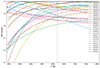 |
Fig. A.5. Chromatic slit losses for each observation night. Slit losses on a given night are estimated using the offsets for that night (see Figure A.4) and a circular Gaussian source with an observationally motivated width (see main text). |
An additional problem is the differential atmospheric refraction. At each observation epoch, the slit was oriented along the line joining the two quasar images (see Sect. 3), so its position angle did not coincide with the parallactic angle. This deviation from the parallactic angle caused DAR, which shifted both images across the slit and increased the light (slit) losses, especially at blue wavelengths (Filippenko 1982). The LT is not equipped with a DAR corrector, and thus we developed a procedure to numerically correct these wavelength-dependent slit losses leading to spectral artefacts. Our procedure relied on the analysis by Filippenko (1982), who provided a method to derive DAR-induced offsets in function of the deviation from the parallactic angle, the airmass value, and the weather conditions.
The DAR offsets were calculated relative to the reference wavelength (6200 Å), and results at all epochs are shown in Figure A.4. For this reference wavelength, the quasar images are not on the slit axis, but shifted across the slit by the δy offsets inferred from the through-slit acquisition frames (see above). Additionally, we estimated the chromatic slit losses at all epochs for a circular Gaussian source with width σ, using σ values obtained by analysing the through-slit acquisition frames (see Figure A.5). After correcting for instrument responses and slit losses, we also used IO:O r-band fluxes to properly calibrate the quasar spectra.
Appendix B: Auxiliary spectra
In addition to the set of 25 LT/SPRAT spectra, we considered spectroscopic observations from other facilities at four different epochs (vertical dashed lines in Figure 1). Although these data can only yield simultaneous spectra of A and B at each observation epoch, and therefore the B/A spectral flux ratio could be affected by intrinsic variations, the observations were done using 8–10 m class telescopes and complement our LT monitoring programme.
We downloaded and processed archive data of the Gemini North Telescope6 (GMOS instrument, 1 March 2011) and the Keck Telescope7 (LRIS instrument, 3 April 2022). These spectroscopic data allowed us to extract spectra for the two quasar images extending up to 9000–10 000 Å (see Figure B.1). We also used Subaru Telescope/HDS spectra on 27 January 2016 and 19 January 2017 that were obtained by Misawa et al. (2018) and cover the spectral region around the C IV emission line.
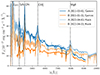 |
Fig. B.1. Auxiliary spectra of SDSS J1001+5027 from near-UV to near-IR. |
All Figures
|
Fig. 1. Light curves of SDSS J1001+5027 in the r band and 29 spectroscopic epochs. The large circles/squares with black borders represent LT-HCT-PS magnitudes, while the small semi-transparent circles and squares describe Gaia-ZTF magnitudes (see main text for details). The vertical dotted lines show 25 epochs of spectroscopic observations with LT/SPRAT, leading to ten pairs of AB spectra separated by the time delay of the system (green arrows and horizontal green bars). For these AB pairs, the r-band magnitude offsets are highlighted with vertical green bars. The dashed vertical lines show four epochs of auxiliary spectroscopy (see Appendix B). |
| In the text | |
|
Fig. 2. Pairs of time-delay-separated AB spectra. Each pair consists of the spectrum of the leading image A at a first epoch and the spectrum of the trailing image B at a second epoch separated by dt from the first. |
| In the text | |
|
Fig. 3. Fluxes of carbon emission line cores. In addition to the measurements from the LT/SPRAT spectra (filled triangles), fluxes associated with the auxiliary spectra are shown (open triangles; see Appendix B). |
| In the text | |
|
Fig. 4. Flux ratios for the cores of the C IV and C III] emission lines. The filled purple diamonds and filled blue triangles represent delay-corrected C IV and C III] line-core flux ratios, respectively, and the horizontal dashed lines and strips describe the average values and their uncertainties (purple for C IV and blue for C III]). The open purple diamonds (C IV) and open blue triangles (C III]) represent single-epoch measurements from auxiliary spectra (see Appendix B). For comparison, we also show the long-term evolution of the delay-corrected r-band flux ratio (filled circles), along with a few single-epoch values before 2016 (open circles). |
| In the text | |
|
Fig. 5. Delay-corrected spectral flux ratio of SDSS J1001+5027. The delay-corrected r-band flux ratio (filled circles), and the single-epoch spectral flux ratio from Gemini North/GMOS (black line) and Keck/LRIS (deep purple line) are also shown. The three horizontal strips correspond to the C IV (purple), C III] (blue), and K-band (grey) flux ratios (see the end of Section 4.1), and are used to highlight the macrolens flux ratio. |
| In the text | |
|
Fig. A.1. SPRAT response functions at the 25 observation epochs. We use labels YYMMDD, where YY, MM, and DD represent the last two digits of the year, the month, and the day of the month, respectively. These YYMMDD labels are also used in Figures A.2, A.4, and A.5. |
| In the text | |
|
Fig. A.2. Normalised relative responses (see main text). The dashed lines are second-degree polynomial fits to the normalised relative responses in the central spectral region (4500–7500 Å), which are extrapolated to both spectral edges. |
| In the text | |
|
Fig. A.3. Through-slit acquisition frames on 9 April 2019 (left) and 2 December 2015 (right). In the left panel, the two quasar images are clearly off-axis. |
| In the text | |
|
Fig. A.4. Chromatic offsets of quasar images across the slit for each observation night. These offsets are due to off-axis acquisitions at 6200 Å and DAR. The horizontal dashed line represents the slit axis, while the vertical side of the grey strip corresponds to the slit width of 1 |
| In the text | |
|
Fig. A.5. Chromatic slit losses for each observation night. Slit losses on a given night are estimated using the offsets for that night (see Figure A.4) and a circular Gaussian source with an observationally motivated width (see main text). |
| In the text | |
|
Fig. B.1. Auxiliary spectra of SDSS J1001+5027 from near-UV to near-IR. |
| In the text | |
Current usage metrics show cumulative count of Article Views (full-text article views including HTML views, PDF and ePub downloads, according to the available data) and Abstracts Views on Vision4Press platform.
Data correspond to usage on the plateform after 2015. The current usage metrics is available 48-96 hours after online publication and is updated daily on week days.
Initial download of the metrics may take a while.