| Issue |
A&A
Volume 702, October 2025
|
|
|---|---|---|
| Article Number | A41 | |
| Number of page(s) | 32 | |
| Section | Cosmology (including clusters of galaxies) | |
| DOI | https://doi.org/10.1051/0004-6361/202452910 | |
| Published online | 07 October 2025 | |
No rungs attached: A distance-ladder-free determination of the Hubble constant through type II supernova spectral modelling
1
Max-Planck-Institut für Astrophysik, Karl-Schwarzschild-Str. 1, 85741 Garching, Germany
2
Technische Universität München, TUM School of Natural Sciences, Physics Department, James-Franck-Straße 1, 85748 Garching, Germany
3
Heidelberg Institute for Theoretical Studies, Schloss-Wolfsbrunnenweg 35, 69118 Heidelberg, Germany
4
Aix Marseille Univ, CNRS, CNES, LAM, Marseille, France
5
European Southern Observatory, Karl-Schwarzschild-Straße 2, 85748 Garching, Germany
6
Exzellenzcluster ORIGINS, Boltzmannstr. 2, 85748 Garching, Germany
7
Department of Physics and Astronomy, Michigan State University, East Lansing, MI 48824, USA
8
Department of Computational Mathematics, Science, and Engineering, Michigan State University, East Lansing, MI 48824, USA
9
Astrophysics Research Centre, School of Mathematics and Physics, Queen’s University Belfast, Belfast BT7 1NN, UK
10
GSI Helmholtzzentrum für Schwerionenforschung, Planckstraße 1, 64291 Darmstadt, Germany
11
Department of Physics, Duke University, Durham, NC 27708, USA
12
University Claude Bernard Lyon 1, IUF, IP2I Lyon, 69622 Villeurbanne, France
⋆ Corresponding author: This email address is being protected from spambots. You need JavaScript enabled to view it.
Received:
6
November
2024
Accepted:
19
May
2025
Abstract
Context. The ongoing discrepancy among Hubble constant (H0) estimates obtained through local distance ladder methods and early Universe observations poses a significant challenge to the ΛCDM model, suggesting potential new physics. Type II supernovae (SNe II) offer a promising technique for determining H0 in the Local Universe independently of the traditional distance ladder approach, opening up a complimentary path for testing this discrepancy.
Aims. We aim to provide the first H0 estimate using the tailored expanding photosphere method (EPM) applied to SNe II, made possible by recent advancements in spectral modelling that enhance its precision and efficiency.
Methods. Our tailored EPM measurement utilises a spectral emulator to interpolate between radiative transfer models calculated with TARDIS, allowing us to fit SN spectra efficiently and derive self-consistent values for luminosity-related parameters. We applied the method to a set of public data for ten SNe II at redshifts between 0.01 and 0.04.
Results. Our analysis demonstrates that the tailored EPM allows us to obtain H0 measurements with a precision comparable to the most competitive established techniques, even when applied to literature data that are not designed for cosmological applications. We find an independent H0 value of 74.9 ± 1.9 (stat) km s−1 Mpc−1, which is consistent with most current local measurements. Considering dominant sources of systematic effects, we conclude that our systematic uncertainty is comparable to (or less than) the current statistical uncertainty.
Conclusions. This proof-of-principle study highlights the potential of the tailored EPM as a robust and precise tool for investigating the Hubble tension independently of the local distance ladder. Observations of SNe II tailored to H0 estimations could make this an even more powerful tool by improving the precision and allowing us to improve our understanding of the systematic uncertainties and how to control them.
Key words: distance scale / radiative transfer / supernovae: general
© The Authors 2025
 Open Access article, published by EDP Sciences, under the terms of the Creative Commons Attribution License (https://creativecommons.org/licenses/by/4.0), which permits unrestricted use, distribution, and reproduction in any medium, provided the original work is properly cited.
This article is published in open access under the Subscribe to Open model.
Open access funding provided by Max Planck Society.
1. Introduction
Advancements made in the past decade in terms of cosmic distance measurements have brought forward a persistent discrepancy between the Hubble constant (H0) values when estimated through different means: currently, the community faces a 5.8σ tension between the H0 measured directly from redshifts and distances in the local universe (73.17 ± 0.86 km s−1 Mpc−1), based on the SH0ES analysis (Riess et al. 2022; Breuval et al. 2024) employing the Cepheid period-luminosity relation and type Ia supernovae (SNe Ia), and the same parameter estimated through the cosmic microwave background (CMB) assuming a ΛCDM cosmology (67.4 ± 0.5 km s−1 Mpc−1, Planck Collaboration I 2020).
The Hubble tension between the local universe and CMB estimates currently constitutes one of the biggest challenges for the successful ΛCDM model, potentially hinting at new physics. Possible explanations include early dark energy (Poulin et al. 2019; Smith et al. 2020a; Herold & Ferreira 2023), new neutrino physics (Kreisch et al. 2020; Berbig et al. 2020), interaction between dark matter and dark energy (Wang et al. 2016; Pan & Yang 2024), as recently reviewed by Di Valentino et al. (2021), Verde et al. (2024), or in the H0 Olympics (Schöneberg et al. 2022).
The Hubble tension, which first emerged between the SH0ES (Cepheids and SNe Ia) and Planck (CMB) observations, has been confirmed by other methods for the local and distant measurements. The lower value from the CMB is supported by independent measurements from Wilkinson Microwave Anisotropy Probe (WMAP; Hinshaw et al. 2013), Atacama Cosmology Telescope (ACT; Aiola et al. 2020), and South Pole Telescope (SPT; Dutcher et al. 2021). Similar results have been obtained through baryonic acoustic oscillations (BAOs), even when calibrated through CMB-independent means such as Big Bang nucleosynthesis (see e.g. Abbott et al. 2018; Schöneberg et al. 2019).
In the local universe, mass over-densities induce local disturbances over the pure space expansion (e.g. Cosmicflows-4; Tully et al. 2023) and distance indicators reaching into the Hubble flow are required (e.g. Sandage & Tammann 1974). The local distance ladder has been reduced over the past decades to three steps: geometric distances through parallaxes or detached eclipsing binaries, calibration of intermediate distance indicators (Cepheid stars, TRGB stars, Mira variables), and the subsequent calibration of luminous objects in the Hubble flow (SNe Ia, galaxies, etc.). Various recent versions of the local distance ladder agree with the Cepheid-SN Ia analysis and point to a higher value of H0: similar H0 values are obtained when Cepheids are replaced by distances to Mira variables for the second rung (Huang et al. 2020, 2024), or SNe Ia are replaced by surface brightness fluctuations (Blakeslee et al. 2021) or Tully-Fisher distances (Schombert et al. 2020; Tully et al. 2023) for the third rung.
A notable exception to this trend was reported by Freedman et al. (2019, 2020) and Freedman (2021), who used the tip of the red giant branch (TRGB) technique for the second rung and derived a Hubble constant (H0 = 69.8 ± 1.71 km s−1 Mpc−1) consistent with both the CMB and SH0ES. Other, independent TRGB analyses, however, have yielded H0 values closer to SH0ES (e.g. Anand et al. 2022; Scolnic et al. 2023; Uddin et al. 2024).
Freedman et al. (2025) presented an analysis based on JWST observations, where they also reported a lower H0 value (69.96 ± 1.53 km s−1 Mpc−1) by combining estimates from Cepheids, the J-band asymptotic giant branch method (JAGB, Madore & Freedman 2020), and the TRGB method, all applied along the same distance ladder with identical SN Ia calibrator hosts (Lee et al. 2025; Hoyt et al. 2024). Shortly afterwards, the SH0ES team presented an estimate based on an extended set of calibrator hosts observed by JWST, finding H0 = 72.6 ± 2.0 km s−1 Mpc−1 (Riess et al. 2024), and suggesting that selection effects in calibrator host galaxies explain the discrepancy.
These inconsistencies highlight the importance of assessing systematic effects in the distance ladder. For example, the effect of varying metallicity on the Cepheid (Breuval et al. 2022) and TRGB distances (Hoyt 2023; Madore & Freedman 2024) is frequently revisited in the literature. Furthermore, it was shown that the treatment of reddening can also cause systematic offsets in the calibration of the Cepheid period-luminosity relation (e.g. Mörtsell et al. 2022a,b), just as stellar variability may cause variations in the TRGB absolute brightness (Anderson et al. 2024a; Koblischke & Anderson 2024).
To resolve the ongoing Hubble tension, it is essential to address any systematic effects or find methods with independent systematics. A distance indicator bypassing the calibration through a distance ladder and based on known physics is ideal for a cross-check with independent systematics. Three promising methods to measure individual distances in the Hubble flow have recently been discussed: megamasers around galaxy nuclei, which provide a geometric distance (e.g. Reid et al. 2019), time delay cosmography of lensed quasars or SNe (e.g. Suyu et al. 2017), and the expanding photosphere method with type II supernovae (SNe II). All methods currently suffer from small number statistics and have individual challenges.
Pesce et al. (2020) analysed a sample of five masers. Apart from the currently small sample size, megamasers have not been observed far into the Hubble flow and, hence, they suffer from high uncertainties due to peculiar velocities (Pesce et al. 2020).
Time-delay cosmography has been performed with eight lensed quasars (Chen et al. 2019; Wong et al. 2020, 2024; Shajib et al. 2020; Millon et al. 2020; Birrer et al. 2020). Individual distances can be determined to about 4% in the best cases. Kelly et al. (2023), Grillo et al. (2024) and Pascale et al. (2025) estimated H0 based on SNe lensed by galaxy clusters, while efforts are ongoing to perform similar measurements using SNe behind galaxy-scale lens systems (see, e.g. Suyu et al. 2020). Time delay lensing measures distances well beyond the local universe (source and lens redshifts are typically at z ≳ 0.5), and depends to some degree on the assumed cosmological model (e.g. Taubenberger et al. 2019). The H0 uncertainties depend significantly on the assumed lens density profile, which is required to break the mass-sheet degeneracy. Without such assumptions, the H0 uncertainties increase to ∼8% for a sample of seven lenses (Birrer et al. 2020), unless there are spatially resolved stellar kinematics of the lens galaxies available (e.g. Shajib et al. 2023; Yıldırım et al. 2023).
Type II supernovae, resulting from the collapse of massive (≥8 M⊙) hydrogen-rich stars, have a long history as distance indicators. Several methods, varying in data requirements and complexity, have been explored for this purpose, as reviewed by de Jaeger & Galbany (2024). Among these techniques, three rely on the standardisation of supernova brightnesses, analogous to SN Ia cosmology: the standardised candle method (SCM; Hamuy & Pinto 2002) correlates the luminosity during the light curve plateau phase with the expansion velocity at a fixed time since explosion, typically around 50 days post-explosion. The photospheric magnitude method (PMM; Rodríguez et al. 2014, 2019) is a generalisation of SCM that directly utilises measurements from multiple epochs, rather than interpolating or extrapolating them to a single epoch. The photometric colour method (PCM; de Jaeger et al. 2015, 2017) calibrates SN II magnitudes using their decline rate in the photospheric phase (denoted as s2 in the literature, see e.g. Anderson et al. 2014), solely requiring photometric information. Each of these methods needs to be calibrated with other distance indicators (e.g. Cepheids) and is a component of the distance ladder (e.g. de Jaeger et al. 2020a, 2022). So far, only the SCM and PMM have been used for inferring the Hubble constant. Notable recent results include those of de Jaeger et al. (2022), who derived  (stat) ±1.5 (sys) km s−1 Mpc−1 based on SCM, and Rodríguez et al. (2019), who obtained values ranging from
  to
to  km s−1 Mpc−1 (stat) using PMM, depending on the choice of photometric band and RV.
The expanding photosphere method (EPM; Kirshner & Kwan 1974) provides an alternative path, bypassing the need for a standardisation procedure: it relies on a physical model for the photospheric emission and the expansion of the ejecta to relate the observed flux to intrinsic luminosity, thereby providing direct distances to SNe II.
Hubble constant determinations with the EPM have been attempted over several decades (see e.g. Schmidt et al. 1992, 1994; Eastman et al. 1996; Gall et al. 2016; Dhungana et al. 2024). The first EPM H0 estimate was based on two SNe (Kirshner & Kwan 1974) and assumed that the SN radiates as a blackbody – a natural first approximation. However, Wagoner (1981) later demonstrated that this assumption did not capture the full complexity of the emission process. The radiation continuum is formed far below the photosphere due to the dominance of scattering opacity, leading to a diluted continuum. The dilution factor of ξ was introduced to incorporate the deviations from blackbody radiation. Non-LTE models of Eastman et al. (1996) and Dessart & Hillier (2005) have shown that this parameter depends primarily on the temperature and provided the necessary tables of dilution factors, thereby improving the distance estimation accuracy. Schmidt et al. (1994) were the first to estimate H0 with the improved EPM. Gall et al. (2018) demonstrated that this method can be used at redshifts up to z = 0.3. The latest H0 estimates through EPM were published by de Jaeger & Galbany (2024) and by Dhungana et al. (2024), deriving  (stat) ±13.46 (sys) and
  (stat), respectively, both using dilution factors from Dessart & Hillier (2005). Both studies emphasise that the choice of dilution factors introduces significant systematic uncertainties in the analysis.
Tabulated dilution factors present a clear limitation for the EPM. Dilution factors can vary considerably as the SN luminosity depends not only on temperature but, for example, also on the ejecta density profile. This limitation can lead to systematic biases in individual distance estimates if the models used for dilution factors systematically differ from the actual properties of the observed SNe. In fact, differences in the ejecta density structure of the underlying SN models are one of the reasons for the significant discrepancies between the dilution factors computed by Eastman et al. (1996) and Dessart & Hillier (2005) (see Vogl et al. 2019).
Dessart & Hillier (2006) emphasised the need to find radiative transfer models that reproduce the SN spectrum at each epoch. By matching models to observations, one ensures that the properties influencing the luminosity, including the density profile, are accurately captured. This approach is known as the tailored EPM (Dessart & Hillier 2006) or the spectral-fitting expanding atmosphere method (SEAM; Baron et al. 2004). While this method improves the accuracy of distance measurements, it is highly time-consuming. Finding suitable models requires calculating many complex radiative transfer simulations, each demanding significant computational resources. Thus, only three SN II spectral time series have been modelled with the goal of measuring distances (Baron et al. 2004; Dessart & Hillier 2006; Dessart et al. 2008). To remedy this situation, we have introduced a spectral emulator approach showcased in Vogl et al. (2020), capable of interpolating radiative transfer models within a pre-defined parameter space in a fraction of the time needed to run a single radiative transfer model. These interpolated models can then be used as an input for distance measurements with the tailored EPM.
Another improvement for the EPM was demonstrated by Vogl et al. (2020): with a precise estimate of the time of explosion (uncertainty of ≲2 d; see Sect. 3.1), the EPM can be applied using even a single spectral epoch to constrain the distance with 10 − 20% precision (or better), as each individual epoch can be fitted for luminosity.
The power of the tailored EPM was tested by applying it on four SN II siblings – SNe II which exploded in the samegalaxy – yielding encouraging consistency (Csörnyei et al. 2023a). Tailored EPM distance estimates are as precise as state-of-the-art techniques, such as those based on Cepheids and TRGB, and yield similar results (Vogl et al. 2020; Csörnyei et al. 2023b). Using the tailored EPM, SNe II are capable of estimating distances in the Hubble flow and provide an independent H0 value with competitive precision.
We present the first H0 estimate using the tailored EPM for SNe II, building on the improvements of Dessart & Hillier (2006) and Vogl et al. (2020). We utilised literature datasets not specifically designed for the tailored EPM and demonstrate that even they can provide the basis for a precise H0 estimation. We performed this analysis as a proof-of-principle to lay the foundation for future studies with dedicated datasets optimised for distance measurements.
This paper is structured as follows: Section 2 introduces the theoretical framework for the tailored EPM and the application to measure H0. Section 3 describes the spectroscopic and photometric data. In Sect. 4, we describe the key analysis steps, including time-of-explosion determination, light-curve interpolation, spectral calibration, and fitting of radiative transfer models. Section 5 connects these steps to derive the ratios of the photospheric angular diameter and photospheric velocities, as well as the extinction, which is crucial for calculating distances. We determined H0 through a joint fit of these ratios in Sect. 6. The results are then discussed in Sect. 7, comparing them with other H0 measurements, exploring systematic uncertainties, and assessing the implications for the ongoing H0 tension. Finally, Sect. 8 provides a summary and suggests directions for future research.
2. Basic principle
2.1. Expanding photosphere method
As with other methods for determining luminosity distances, the EPM relates the observed specific flux to the intrinsic specific luminosity of the object. The relevant equation in the absence of extinction is (e.g. Hogg 1999, Eq. (23)):
 (1)
(1)
Due to the cosmic redshift z, the observed specific flux fλ, obs at observed wavelength λ relates to the luminosity, Lλem, at the emitted wavelength of λem = λ/(1 + z). We can then solve Eq. (1) for the luminosity distance, DL, if we can constrain the SN luminosity.
Assuming spherical symmetry, we express the luminosity in terms of the radius of the emitting region – the photospheric radius Rph – and the specific flux at that radius, fλem, ph:
 (2)
(2)
We can determine fλem, ph by modelling the SN emission based on spectroscopic observations. The photospheric radius can be calculated from the photospheric velocity, vph, using the assumption of homologous expansion:
 (3)
(3)
The photospheric radius at time t in the observer frame is thus the photospheric velocity multiplied by the time since the explosion in the SN frame, (t − t0)/(1 + z) (e.g. Leibundgut et al. 1996; Blondin et al. 2008). It is assumed that, after the prompt acceleration in the explosion, the ejected material moves at a constant velocity for each mass coordinate; the initial radius of the ejected material is considered to be negligible.
The photospheric velocity, finally, can be inferred from Doppler-broadened P-Cygni features. If we knew the time of explosion t0, we could now directly solve Eqs. (1) and (2) for the luminosity distance. In practice, however, the EPM involves an additional step since historically the time of explosion was not well-constrained for most objects.
We circumvent this lack of knowledge by calculating the ratio of Rph and DL as
 (4)
(4)
which is commonly called the photospheric angular diameter θ. This name is misleading, however, because the true angular diameter is calculated using the angular diameter distance, DA, not the luminosity distance DL1.
Finally, we divide the photospheric angular diameter by the photospheric velocity. Using Eq. (3) and the definition of θ we see that this ratio grows linearly with time starting from zero at the time of explosion. The rate of growth is inversely proportional to the distance DL:
 (5)
(5)
If we have measurements of θ/vph from multiple spectroscopic observations, we can thus fit a straight line to the temporal evolution; the time of explosion is then the intercept of the line and the distance is the inverse of the slope. Figure 1 illustrates this basic principle of the EPM.
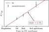 |
Fig. 1. EPM regression principle. The EPM uses multiple spectroscopic observations to measure the ratio of the photospheric angular diameter θ (Eq. (4)) and the photospheric velocity vph for different times. These measurements (shown in blue) fall on a straight line (red). We can determine the SN luminosity distance DL from the inverse of the slope of this line and the time of explosion from the intercept (see Eq. (5)). |
While the general idea is simple, the details of the implementation are complex. We need measurements of the observed specific flux fλ, obs, the photospheric velocities vph, and models for the specific flux at the photosphere fλem, ph to calculate θ/vph values.
Out of the three, only the observed specific flux is straightforward to determine: we simply interpolate the available photometry to the epochs of spectroscopic observations (see Sect. 4.2). The other two (vph and fλem, ph), for the tailored EPM, come from sophisticated radiative transfer models that are optimised to match the spectroscopic observations (Sect. 4.4).
2.2. From distances to the Hubble constant
We use the kinematic expansion of the luminosity distance DL (see e.g. Riess et al. 2004) to relate our EPM distances to the Hubble constant H0:
![Mathematical equation: $$ \begin{aligned} D_\mathrm{L} = \frac{c z}{H_0} \left[1 + \frac{1}{2} (1 - q_0) z - \frac{1}{6} (1 - q_0 - 3q_0^2 + j_0) z^2 + O(z^3)\right]. \end{aligned} $$](/articles/aa/full_html/2025/10/aa52910-24/aa52910-24-eq11.gif) (6)
(6)
We adopt a deceleration parameter q0 = −0.55 and jerk j0 = 1 as in Riess et al. (2016, 2022), corresponding to a flat ΛCDM cosmology with ΩM = 0.3. These values can be measured from high-redshift SNe Ia without requiring an absolute calibration of the SNe through a distance ladder (e.g. Betoule et al. 2014).
The choice of q0 and j0, however, is not critical because we work at relatively low redshifts (≲0.04), where the nonlinear terms in Eq. (6) are ≲3%. For comparison, in their SN Ia sample with a higher mean redshift of 0.07, Riess et al. (2016) find that the uncertainty in q0 only introduces a 0.1% uncertainty in H0.
The final challenge is that the redshift z in Eq. (6) is the true cosmological redshift of the SN host galaxy zcosmo, not the measurable heliocentric redshift. They differ due to peculiar motions of our galaxy and the SN host galaxy (e.g. Davis & Scrimgeour 2014). We can correct for our own motions by transforming the redshift to the CMB rest frame (zCMB) using the well-measured CMB dipole parameters (e.g. Planck Collaboration I 2020). Assuming that we know the host galaxy peculiar velocity vpec, zcosmo is then given by (see e.g. Davis & Scrimgeour 2014):
 (7)
(7)
The challenge lies in determining vpec, which is much harder to quantify than our own peculiar motion. However, observations of big samples of objects can be used to model the large scale flows in the universe. These models then provide approximate peculiar velocities for individual galaxies (see Sect. 4.5).
3. Observational data
3.1. Sample selection
The data for a tailored EPM measurement of H0 have to meet very specific requirements. First, the SNe must have significant redshifts to reduce the impact of peculiar velocities, which remain important even after flow corrections. We only considered SNe at zCMB > 0.01, where peculiar velocities contribute at most a 10% uncertainty in the H0 measurement from a single SN2.
Second, the SNe also need tight constraints on the time of explosion t0 (see Sect. 4.1 for details on this constraint). By excluding SNe with t0 uncertainties over two days, we limited the contribution to the distance uncertainties to about 10% at a representative phase of 20 d. The tight t0 constraints have the added benefit that even objects with only one suitable spectrum can be used.
Third, for a spectrum to be suitable for our purposes, it must meet several criteria. It must be taken within 35 d post-explosion, have accurate relative flux calibration, minimal host contamination, and be sufficiently normal to be modelled with a standard SN II atmosphere without, for example, accounting for circumstellar material (CSM) interaction. The 35 d limit ensures that neglecting time dependence in the excitation and ionisation balance remains a sound approximation, as this assumption becomes less accurate over time (see discussion in Vogl et al. 2019). The other criteria help ensure that the spectral modelling results are physical and less likely to be influenced by limitations in the data or the modelling. Finally, we required photometry in at least two bands to recalibrate the spectra against the photometry (see Sect. 4.3).
While many objects with data published in the literature meet some requirements, very few pass all of them. Our search of WISeREP (Yaron & Gal-Yam 2012)3 and the Open Supernova Catalog (OSC; Guillochon et al. 2017)4 has yielded only four SNe: SN 2003bn, SN 2006it, SN 2010id, and SN 2013fs5. Out of these, SN 2013fs is a borderline case: its early evolution is marked by CSM interaction (Yaron et al. 2017) and it becomes spectroscopically normal (according to our earlier description) only around three weeks post-explosion. We include it as a tentative test whether objects with early CSM interaction can be reliable distance indicators with our approach.
We extended our sample by including SNe without published follow-up data, but with publicly available classification spectra from the advanced Public ESO Spectroscopic Survey for Transient Objects (ePESSTO+) – the successor of the PESSTO program (Smartt et al. 2015). The project classifies transients with apparent magnitudes up to 19.5, which includes normally bright SNe II up to redshifts of around 0.04. The classified objects are usually young with well-constrained explosion epochs, making them suitable for the EPM despite having only one spectrum.
Table 1 summarises the properties of our combined sample of literature objects and ePESSTO+ classification targets including redshifts, peculiar velocities (see Sect. 4.5), and Milky Way extinction values.
Supernova sample for H0 measurement.
3.2. Spectroscopy
We retrieved the spectra for the literature sample from WISeREP and the Open Supernova Catalog. Table A.1 lists their original sources.
We have re-reduced the publicly available ePESSTO+ raw data to ensure uniform data quality from this source. This included flat-fielding, cosmic ray rejection with L.A.Cosmic (van Dokkum 2001), and an optimal, variance-weighted extraction with IRAF’s (Tody 1986, 1993) apall task. The wavelength calibration was performed using arc lamps and verified against night sky lines.
Given the blue colours of early-phase SNe II, second order contamination in EFOSC2 (Buzzoni et al. 1984) was a concern. We thus corrected the ePESSTO+ spectra for it using an adapted version of the method of Stanishev (2007).
For the flux calibration, we constructed sensitivity curves from multiple standard star observations taken close in time to the SN data. We calibrated the spectra using the mean sensitivity curve. Afterwards, we applied a telluric absorption correction using a mean correction function derived from standard star spectra. This was done with the IRAF task telluric, which allowed us to fine-tune the correction by adjusting the wavelength shift and scaling the absorption strengths of the O2 and H2O bands independently6.
In contrast to our re-reduced ePESSTO+ spectra, the literature spectra were not explicitly corrected for second-order contamination. Most were obtained using double-beam spectrographs, cross-dispersed spectrographs, or multiple grisms, which naturally eliminate second-order effects. Similarly, telluric absorption had already been corrected for in the majority of literature spectra. The only exception was SN 2003bn, for which we applied a telluric correction following the same procedure as for the ePESSTO+ spectra.
Our full set of spectra is summarised in Table A.1, with each row corresponding to one spectrum at the specified time (MJD). Before fitting the spectra with radiative transfer models in Sect. 4.4, we also converted the observed wavelengths from air to vacuum using the method described by Ciddor (1996).
3.3. Photometry
The EPM relies on photometric measurements of the observed specific flux fλ, obs to calculate the photospheric angular diameter θ (Eq. (4)) and recalibrate the spectra against the photometry (Sect. 4.3). Table A.1 lists the sources and photometric systems of our photometry.
We retrieved the ZTF photometry from the ZTF forced-photometry service (Masci et al. 2023) and processed it according to the manual, including quality filtering, baseline correction, and validation of flux-uncertainty estimates. For the photometry obtained from literature sources, detailed descriptions of the photometric reduction methods can be found in the original references listed in Table A.1.
All photometric measurements used in this study were obtained through point-spread function (PSF) fitting photometry. For nearly all objects, host-galaxy contamination has been removed by template subtraction. Exceptions are SN 2013fs, for which a low-order polynomial fit was used to subtract the host-galaxy background (Valenti et al. 2016), and SN 2010id, for which host subtraction was likely not performed, given that de Jaeger et al. (2019) applied such corrections primarily to objects located close to their host galaxies, whereas SN 2010id was observed in a remote location.
We used the natural instrument system of the respective surveys whenever possible to avoid problems associated with first-order colour term corrections. The appropriate passbands are from Ganeshalingam et al. (2010) for the KAIT4 and Hicken et al. (2009)7 for the CfA3KEP systems. We adopted the products of the CCD quantum efficiency (QE), the filter transmissions from Bellm et al. (2019), and a standard atmospheric transmission at 1.3 airmass (Doi et al. 2010) as our Zwicky Transient Facility (ZTF) passbands8. We used the QE for the single-layer anti-reflective coating, which covers half of the detector with the other half being covered with a dual-layer coating. The coating choice, however, has only a minor impact on the constructed passbands. Bessell & Murphy (2012) and Smith et al. (2002) finally provided the transmission curves for our standard system Bessell and Sloan photometry.
4. Analysis steps
With the basic principle and input data introduced, we now detail the steps to extract the EPM quantities from the data. This involves determining the time of explosion (Sect. 4.1). Next, we interpolate light curves to match photometric data with spectral observation epochs (Sect. 4.2), perform spectral flux calibration (Sect. 4.3), and fit the calibrated spectra to estimate photospheric velocities and specific fluxes (Sect. 4.4). Finally, in Sect. 4.5 we apply flow corrections for peculiar velocities of the SN host galaxies to prepare for the H0 measurement in Sect. 6.
4.1. Time-of-explosion fit
The EPM does not require prior information about the time of explosion, but using it can significantly reduce uncertainties (see e.g. Gall et al. 2018). Including prior information on t0 is also crucial for objects with only one spectrum, like our ePESSTO+ SNe, which would otherwise be unusable. This information can be extracted from the early light curve, which encompasses the first few days to weeks following the explosion.
The most commonly used method calculates the time of explosion as the midpoint between the last non-detection and the first detection, with an uncertainty equal to the difference between the two (e.g. Gutiérrez et al. 2017a). While straightforward, this method ignores much of the information in the early light curve, such as the depth of the non-detection relative to the first detection and any additional points on the light curve rise.
To utilise all available constraints, we performed a Bayesian parametric fit to the early light curve, using an inverse exponential model as first introduced by Ofek et al. (2014) and Rubin et al. (2016) for SN II light curves and later adopted by Csörnyei et al. (2023a,b) for EPM applications.
The flux f at time t in our model is given by
 (8)
(8)
where fm represents the maximum flux and te denotes the timescale for the exponential rise. This model typically describes the rise very well but cannot fully capture the complete light curve evolution. Thus, we restricted the fit to the rising part of the light curve and the immediate few days to weeks after the rise, excluding epochs where the light curve visibly deviates from the inverse exponential form. In practice, this transition can be gradual and somewhat ambiguous due to photometric noise, typically allowing two to three plausible choices for the final included point. We selected among these by visual inspection. For bands where no clear deviations from the model are apparent – especially the redder bands – we extended the fit further into the plateau as long as the data contribute to constraining the model parameters.
Our fitting process involved four parameters: the three parameters of the light curve model (fm, te, and t0) and an additional parameter σadd, which was added in quadrature to the measured flux errors to account for underestimated uncertainties and imperfections in the light curve model9. When photometry is available in multiple bands, we fitted them jointly using a shared value for t0 but different values for fm, te, and σadd.
Furthermore, we incorporated that the rise time increases with the effective wavelength of the passband, as demonstrated by, for example, González-Gaitán et al. (2015), consistent with expectations for shock-heated cooling. For instance, when fitting g and r band data, we imposed te, g < te, r.
We applied a uniform prior for t0, a uniform positive prior for fm, and a standard log-uniform prior for σadd. Because the exponential time scale te is not an intuitive parameter, we expressed our prior in terms of the rise time trise10. We adopted a flat prior for trise with a minimum value of 2 d, corresponding to the fastest rising SNe from González-Gaitán et al. (2015).
We determined the time of explosion along with the other parameters by sampling the posterior with nestle11 – a Python implementation of the nested sampling algorithm using a Gaussian likelihood.
Fig. 2 shows an example of the resulting fits, with plots for the remaining objects provided in Appendix B. We summarise the derived t0 values in Table 2, including information on the sources of the photometric data used. We obtain very tight constraints on the time of explosion, narrowing it down to less than one day for all SNe except SN 2006it. In most cases, we find that σadd is close to zero. The largest value is observed for SN 2019luo, where σadd reaches around 0.06 mag.
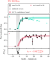 |
Fig. 2. Example of the time-of-explosion determination. We fitted an inverse exponential model (Eq. (8)) to the observed flux curves (black error bars), modelling the available bands (here g and r) jointly with a shared explosion time t0. The coloured bands (cyan for g, red for r) show the 95% confidence regions of the fits. The bottom panel displays the t0 posterior along with the inferred value relative to the first detection and its uncertainty. Finally, the inflated flux errors, including the additional fitted uncertainty σadd, are shown in grey. Here, the reported g-band uncertainties accurately capture the scatter around the model, resulting in minimal error inflation. In contrast, the r-band errors show noticeable inflation, with σadd around 0.06 mag. |
Time-of-explosion fit data and results.
Our methodology closely follows Csörnyei et al. (2023a,b) but with two key differences. We reformulated the prior for the exponential time scale te in terms of the rise time as discussed earlier and handled non-detections differently. While Csörnyei et al. (2023a,b) treated all non-detections as upper limits, with the model flux constrained to not exceed these limits, we used the actual flux measurements with their associated uncertainties, just like detections for the ePESSTO+ sample. This approach improves constraints on t0 by utilising all available information whereas the upper limits ignore the actual measured flux. For the literature sample, we continued using the old method for non-detections because we did not have the necessary flux values available.
4.2. Light curve interpolation
We used Gaussian processes (GPs; e.g. Rasmussen & Williams 2006) to interpolate the photometry to the epochs of spectral observations, similar to Inserra et al. (2018), Yao et al. (2020), Kangas et al. (2022), Csörnyei et al. (2023a,b).
We adopted a squared-exponential kernel to describe the smooth SN light curve and a white kernel to allow for additional uncertainties in the photometry compared to the reported values. We modelled the mean of our GPs with a constant function.
The GP regression was done with the Python package george12 (Ambikasaran et al. 2015). To avoid overfitting and improve uncertainty estimates, we marginalised over the values of the GP hyperparameters instead of optimising them with the more commonly used maximum likelihood method.
We sampled the hyperparameters with nestle, which we also used in the time-of-explosion fit (see Sect. 4.1). Our prior choice was guided by the Stan User’s Guide13: we used an inverse-gamma distribution for the length scale and a half-normal distribution for the standard deviation of the squared-exponential kernel.
The inverse-gamma prior suppresses small and large length scales where the marginal likelihood function becomes flat. We set its parameters so that only 1% of the prior probability is assigned to length scales below 10 or above 100 days.
The half-normal prior for the marginal standard deviation was centred at zero with a scale parameter σ = 1.5 mag. This assigns sufficient probability to small values such that the GP contribution can go to zero, for example, for a nearly flat R-band plateau light curve. At the same time it extends to large enough values to describe even the most steeply declining B-band light curves.
A standard log-uniform distribution for the white-kernel standard deviation completed our hyperparameter priors. The final parameter was the value of our constant mean function, which had a uniform prior.
We excluded the rise and fall from the plateau from the fit whenever possible14 because they bias the GP length scales to small values, making the fits too flexible during the plateau phase.
Finally, we drew a large number of samples (∼100 000) from the marginalised predictive probability distribution to obtain the photometry at the spectral epochs. Figure 3 shows an example of the interpolated light curves. Plots for the remaining SNe are in Appendix C.
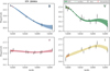 |
Fig. 3. Example of the GP interpolation of the photometry. We plot the observed magnitudes and their uncertainties in black; the interpolated values at the spectral epochs are shown in red. The coloured bands, finally, indicate the 68% confidence interval of the interpolated light curve and the dashed line the median. |
The interpolated photometry is not Gaussian: it is a Gaussian mixture. However, since deviations from Gaussianity are small in our sample, we approximated the distributions as Gaussian to simplify the subsequent analysis.
We list the mean and standard deviation of the interpolated magnitudes in Table A.1. The listed uncertainties are typically much smaller than those of the individual data points, despite the error inflation from the white kernel. This is because the GP assumes a smooth light curve, as encoded by the length scale, allowing us to average across multiple data points.
4.3. Spectral flux calibration
Our spectroscopic observations are not spectrophotometric due to the limitations imposed by the slit width and seeing conditions. However, for our radiative transfer models to yield accurate parameter values – particularly extinction and temperature – the spectra must have a reliable relative flux calibration. Therefore, we corrected our spectra using the photometric measurements interpolated to the epoch ofobservation.
We began by performing synthetic photometry on the observed spectra using the passbands described in Sect. 3.3. We then used the interpolated magnitudes from the previous section to calculate the ratios of the photometric and spectroscopic flux in the different passbands. Plotting the ratios against the effective wavelength reveals any wavelength-dependent trends in the flux calibration.
We fitted these trends with a parametric model, which we later applied to the observed spectra to correct them. However, the small number of passbands cannot constrain complex wavelength dependencies, so we used a linear model.
As for the GP hyperparameter estimation, we sampled the parameters with nestle. In addition to the slope and intercept of the linear model, we included a parameter that allows for additional uncertainties in the flux ratios. These uncertainties can arise from mixing different photometric systems, non-linear trends in the flux calibration, or underestimated uncertainties in the interpolated magnitudes. The additional uncertainty was added in quadrature to the existing values.
Because this additional uncertainty is often not well constrained by the data – due to the small number of passbands – we used a more informative prior than the standard log-uniform one used in the time-of-explosion fit (Sect. 4.1) and light curve interpolation (Sect. 4.2). We adopted a half-normal distribution with mean zero and a σ parameter15 of 0.03 mag. While the log-uniform prior is scale-invariant, the new prior is not, allowing it to better reflect the expected size of the neglected uncertainties, such as photometric system mismatches.
Fig. 4 shows an example of our linear fit to the flux ratios16. The plot illustrates that there is a wide range of possible flux calibration corrections that we can apply to the observations. We stored 100 randomly selected corrections, which allowed us to propagate the flux calibration uncertainties into the θ/vph values in Sect. 5.
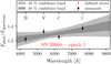 |
Fig. 4. Example of the linear flux calibration procedure. The plot shows the measured ratios of the photometric and spectroscopic flux Fphot/Fspectrum for the first epoch of SN 2006it as a function of wavelength in black. We performed a Bayesian fit of the ratios (see Sect. 4.3) to identify all possible linear flux calibration corrections. Of the possible curves 68% fall within the dark grey contour and 95% within the light grey contour. Although the underlying curves are straight, the contours naturally exhibit curvature. An important part of the fit is inflating the measured errors if necessary, accounting for additional unquantified uncertainties, such as the mixing of different photometric systems or underestimated uncertainties in the interpolated magnitudes. In the plot, the inflated errors are highlighted in red. In this specific example, the errors are substantially inflated because the data points deviate significantly from a linear trend within the measurement uncertainties. |
4.4. Spectral fits
After flux calibration, we fitted the calibrated spectra with radiative transfer models to estimate the photospheric velocities and specific fluxes at the photosphere fλem, ph needed for calculating θ/vph (see Eq. (4)). The radiative transfer models at the heart of this process were calculated with a custom version of the Monte Carlo code TARDIS (Kerzendorf & Sim 2014; Kerzendorf et al. 2023) that has been modified for use in SNe II as described in Vogl et al. (2019). The additional functionality of this version is currently being implemented in the main branch of TARDIS.
In the transport, we treated the ejecta as spherically symmetric and homologously expanding as in the EPM. We used simple input models, which are described by only a handful of parameters, so that we could explore the parameter space and find the best-fitting model. The key simplifications were a power-law density profile and uniform composition. Both choices greatly reduce the number of parameters and are well motivated for modelling SNe II in the photospheric phase (see the discussion in Dessart & Hillier 2006; Dessart et al. 2008; Vogl et al. 2020).
Exploring the parameter space automatically remains challenging, however, due to the computational cost of the radiative transfer simulations, which take around a day (∼105 s) per spectrum. To address this, we replaced our radiative transfer code with an emulator, drastically reducing the time to generate a spectrum to about 10−2 s – a difference of seven orders of magnitude. The emulator, which is trained on a large grid of TARDIS simulations (see Vogl et al. 2020), predicts the output of TARDIS with typically sub-percent accuracy. The models used for the training cover a wide range of photospheric temperatures Tph, velocities vph, metallicities Z, power-law indices for the density profile n, and values for the time since explosion texp. Csörnyei et al. (2023a) describe the most up-to-date models and the parameter space they cover (see their Table 2).
The strategy for finding the best-fitting model was similar to Vogl et al. (2020), Vasylyev et al. (2022, 2023), and Csörnyei et al. (2023a,b): we performed maximum likelihood estimation with a Gaussian likelihood. To do this, we used a simple diagonal covariance matrix that gives all parts of the spectrum equal weight. This choice provides a reasonable guess for the best fit but it does not yield realistic parameter uncertainties in a full Bayesian analysis. For the latter, we need a covariance matrix that summarises all sources of uncorrelated and correlated uncertainties. This includes, most importantly, the effect of approximations in our TARDIS models, which result in complicated correlated fit residuals even for noise-free data. If the covariance matrix does not account for these residuals, the parameter uncertainties will be significantly underestimated (see Czekala et al. 2015).
Given the unresolved challenge of incorporating these residuals into SN fitting, we limited our analysis to the described maximum likelihood estimation. In Sect. 6, we present a rough estimate of the impact of SN parameter uncertainties (and other unaccounted-for uncertainties) on distances from the dispersion in H0 between epochs and between objects.
Since the host extinction is unknown, we fitted for the SN parameters on a fine grid of host colour excess values E(B − V)host. This allowed us, as shown in Sect. 5, to determine a consistent E(B − V)host from all spectra of an object and estimate the contribution of the extinction to uncertainties in θ/vph. In the fits, we corrected the observed spectra for Milky Wayextinction (Table 1) and reddened the emulated spectra with the host extinction using a Fitzpatrick et al. (2019) extinction law with a total-to-selective extinction ratio RV = 3.117.
We calculated a maximum-likelihood θ/vph estimate for each E(B − V)host value, using the respective best-fit results for vph and the reddened emulated flux at the photosphere. For this, we recast Eq. (4) in terms of magnitudes (as described in Vogl et al. 2019) and used the interpolated magnitudes from Sect. 4.2 corrected for Milky Way extinction as the observed flux. We used all available passbands to constrain θ.
A close examination of Eq. (4) shows that K-corrections (e.g. Hogg et al. 2002) are unnecessary for the observed flux because the relevant transformations are instead applied to the model flux at the photosphere.
4.5. Flow corrections
To accurately measure H0, we must correct for the peculiar velocities of SN host galaxies using a cosmic flow model, as discussed in Sect. 2.2. Peculiar velocities can reach 300 km s−1 or more (see e.g. Léget et al. 2018), which can easily introduce a 10% error in the cosmological redshift and subsequently H0 for our lowest redshift objects (with cz ∼ 3000 km s−1). Due to this high error risk, these corrections are important, and their success in reducing Hubble diagram residuals (see e.g. Peterson et al. 2022) has led to their widespread adoption in recent H0 measurements (e.g. Pesce et al. 2020; de Jaeger et al. 2022; Riess et al. 2022).
We followed the approach used in the Pantheon+ analysis by adopting the 2M++/SDSS model from Carr et al. (2022). This model is based on the velocity field of Carrick et al. (2015) with updated values for the velocity scale parameter β and the external velocity vext from Said et al. (2020). We evaluated the model using the publicly available code18. The resulting peculiar velocities are listed in Table 1.
The Pantheon+ analysis suggests that we could further minimise the impact of peculiar velocities by assigning galaxies to groups and performing flow corrections on the groups (see Peterson et al. 2022). We investigated this possibility using their preferred group catalogue from Tully (2015). However, only three of our SNe (SN 2006it, SN 2010id, and SN 2020cvy) are in groups from this catalogue. These groups are small, with a maximum of three members, implying that the small-scale virial motions that could be averaged out are minimal. In fact, the group redshifts deviate from the host galaxy redshifts by less than 70 km s−1. Given this small difference, we refrained from using group assignments for simplicity. We examine the impact of this decision and of our choice of cosmic-flow model in Sect. 7.1.5.
5. Extinction and θ/vph determination
In Sect. 4.4, we described how to determine θ/vph for a given flux-calibrated spectrum and extinction. However, in practice, both flux calibration and extinction are subject to uncertainties, which must be accounted for when constraining θ/vph. The two uncertainties are deeply interconnected because the process of spectral fitting derives extinction from the observed slope of the spectrum.
While the SN parameters, including the photospheric temperature, can be inferred from spectral features without considering the slope, the difference between the predicted and observed slopes constrains the extinction. Since the observed slope depends on the flux calibration, uncertainties in the calibration directly affect the inferred extinction.
For example, a 20% change in flux calibration from the blue to the red end of the spectrum (3800–9000 Å) impacts the slope similarly to a differential extinction with E(B − V) = 0.05. Our flux calibration uncertainties can reach this magnitude, making them an important source of uncertainty in the extinctiondetermination19.
The spectral fits are the second key source of uncertainty. Even with a perfectly flux-calibrated, noise-free spectrum, a range of E(B − V) values can yield reasonable fits due to imperfections in the spectral models. Determining the exact size of this range is challenging because defining a “reasonable fit” statistically is difficult (see Sect. 4.4).
Based on their expertise in spectroscopy, Dessart & Hillier (2006) estimated that E(B − V) can vary by up to ±0.05 before the fits become unreasonable. This range of acceptable values is comparable to the uncertainties from flux calibration.
To determine θ/vph given uncertain extinction, we must account for both sources of uncertainty. By assigning reasonable uncertainties to the E(B − V) estimates from individual epochs, we can then combine them into a more precise joint constraint. Prior knowledge about the distribution of extinction values can further refine this estimate.
We explain the prior knowledge used in Sect. 5.1 and the combination of the constraints and determination of θ/vph in Sect. 5.2.
5.1. Extinction prior
Since E(B − V) cannot be negative, we must impose a non-negative prior. A simple approach is to use a positive flat prior, but this can bias the extinction towards higher values (see e.g. Jha et al. 2007). This bias occurs because measurements that scatter downwards into negative E(B − V) values are pushed up to zero by the prior, while upwards scatter remains unaffected, leading to an asymmetry.
If the distribution of SN host extinction were truly uniform from zero to infinity, values near zero would be extremely unlikely, making the bias negligible. However, in reality, extinction values close to zero are much more common than large ones. Therefore, using a prior that reflects this reality helps reduce bias by exerting a compensating pull on values that scatter upwards.
An example of such a prior was provided by Hatano et al. (1998), who used a simple model of the dust and SN distribution in randomly oriented galaxies to derive the extinction distribution for core-collapse SNe, which is widely used in the literature (e.g. Bazin et al. 2009; Goldstein et al. 2019; Vincenzi et al. 2023). Following Taylor et al. (2014), we approximated this distribution as exponential with a mean AV of 0.5.
5.2. Method
To combine our prior knowledge of E(B − V) with the constraints from the individual epochs and determine θ/vph, we propose the approach visualised in Fig. 5, which we explain step by step. The steps are numbered consistently in the text and the figure for easy reference.
The figure is based on a hypothetical supernova observed at two epochs, but the principle generalises to any number of epochs. All data and results shown are purely illustrative. We use colour coding to distinguish between the epochs: red for epoch 1 and blue for epoch 2.
We divide the explanation of the method into two parts: first, the determination of E(B − V), and second, the determination of θ/vph.
5.2.1. Determination of E(B − V)
-
Generating viable flux-calibrated spectra: To represent the uncertainty in the flux calibration, we generated sets of possible flux-calibrated spectra for each epoch. We randomly selected 100 linear flux calibration solutions from the posterior of the photometric to spectroscopic flux ratio fits (Sect. 4.3). These flux solutions were multiplied with the original SN spectrum to obtain 100 calibrated spectra per epoch.
-
Performing spectral fits: We performed maximum likelihood spectral fits on the created flux-calibrated spectra for a fine grid of host E(B − V) values (see Sect. 4.4). For each spectrum and each point of the E(B − V) grid, we obtained the best-fit values for the SN parameters, plus θ/vph. To account for flux calibration uncertainties that can make spectra appear artificially bluer, we extended the E(B − V) grid to include negative values, even though negative extinction is unphysical. This allowed us to fit these spectra and, by applying the extinction prior to exclude negative values, effectively filter out flux calibration solutions that are too blue (see step 4). For simplicity, Fig. 5 displays only a single fit per calibrated spectrum (shown in grey), rather than the full grid of fits for different E(B − V) values.
-
Deriving individual E(B − V) constraints: We derived constraints on E(B − V) for the individual epochs from the spectral fits. We started by identifying the best-fitting E(B − V) in the grid for each of the calibrated spectra as measured by χ2, which yielded a distribution of possible E(B − V) values for each epoch. This distribution captures the uncertainties in the extinction arising from the flux calibration. To account for uncertainties from the spectral fits, we considered E(B − V) values within ±0.05 of the best-fit value, as suggested by Dessart & Hillier (2006). We assumed all fits within this range to be equally likely. For each possible flux-calibrated spectrum, we represented the E(B − V) estimates with a uniform distribution over this range. By summing these uniform distributions from all flux calibrations, we obtained the final E(B − V) estimate for each epoch. This method is essentially a kernel density estimation (KDE) using a tophat kernel with a bandwidth of 0.05 (see e.g. Bishop & Nasrabadi 2007). We discuss the impact of the bandwidth choice in Sect. 5.3. In the figure, plus symbols indicate the distribution of best-fitting E(B − V) values for each possible flux calibration; the resulting KDEs are shown by solid lines, with epoch 1 in red and epoch 2 in blue. The extinction prior (Sect. 5.1) is shown in black, positioned between our estimates derived from the spectral fits.
-
Deriving a joint E(B − V) constraint: To derive the combined E(B − V) constraint, we treated the estimates from the individual epochs as independent and multiplied them with the prior. However, directly multiplying the top-hat KDEs with the continuous exponential prior creates an artificial sawtooth pattern. To prevent this, we approximated the prior as piecewise constant within the regions where the product of the two top-hat KDEs is constant. This ensured a well-behaved joint posterior, shown in teal in the figure.
5.2.2. Determination of θ/vph
Having arrived at a final E(B − V) distribution, we now explain how this translates to the θ/vph values we are ultimately interested in:
-
Drawing E(B − V) posterior samples: The first step was to sample a large number of E(B − V) values (10 000) from the posterior to approximate the distribution. In the diagram, we represent this random process with dice rolls, yielding two example values: E(B − V)⚂ and E(B − V)⊡.
-
Identifying consistent flux calibrations for E(B − V) samples: Next, we connected the E(B − V) samples back to the spectral fits, which provide the θ/vph constraints. We started by identifying the flux calibrations that are consistent with each E(B − V) sample. As established earlier, for each flux calibration we treated all E(B − V) values and associated spectral fits within ±0.05 of the best fit as valid and equally likely. Reversing this logic, all flux calibrations within this range of an E(B − V) sample were considered consistent with it. We illustrate this process in the figure using our two exemplary samples E(B − V)⚂ and E(B − V)⊡. For each sample (indicated by the dashed line), we show the distribution of best-fitting E(B − V) values for the different flux calibrations from step 3. The consistent calibrations fall within ±0.05 of the sample and are shown in colour; the inconsistent calibrations are greyed out.
-
Selecting consistent flux calibrations for E(B − V) samples: We randomly selected one consistent flux calibration for each E(B − V) sample and epoch for the determination of θ/vph. This random selection is represented in Fig. 5 by two dice rolls for each example extinction value, E(B − V)⚂ and E(B − V)⊡.
-
Determining θ/vph for the selected flux calibrations and extinction: For each E(B − V) sample (e.g. E(B − V)⚂), we computed the corresponding θ/vph values using its selected flux calibration. Each flux calibration has its own grid of maximum-likelihood spectral fits, providing θ/vph values for a grid of E(B − V) values. We interpolated these θ/vph values to match each E(B − V) sample. By repeating this process for all 10 000 samples, we generated a distribution of θ/vph that incorporates uncertainties from both extinction and flux calibration. This approach also captures correlations between epochs, as for each θ/vph pair, the epochs share the same extinction, pushing them on average in a similar direction with respect to the mean20.
-
Including additional θ/vph uncertainties: Besides flux calibration, other observational uncertainties affect θ/vph. For this proof-of-principle paper, we focused on only two major sources: uncertainties in the observed flux21 affecting the θ calculation (see Eq. (4)) and errors in the heliocentric redshift correction due to host galaxy rotation. We quantified the flux uncertainties through linear error propagation based on the interpolated magnitude uncertainties from Table A.1. Given that the magnitude uncertainties are small and multiple bandpasses are combined, the uncertainties in θ are generally less than ∼1.5%. For redshift correction errors, we assumed an average uncertainty of 150 km s−1, as the correction typically uses the redshift of the galaxy centre, while the SN is located in a rotating spiral arm, following de Jaeger et al. (2020b). This translates to an uncertainty in photospheric velocities of a similar size22. For our sample, spanning photospheric velocities between 5000 km s−1 and 10 000 km s−1, this contributes ∼1.5–3% to the θ/vph uncertainties. To propagate these uncertainties into our samples, we applied random offsets to the θ values based on the observational flux uncertainties and to vph based on the heliocentric redshift uncertainty.
-
Determining mean and covariance of the θ/vph samples: We then determined the mean and covariance CSNX, meas of the θ/vph samples of the different epochs, which we use in the EPM regressions (Sect. 6) to constrain the SN distances.
5.3. Results
We show an example of the extinction determination and the involved spectral fits in Fig. 6, while plots for the remaining objects can be found in Appendix E.
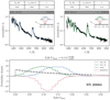 |
Fig. 6. Example spectral fits. We show the spectral fits for SN 2006it at two epochs (Oct. 10 and Oct. 13), analogous to the hypothetical SN used in Fig. 5. The bottom panel displays the E(B − V) constraints from spectral fits of possible flux calibration solutions, with epoch 1 in blue and epoch 2 in green. The constraints from both epochs align well within the uncertainties. The dashed black line represents the exponential approximation of the Hatano et al. (1998) extinction prior, with dots indicating evaluation points for multiplication with the individual epoch constraints. We plot the final E(B − V) posterior (red) in the negative probability density direction for visual separation. The upper part of the figure visualises the spectral fits contributing to the E(B − V) and subsequently θ/vph determinations. While fits of many different flux-calibrated spectra and E(B − V) values contribute, we show only one representative fit per epoch for simplicity. To select this fit, we follow a two-step process. First, we choose one of the flux calibration solutions whose best-fit E(B − V) is closest to the median of the posterior. Next, within this flux calibration solution, we analogously identify the fit from the E(B − V) grid that is nearest to the median of the posterior. The normalised observed specific flux fλ of this choice appears in black, with the corresponding maximum-likelihood fits in blue (epoch 1) and green (epoch 2). The key physical parameters for the selected fits are listed on the top. Small insets in each panel mirror the bottom half of the figure, visualising the E(B − V) constraints with the other epoch greyed out. The dashed line in the inset marks the median E(B − V) value, which is used in the plotted fits. |
The precision of the host E(B − V) determinations varies significantly, ranging from 0.015 to 0.08. This variation reflects differences in flux calibration uncertainties and the number of available epochs. Consequently, the quantified uncertainties in θ/vph also span a wide range, from roughly 3–13%, with a median of around 4%.
Our results are somewhat influenced by the bandwidth choice for the KDE in the E(B − V) determination. To assess this, we increased the bandwidth by 50%, from 0.05 to 0.075. This change moderately increased E(B − V) uncertainties by a median of 23%, but only slightly increased θ/vph uncertainties by 4%. The mean θ/vph values changed only slightly, with a median decrease of 0.4%. Thus, while the bandwidth affects the results, the overall sensitivity is low.
While our quantified uncertainties account for significant sources like extinction, interpolated magnitudes, and heliocentric redshift corrections, they are not exhaustive. We do not consider, for example, uncertainties from model imperfections or the total-to-selective extinction ratio on the modelling side. Observationally, non-linear trends in the flux calibration or wavelength calibration issues are also not included. In the next section, we attempt to statistically constrain the combined uncertainties from these sources together with the Hubble constant.
6. Hubble constant
The measured θ/vph values constrain the luminosity distances of our SNe, thereby constraining H0 as explained in Sect. 2. Traditionally, this involves two steps: fitting the time evolution of θ/vph for each SN individually and analysing the resulting Hubble diagram for H0. However, we devised a different strategy in which we directly fit for H0 using all SNe.
Our motivation for this departure lies in the need to statistically capture the remaining scatter in θ/vph not explained by the quantified uncertainties, akin to the intrinsic dispersion term σint in SN Ia cosmology (see e.g. Astier et al. 2006; Scolnic et al. 2018; Dhawan et al. 2018). Since σint is a global parameter, we adopted a collective approach by performing all EPM regressions simultaneously.
Termed Bayesian ensemble EPM, our approach accounts for both the constraints from the scatter of θ/vph within each SN and the scatter between SNe in the Hubble diagram. We explain the method in Sect. 6.1, validate it with simulated data in Sect. 6.2, and then apply it to our real data in Sect. 6.3.
6.1. Bayesian ensemble EPM
In contrast to the classical EPM regression, we did not use independent values for the SN luminosity distances DL, SNX in the fit. Instead, we proposed a shared value for H0 and simultaneously proposed values for the true SN cosmological redshifts zcosmo, SNX. Together, these inputs, along with the cosmological model described by Eq. (6), generated a trial set of interconnected DL, SNX, whose viability we evaluated simultaneously.
To evaluate this viability, we first calculated the predicted θ/vphpred values from the proposed distances and explosion times t0, SNX using Eq. (5). We then evaluated the likelihood by comparing the predicted and measured θ/vph values for all SNe. The flowchart in Fig. 7 summarises the procedure, including the equations used.
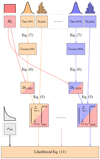 |
Fig. 7. Flowchart of the iterative procedure for parameter estimation in the Bayesian ensemble EPM fit. At each step, we sample a new set of parameters, including the Hubble constant H0, unexplained dispersion σint, and the peculiar velocity vpec and time of explosion t0 for each SN, from the priors. The priors are visually indicated above each parameter. From the parameters, we then calculate true cosmological redshifts zcosmo and luminosity distances DL, ending with the computation of the proposed θ/vphpred vectors using the referenced equations. The process concludes with the comparison of the proposed and measured θ/vph vectors, evaluating the likelihood for the proposed σint. This cycle repeats for each new set of parameters, slowly building up the posterior distribution. |
As in the regular EPM regression, we used a Gaussian likelihood ℒ for each SN:
 (9)
(9)
Here, CSNX is the covariance matrix and
 (10)
(10)
are the θ/vph residuals for the NX epochs of SN X.
The distinguishing feature of the ensemble EPM is the combination of the individual SN likelihoods into a joint likelihood
 (11)
(11)
This approach enables us to quantify the unexplained scatter in θ/vph by combining constraints from within each SN and between SNe – our main motivation for the method.
To achieve this, we modelled the scatter as uncorrelated between epochs and as a consistent fractional uncertainty for θ/vph, which is constant across all SNe. The covariance matrix is thus
![Mathematical equation: $$ \begin{aligned} C_\mathrm{SN X} = C_\mathrm{SN X, meas} + \left[ \sigma _\mathrm{int} \, \mathrm{diag } \begin{pmatrix}\frac{\theta }{v_\mathrm{ph} }_1\\ \vdots \\ \frac{\theta }{v_\mathrm{ph} }_{N_X}\end{pmatrix}_\mathrm{SN X} ^{\mathrm{pred, H_0 = 70} } \right]^2, \end{aligned} $$](/articles/aa/full_html/2025/10/aa52910-24/aa52910-24-eq27.gif) (12)
(12)
where CSNX, meas is the measured covariance matrix (see Sect. 5 and Fig. 5) and σint the additional fractional uncertainty. To avoid biases, we used the predicted θ/vph values in the uncertainty calculation rather than the measured ones23.
We made one additional adjustment to further prevent biases: we employed a fixed H0 of 70 km s−1 Mpc−1 in computing the fractional uncertainties. This strategy decouples the fitted H0 from the complexity penalty, which penalises models that can accommodate a wider range of observed data24. We chose 70 km s−1 Mpc−1 for convenience, given its proximity to typical measured values. The specific choice is unimportant since σint is rescaled to match the measured H0 at the end (Sect. 6.3).
Our assumptions in modelling the unexplained θ/vph scatter are not entirely accurate. Particularly, the errors resulting from the limitations within the spectral models likely vary across different epochs and SNe due to the diverse physical conditions in the spectrum-formation regions. Our current data, however, do not provide sufficient statistical power to detect more complex trends in the uncertainties.
With the likelihood and uncertainty model established, the next step was to define the prior distributions for our parameters: we adopted a flat prior for H0 and a log-uniform distribution for the unexplained scatter σint (e.g. Rubin et al. 2015; de Jaeger et al. 2022). The priors for explosion times t0, SNX were based on the posterior distributions from the early light curve fits (see Sect. 4.1). Finally, the priors for the peculiar velocities, used to compute the cosmological redshifts of the SNe, followed normal distributions with means derived from the flow model (see Sect. 4.5). Their standard deviations included a peculiar velocity uncertainty of 250 km s−1 similar to the Pantheon+ analysis (Brout et al. 2022; Peterson et al. 2022), and the redshift measurement errors added in quadrature.
The redshift measurement errors were taken from NED except for SN 2021gvv, for which we measured the redshift ourselves from narrow host galaxy emission lines. The median redshift measurement error from NED is 5 km s−1, and the maximum is about 90 km s−1, both of which are negligible compared to the peculiar velocity uncertainty. However, for SN 2021gvv, from the dispersion of the narrow host galaxy emission line measurements, we estimated an error of around 200 km s−1, which is comparable to the peculiar velocity uncertainties.
6.2. Validation with simulated data
We checked that we can retrieve H0 without biases and with meaningful uncertainties by fitting simulated datasets with a known H0 of 70 km s−1 Mpc−1. The simulated data closely match our real observations; we did not explore whether the method generalises to new datasets with, for example, a different redshift distribution.
The first step in the mock data generation was to sample true values for the cosmological redshifts and explosion times from the established priors. From these and the selected H0 (70 km s−1 Mpc−1), we then calculated true values for θ/vph at the observed spectral epochs. The procedure is identical to the computation of the proposed θ/vph values in the Bayesian ensemble EPM fit.
In the final step, we converted the true θ/vph values to observed ones by applying random offsets drawn from the covariance matrices CSNX. Here, the measured covariance matrices CSNX, meas were the same as for the real data and we assumed two plausible values (5% and 10%) for the additional unexplained scatter σint.
For each σint value, we generated 100 realisations with different true redshifts, explosion times, and θ/vph, and fitted them using our method. These realisations differ from our actual data only in their mean θ/vph values.
Table 3 summarises the fit results. We show the mean inferred values for H0 and σint along with the uncertainty on the mean demonstrating that we can retrieve these key parameters without discernible biases. The accurate inference of the unknown additional uncertainty σint is a promising indication that the method provides meaningful H0 uncertainties. To confirm this, we calculated the reduced chi-square of the H0 values around the true value χH0, red2, yielding a result consistent with unity, as expected for accurate uncertainties.
Validation of the Bayesian ensemble EPM with simulateddata.
6.3. Results
Building on the successful fits of our simulated data, we applied our method to analyse the actual dataset. Utilising the nestle algorithm as in Sect. 4.2 to 4.1, we sampled the parameters to derive a 22-dimensional posterior distribution (H0, σint, t0, SN1, …, t0, SN10, vpec, SN1, ..., vpec, SN10). A two-dimensional projection of the posterior, highlighting the key parameters H0 and σint, is illustrated in Fig. 8 using the corner Python package (Foreman-Mackey 2016). Our fit yields a Hubble constant of 74.9 ± 1.9 km s−1 Mpc−1.
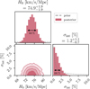 |
Fig. 8. Posterior of the Bayesian ensemble EPM fit (marginalised over the times of explosion and peculiar velocities of the SNe). The plot shows the 68% confidence intervals for the one-dimensional distributions. The two dimensional projection displays the 39.3%,67.5%,86.5%,95.6% confidence regions (corresponding to the 1σ, 1.5σ, 2σ, 2.5σ levels of a two-dimensional Gaussian distribution, as described in the corner Python package documentation) (https://corner.readthedocs.io/en/latest/pages/sigmas/). The prior distributions for the one-dimensional marginalised distributions are shown as grey dashed lines. |
A comprehensive comparison of our H0 with estimates from other methods, alongside a discussion on its precision, is provided in Sect. 7.2. We address potential systematic uncertainties that could impact our findings in Sect. 7.1.
We determine σint to be  %, which has been obtained by rescaling the fit result from the fiducial H0 value of 70 km s−1 Mpc−1 to the median measured value of 74.9 km s−1 Mpc−1 through a multiplication by the factor 70/74.9 (see Eqs. (5), (6), and (12)). Our measured σint is significantly lower than the median quantified θ/vph error of approximately 4% (see Sect. 5). As a result, the combined median θ/vph uncertainty remains essentially the same as the quantified uncertainty, around 4%, which is less than half of the heuristic estimate of 10% proposed in Dessart & Hillier (2006) and employed in our previous studies (Vogl et al. 2020; Csörnyei et al. 2023a,b).
Although the posterior distribution of σint includes higher values (up to a few percent), values large enough (≳9%) to push the combined uncertainty beyond the Dessart & Hillier (2006) threshold are essentially ruled out, comprising less than 0.02% of the posterior. However, this conclusion depends on the accurate quantification of the explosion time and peculiar velocity uncertainties. Should these uncertainties have been overestimated, σint might be higher than calculated.
The precision of our H0 measurement, 1.9 km s−1 Mpc−1, slightly surpasses that achieved in the simulated data fits (see Sect. 6.2), where a median precision of 2.2 km s−1 Mpc−1 was obtained with σint = 5%. This improvement is due to the lower intrinsic scatter, σint= %, in our real data.
We present a visualisation of the fit in Fig. 9. To reflect the internal dynamics of the fit, the most precise method would be to display ten separate EPM regression diagrams, each tracking the temporal evolution of θ/vph for an individual SN (as in the schematic example in Fig. 1).
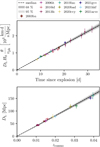 |
Fig. 9. Visualisation of the Bayesian ensemble EPM fit. The upper panel presents the combined EPM regressions for all SNe, with θ/vph values scaled by the Hubble-free luminosity distance DL(zcosmo)H0, placing them on a uniform absolute scale. Each spectrum contributes one measurement to this plot, with the median of the fit indicated by a dashed line. The 68% and 95% confidence intervals are shown in light and dark grey, respectively. Each SN is colour-coded for clarity. The error bars include the inferred additional uncertainty σint. In the bottom panel, we complement this visualisation with a plot similar to a classical Hubble diagram, where DL values, derived by solving Eq. (5), are plotted against their redshifts. Unlike traditional Hubble diagrams, each point represents one epoch of an SN, with all spectra for a given SN appearing at the same redshift. Special care is needed when interpreting the error bars. In the EPM-like visualisation, the y-errors include both θ/vph and peculiar velocity uncertainties, whereas in the Hubble-diagram-like visualisation, they include both θ/vph and time of explosion uncertainties. The time of explosion and peculiar velocity uncertainties are completely correlated for all epochs of an SN, introducing correlations in the y-error bars that cannot be captured in this figure. The situation is even worse for the uncertainties in the x-direction, which are solely the time of explosion and peculiar velocity uncertainties, and thus are 100% correlated. The data points are thus not independent, making it more difficult to assess aspects like the dispersion around the fit. It is important to remember, however, that we do not use the plotted data points for the fit; instead, we use the θ/vph values directly. |
However, this approach does not clearly demonstrate the interconnection of SNe through the shared H0 and complicates the assessment of sample properties, such as the dispersion around the fit or suspicious trends that could hint towards systematic errors. To address these issues, we combined all EPM regressions into a single plot, scaling the θ/vph values by the Hubble free luminosity distance DL(zcosmo)H0. This places them on a uniform absolute scale, where the slope of the fit corresponds directly to the Hubble constant.
In the bottom panel of Fig. 9, we complement the EPM regression-like plot with a visualisation similar to a classical Hubble diagram. To achieve this, we solved Eq. (5) for DL, using our prior knowledge of zcosmo and t0 for all epochs of all SNe, and plotted the resulting DL values against their redshifts. Unlike a traditional Hubble diagram, where each point represents a single SN, here each point represents an epoch of an SN.
Both visualisations indicate that the data closely follow the expected trends with minimal dispersion and no obvious systematic errors. For instance, any deviation from a linear trend in the EPM-like visualisation after the hydrogen recombination epoch (∼20 d) might suggest that neglecting time-dependent ionisation introduces errors in the distance calculations at these phases. While the current dataset does not allow for stringent constraints, future datasets will enable these plots to be powerful tools for identifying potential systematics in the method.
7. Discussion
In the previous section, we present our measurement of the Hubble constant H0. While the value of H0 is crucial, the accompanying uncertainty is equally important to understand the significance of the result. To contextualise our measurement, we first address systematic uncertainties not included in the statistical error in Sect. 7.1. Once these uncertainties are understood, we compare our results to other H0 estimates from the distance ladder, early universe measurements, and comparable one-step local methods in Sect. 7.2.
7.1. Sources of systematic uncertainties
7.1.1. Modelling limitations
Radiative transfer modelling is central to our measurement of H0; however, approximations in both the radiative transfer and parameterised SN models can introduce systematic errors in the inferred distances.
Potential errors stem from several key approximations. For example, in the radiative transfer, the lack of a full non-local thermodynamic equilibrium (NLTE) treatment for all species can affect the results. In the parameterised SN models, the assumption of a power-law density profile may not accurately reflect the true structure of SN ejecta.
These approximations influence our measurements in two ways: they can directly impact the luminosity for a given set of parameters, and they can alter the spectral appearance, leading to incorrect parameter inferences and subsequently biased luminosity estimates.
An example for the first mechanism is the assumption of a power-law density profile. By neglecting the flattening of density profiles towards the centre of SNe II, we might overestimate the density in the continuum-forming regions. This overestimation leads to less flux dilution and, consequently, an overestimate of the luminosity, while causing minimal changes to the spectral appearance.
An example for the second mechanism is the approximate treatment of excitation and ionisation for iron-group elements responsible for metal line blanketing. This simplification might cause us to systematically misestimate the photospheric temperature to match the observed strength of metal line blanketing.
Beyond these examples, other approximations could affect our results, such as assuming spherical symmetry, homologous expansion, and steady-state conditions for the radiation field and plasma state. While addressing all these factors in detail is beyond the scope of this paper, testing these sources of error is crucial for establishing a solid foundation for our method.
An important approach to assess these limitations is by comparing our models to more comprehensive simulations, either with more sophisticated input models featuring realistic ejecta structures or with more advanced radiative transfer physics – or both. The gold standard here is time-dependent NLTE CMFGEN models, based on hydrodynamical simulations of exploded stellar evolution models (e.g. Dessart & Hillier 2011; Hillier & Dessart 2019). These models are ideal for testing but not suited for spectral fitting because they are computationally intensive and their complex ejecta structures cannot be adequately described by a small set of parameters.
Although we have not conducted extensive tests with these advanced models yet, our code has been applied to some of the same problems as the older, steady-state version of CMFGEN, showing good agreement – specifically in the calculation of dilution factors and distance measurements for SN 1999em and SN 2005cs.
The temperature-binned dilution factors from Dessart & Hillier (2005) and Vogl et al. (2019) agree within a few percent, with maximum deviations of 8% after approximately accounting for differences in average photospheric densities between the model sets.
For SN 1999em, the distance estimates from Dessart & Hillier (2006) (11.5 ± 1.0 Mpc) and Vogl et al. (2020) (11.4 ± 1.0 Mpc) are in remarkable agreement. Both estimates also align well with the Cepheid distance of the host galaxy, 11.3 ± 0.5 Mpc (de Jaeger et al. 2020a).
For SN 2005cs, our best distance estimate is 7.3 ± 0.4 Mpc (Csörnyei et al. 2023b), which disagrees by almost 20% with the estimate from Dessart et al. (2008) of 8.9 ± 0.5 Mpc. This discrepancy can largely be explained by a difference of 1.6 d in the assumed explosion time: our study incorporates additional constraints from the early light curve, whereas Dessart et al. (2008) rely solely on the EPM regression. This time difference translates to approximately a 16% difference in distance at the median phase of the CMFGEN models (∼10 d), explaining most of the 20% deviation.
While these agreements are encouraging, they do not eliminate the need for more direct comparisons, especially with more complex time-dependent calculations.
Nevertheless, we can also assess the impact of modelling limitations empirically, as they do not affect every SN and epoch equally. For example, the approximate NLTE treatment of species other than hydrogen and helium likely becomes significant only after prominent metal lines develop. Similarly, neglecting time dependence in the ionisation balance becomes important once hydrogen recombination sets in (see e.g. Dessart et al. 2008).
If these approximations cause significant errors, we would expect to see variations in the inferred distances during the phases where these effects are important compared to when they are not – unless compensated by other errors. However, we do not observe strong evidence for such variations in the objects studied here (see Fig. 9) or in the sibling SN analysis by Csörnyei et al. (2023a).
Although larger sample studies are necessary for definitive answers, the low dispersion between objects and epochs in our study and in Csörnyei et al. (2023a) suggests that modelling limitations do not introduce substantial errors. Since most limitations are more significant at certain epochs and for certain objects, they would lead to some dispersion if they were a dominant error source.
In conclusion, while modelling limitations warrant further investigation, the evidence suggests that they are not overwhelmingly detrimental to our distance measurements. Continued efforts to test and refine our models – through comparisons with more sophisticated simulations and empirical studies – will enhance the reliability of our method.
7.1.2. Circumstellar material
Narrow emission lines in early-time spectra (e.g. Khazov et al. 2016; Bruch et al. 2021, 2023) and light curve modelling (e.g. Morozova et al. 2017) suggest that confined circumstellar material (CSM) is common around SNe II, although the mass-loss mechanism responsible remains debated (Fuller 2017; Fuller & Tsuna 2024). This topic has gained attention in recent years, sparked by early observations of events like SN 2013fs, which exhibited narrow emission lines for less than two days post-explosion (Yaron et al. 2017), and more extreme cases like SN 2023ixf, where narrow lines persisted for nearly ten days (e.g. Teja et al. 2023; Jacobson-Galán et al. 2023).
The first mechanism through which CSM could affect our measurements is a potential boost in luminosity due to ongoing interaction. If the ejecta-CSM interaction continues beyond the early explosion phases, it can produce additional luminosity currently not accounted for in the models, potentially leading to errors in the inferred luminosity.
For this effect to significantly impact our measurements, the interaction would need to persist during the epochs where our models are typically applied – more than ten days post-explosion. Given the confined nature of the CSM, this type of ongoing interaction may be unlikely at these phases. For example, Jacobson-Galán et al. (2024) suggested that SNe like SN 2013fs, with short-lived narrow lines, originate from compact CSM with radii smaller than around 5 × 1014 cm. In these cases, the CSM would likely be swept up by the ejecta within a few days, given typical ejecta velocities of around 10 000 km s−1. Additionally, Bruch et al. (2023) found no significant differences in the early light curves of SNe II with or without early narrow emission lines, suggesting that CSM interaction might not significantly impact the light curve in most cases, except in rare events where narrow lines persist beyond ten days.
The second mechanism by which CSM interaction could affect our measurements is through changes to the ejecta structure and kinematics, influencing the spectral appearance of the SN long after the interaction has ended (e.g. Hillier & Dessart 2019). Since these effects are not incorporated into our models, they can introduce biases in the inferred parameters and ultimately in the luminosity.
One example is the deceleration of the fastest-moving ejecta during the interaction, which leads to a deficiency of high-velocity material. To account for this in our power-law density models, we can only mimic the effect by steepening the gradient. However, this adjustment may overestimate the density in the continuum-forming layers, reducing flux dilution and slightly overestimating the luminosity.
While these mechanisms show how CSM interaction could introduce biases, its effect on the tailored EPM has not been extensively studied. Nevertheless, theoretical and empirical approaches offer promising ways to explore this further. On the theoretical side, fitting simulations that include CSM interaction, such as those by Hillier & Dessart (2019) and Dessart & Jacobson-Galán (2023), with our models could help quantify the errors introduced by ignoring this interaction.
Empirically, we could try to analyse larger SN samples to determine whether objects with CSM interaction exhibit systematically different distance estimates by studying SNe in the Hubble flow or sibling SNe in the same galaxy. One significant advantage is that CSM interaction often leaves clear spectral imprints, such as an Hα profile with a weak or absent absorption component (Hillier & Dessart 2019), which can persist for weeks post-explosion. These features allow us to identify and test objects affected by CSM interaction.
In our current sample, only SN 2013fs shows spectral signs of CSM interaction, and it does not significantly deviate from the rest. Based on this one object, we cannot draw strong conclusions about small systematic errors. However, since only one out of ten SNe in our sample shows evidence of CSM interaction, the overall impact on distance measurements in this study is likely small.
7.1.3. Total-to-selective extinction ratio
Systematic errors can also arise from the host galaxy extinction. We can estimate the colour excess through our spectral fits, as described in Sect. 5, by aligning the slopes of the model and observed spectra. However, our optical spectra do not strongly constrain the total-to-selective extinction ratio RV because the slopes of the reddened model spectra are relatively insensitive to RV for a given E(B − V); the slope in the B and V filters stays constant by definition. Differences in R and I only become noticeable for large changes in RV.
Consequently, we adopted a fixed RV of 3.1, typical of Milky Way dust. However, even in the Milky Way, RV varies slightly (σ(RV)≈0.2; Schlafly et al. 2016). Galaxies in the local universe exhibit a wider range of RV values (e.g. Salim et al. 2018), and similar diversity is found in SNe Ia (e.g. Johansson et al. 2021; Wojtak et al. 2023; Thorp et al. 2024). While the situation for SNe II is less studied, they likely also exhibit some variation in RV, introducing at least statistical uncertainty.
A systematic error could arise if the average RV for SNe II deviates from 3.1, similar to SNe Ia, where lower values around 2.5 are commonly reported (see e.g. Table A.1 of Thorp et al. 2024, summarising recent measurements). Although SNe Ia and II occur in different environments and may not share the same dust properties, the lower average RV in SNe Ia provides a useful benchmark for assessing the impact of RV.
The effect of RV is most easily demonstrated in the V-band, where the extinction equations are particularly simple. Specifically, the photospheric angular diameter θV depends on the extinction properties as follows:
 (13)
(13)
Assuming that the SN parameters and E(B − V) derived from the spectral fits remain unaffected by RV, which is reasonable given the weak sensitivity of the slope and shape of the dereddened model spectrum to RV, we can calculate θ for any new RV, relative to our reference value of 3.1:
 (14)
(14)
 (15)
(15)
Since the ratio in other bands will be similar, given the weak sensitivity of the slope and shape of the optical extinction curve to RV, we estimate that lowering RV to 2.5 results in roughly a 2% decrease in θ/vph for the median E(B − V)host of our sample (0.065). Because H0 is directly proportional to θ/vph, we expect this change to similarly decrease H0.
To verify our back-of-the-envelope calculation, we rescaled the θ/vph values for our spectral fits, including all flux calibration solutions and E(B − V) values. We then obtained updated values for the mean and covariance of the joint θ/vph distribution through the procedure in Sect. 5, and repeated the H0 fit as in Sect. 6, confirming the 2% decrease in H0. This 2% decrease is comparable to the statistical uncertainty of our measurement, demonstrating that extinction could be an important source of systematic uncertainty.
Given the potential impact, further study of the extinction properties in SNe II is crucial. This can be achieved either directly, through optical, UV, and infrared data, or indirectly by examining trends in Hubble residuals and distance discrepancies between SN II siblings as a function of extinction.
However, Salim et al. (2018) find that quiescent galaxies have an average RV of 2.61, while star-forming galaxies have an average RV of 3.15. This suggests that the lower RV observed in SNe Ia might result from their presence in both quiescent and star-forming galaxies. In contrast, SNe II almost exclusively occur in star-forming galaxies, making it likely that their average RV is closer to the Milky Way value of 3.1 used in our study. This would potentially reduce the impact of this systematic uncertainty on our measurements.
7.1.4. Photometric system
The calibration and characterisation of the photometric system represent another significant source of systematic errors, introducing correlated uncertainties across all SNe observed with the same instrument. These uncertainties fall into two maincategories:
-
Uncertainties in the calibration of photometric zero points (ZPs), directly affecting the observed magnitudes.
-
Uncertainties in the quantification of passbands, which are crucial for performing synthetic photometry that can be compared to observations.
These uncertainties impact our measurements through two avenues. First, in the direct calculation of θ (see Eq. (4)), which uses the observed magnitudes (fλ, obs) and synthetic model magnitudes (fλem, ph). Second, in the spectral recalibration, where observed photometric flux is compared to synthetic flux from observed spectra. Here, photometric uncertainties can systematically alter the colour of recalibrated spectra, which then propagates into the parameters inferred from spectral fits.
While ZP and passband uncertainties affect measurements through similar mechanisms, their statistical properties differ: ZP uncertainties influence all SNe (and epochs) observed with the same instrument uniformly. Passband uncertainties depend on the spectral slope and shape, leading to varying effects across SNe and epochs.
Relatively modern surveys, such as CfA3, tend to have small ZP uncertainties (∼0.01 mag), while older surveys can exhibit larger uncertainties, around 0.03 mag (see Table 2 of Rubin et al. 2025). Passband uncertainties are more complex, involving the full wavelength-dependent transmission function. To manage this complexity, they are typically approximated by wavelength shifts of the measured passband. Rubin et al. (2025) find that shifts smaller than 100 Å usually suffice to align observed and synthetic colour terms, though shifts exceeding 200 Å occasionally occur.
For the ePESSTO+ spectra, passband shifts of 100 Å change synthetic magnitudes on the order of 0.01 mag, similar to the estimated ZP uncertainty. However, since passband uncertainties are more statistical, they partially average out. Therefore, we focus primarily on ZP uncertainties when estimating the impact of the photometric system.
A typical ZP uncertainty of 0.01 mag would cause a 0.5% error in θ (and consequently H0) through avenue one if all SNe were observed in a single band with the same instrument. However, since our measurements span multiple bands and instruments, this small 0.5% error becomes even less significant.
In the second avenue (spectral recalibration), the effect is strongest for SNe observed in only two filters, as is the case for much of the ePESSTO+ sample. Here, a systematic error of 0.014 mag ( ) in the g − r colour could lead to a corresponding E(B − V) error of a similar magnitude25. This would result in a non-negligible systematic error in θ and H0 of around 2%, calculated using Eq. (13), comparable to the statistical uncertainty. The availability of i-band photometry for some ePESSTO+ objects helps mitigate this effect. Additionally, since the ePESSTO+ sample represents only 60% of our dataset, the impact is further reduced.
An additional systematic uncertainty specific to ZTF photometry arises from the so-called “pocket effect”, a nonlinear, signal-to-noise-dependent flux bias introduced by CCD waveform readout changes in November 2019 (Rigault et al. 2025; Ginolin et al. 2025). Except for SN 2019luo, all ePESSTO+ SNe in our sample are affected by this bias. Preliminary analyses by the ZTF collaboration indicate that the bias is colour-independent and of the order of 1% in the magnitude range of 15–19 (Ginolin et al. 2025), which covers most objects in our sample. Thus, its magnitude is comparable to typical ZP uncertainties. However, unlike ZP errors, it is nonlinear and may vary between objects based on signal-to-noise ratio. Its lack of dependence on colour means it does not affect extinction estimates from spectral recalibration but also implies no reduction from multi-band observations. Based on these properties, we estimate that the pocket effect introduces a systematic uncertainty in θ (and thus H0) on the order of 0.5% for the ePESSTO+ subsample, which is likely smaller than the corresponding classical ZP uncertainty.
In summary, photometric system uncertainties, particularly their impact on observed colours, can be significant sources of systematic error when most observations are from the same instrument. However, in our study, these uncertainties are likely subdominant to statistical errors, as we utilise data from multiple instruments and typically observe in more than threefilters.
7.1.5. Peculiar velocities
Our measurement of H0 depends on correcting the observed redshifts of SN host galaxies for their peculiar velocities. While these corrections are necessary, they are not uniquely defined, and different correction schemes vary in their predicted peculiar velocities. Our baseline cosmic flow correction modifies the redshifts, and consequently the inferred distances, by up to approximately 4%. Given this sensitivity, variations among different flow correction methods have the potential to systematically affect our analysis. To evaluate the robustness of our results, we explored a range of alternative cosmic flow correction schemes. These alternative corrections fall broadly into two categories:
-
Density field-based models, which derive the peculiar velocity field from the observed distribution of galaxies and their inferred gravitational pull:
-
Baseline (2M++/SDSS): Our default model, based on the 2M++ velocity field of Carrick et al. (2015) updated with refined parameters (β and vext) from Said et al. (2020).
-
2M++ C15: Identical to the baseline, using the velocity field from Carrick et al. (2015), but without the parameter updates from Said et al. (2020).
-
2MRS: Based on the Two-Micron All-Sky Redshift Survey (2MRS; Huchra et al. 2012), using constrained realisations of the velocity field to improve bias mitigation and uncertainty estimates (Lilow & Nusser 2021).
The peculiar velocities for the three variants were evaluated using the pvhub package as in Sect. 4.5.
-
-
Direct peculiar velocity measurements, which estimate the peculiar velocity field from observed galaxy distances and redshifts:
-
Cf3: Peculiar velocities derived by Graziani et al. (2019) from forward modelling of the Cosmicflows-3 (Cf3; Tully et al. 2016) dataset.
-
Cf4: Similar methodology but using the Cosmicflows-4 (Cf4; Tully et al. 2023) dataset and computed by Courtois et al. (2023).
-
We also tested the effect of applying group-based corrections using the catalogue from Tully (2015). We computed the group flow corrections using luminosity-weighted average group coordinates and unweighted average CMB redshifts. Since only three of our SNe are in small groups with minimal redshift offsets, we expected the impact to be negligible (see Sect. 4.5) and therefore considered this option only alongside the baseline correction (2M++/SDSS). Finally, to assess the full range of possible assumptions, we also investigated the effect of omitting cosmic flow corrections altogether, using the raw CMB-frame redshifts instead. Table F.1 summarises the adopted peculiar velocities for each SN under the different correction schemes, along with the group redshifts from Tully (2015) where available.
Figure 10 illustrates how these alternative flow corrections affect our measured H0. We find that the variations can shift H0 both above and below our baseline, with half of the alternatives yielding higher values and half lower. Owing to this nearly symmetric distribution, the average H0 from all alternative analyses ends up matching our baseline estimate very closely, with both values at 74.9 km s−1 Mpc−1. The largest offset occurs when using the Cf3 velocity field, which raises the median H0 by 0.8 km s−1 Mpc−1, corresponding to a 0.4σ shift.
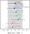 |
Fig. 10. Impact of different cosmic flow correction schemes on H0. The uppermost (black) error bar shows the result from our baseline correction, which uses the 2M++/SDSS velocity field. The other points represent H0 values obtained using alternative correction methods, with vertical positions indicating shifts ΔH0 relative to the baseline. These include a variant of the baseline using additional group redshift corrections from Tully (2015), a variant using the same 2M++ density field but with original parameter choices from Carrick et al. (2015) (C15), a separate reconstruction based on the 2MRS density field, velocity fields derived from the Cf3 and Cf4 galaxy distance catalogues, and a case with no flow correction (CMB frame only). To facilitate comparison, the 68% confidence interval of the baseline is shown as a grey filled band, and its median is marked by grey dashes above and below the other error bars. |
Overall, the different methods exhibit a population standard deviation of 0.5 km s−1 Mpc−1, reflecting a simple estimate of the systematic uncertainty introduced by our choice of flow correction. This is significantly smaller than our baseline statistical error of 1.9 km s−1 Mpc−1, and adding it in quadrature only increases the total uncertainty from 1.9 km s−1 Mpc−1 to 2.0 km s−1 Mpc−1. Finally, we note that these alternative flow corrections also have only a minor effect on the estimated statistical precision of H0, with the width of the 68% confidence interval changing by no more than 3%.
7.1.6. Conclusion of systematic uncertainties
We have identified several systematic uncertainties that could impact our measurement of the Hubble constant: modelling limitations, CSM interaction, the total-to-selective extinction ratio, the photometric system, and peculiar velocities. While we do not find very significant effects from these sources, some uncertainties – for example, those related to the total-to-selective extinction ratio – could be comparable to our statistical uncertainties.
Although we have addressed key systematic uncertainties, our discussion is not exhaustive. For example, we have not considered the possibility of a local Hubble bubble (Zehavi et al. 1998), which could influence measurements at low redshifts and has motivated other analyses (e.g. Riess et al. 2016, 2022) to adopt a larger redshift cutoff.
Overall, while some systematic uncertainties could affect our results at the level of our statistical uncertainties, they are unlikely to significantly alter our main conclusions. With this understanding of our errors, we proceed to compare our measurement of the Hubble constant with those derived from other methods.
7.2. Comparison with other Hubble-constant measurements
In Sect. 6.3, we determined the Hubble constant to be 74.9 ± 1.9 km s−1 Mpc−1, considering only statistical uncertainties. Systematic uncertainties may be of a similar scale (see Sect. 7.1). This is the first H0 determination using the tailored EPM, making it completely independent of existing measurements.
We compare our H0 measurement to other local one-step methods, early universe constraints, and distance ladder results in Fig. 11. Despite our small sample size, our statistical precision of 2.5% is competitive. It matches leading one-step methods such as time-delay lensing by H0LiCOW (Wong et al. 2020) and megamasers from the MCP (Pesce et al. 2020). However, it remains less precise than the best distance-ladder estimates, notably those from SH0ES (Breuval et al. 2024).
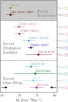 |
Fig. 11. Comparison of our Hubble constant (H0) with other precise, recent measurements. Our result is shown in purple and highlighted with black arrows. Early universe constraints include CMB anisotropies and lensing from Planck (Planck Collaboration VI 2020), as well as a CMB-independent measurement from BAO and BBN (Abbott et al. 2018). Local distance-ladder measurements are shown from the SH0ES project using HST data with Cepheids (Breuval et al. 2024) and from the CCHP project using HST data with the TRGB (Freedman 2021). Additionally, for the newer JWST data, we include results from both SH0ES (Riess et al. 2024) and CCHP (Freedman et al. 2025), where each combines three distance indicators: Cepheids, JAGB stars, and the TRGB. Both projects incorporate systematic uncertainties, added in quadrature, in their measurements using HST and JWST data. We also include another distance-ladder result, which uses SNe II standardised through the SCM and is calibrated by Cepheids and the TRGB (de Jaeger et al. 2022). In contrast to the SH0ES and CCHP measurements, this result does not include systematic uncertainties. For one-step measurements, we show results from time-delay lensing by H0LiCOW (Wong et al. 2020) and TDCOSMO (Birrer et al. 2020), megamasers from the MCP (Pesce et al. 2020), and our own tailored EPM measurement. Compared to the H0LiCOW analysis, TDCOSMO relaxes assumptions on the lens mass models and therefore has larger uncertainties. Among the one-step methods, only the lensing measurements include systematic uncertainties. |
Our small statistical error results from the low dispersion in H0 estimates across different SNe and epochs, highlighting the promise of the tailored EPM. This requires minimal additional uncertainty (σint) beyond the quantified uncertainties. Expanding the sample size and diversity of SNe II will be crucial to confirm this consistency.
Our measurement aligns well with the H0 value reported by SH0ES – the primary local driver of the Hubble tension – and with other precise one-step methods like time-delay lensing and megamasers.
While our results show a moderate 2σ tension with the CCHP results (Freedman 2021; Freedman et al. 2025) based on both HST and JWST data, they indicate a stronger 3.8σ tension with Planck’s H0. However, because systematic errors are not included in our uncertainty budget, this 3.8σ significance is an upper limit. If we assume that systematic uncertainties are comparable to statistical ones, the tension reduces to about 2.7σ.
Regardless of the exact significance, the agreement among the three precise, independent one-step measurements – our tailored EPM, time-delay lensing, and megamasers – provides compelling evidence that the Hubble tension is not simply a product of measurement systematics. This consistency across independent methods suggests that the tension may reflect a genuine discrepancy between local and early universemeasurements.
8. Summary and conclusion
In this work, we present a novel, distance ladder-independent method to determine the Hubble constant using SNe II through the tailored EPM. This approach addresses the ongoing discrepancy between local distance-ladder and early universe measurements of H0. Our tailored EPM technique uses advanced spectral modelling to efficiently fit supernova spectra and derive precise, self-consistent values for luminosity-related parameters. Applying this method to ten SNe II, comprising both literature objects and ePESSTO+ classification targets, with redshifts from 0.01 to 0.04, we find H0 = 74.9 ± 1.9 km s−1 Mpc−1. The quoted uncertainty is statistical. A careful dissection of various dominant sources of systematic effects indicates that systematic errors are likely below or at most comparable to the statistical uncertainties. Our inferred H0 is consistent with most local measurements but in tension with Planck’s early universe constraints.
Our study demonstrates that the tailored EPM achieves a precision comparable to established techniques, such as the TRGB-SN Ia distance ladder and strong lensing, highlighting itspotential as a robust alternative for H0 estimation. However, improvements are needed, particularly in terms of quantifying systematic uncertainties. Key improvements include a better understanding of the modelling uncertainties, especially via comparisons with time-dependent radiative transfer models like CMFGEN, and empirical testing for systematic trends in the distances. The latter requires increased statistical power from more SNe and better constraints from individual objects.
Our current sample faces bottlenecks due to scarce data availability or uncertainties from peculiar motions. For ePESSTO+ objects, peculiar motion uncertainties are mostly small, but the precision is limited by having only one spectrum and photometry in two bands. The literature sample has more spectra and photometry in at least three bands but is constrained by low redshifts, leading to significant uncertainties from peculiar velocities. Future work will focus on higher redshift SNe II with multiple spectroscopic observations and comprehensive multi-band photometry to reduce uncertainties and enhance the reliability of the method.
To address these needs, we have assembled two new datasets for future H0 determinations. The ESO VLT large programme adH0cc26 (Leibundgut et al. 2019) has collected spectral time series (typically four to five spectra per object) and contemporaneous BVRI photometry for around twenty SNe II atredshifts between 0.03 and 0.17. Additionally, the Nearby Supernova Factory (SNfactory; Aldering et al. 2002) has gathered a lower redshift sample (z = 0.01 − 0.04) of another twenty objects. It offers a median of six spectrophotometric observations per object, which will be published in Holas et al. (in prep.). While these objects share similar redshifts with our current sample, the improved data quality and quantity will significantly enhance our analysis.
With a dataset that is four times larger than our current sample and more data per object, these observations will substantially reduce statistical uncertainties and allow more powerful tests for systematic trends. Moreover, these datasets, collected specifically for SN II cosmology and carefully reduced by us, will further minimise observational uncertainties. This includes the uncertainties related to flux calibration and photometric systems, which are better characterised for these single-instrument data. Future analyses will be fully blinded to ensure unbiased results.
These advancements will make our tailored EPM even more valuable in addressing the Hubble tension, providing an independent and precise tool for measuring H0.
Nevertheless, most studies applying the EPM at non-negligible redshifts use the definition of the photospheric angular diameter θ given in Eq. (4) (e.g. Schmidt et al. 1994; Jones et al. 2009). One exception is Gall et al. (2016) who introduce θ† as a new name for the quantity to distinguish it from the true photospheric angular diameter.
This assumes a residual cosmological redshift uncertainty of 250 km s−1 after flow corrections, similar to the Pantheon+ analysis (Brout et al. 2022; Peterson et al. 2022).
We cannot exclude that we missed some objects because the relevant information was not available on WISeREP and the OSC. This applies, in particular, to the early light curve data needed for the time of explosion constraints. Note that after the initial submission of this paper, the CSP sample has been published (Anderson et al. 2024b), which may contain up to three additional suitable objects.
The re-reduced ePESSTO+ classification spectra are available at https://github.com/chvogl/h0-no-rungs-spectral-data/
The filter transmissions and QE can be downloaded from https://github.com/ZwickyTransientFacility/ztf_information
The process of inferring an unknown uncertainty from the data themselves is motivated, for example, in Hogg et al. (2010).
As in Gall et al. (2015) and González-Gaitán et al. (2015), we define the rise time as the time it takes for the magnitude increase to fall below 0.01 mag/day.
For some objects, the spectral observations were taken during the rise of the light curve, requiring us to use data points from this period.
Here σ is the standard deviation of the corresponding full normal distribution.
Plots for the remaining objects can be found in Appendix D.
We performed the correction using the dust_extinction Python package (Gordon 2024).
This is especially the case for the ePESSTO+ SNe with photometry only in g and r, which requires extrapolating the correction significantly to longer and shorter wavelengths.
The impact of extinction on θ/vph is not exactly the same for all epochs due to its interplay with the SN parameters, particularly the temperature.
We excluded the impact of weak gravitational lensing on the flux uncertainties, which is commonly considered in SN cosmological analyses (e.g. Betoule et al. 2014; de Jaeger et al. 2020b; Brout et al. 2022). This effect is negligible for the highest redshifts in our sample, affecting measurements by only about 0.002 mag at z = 0.04 (Jönsson et al. 2010).
Changes in photospheric velocity are not entirely equivalent to red- or blueshifts of the spectrum since they also affect line widths and shapes. However, the effects are similar for small velocity offsets.
If the measured quantities are used, those scattered upwards relative to the true value will receive higher uncertainties and thus lower weight in the fit, while those scattered downwards will receive lower uncertainties and higher weight, biasing the results towards smaller values.
Otherwise, higher H0 values lead to larger θ/vph uncertainties, allowing a wider range of observed data to be accommodated. This increased flexibility results in a greater complexity penalty, thereby reducing the likelihood of higher H0 values.
The colour excesses in g − r and B − V are nearly identical for RV = 3.1.
Accurate determination of H0 with core-collapse supernovae (https://adh0cc.github.io/).
Acknowledgments
Based on observations collected at the European Organisation for Astronomical Research in the Southern Hemisphere, Chile, as part of ePESSTO/ePESSTO+ (the extended Public ESO Spectroscopic Survey for Transient Objects Survey) under ESO programmes 1103.D-0328, 1106.D-0811, and 1108.D-0740. Based on observations obtained with the Samuel Oschin 48-inch Telescope at the Palomar Observatory as part of the Zwicky Transient Facility project. ZTF is supported by the National Science Foundation under Grant No. AST-1440341 and a collaboration including Caltech, IPAC, the Weizmann Institute for Science, the Oskar Klein Center at Stockholm University, the University of Maryland, the University of Washington, Deutsches Elektronen-Synchrotron and Humboldt University, Los Alamos National Laboratories, the TANGO Consortium of Taiwan, the University of Wisconsin at Milwaukee, and Lawrence Berkeley National Laboratories. Operations are conducted by COO, IPAC, and UW. The ZTF forced-photometry service was funded under the Heising-Simons Foundation grant #12540303 (PI: Graham). This work has made use of data from the Asteroid Terrestrial-impact Last Alert System (ATLAS) project. The Asteroid Terrestrial-impact Last Alert System (ATLAS) project is primarily funded to search for near earth asteroids through NASA grants NN12AR55G, 80NSSC18K0284, and 80NSSC18K1575; byproducts of the NEO search include images and catalogs from the survey area. This work was partially funded by Kepler/K2 grant J1944/80NSSC19K0112 and HST GO-15889, and STFC grants ST/T000198/1 and ST/S006109/1. The ATLAS science products have been made possible through the contributions of the University of Hawaii Institute for Astronomy, the Queen’s University Belfast, the Space Telescope Science Institute, the South African Astronomical Observatory, and The Millennium Institute of Astrophysics (MAS), Chile. The authors would like to acknowledge the use of ChatGPT (version 4.0 and 4.01-preview) developed by OpenAI for assisting with language editing of this manuscript. The model’s capabilities were employed to improve clarity, grammar, and coherence in several sections of the text. This research has made use of the NASA/IPAC Extragalactic Database (NED), which is operated by the Jet Propulsion Laboratory, California Institute of Technology, under contract with the National Aeronautics and Space Administration. This research made use of TARDIS, a community-developed software package for spectral synthesis in supernovae (Kerzendorf & Sim 2014; Kerzendorf et al. 2023). The development of TARDIS received support from GitHub, the Google Summer of Code initiative, and from ESA’s Summer of Code in Space program. TARDIS is a fiscally sponsored project of NumFOCUS. TARDIS makes extensive use of Astropy and Pyne. This research is supported in part by the Excellence Cluster ORIGINS, which is funded by the Deutsche Forschungsgemeinschaft (DFG, German Research Foundation) under Germany’s Excellence Strategy-EXC-2094-390783311. This work was supported by the Action Thémathique de Physique Stellaire (ATPS) of CNRS/INSU PN Astro cofunded by CEA and CNES. AH acknowledges support by the Klaus Tschira Foundation. AH is a Fellow of the International Max Planck Research School for Astronomy and Cosmic Physics at the University of Heidelberg (IMPRS-HD). AF acknowledges support by the European Research Council (ERC) under the European Union’s Horizon 2020 research and innovation program (ERC Advanced Grant KILONOVA No. 885281) and the State of Hesse within the Cluster Project ELEMENTS. JVS is supported by the National Science Foundation under Grant No. OAC-2311323 and through the U.S. Department of Energy, Office of Science, Office of Nuclear Physics, award No. DE-SC0017955. SHS thanks the Max Planck Society for support through the Max Planck Fellowship. The authors thank Joe Lyman und Matt Nicholl for taking the calibration data needed for the EFOSC2 second order correction. In addition, they are grateful to Mickael Rigault for sharing valuable insights on the ZTF pocket effect. Contributor roles according to the CRediT standard: (https://credit.niso.org/). Conceptualization: W. Hillebrandt, B. Leibundgut, C. Vogl, S. Taubenberger. Data curation, formal analysis, and visualization: C. Vogl. Funding acquisition and resources: W. Hillebrandt, S. H. Suyu. Investigation, methodology, and validation: C. Vogl, S. Taubenberger, E. R. Peterson, H. M. Courtois. Project administration: C. Vogl, W. Hillebrandt, B. Leibundgut. Software: C. Vogl, W. E. Kerzendorf, S. A. Sim. Supervision: W. Hillebrandt, S. H. Suyu, B. Leibundgut, W. E. Kerzendorf, S. A. Sim. Writing – original draft: C. Vogl, G. Csörnyei. Writing – review & editing: C. Vogl, S. Taubenberger, G. Csörnyei, B. Leibundgut, W. E. Kerzendorf, S. A. Sim, S. Blondin, A. Flörs, A. Holas, J. V. Shields, J. Spyromilio, S. H. Suyu, W. Hillebrandt.
References
- Abbott, T. M. C., Abdalla, F. B., Annis, J., et al. 2018, MNRAS, 480, 3879 [Google Scholar]
- Aiola, S., Calabrese, E., Maurin, L., et al. 2020, JCAP, 2020, 047 [Google Scholar]
- Aldering, G., Adam, G., Antilogus, P., et al. 2002, in Overview of the Nearby Supernova Factory, eds. J. A. Tyson, & S. Wolff, SPIE Conf. Ser., 4836, 61 [Google Scholar]
- Ambikasaran, S., Foreman-Mackey, D., Greengard, L., Hogg, D. W., & O’Neil, M. 2015, IEEE Trans. Pattern Anal. Mach. Intell., 38, 252 [Google Scholar]
- Anand, G. S., Tully, R. B., Rizzi, L., Riess, A. G., & Yuan, W. 2022, ApJ, 932, 15 [NASA ADS] [CrossRef] [Google Scholar]
- Anderson, J. P., González-Gaitán, S., Hamuy, M., et al. 2014, ApJ, 786, 67 [Google Scholar]
- Anderson, R. I., Koblischke, N. W., & Eyer, L. 2024a, ApJ, 963, L43 [NASA ADS] [CrossRef] [Google Scholar]
- Anderson, J. P., Contreras, C., Stritzinger, M. D., et al. 2024b, A&A, 692, A95 [NASA ADS] [CrossRef] [EDP Sciences] [Google Scholar]
- Astier, P., Guy, J., Regnault, N., et al. 2006, A&A, 447, 31 [NASA ADS] [CrossRef] [EDP Sciences] [Google Scholar]
- Baron, E., Nugent, P. E., Branch, D., & Hauschildt, P. H. 2004, ApJ, 616, L91 [NASA ADS] [CrossRef] [Google Scholar]
- Bazin, G., Palanque-Delabrouille, N., Rich, J., et al. 2009, A&A, 499, 653 [NASA ADS] [CrossRef] [EDP Sciences] [Google Scholar]
- Bellm, E. C., Kulkarni, S. R., Graham, M. J., et al. 2019, PASP, 131, 018002 [Google Scholar]
- Berbig, M., Jana, S., & Trautner, A. 2020, Phys. Rev. D, 102, 115008 [Google Scholar]
- Bessell, M., & Murphy, S. 2012, PASP, 124, 140 [NASA ADS] [CrossRef] [Google Scholar]
- Betoule, M., Kessler, R., Guy, J., et al. 2014, A&A, 568, A22 [NASA ADS] [CrossRef] [EDP Sciences] [Google Scholar]
- Birrer, S., Shajib, A. J., Galan, A., et al. 2020, A&A, 643, A165 [NASA ADS] [CrossRef] [EDP Sciences] [Google Scholar]
- Bishop, C. M., & Nasrabadi, N. M. 2007, J. Electron. Imaging, 16, 049901 [NASA ADS] [CrossRef] [Google Scholar]
- Blakeslee, J. P., Jensen, J. B., Ma, C.-P., Milne, P. A., & Greene, J. E. 2021, ApJ, 911, 65 [NASA ADS] [CrossRef] [Google Scholar]
- Blondin, S., Davis, T. M., Krisciunas, K., et al. 2008, ApJ, 682, 724 [Google Scholar]
- Breuval, L., Riess, A. G., Kervella, P., Anderson, R. I., & Romaniello, M. 2022, ApJ, 939, 89 [NASA ADS] [CrossRef] [Google Scholar]
- Breuval, L., Riess, A. G., Casertano, S., et al. 2024, ApJ, 973, 30 [Google Scholar]
- Brout, D., Scolnic, D., Popovic, B., et al. 2022, ApJ, 938, 110 [NASA ADS] [CrossRef] [Google Scholar]
- Bruch, R. J., Gal-Yam, A., Schulze, S., et al. 2021, ApJ, 912, 46 [NASA ADS] [CrossRef] [Google Scholar]
- Bruch, R. J., Gal-Yam, A., Yaron, O., et al. 2023, ApJ, 952, 119 [NASA ADS] [CrossRef] [Google Scholar]
- Buzzoni, B., Delabre, B., Dekker, H., et al. 1984, Messenger, 38, 9 [Google Scholar]
- Carr, A., Davis, T. M., Scolnic, D., et al. 2022, PASA, 39, e046 [NASA ADS] [CrossRef] [Google Scholar]
- Carrick, J., Turnbull, S. J., Lavaux, G., & Hudson, M. J. 2015, MNRAS, 450, 317 [Google Scholar]
- Chen, G. C. F., Fassnacht, C. D., Suyu, S. H., et al. 2019, MNRAS, 490, 1743 [NASA ADS] [CrossRef] [Google Scholar]
- Ciddor, P. E. 1996, Appl. Opt., 35, 1566 [Google Scholar]
- Courtois, H. M., Dupuy, A., Guinet, D., et al. 2023, A&A, 670, L15 [NASA ADS] [CrossRef] [EDP Sciences] [Google Scholar]
- Csörnyei, G., Vogl, C., Taubenberger, S., et al. 2023a, A&A, 672, A129 [NASA ADS] [CrossRef] [EDP Sciences] [Google Scholar]
- Csörnyei, G., Anderson, R. I., Vogl, C., et al. 2023b, A&A, 678, A44 [NASA ADS] [CrossRef] [EDP Sciences] [Google Scholar]
- Czekala, I., Andrews, S. M., Mandel, K. S., Hogg, D. W., & Green, G. M. 2015, ApJ, 812, 128 [NASA ADS] [CrossRef] [Google Scholar]
- Davis, T. M., & Scrimgeour, M. I. 2014, MNRAS, 442, 1117 [NASA ADS] [CrossRef] [Google Scholar]
- de Jaeger, T., & Galbany, L. 2024, in The Pursuit of the Hubble Constant Using Type II Supernovae, eds. E. Di Valentino, & D. Brout (Singapore: Springer Nature), 177 [Google Scholar]
- de Jaeger, T., González-Gaitán, S., Anderson, J. P., et al. 2015, ApJ, 815, 121 [NASA ADS] [CrossRef] [Google Scholar]
- de Jaeger, T., González-Gaitán, S., Hamuy, M., et al. 2017, ApJ, 835, 166 [NASA ADS] [CrossRef] [Google Scholar]
- de Jaeger, T., Zheng, W., Stahl, B. E., et al. 2019, MNRAS, 490, 2799 [NASA ADS] [CrossRef] [Google Scholar]
- de Jaeger, T., Stahl, B. E., Zheng, W., et al. 2020a, MNRAS, 496, 3402 [NASA ADS] [CrossRef] [Google Scholar]
- de Jaeger, T., Galbany, L., González-Gaitán, S., et al. 2020b, MNRAS, 495, 4860 [NASA ADS] [CrossRef] [Google Scholar]
- de Jaeger, T., Galbany, L., Riess, A. G., et al. 2022, MNRAS, 514, 4620 [NASA ADS] [CrossRef] [Google Scholar]
- Dessart, L., & Hillier, D. J. 2005, A&A, 437, 667 [NASA ADS] [CrossRef] [EDP Sciences] [Google Scholar]
- Dessart, L., & Hillier, D. J. 2006, A&A, 447, 691 [NASA ADS] [CrossRef] [EDP Sciences] [Google Scholar]
- Dessart, L., & Hillier, D. J. 2011, MNRAS, 410, 1739 [NASA ADS] [Google Scholar]
- Dessart, L., & Jacobson-Galán, W. V. 2023, A&A, 677, A105 [NASA ADS] [CrossRef] [EDP Sciences] [Google Scholar]
- Dessart, L., Blondin, S., Brown, P. J., et al. 2008, ApJ, 675, 644 [NASA ADS] [CrossRef] [Google Scholar]
- Dhawan, S., Jha, S. W., & Leibundgut, B. 2018, A&A, 609, A72 [NASA ADS] [CrossRef] [EDP Sciences] [Google Scholar]
- Dhungana, G., Kehoe, R., Staten, R., et al. 2024, ApJ, 962, 60 [Google Scholar]
- Di Valentino, E., Mena, O., Pan, S., et al. 2021, Classical Quantum Gravity, 38, 153001 [Google Scholar]
- Doi, M., Tanaka, M., Fukugita, M., et al. 2010, AJ, 139, 1628 [NASA ADS] [CrossRef] [Google Scholar]
- Dutcher, D., Balkenhol, L., Ade, P. A. R., et al. 2021, Phys. Rev. D, 104, 022003 [NASA ADS] [CrossRef] [Google Scholar]
- Eastman, R. G., Schmidt, B. P., & Kirshner, R. 1996, ApJ, 466, 911 [NASA ADS] [CrossRef] [Google Scholar]
- Fitzpatrick, E. L., Massa, D., Gordon, K. D., Bohlin, R., & Clayton, G. C. 2019, ApJ, 886, 108 [Google Scholar]
- Foreman-Mackey, D. 2016, J. Open Source Softw., 1, 24 [Google Scholar]
- Freedman, W. L. 2021, ApJ, 919, 16 [NASA ADS] [CrossRef] [Google Scholar]
- Freedman, W. L., Madore, B. F., Hatt, D., et al. 2019, ApJ, 882, 34 [Google Scholar]
- Freedman, W. L., Madore, B. F., Hoyt, T., et al. 2020, ApJ, 891, 57 [Google Scholar]
- Freedman, W. L., Madore, B. F., Jang, I. S., et al. 2025, ApJ, 985, 203 [Google Scholar]
- Fuller, J. 2017, MNRAS, 470, 1642 [NASA ADS] [CrossRef] [Google Scholar]
- Fuller, J., & Tsuna, D. 2024, Open J. Astrophys., 7, 47 [CrossRef] [Google Scholar]
- Galbany, L., Hamuy, M., Phillips, M. M., et al. 2016, AJ, 151, 33 [NASA ADS] [CrossRef] [Google Scholar]
- Gall, E. E. E., Polshaw, J., Kotak, R., et al. 2015, A&A, 582, A3 [NASA ADS] [CrossRef] [EDP Sciences] [Google Scholar]
- Gall, E. E. E., Kotak, R., Leibundgut, B., et al. 2016, A&A, 592, A129 [NASA ADS] [CrossRef] [EDP Sciences] [Google Scholar]
- Gall, E. E. E., Kotak, R., Leibundgut, B., et al. 2018, A&A, 611, A25 [NASA ADS] [CrossRef] [EDP Sciences] [Google Scholar]
- Gal-Yam, A., Kasliwal, M. M., Arcavi, I., et al. 2011, ApJ, 736, 159 [NASA ADS] [CrossRef] [Google Scholar]
- Ganeshalingam, M., Li, W., Filippenko, A. V., et al. 2010, ApJS, 190, 418 [NASA ADS] [CrossRef] [Google Scholar]
- Ginolin, M., Rigault, M., Smith, M., et al. 2025, A&A, 695, A140 [NASA ADS] [CrossRef] [EDP Sciences] [Google Scholar]
- Goldstein, D. A., Nugent, P. E., & Goobar, A. 2019, ApJS, 243, 6 [NASA ADS] [CrossRef] [Google Scholar]
- González-Gaitán, S., Tominaga, N., Molina, J., et al. 2015, MNRAS, 451, 2212 [CrossRef] [Google Scholar]
- Gordon, K. 2024, https://doi.org/10.5281/zenodo.4658887 [Google Scholar]
- Graziani, R., Courtois, H. M., Lavaux, G., et al. 2019, MNRAS, 488, 5438 [NASA ADS] [CrossRef] [Google Scholar]
- Grillo, C., Pagano, L., Rosati, P., & Suyu, S. H. 2024, A&A, 684, L23 [NASA ADS] [CrossRef] [EDP Sciences] [Google Scholar]
- Guillochon, J., Parrent, J., Kelley, L. Z., & Margutti, R. 2017, ApJ, 835, 64 [Google Scholar]
- Gutiérrez, C. P., Anderson, J. P., Hamuy, M., et al. 2017a, ApJ, 850, 89 [CrossRef] [Google Scholar]
- Gutiérrez, C. P., Anderson, J. P., Hamuy, M., et al. 2017b, ApJ, 850, 90 [CrossRef] [Google Scholar]
- Hamuy, M., & Pinto, P. A. 2002, ApJ, 566, L63 [NASA ADS] [CrossRef] [Google Scholar]
- Hatano, K., Branch, D., & Deaton, J. 1998, ApJ, 502, 177 [Google Scholar]
- Herold, L., & Ferreira, E. G. M. 2023, Phys. Rev. D, 108, 043513 [Google Scholar]
- Hicken, M., Challis, P., Jha, S., et al. 2009, ApJ, 700, 331 [Google Scholar]
- Hicken, M., Friedman, A. S., Blondin, S., et al. 2017, ApJS, 233, 6 [NASA ADS] [CrossRef] [Google Scholar]
- Hillier, D. J., & Dessart, L. 2019, A&A, 631, A8 [NASA ADS] [CrossRef] [EDP Sciences] [Google Scholar]
- Hinshaw, G., Larson, D., Komatsu, E., et al. 2013, ApJS, 208, 19 [Google Scholar]
- Hogg, D. W. 1999, ArXiv e-prints [arXiv:astro-ph/9905116] [Google Scholar]
- Hogg, D. W., Baldry, I. K., Blanton, M. R., & Eisenstein, D. J. 2002, ArXiv e-prints [arXiv:astro-ph/0210394] [Google Scholar]
- Hogg, D. W., Bovy, J., & Lang, D. 2010, ArXiv e-prints [arXiv:1008.4686] [Google Scholar]
- Hoyt, T. J. 2023, Nat. Astron., 7, 590 [NASA ADS] [CrossRef] [Google Scholar]
- Hoyt, T. J., Jang, I. S., Freedman, W. L., et al. 2024, ApJ, 975, 111 [Google Scholar]
- Huang, C. D., Riess, A. G., Yuan, W., et al. 2020, ApJ, 889, 5 [Google Scholar]
- Huang, C. D., Yuan, W., Riess, A. G., et al. 2024, ApJ, 963, 83 [Google Scholar]
- Huchra, J. P., Macri, L. M., Masters, K. L., et al. 2012, ApJS, 199, 26 [Google Scholar]
- Inserra, C., Smartt, S. J., Gall, E. E. E., et al. 2018, MNRAS, 475, 1046 [NASA ADS] [CrossRef] [Google Scholar]
- Jacobson-Galán, W. V., Dessart, L., Margutti, R., et al. 2023, ApJ, 954, L42 [CrossRef] [Google Scholar]
- Jacobson-Galán, W. V., Dessart, L., Davis, K. W., et al. 2024, ApJ, 970, 189 [CrossRef] [Google Scholar]
- Jha, S., Riess, A. G., & Kirshner, R. P. 2007, ApJ, 659, 122 [NASA ADS] [CrossRef] [Google Scholar]
- Johansson, J., Cenko, S. B., Fox, O. D., et al. 2021, ApJ, 923, 237 [NASA ADS] [CrossRef] [Google Scholar]
- Jones, M. I., Hamuy, M., Lira, P., et al. 2009, ApJ, 696, 1176 [NASA ADS] [CrossRef] [Google Scholar]
- Jönsson, J., Sullivan, M., Hook, I., et al. 2010, MNRAS, 405, 535 [NASA ADS] [Google Scholar]
- Kangas, T., Yan, L., Schulze, S., et al. 2022, MNRAS, 516, 1193 [Google Scholar]
- Kelly, P. L., Rodney, S., Treu, T., et al. 2023, Science, 380, abh1322 [NASA ADS] [CrossRef] [Google Scholar]
- Kerzendorf, W. E., & Sim, S. A. 2014, MNRAS, 440, 387 [NASA ADS] [CrossRef] [Google Scholar]
- Kerzendorf, W., Sim, S., Vogl, C., et al. 2023, https://doi.org/10.5281/zenodo.8244935 [Google Scholar]
- Khazov, D., Yaron, O., Gal-Yam, A., et al. 2016, ApJ, 818, 3 [CrossRef] [Google Scholar]
- Kirshner, R. P., & Kwan, J. 1974, ApJ, 193, 27 [NASA ADS] [CrossRef] [Google Scholar]
- Koblischke, N. W., & Anderson, R. I. 2024, ApJ, 974, 181 [Google Scholar]
- Kreisch, C. D., Cyr-Racine, F.-Y., & Doré, O. 2020, Phys. Rev. D, 101, 123505 [Google Scholar]
- Lee, N., & Li, W. 2006, CBETs, 660, 1 [Google Scholar]
- Lee, A. J., Freedman, W. L., Madore, B. F., et al. 2025, ApJ, 985, 182 [Google Scholar]
- Léget, P. F., Pruzhinskaya, M. V., Ciulli, A., et al. 2018, A&A, 615, A162 [NASA ADS] [CrossRef] [EDP Sciences] [Google Scholar]
- Leibundgut, B., Schommer, R., Phillips, M., et al. 1996, ApJ, 466, L21 [Google Scholar]
- Leibundgut, B., Spyromilio, J., Vogl, C., et al. 2019, TNSAN, 103, 1 [Google Scholar]
- Lilow, R., & Nusser, A. 2021, MNRAS, 507, 1557 [NASA ADS] [CrossRef] [Google Scholar]
- Madore, B. F., & Freedman, W. L. 2020, ApJ, 899, 66 [NASA ADS] [CrossRef] [Google Scholar]
- Madore, B. F., & Freedman, W. L. 2024, ApJ, 961, 166 [Google Scholar]
- Masci, F. J., Laher, R. R., Rusholme, B., et al. 2019, PASP, 131, 018003 [Google Scholar]
- Masci, F. J., Laher, R. R., Rusholme, B., et al. 2023, ArXiv e-prints [arXiv:2305.16279] [Google Scholar]
- Millon, M., Galan, A., Courbin, F., et al. 2020, A&A, 639, A101 [NASA ADS] [CrossRef] [EDP Sciences] [Google Scholar]
- Morozova, V., Piro, A. L., & Valenti, S. 2017, ApJ, 838, 28 [NASA ADS] [CrossRef] [Google Scholar]
- Mörtsell, E., Goobar, A., Johansson, J., & Dhawan, S. 2022a, ApJ, 933, 212 [CrossRef] [Google Scholar]
- Mörtsell, E., Goobar, A., Johansson, J., & Dhawan, S. 2022b, ApJ, 935, 58 [CrossRef] [Google Scholar]
- Ofek, E. O., Arcavi, I., Tal, D., et al. 2014, ApJ, 788, 154 [NASA ADS] [CrossRef] [Google Scholar]
- Pan, S., & Yang, W. 2024, in On the Interacting Dark Energy Scenarios–The Case for Hubble Constant Tension, eds. E. Di Valentino, & D. Brout (Singapore: Springer Nature Singapore), 531 [Google Scholar]
- Pascale, M., Frye, B. L., Pierel, J. D. R., et al. 2025, ApJ, 979, 13 [Google Scholar]
- Pesce, D. W., Braatz, J. A., Reid, M. J., et al. 2020, ApJ, 891, L1 [Google Scholar]
- Peterson, E. R., Kenworthy, W. D., Scolnic, D., et al. 2022, ApJ, 938, 112 [NASA ADS] [CrossRef] [Google Scholar]
- Planck Collaboration I. 2020, A&A, 641, A1 [NASA ADS] [CrossRef] [EDP Sciences] [Google Scholar]
- Planck Collaboration VI. 2020, A&A, 641, A6 [NASA ADS] [CrossRef] [EDP Sciences] [Google Scholar]
- Poulin, V., Smith, T. L., Karwal, T., & Kamionkowski, M. 2019, Phys. Rev. Lett., 122, 221301 [Google Scholar]
- Rasmussen, C. E., & Williams, C. K. I. 2006, Gaussian Processes for Machine Learning (The MIT Press) [Google Scholar]
- Reid, M. J., Pesce, D. W., & Riess, A. G. 2019, ApJ, 886, L27 [Google Scholar]
- Riess, A. G., Strolger, L.-G., Tonry, J., et al. 2004, ApJ, 607, 665 [NASA ADS] [CrossRef] [Google Scholar]
- Riess, A. G., Macri, L. M., Hoffmann, S. L., et al. 2016, ApJ, 826, 56 [Google Scholar]
- Riess, A. G., Yuan, W., Macri, L. M., et al. 2022, ApJ, 934, L7 [NASA ADS] [CrossRef] [Google Scholar]
- Riess, A. G., Scolnic, D., Anand, G. S., et al. 2024, ApJ, 977, 120 [NASA ADS] [CrossRef] [Google Scholar]
- Rigault, M., Smith, M., Goobar, A., et al. 2025, A&A, 694, A1 [NASA ADS] [CrossRef] [EDP Sciences] [Google Scholar]
- Rodríguez, Ó., Clocchiatti, A., & Hamuy, M. 2014, AJ, 148, 107 [CrossRef] [Google Scholar]
- Rodríguez, Ó., Pignata, G., Hamuy, M., et al. 2019, MNRAS, 483, 5459 [CrossRef] [Google Scholar]
- Rubin, D., Aldering, G., Barbary, K., et al. 2015, ApJ, 813, 137 [Google Scholar]
- Rubin, A., Gal-Yam, A., De Cia, A., et al. 2016, ApJ, 820, 33 [NASA ADS] [CrossRef] [Google Scholar]
- Rubin, D., Aldering, G., Betoule, M., et al. 2025, ApJ, 986, 231 [Google Scholar]
- Said, K., Colless, M., Magoulas, C., Lucey, J. R., & Hudson, M. J. 2020, MNRAS, 497, 1275 [NASA ADS] [CrossRef] [Google Scholar]
- Salim, S., Boquien, M., & Lee, J. C. 2018, ApJ, 859, 11 [Google Scholar]
- Sandage, A., & Tammann, G. A. 1974, ApJ, 190, 525 [Google Scholar]
- Schlafly, E. F., & Finkbeiner, D. P. 2011, ApJ, 737, 103 [Google Scholar]
- Schlafly, E. F., Meisner, A. M., Stutz, A. M., et al. 2016, ApJ, 821, 78 [NASA ADS] [CrossRef] [Google Scholar]
- Schmidt, B. P., Kirshner, R. P., & Eastman, R. G. 1992, ApJ, 395, 366 [NASA ADS] [CrossRef] [Google Scholar]
- Schmidt, B. P., Kirshner, R. P., Eastman, R. G., et al. 1994, ApJ, 432, 42 [NASA ADS] [CrossRef] [Google Scholar]
- Schombert, J., McGaugh, S., & Lelli, F. 2020, AJ, 160, 71 [NASA ADS] [CrossRef] [Google Scholar]
- Schöneberg, N., Lesgourgues, J., & Hooper, D. C. 2019, JCAP, 2019, 029 [CrossRef] [Google Scholar]
- Schöneberg, N., Abellán, G. F., Sánchez, A. P., et al. 2022, Phys. Rep., 984, 1 [CrossRef] [Google Scholar]
- Scolnic, D. M., Jones, D. O., Rest, A., et al. 2018, ApJ, 859, 101 [NASA ADS] [CrossRef] [Google Scholar]
- Scolnic, D., Riess, A. G., Wu, J., et al. 2023, ApJ, 954, L31 [NASA ADS] [CrossRef] [Google Scholar]
- Shajib, A. J., Birrer, S., Treu, T., et al. 2020, MNRAS, 494, 6072 [Google Scholar]
- Shajib, A. J., Mozumdar, P., Chen, G. C. F., et al. 2023, A&A, 673, A9 [NASA ADS] [CrossRef] [EDP Sciences] [Google Scholar]
- Shingles, L., Smith, K. W., Young, D. R., et al. 2021, TNSAN, 7, 1 [NASA ADS] [Google Scholar]
- Smartt, S. J., Valenti, S., Fraser, M., et al. 2015, A&A, 579, A40 [NASA ADS] [CrossRef] [EDP Sciences] [Google Scholar]
- Smith, J. A., Tucker, D. L., Kent, S., et al. 2002, AJ, 123, 2121 [NASA ADS] [CrossRef] [Google Scholar]
- Smith, T. L., Poulin, V., & Amin, M. A. 2020a, Phys. Rev. D, 101, 063523 [Google Scholar]
- Smith, K. W., Smartt, S. J., Young, D. R., et al. 2020b, PASP, 132, 085002 [Google Scholar]
- Stanishev, V. 2007, Astron. Nachr., 328, 948 [Google Scholar]
- Suyu, S. H., Bonvin, V., Courbin, F., et al. 2017, MNRAS, 468, 2590 [Google Scholar]
- Suyu, S. H., Huber, S., Cañameras, R., et al. 2020, A&A, 644, A162 [NASA ADS] [CrossRef] [EDP Sciences] [Google Scholar]
- Taubenberger, S., Suyu, S. H., Komatsu, E., et al. 2019, A&A, 628, L7 [NASA ADS] [CrossRef] [EDP Sciences] [Google Scholar]
- Taylor, M., Cinabro, D., Dilday, B., et al. 2014, ApJ, 792, 135 [Google Scholar]
- Teja, R. S., Singh, A., Basu, J., et al. 2023, ApJ, 954, L12 [NASA ADS] [CrossRef] [Google Scholar]
- Thorp, S., Mandel, K. S., Jones, D. O., Kirshner, R. P., & Challis, P. M. 2024, MNRAS, 530, 4016 [NASA ADS] [CrossRef] [Google Scholar]
- Tody, D. 1986, in Instrumentation in Astronomy VI, ed. D. L. Crawford, SPIE Conf. Ser., 627, 733 [NASA ADS] [CrossRef] [Google Scholar]
- Tody, D. 1993, in Astronomical Data Analysis Software and Systems II, eds. R. J. Hanisch, R. J. V. Brissenden, & J. Barnes, ASP Conf. Ser., 52, 173 [Google Scholar]
- Tonry, J. L., Denneau, L., Heinze, A. N., et al. 2018, PASP, 130, 064505 [Google Scholar]
- Tully, R. B. 2015, AJ, 149, 171 [NASA ADS] [CrossRef] [Google Scholar]
- Tully, R. B., Courtois, H. M., & Sorce, J. G. 2016, AJ, 152, 50 [Google Scholar]
- Tully, R. B., Kourkchi, E., Courtois, H. M., et al. 2023, ApJ, 944, 94 [NASA ADS] [CrossRef] [Google Scholar]
- Uddin, S. A., Burns, C. R., Phillips, M. M., et al. 2024, ApJ, 970, 72 [Google Scholar]
- Valenti, S., Howell, D. A., Stritzinger, M. D., et al. 2016, MNRAS, 459, 3939 [NASA ADS] [CrossRef] [Google Scholar]
- van Dokkum, P. G. 2001, PASP, 113, 1420 [Google Scholar]
- Vasylyev, S. S., Filippenko, A. V., Vogl, C., et al. 2022, ApJ, 934, 134 [NASA ADS] [CrossRef] [Google Scholar]
- Vasylyev, S. S., Vogl, C., Yang, Y., et al. 2023, ApJ, 959, L26 [Google Scholar]
- Verde, L., Schöneberg, N., & Gil-Marín, H. 2024, ARA&A, 62, 287 [Google Scholar]
- Vincenzi, M., Sullivan, M., Möller, A., et al. 2023, MNRAS, 518, 1106 [Google Scholar]
- Vogl, C., Sim, S. A., Noebauer, U. M., Kerzendorf, W. E., & Hillebrandt, W. 2019, A&A, 621, A29 [NASA ADS] [CrossRef] [EDP Sciences] [Google Scholar]
- Vogl, C., Kerzendorf, W. E., Sim, S. A., et al. 2020, A&A, 633, A88 [NASA ADS] [CrossRef] [EDP Sciences] [Google Scholar]
- Wagoner, R. V. 1981, ApJ, 250, L65 [Google Scholar]
- Wang, B., Abdalla, E., Atrio-Barandela, F., & Pavón, D. 2016, Rep. Progr. Phys., 79, 096901 [Google Scholar]
- Wojtak, R., Hjorth, J., & Hjortlund, J. O. 2023, MNRAS, 525, 5187 [NASA ADS] [CrossRef] [Google Scholar]
- Wong, K. C., Suyu, S. H., Chen, G. C. F., et al. 2020, MNRAS, 498, 1420 [Google Scholar]
- Wong, K. C., Dux, F., Shajib, A. J., et al. 2024, A&A, 689, A168 [NASA ADS] [CrossRef] [EDP Sciences] [Google Scholar]
- Wood-Vasey, W. M., Aldering, G., Nugent, P., Mulchaey, J., & Phillips, M. 2003, IAU Circ., 8088, 2 [Google Scholar]
- Yao, Y., De, K., Kasliwal, M. M., et al. 2020, ApJ, 900, 46 [NASA ADS] [CrossRef] [Google Scholar]
- Yaron, O., & Gal-Yam, A. 2012, PASP, 124, 668 [Google Scholar]
- Yaron, O., Perley, D. A., Gal-Yam, A., et al. 2017, Nat. Phys., 13, 510 [NASA ADS] [CrossRef] [Google Scholar]
- Yıldırım, A., Suyu, S. H., Chen, G. C. F., & Komatsu, E. 2023, A&A, 675, A21 [NASA ADS] [CrossRef] [EDP Sciences] [Google Scholar]
- Zehavi, I., Riess, A. G., Kirshner, R. P., & Dekel, A. 1998, ApJ, 503, 483 [Google Scholar]
Appendix A: Spectroscopic and photometric data
Log of modelled spectra and corresponding interpolated photometry.
Appendix B: Time of explosion
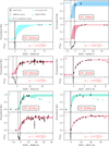 |
Fig. B.1. Time-of-explosion fits for a first set of six SNe. For SN 2006it, the r-band data – showing the SN on its plateau – provide additional constraints on the clear-band rise through our prior te, clear < te, r. |
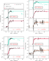 |
Fig. B.2. Time-of-explosion fits for a second set of four SNe. See Fig. 2 for an explanation of the plot. |
Appendix C: Light curve interpolation
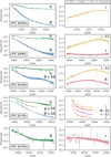 |
Fig. C.1. GP interpolation of the photometry for the first five SNe in the sample. See Fig. 3 for an explanation of the plot. Each row corresponds to one SN. Compared to Fig. 3, multiple bands are shown per panel, with bluer bands on the left and redder bands on the right. Some bands are offset for visual clarity; offsets are indicated in the plot. |
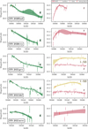 |
Fig. C.2. GP interpolation of the photometry for the remaining five SNe in the sample. See Fig. 3 for an explanation of the plot. Each row corresponds to one SN. Compared to Fig. 3, multiple bands are shown per panel, with bluer bands on the left and redder bands on the right. Some bands are offset for visual clarity; offsets are indicated in the plot. |
Appendix D: Flux calibration
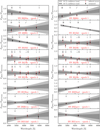 |
Fig. D.1. Linear flux calibration procedure for the full SN sample. See Fig. 4 for an explanation of the plot. |
Appendix E: Spectral fits
Appendix F: Peculiar velocities
Peculiar velocities and Tully (2015) group redshifts used in Sect. 7.1.5.
All Tables
All Figures
|
Fig. 1. EPM regression principle. The EPM uses multiple spectroscopic observations to measure the ratio of the photospheric angular diameter θ (Eq. (4)) and the photospheric velocity vph for different times. These measurements (shown in blue) fall on a straight line (red). We can determine the SN luminosity distance DL from the inverse of the slope of this line and the time of explosion from the intercept (see Eq. (5)). |
| In the text | |
|
Fig. 2. Example of the time-of-explosion determination. We fitted an inverse exponential model (Eq. (8)) to the observed flux curves (black error bars), modelling the available bands (here g and r) jointly with a shared explosion time t0. The coloured bands (cyan for g, red for r) show the 95% confidence regions of the fits. The bottom panel displays the t0 posterior along with the inferred value relative to the first detection and its uncertainty. Finally, the inflated flux errors, including the additional fitted uncertainty σadd, are shown in grey. Here, the reported g-band uncertainties accurately capture the scatter around the model, resulting in minimal error inflation. In contrast, the r-band errors show noticeable inflation, with σadd around 0.06 mag. |
| In the text | |
|
Fig. 3. Example of the GP interpolation of the photometry. We plot the observed magnitudes and their uncertainties in black; the interpolated values at the spectral epochs are shown in red. The coloured bands, finally, indicate the 68% confidence interval of the interpolated light curve and the dashed line the median. |
| In the text | |
|
Fig. 4. Example of the linear flux calibration procedure. The plot shows the measured ratios of the photometric and spectroscopic flux Fphot/Fspectrum for the first epoch of SN 2006it as a function of wavelength in black. We performed a Bayesian fit of the ratios (see Sect. 4.3) to identify all possible linear flux calibration corrections. Of the possible curves 68% fall within the dark grey contour and 95% within the light grey contour. Although the underlying curves are straight, the contours naturally exhibit curvature. An important part of the fit is inflating the measured errors if necessary, accounting for additional unquantified uncertainties, such as the mixing of different photometric systems or underestimated uncertainties in the interpolated magnitudes. In the plot, the inflated errors are highlighted in red. In this specific example, the errors are substantially inflated because the data points deviate significantly from a linear trend within the measurement uncertainties. |
| In the text | |
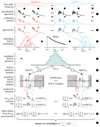 |
Fig. 5. Procedure to determine θ/vph and E(B − V) as described in Sect. 5. |
| In the text | |
|
Fig. 6. Example spectral fits. We show the spectral fits for SN 2006it at two epochs (Oct. 10 and Oct. 13), analogous to the hypothetical SN used in Fig. 5. The bottom panel displays the E(B − V) constraints from spectral fits of possible flux calibration solutions, with epoch 1 in blue and epoch 2 in green. The constraints from both epochs align well within the uncertainties. The dashed black line represents the exponential approximation of the Hatano et al. (1998) extinction prior, with dots indicating evaluation points for multiplication with the individual epoch constraints. We plot the final E(B − V) posterior (red) in the negative probability density direction for visual separation. The upper part of the figure visualises the spectral fits contributing to the E(B − V) and subsequently θ/vph determinations. While fits of many different flux-calibrated spectra and E(B − V) values contribute, we show only one representative fit per epoch for simplicity. To select this fit, we follow a two-step process. First, we choose one of the flux calibration solutions whose best-fit E(B − V) is closest to the median of the posterior. Next, within this flux calibration solution, we analogously identify the fit from the E(B − V) grid that is nearest to the median of the posterior. The normalised observed specific flux fλ of this choice appears in black, with the corresponding maximum-likelihood fits in blue (epoch 1) and green (epoch 2). The key physical parameters for the selected fits are listed on the top. Small insets in each panel mirror the bottom half of the figure, visualising the E(B − V) constraints with the other epoch greyed out. The dashed line in the inset marks the median E(B − V) value, which is used in the plotted fits. |
| In the text | |
|
Fig. 7. Flowchart of the iterative procedure for parameter estimation in the Bayesian ensemble EPM fit. At each step, we sample a new set of parameters, including the Hubble constant H0, unexplained dispersion σint, and the peculiar velocity vpec and time of explosion t0 for each SN, from the priors. The priors are visually indicated above each parameter. From the parameters, we then calculate true cosmological redshifts zcosmo and luminosity distances DL, ending with the computation of the proposed θ/vphpred vectors using the referenced equations. The process concludes with the comparison of the proposed and measured θ/vph vectors, evaluating the likelihood for the proposed σint. This cycle repeats for each new set of parameters, slowly building up the posterior distribution. |
| In the text | |
|
Fig. 8. Posterior of the Bayesian ensemble EPM fit (marginalised over the times of explosion and peculiar velocities of the SNe). The plot shows the 68% confidence intervals for the one-dimensional distributions. The two dimensional projection displays the 39.3%,67.5%,86.5%,95.6% confidence regions (corresponding to the 1σ, 1.5σ, 2σ, 2.5σ levels of a two-dimensional Gaussian distribution, as described in the corner Python package documentation) (https://corner.readthedocs.io/en/latest/pages/sigmas/). The prior distributions for the one-dimensional marginalised distributions are shown as grey dashed lines. |
| In the text | |
|
Fig. 9. Visualisation of the Bayesian ensemble EPM fit. The upper panel presents the combined EPM regressions for all SNe, with θ/vph values scaled by the Hubble-free luminosity distance DL(zcosmo)H0, placing them on a uniform absolute scale. Each spectrum contributes one measurement to this plot, with the median of the fit indicated by a dashed line. The 68% and 95% confidence intervals are shown in light and dark grey, respectively. Each SN is colour-coded for clarity. The error bars include the inferred additional uncertainty σint. In the bottom panel, we complement this visualisation with a plot similar to a classical Hubble diagram, where DL values, derived by solving Eq. (5), are plotted against their redshifts. Unlike traditional Hubble diagrams, each point represents one epoch of an SN, with all spectra for a given SN appearing at the same redshift. Special care is needed when interpreting the error bars. In the EPM-like visualisation, the y-errors include both θ/vph and peculiar velocity uncertainties, whereas in the Hubble-diagram-like visualisation, they include both θ/vph and time of explosion uncertainties. The time of explosion and peculiar velocity uncertainties are completely correlated for all epochs of an SN, introducing correlations in the y-error bars that cannot be captured in this figure. The situation is even worse for the uncertainties in the x-direction, which are solely the time of explosion and peculiar velocity uncertainties, and thus are 100% correlated. The data points are thus not independent, making it more difficult to assess aspects like the dispersion around the fit. It is important to remember, however, that we do not use the plotted data points for the fit; instead, we use the θ/vph values directly. |
| In the text | |
|
Fig. 10. Impact of different cosmic flow correction schemes on H0. The uppermost (black) error bar shows the result from our baseline correction, which uses the 2M++/SDSS velocity field. The other points represent H0 values obtained using alternative correction methods, with vertical positions indicating shifts ΔH0 relative to the baseline. These include a variant of the baseline using additional group redshift corrections from Tully (2015), a variant using the same 2M++ density field but with original parameter choices from Carrick et al. (2015) (C15), a separate reconstruction based on the 2MRS density field, velocity fields derived from the Cf3 and Cf4 galaxy distance catalogues, and a case with no flow correction (CMB frame only). To facilitate comparison, the 68% confidence interval of the baseline is shown as a grey filled band, and its median is marked by grey dashes above and below the other error bars. |
| In the text | |
|
Fig. 11. Comparison of our Hubble constant (H0) with other precise, recent measurements. Our result is shown in purple and highlighted with black arrows. Early universe constraints include CMB anisotropies and lensing from Planck (Planck Collaboration VI 2020), as well as a CMB-independent measurement from BAO and BBN (Abbott et al. 2018). Local distance-ladder measurements are shown from the SH0ES project using HST data with Cepheids (Breuval et al. 2024) and from the CCHP project using HST data with the TRGB (Freedman 2021). Additionally, for the newer JWST data, we include results from both SH0ES (Riess et al. 2024) and CCHP (Freedman et al. 2025), where each combines three distance indicators: Cepheids, JAGB stars, and the TRGB. Both projects incorporate systematic uncertainties, added in quadrature, in their measurements using HST and JWST data. We also include another distance-ladder result, which uses SNe II standardised through the SCM and is calibrated by Cepheids and the TRGB (de Jaeger et al. 2022). In contrast to the SH0ES and CCHP measurements, this result does not include systematic uncertainties. For one-step measurements, we show results from time-delay lensing by H0LiCOW (Wong et al. 2020) and TDCOSMO (Birrer et al. 2020), megamasers from the MCP (Pesce et al. 2020), and our own tailored EPM measurement. Compared to the H0LiCOW analysis, TDCOSMO relaxes assumptions on the lens mass models and therefore has larger uncertainties. Among the one-step methods, only the lensing measurements include systematic uncertainties. |
| In the text | |
|
Fig. B.1. Time-of-explosion fits for a first set of six SNe. For SN 2006it, the r-band data – showing the SN on its plateau – provide additional constraints on the clear-band rise through our prior te, clear < te, r. |
| In the text | |
|
Fig. B.2. Time-of-explosion fits for a second set of four SNe. See Fig. 2 for an explanation of the plot. |
| In the text | |
|
Fig. C.1. GP interpolation of the photometry for the first five SNe in the sample. See Fig. 3 for an explanation of the plot. Each row corresponds to one SN. Compared to Fig. 3, multiple bands are shown per panel, with bluer bands on the left and redder bands on the right. Some bands are offset for visual clarity; offsets are indicated in the plot. |
| In the text | |
|
Fig. C.2. GP interpolation of the photometry for the remaining five SNe in the sample. See Fig. 3 for an explanation of the plot. Each row corresponds to one SN. Compared to Fig. 3, multiple bands are shown per panel, with bluer bands on the left and redder bands on the right. Some bands are offset for visual clarity; offsets are indicated in the plot. |
| In the text | |
|
Fig. D.1. Linear flux calibration procedure for the full SN sample. See Fig. 4 for an explanation of the plot. |
| In the text | |
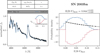 |
Fig. E.1. Spectral fits of SN 2003bn. See Fig. 6 for an explanation of the plot. |
| In the text | |
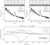 |
Fig. E.2. Spectral fits of SN 2006it. See Fig. 6 for an explanation of the plot. |
| In the text | |
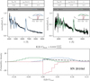 |
Fig. E.3. Spectral fits of SN 2010id. See Fig. 6 for an explanation of the plot. |
| In the text | |
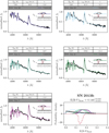 |
Fig. E.4. Spectral fits of SN 2013fs. See Fig. 6 for an explanation of the plot. |
| In the text | |
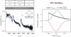 |
Fig. E.5. Spectral fits of SN 2019luo. See Fig. 6 for an explanation of the plot. |
| In the text | |
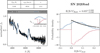 |
Fig. E.6. Spectral fits of SN 2020bad. See Fig. 6 for an explanation of the plot. |
| In the text | |
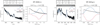 |
Fig. E.7. Spectral fits of SN 2020cvy and SN 2021gvv. See Fig. 6 for an explanation of the plot. |
| In the text | |
 |
Fig. E.8. Spectral fits of SN 2021hkf and SN 2021acvc. See Fig. 6 for an explanation of the plot. |
| In the text | |
Current usage metrics show cumulative count of Article Views (full-text article views including HTML views, PDF and ePub downloads, according to the available data) and Abstracts Views on Vision4Press platform.
Data correspond to usage on the plateform after 2015. The current usage metrics is available 48-96 hours after online publication and is updated daily on week days.
Initial download of the metrics may take a while.