| Issue |
A&A
Volume 702, October 2025
|
|
|---|---|---|
| Article Number | A58 | |
| Number of page(s) | 17 | |
| Section | Interstellar and circumstellar matter | |
| DOI | https://doi.org/10.1051/0004-6361/202553656 | |
| Published online | 07 October 2025 | |
Diffuse interstellar band λ6614 as a distance tracer for the Perseus, Taurus, and Orion molecular clouds: Feasibility and limitations
1
National Astronomical Observatories, Chinese Academy of Sciences,
Beijing
100101,
China
2
School of Astronomy and Space Science, University of Chinese Academy of Sciences,
Beijing
100049,
China
3
Purple Mountain Observatory and Key Laboratory of Radio Astronomy, Chinese Academy of Sciences,
10 Yuanhua Road,
Nanjing
210033,
PR China
★ Corresponding authors: This email address is being protected from spambots. You need JavaScript enabled to view it.
; This email address is being protected from spambots. You need JavaScript enabled to view it.
Received:
1
January
2025
Accepted:
22
July
2025
Abstract
Context. Diffuse interstellar bands (DIBs) are absorption features in the optical-to-near-infrared spectra of stars and they are associated with interstellar medium (ISM) carriers. They are valuable in studying the ISM, offering insights into its physical and chemical conditions, while tracing the distribution and kinematics of interstellar material.
Aims. We employed DIB λ6614 as a tracer to probe the distances and spatial distributions of interstellar material in the Perseus, Taurus, and Orion molecular clouds. These key star-forming regions in the solar neighborhood were analyzed to evaluate the feasibility and limitations of using DIB λ6614 as a tracer for distance and kinematic measurements.
Methods. We obtained stellar spectra from the Large Sky Area Multi-Object Fiber Spectroscopic Telescope medium-resolution survey within 600 pc. For hot stars (Teff ≥ 7500 K), DIB λ6614 was directly measured due to minimal contamination by stellar lines near the wavelength of 6614 Å. For cool stars (Teff < 7500 K), a template subtraction method was applied to isolate the ISM spectrum. Molecular cloud boundaries were identified based on 12CO emission maps integrated over velocity ranges, with 315, 684, 281, and 275 sources selected for Perseus, Taurus, Orion A, and Orion B, respectively.
Results. The DIB λ6614-derived distances to the molecular clouds are 297.2 ± 1.7 pc, 150.2 ± 1.2 pc, 421. 1 ± 0.7 pc, and 409.8 ± 0.7 pc for Perseus, Taurus, Orion A, and Orion B, respectively. These results are consistent with extinction-based distances, with discrepancies of 3–15 pc. In Perseus, two significant jumps in DIB λ6614 equivalent width are detected along the distance direction, with the first at ~152 pc, likely corresponding to the boundary of the Local Bubble.
Conclusions. DIB λ6614 is a robust tracer for molecular cloud distances, with estimates closely matching extinction-based measurements. DIB λ6614 is particularly effective for tracing diffuse regions and provides complementary insights into the structural details of molecular clouds.
Key words: ISM: clouds / dust, extinction
© The Authors 2025
 Open Access article, published by EDP Sciences, under the terms of the Creative Commons Attribution License (https://creativecommons.org/licenses/by/4.0), which permits unrestricted use, distribution, and reproduction in any medium, provided the original work is properly cited.
This article is published in open access under the Subscribe to Open model. This email address is being protected from spambots. You need JavaScript enabled to view it. to support open access publication.
1 Introduction
Diffuse interstellar bands (DIBs) are absorption features spanning optical to near-infrared (NIR) wavelengths. These features are observed in stellar spectra and are attributed to carriers in the interstellar medium (ISM, e.g., Jenniskens & Desert 1994). They were first recognized over a century ago by Heger (1922) as stationary lines at λλ5780 and 5797. Their interstellar origin was confirmed through later studies, including the detection of additional lines such as λλ6283 and 6614 (Merrill 1934). Although most of their carriers remain unidentified, the number of known DIBs has increased from the 39 cataloged in the seminal work by Herbig (1975) to more than 600 (Galazutdinov et al. 2017; Fan et al. 2019; McKinnon et al. 2024). DIBs have become invaluable tools for investigating the ISM due to their sensitivity to local environmental conditions and their ability to extract radial velocities (RVs) from their profiles (Zasowski et al. 2019). In particular, DIB λ6614 is correlated strongly with ISM properties such as extinction and neutral hydrogen column density (N(H)) (Friedman et al. 2011). These characteristics make it highly effective for tracing sightlines across the Galaxy and mapping large-scale Galactic structures, such as the Local Arm and the Perseus Arm. DIB λ6614 is also valuable for studying the spatial and kinematic distribution of interstellar material within molecular clouds (Istiqomah et al. 2020; Puspitarini & Lallement 2019; Ma et al. 2022).
In this work, we aim to evaluate the feasibility and limitations of DIBs as tracers for distances to three prominent star-forming regions in the solar neighborhood: the Perseus, Taurus, and Orion molecular clouds. These molecular clouds are ideal testbeds due to their proximity, minimal foreground contamination, and association with large-scale structures such as the Local Bubble (Leike et al. 2020). The Perseus molecular cloud, located at an average distance of ~300pc, spans approximately 7° × 3° on the sky and contains notable star-forming clusters, including IC 348 and NGC 1333 (Bally et al. 2008; Ortiz-León et al. 2018). The Taurus molecular cloud, at around 140 pc, spans approximately 15° × 12.5°, and it comprises one of the nearest regions of low-mass star formation (Dame et al. 1987, 2001; Luhman et al. 2010). The Orion molecular cloud complex, situated 400–500 pc away, includes extensively studied regions, such as Orion A and Orion B (Bally 2008). Several prior studies have mapped the distances and 3D structures of these molecular clouds. For instance, Schlafly et al. (2014) employed Pan-STARRS 1 (PS1) optical photometry to analyze stellar reddening along sightlines and estimate cloud distances. Additionally, Zucker et al. (2021) (hereafter, Z2l) integrated Gaia parallax measurements with dust extinction data from Leike et al. (2020), providing a comprehensive 3D structure and distance gradients for these clouds.
In the present study, we focus on DIB λ6614, which is correlated with key ISM properties and has been tested as a potential tracer of interstellar conditions. Tuairisg et al. (2000) measured the central wavelength (λc) of DIB λ6614 in air to be 6613.63 Å with a full width at half maximum (FWHM) of 1.14 Å based on high-resolution echelle spectrograph data. Fan et al. (2019) found a λc of 6613.74 Å, a FWHM of 1.05 Å, and a ratio of ΔEW/ΔE(B – V) = 185.14 mÅ mag−1 through APO survey data. Similarly, Vogrinčič et al. (2023) reported 6613.66 Å, a FWHM of 1.01 Å, and a ΔEW/ΔE(B – V) ratio of 130.37 mÅ mag−1 from GALAH survey data. Historically, DIB λ6614 was classified as a ζ-type DIB, indicating low-radiation, shielded environments (Cami et al. 1997; Moutou et al. 1999). However, recent studies, such as Fan et al. (2022), have reclassified it as a σ-type DIB associated with high-radiation, exposed environments, thereby demonstrating its broader relevance to diverse ISM conditions. This reclassification aligns with its observed behavior in molecular clouds, where DIB λ6614 exhibits broader spatial distributions compared to dust, potentially tracing diffuse regions that are less visible through traditional methods.
To obtain ISM spectra for cool stars, we applied a template matching method (Yuan & Liu 2012; Kos et al. 2013; Zhao et al. 2021; Ma et al. 2024). For hot stars, the DIB feature was measured directly. We also employed 12CO emission lines to identify regions within the three molecular clouds, subdividing them into more detailed sightlines. This approach allowed us to obtain precise distances to the molecular clouds, which were then compared with extinction data to refine our understanding of their structures.
The structure of this paper is as follows: in Sect. 2, we describe the spectral data used in this study. Section 3 details the methodology for measuring the DIB λ6614 feature and selecting regions within the Perseus, Taurus, and Orion molecular clouds. Section 4 presents the results of our analysis, followed by a discussion in Sect. 5. Finally, Sect. 6 provides a summary and conclusion of the study.
2 Data
The Large Sky Area Multi-Object Fiber Spectroscopic Telescope (LAMOST) is a reflective Schmidt telescope with a 4-meter effective aperture, a 5° field of view, and 4000 optical fibers, enabling simultaneous spectral observations of up to 4000 celestial objects over a 20-square-degree field (Zhao et al. 2012; Cui et al. 2012; Luo et al. 2015). Since 2018, LAMOST has been conducting the medium-resolution survey (MRS). This survey covers spectral ranges from 4950 to 5350 Å in the blue and from 6300 to 6800 Å in the red band, with a resolution of ~7500 (Wang et al. 2019; Liu et al. 2020). We used data from the LAMOST tenth data release (DR10) MRS, which covers spectral ranges that include prominent DIBs in the red band, such as λλ6379, 6614, 6660 (Wu et al. 2022). Among these, we selected the relatively strong DIB λ6614 as a tracer.
LAMOST DR10 has released a total of 10486 216 spectra1, offering a wealth of data for stellar and interstellar studies. However, the relatively narrow spectral coverage of LAMOST MRS data limits the accuracy of parameters derived from the default LAMOST Stellar Parameter Pipeline (LASP, Luo et al. 2015). Parameters such as effective temperature (Teff), surface gravity (log ɡ), and metallicity ([Fe/H]) are not precise enough for this study, impacting the quality of template matching and the accuracy of ISM spectrum extraction. To address these issues, previous studies such as Wang et al. (2020) (hereafter, W20), Xiang et al. (2022) (hereafter, X22), and Wang et al. (2023) (hereafter, W23) have provided refined stellar parameter measurements for LAMOST MRS spectra, ensuring the improved level of precision that is essential for this work.
We derived stellar parameters from the following sources. First, we matched our data with the stellar parameter catalog of W23, which offers Teff, log g, and [Fe/H] measurements for 1.38 million FGKM-type stars in LAMOST MRS DR8. The catalog provides accuracies of 76 K for Teff, 0.014 dex for log ɡ and 0.096 dex for [Fe/H] for stars with signal-to-noise ratio of S/N ≥ 10. This matching provided parameters for 631 405 stars. For stars missing in W23, we applied the SPCANet method from W20. This convolutional neural network (CNN) transfers stellar labels from high-resolution APOGEE-Payne data to LAMOST MRS spectra, achieving accuracies of 119 K for Teff and 0.17 dex for log g. This contributed valuable parameters for 327 177 stars. For hot stars, namely, OBA-type stars that were not available from the above sources, we relied on X22, which used LAMOST LRS DR6 spectra to estimate parameters for an additional 3449 stars. Finally, for stars unmatched by any of these methods, we relied on the LASP pipeline from LAMOST MRS DR10, which supplied parameters for 57 830 stars. Altogether, atmospheric parameters were determined for 1019 861 stars, meeting the requirements for reliable ISM spectrum extraction.
To refine our dataset further, we filtered the LAMOST MRS DR10 data to include stars with S/N ≥ 60 and distances ≤ 600 pc. Distances were determined as the median of photogeometric distances from the Gaia EDR3 catalog (Gaia Collaboration 2023), which combines parallax and photometry to provide more accurate estimates (Bailer-Jones et al. 2021). After filtering, the final dataset contained 552 442 spectra from 256 577 unique stars. For stars with repeated observations, we selected the spectrum with the highest S/N to maximize precision, minimizing uncertainties in detecting weak DIBs within the solar neighborhood. The distributions of stellar parameters (Teff, log ɡ, [Fe/H]) for the selected sample and the two-dimensional (2D) histogram of distance versus S/N are presented in Fig. 1.
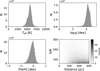 |
Fig. 1 Distributions of Teff, log ɡ, and [Fe/H] for the selected sample of 256 577 stars with S/N ≥ 60 and distances ≤600 pc from LAMOST MRS DR10. The bottom-right panel displays a 2D histogram of S/N versus distance. |
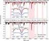 |
Fig. 2 Target and template absorption spectra for two stars. The pink shades indicate the masked regions for three DIBs (λλ6379, 6614, and 6660) as well as Hα when comparing the target spectrum and reference spectra. |
3 Method
3.1 Derive ISM spectra for hot and cool stars
The LAMOST data were originally in vacuum wavelengths and were converted to air wavelengths for consistency with previous research. For stars with Teff ≥ 7500 K, the spectra were directly treated as ISM spectra. To avoid the broad absorption feature of the Hα line, which has a central wavelength of 6562.79 Å in air2, we selected the 6604–6664 Å wavelength range for continuum normalization. The 60 Å band was processed by fitting the continuum with a third-order polynomial to account for the smoother absorption profiles typically observed in hot stars. Asymmetric sigma clipping was used in the continuum fitting. A 1σ threshold was applied below the continuum to exclude absorption features, and a more relaxed 3σ threshold was used above (as no prominent spectral lines were expected for that region) to suppress noise and outliers. The procedure was iterated 20 times to stabilize the continuum fitting (Zhao et al. 2021). Finally, the normalized ISM absorption spectrum was derived by dividing the observed spectrum by the fitted continuum.
For cool stars (Teff < 7500 K), the region near DIB λ6614 is increasingly affected by the blending of metallic absorption lines. To isolate the ISM features, we applied a template subtraction method to remove the stellar lines (Kos et al. 2013; Zhao et al. 2021; Ma et al. 2024). To select neighbor spectra with minimal or negligible ISM absorption features, we chose a total of 296 049 reference spectra. These were selected from stars with high Galactic latitude (|b| ≥ 30°), low extinction (E(B – V) ≤ 0.03, based on extinction values from Green et al. (2019)), and high S/N (S/N ≥ 30). Neighbor spectra were matched to target spectra based on stellar parameters within ∆Teff ≤ 100 K, ∆log ɡ ≤ 0.5 dex, and ∆[Fe/H] ≤ 0.2 dex. The selected neighbor spectra were normalized and ranked by S/N, with the top 50% retained for subsequent matching. After identifying suitable neighbor spectra, the 6300–6800 Å range was rebinned at 0.16 Å to ensure precise wavelength alignment. Due to the complex absorption features characteristic of cool stars, a fourth-order polynomial was applied for continuum normalization, differing from the third-order polynomial method used for hot stars. Neighbor spectra were ranked based on the difference metric D = Σ |(ƒtar – ƒtem)|, where ftar and ƒtem represent the normalized fluxes of the target and neighbor spectra, respectively. To minimize interference, regions around the Hα line (6540–6590 Å) as well as the DIBs λλ 6379 (6374–6384 Å), 6614 (6609–6619 Å), and 6660 (6655–6665 Å) were masked before calculating D. The top 25% of neighbor spectra with the smallest D values were then selected to form the final neighbor set. Subsequently, the selected neighbor spectra and the corresponding target spectrum were locally renormalized within the 6604–6664 Å range. The final template spectrum was obtained as the S/N-weighted average of the normalized fluxes of the selected neighbor spectra. The ISM spectrum was then derived by dividing the normalized target spectrum by the template spectrum. Figure 2 shows examples of two spectral subtraction templates, with red and black lines representing the target and template spectra, respectively.
 |
Fig. 3 Example of DIB λ6614 feature fitting for stars with different stellar parameters. The normalized ISM spectra are shown in black, with the DIB λ6614 feature modeled by a Gaussian profile in red. The blue vertical dashed line indicates the rest wavelength of DIB λ6614 in air at 6613.66 Å (Vogrinčič et al. 2023). The orange vertical dashed lines mark the wavelength range used for fitting. |
3.2 DIB λ6614 fit
The error for each pixel of the normalized ISM absorption spectrum was calculated as
 (1)
(1)
where ƒabS is the absorption flux and  is the inverse flux uncertainty provided by LAMOST. We assumed that the errors in the continuum flux follow a Poisson-like distribution. The error is defined as the root mean square (RMS) of the continuum, and ƒcont represents the fitted continuum. Gaussian profiles for the DIB λ6614 feature were fitted to the ISM spectra through a Markov chain Monte Carlo (MCMC) method, following Ma et al. (2024). The prior distribution was defined via
 (2)
(2)
Here, A, λc, and σ are the absorption depth, central wavelength, and Gaussian width, respectively. The likelihood distribution is expressed as
 (3)
(3)
where i represents each pixel in the spectrum. We employed an MCMC sampling to estimate the posterior distribution. The process initialized 100 walkers and conducted a burn-in of 100 steps followed by a production run of 1000 steps. The 16th, 50th, and 84th percentiles of the sample provided the best-fit parameters and uncertainties. Figure 3 shows examples of ISM spectra and their Gaussian fits.
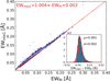 |
Fig. 4 Correlation between the integrated and fitted equivalent widths (EW6614) of the DIB λ6614 feature. The horizontal axis shows the fitted EW (EWfit), while the vertical axis displays the directly integrated EW (EWint). The histogram in the bottom-left corner shows the distribution of the difference ΔEW = EWint – EWfit. Here, µ and σ represent the mean and standard deviation of the ΔEW distribution, respectively. |
3.3 Measurement validation
To determine the presence of DIB λ6614, we calculated the equivalent width (EW) by integrating the spectrum over a µ±3σ range to obtain EWinte1. Additionally, we integrated over µ − 2 × 3σ to µ−3σ and µ + 3σ to µ + 2×3σ to calculate EWinte2· Here, µ and σ represent the central wavelength and width of the Gaussian profile fitted by MCMC. The presence of DIB 26614 was confirmed if EWinte1 > 2.5 × EWinte2. After filtering sources with Gaussian width (σ-6614) deviating by more than 3σ6614, we identified a total of 32 031 DIB 26614 detections. Figure 4 compares the EW values obtained from Gaussian fitting and direct integration. The results show a slope of 1.004, indicating close agreement between the two methods. The zoom-in panel in Fig. 4 shows the residual distribution between the integrated and fitted EW, with an average difference of 0.001, confirming the reliability of the Gaussian fitting for the DIB λ6614.
Figure 5 illustrates the 2D histogram distribution of σ6614 and λLSR6614. The mean σ6614 is measured to be 0.546 Å. After accounting for instrumental broadening using the method of Ma et al. (2024), this value remains consistent with the adjusted value of 0.57 Å reported by Vogrincic et al. (2023), based on their original measurement of 0.43 Å. Additionally, Fan et al. (2019) reported a σ6614 value of 0.45 Å, which was adjusted to 0.58 Å after accounting for instrumental broadening. To calculate λLSR6614 relative to the local standard of rest (LSR), we incorporated the solar motion values V⊙ = (U, V, W) = (10.6, 10.7, 7.6) km s−1 from Reid et al. (2019). The resulting λLSR6614 distribution shows a single peak centered at 6613.63 Å, corresponding to a VLSR6614 of approximately −1.36 km s−1, calculated using a rest wavelength of 6613.66 Å from Vogrincic et al. (2023).
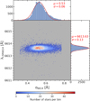 |
Fig. 5 Distribution of λLSR6614 as a function of σ6614. The central panel shows a 2D histogram of λLSR6614 versus σ6614, with color intensity indicating the number of stars per bin. The top and right marginal histograms display the distributions of σ6614 and λLSR6614, respectively, with Gaussian fits overlaid in red. The corresponding mean (µ) and standard deviation (σ) are indicated in each panel. |
3.4 Sample selection toward molecular clouds
Generally, 12CO is employed as an essential tracer for molecular clouds due to its observable rotational transitions, even in low-density molecular gas, making it a reliable indicator of H2 (Dame et al. 2001). To delineate the boundaries of the molecular clouds, we used Galaxy-wide CO data (WCO) from Dame et al. (2001). The data were integrated over velocity ranges of −10 to +20 km s−1 for all regions. These velocity ranges were explicitly defined by Lewis et al. (2022) and are illustrated in Fig. 6, which shows the WCO map encompassing the Perseus, Taurus, and Orion regions. Initially, contour values of 0.7 were used. However, the contours for Taurus and Perseus remained open and failed to form closed boundaries. To resolve this, we adjusted the contour levels to higher values, ensuring closed boundaries that better define the molecular clouds. Additionally, we incorporated molecular cloud spines from Zucker et al. (2021), depicted as gray points in Fig. 6, to guide the contour selection. For Perseus, we selected a contour value of 0.75, and for Taurus, we chose 0.95. These values allowed the contours to form closed boundaries, while maximizing the inclusion of the cloud spines. For Orion A and Orion B, although a contour value of 0.7 could form closed boundaries, we chose a value of 0.8 to better align with the spines identified by Zucker et al. (2021). This approach effectively captures core structures but may limit the spatial extent of identified clouds. We selected sources within the contours to represent internal cloud populations, totaling 315, 684, 281, and 275 sources for Perseus, Taurus, Orion A, and Orion B, respectively.
4 Results
4.1 Correlation with extinction
Figure 7 shows the relationship between EW6614 and interstellar extinction, represented by E(BP–RP), for the molecular clouds Perseus, Taurus, Orion A, and Orion B. The E(BP–RP) values were derived following the method in Zhao et al. (2024), which employs an XGBoost model to predict intrinsic colors ((BP – RP)0) based on Teff, log ɡ, and [M/H]. These stellar parameters are described in Sect. 2. Uncertainties were estimated by sampling atmospheric parameters from Gaussian distributions defined by their values and uncertainties. These samples were processed through the XGBoost model to compute the mean and standard deviation of the predicted (BP–RP)0. Observed BP and RP magnitudes, along with their measurement errors, were used to calculate observed colors (BP–RP). The extinction E(BP–RP) was obtained as the difference between observed and intrinsic colors. The total uncertainty was determined by propagating errors from both (BP–RP) and (BP–RP)0 estimates. As shown in Fig. 7, the errors in E(BP–RP) are small, but this does not account for errors from the XGBoost model. The upper panel of Fig. 7 shows the overall trend for all sources within 600 pc. The Pearson correlation coefficient is r = 0.70, with a slope of 0.134. In the lower panels, individual molecular clouds are analyzed. Perseus has a Pearson correlation coefficient of r = 0.64 and a slope of 0.07 based on 192 sources. Taurus shows r = 0.48 and a slope of 0.07 from 598 sources; Orion A shows r = 0.65 and a slope of 0.10 based on 33 sources; and Orion B has r = 0.60 with a slope of 0.09 based on 50 sources. The extinction ratio  for these regions was obtained from Zhang et al. (2023), with values of 3.22 for Perseus, 2.08 for Taurus, 3.36 for Orion A, and 3.23 for Orion B. Using the CCM89 extinction model from Cardelli et al. (1989), the
  ratios were determined to be 1.42, 1.39, 1.46, and 1.43 for the respective clouds. The corresponding
  values are 0.099, 0.097, 0.145, and 0.13 for Perseus, Taurus, Orion A, and Orion B, respectively. Across the aggregated sample within 600pc, assuming Rv = 3.1, we calculate
  . This analysis highlights a consistent positive correlation between EW6614 and interstellar extinction, both for individual molecular clouds and the full sample.
4.2 Distances to molecular clouds derived from DIB λ6614 and E(BP–RP)
The distances to molecular clouds are typically inferred by analyzing unreddened foreground stars and reddened back-ground stars through a star-by-star distance and reddening model (Schlafly et al. 2014; Zucker et al. 2019; Zhao et al. 2020). To estimate the distances to molecular clouds with the DIB λ6614, we adopted the formula in Eq. (2) from Ma et al. (2022), which models the variation of DIB λ6614 intensity or extinction with distance. In this work, we applied this formula as Eq. (4) to model the EW6614 jumps with distance across molecular clouds and to compare them to E(BP–RP), expressed as
 (4)
(4)
Here,  represents the amplitude of the jump in EW6614 or extinction at the cloud boundary; d0 is the central distance where the jump occurs; and δd defines the cloud size, corresponding to the cloud diameter derived from fitting the extinction or EW6614 data. Then,
  is the baseline level of EW6614 or extinction beyond the influence of the molecular cloud. The parameters in Eq. (4) were fitted by the MCMC method, capturing variations in EW6614 and extinction as a function of distance for stars within the four molecular clouds. We employed uniform priors for all four parameters. The constraints for the jump amplitude (
 ) were set to
  . For the central distance (d0), we used region-specific priors based on prior knowledge of approximate cloud locations: 100 < d0 < 200 pc for Taurus, 300 < d0 < 500 pc for Orion A and Orion B, and two separate ranges for Perseus to account for its complex structure: 100 < d0 < 200 pc for the foreground component and 200 < d0 < 400 pc for the main cloud. The cloud size parameter (δd) was constrained to 0 < δd < 50 pc, and the baseline level (
 ) was limited to
  . Posterior distributions for each parameter focused on the d0 and δd. Uncertainties were derived from the 16th and 84th percentiles, providing reliable estimates for the jump distance and size.
The results of these fits are shown in Fig. 8, where each panel corresponds to a specific molecular cloud. Table 1 summarizes the derived distances and sizes. Notably, an additional jump is observed in the foreground of the Perseus molecular cloud, where the EW6614 jump is more prominent compared to the one in E(BP–RP). The EW6614 jump occurs at approximately 152 pc with a size of 15 pc, while the E(BP–RP) jump is centered at 154 pc with a narrower size of 5 pc. The main DIB λ6614 jumps occur at distances of approximately 297 pc, 150 pc, 421 pc, and 410 pc for the Perseus, Taurus, Orion A, and Orion B molecular clouds, respectively, with corresponding sizes of 37 pc, 39 pc, 11 pc, and 18 pc. The E(BP-RP)-derived distances display a close match at 289 pc, 141 pc, 414 pc, and 406 pc, with slightly thinner sizes of 24 pc, 30 pc, 21 pc, and 19 pc, respectively. Across the four regions, the differences in distances derived from DIB λ6614 and E(BP–RP) remain within 15 pc, corresponding to a discrepancy of approximately 0–10%. In Fig. 9, we show the stacked spectra of the DIB λ6614 absorption feature across different distance intervals along the sightlines of the Perseus, Taurus, Orion A, and Orion B molecular clouds. Specifically for Perseus, the spectra were stacked before the first jump, between the first and second jumps, during the second jump, and after the second jump. The results clearly demonstrate that the DIB λ6614 absorption strength increases with distance, particularly at the first jump, indicating a genuine physical shift rather than a measurement artifact.
To further investigate the feasibility of DIB λ6614 as a tracer for the distances of molecular clouds, we analyzed pixelated sightlines toward the four molecular clouds, deriving distances based on EW6614 and E(BP–RP). The regions were divided using a HEALPix resolution of nside = 6 (0.92° per pixel) (Górski et al. 2005), ensuring an average of at least five sources per pixel (approximately 8–11 sources across the clouds). A finer resolution (nside = 7) resulted in too few sources per pixel for reliable analysis. Within each pixel, we examined variations of EW6614 and E(BP–RP) with distance. Pixels lacking sufficient data were merged with adjacent ones to ensure stable jump model fitting.
Studies by Z21 and Cao et al. (2023) (hereafter, C23) provide valuable benchmarks for evaluating the reliability of DIB λ6614 as a tool for measuring molecular cloud distances. Z21 utilized a 3D dust map constructed by Leike et al. (2020), which combined stellar reddening data with Gaia parallax measurements to create a spatially resolved extinction map. In contrast, C23 applied a star-by-star extinction approach, integrating observations from the LAMOST, Gaia, and 2MASS catalogs. Figure 10 presents the results of these pixelated distance measurements.
Each row corresponds to a different molecular cloud region, with the grayscale background representing WCO emission. The left panels show distances derived from Z21 extinction measurements. The middle and right panels depict pixelated distances derived from EW6614 and E(BP-RP), respectively, with the color scale indicating distance values. This visualization allows for a detailed comparison of the spatial distribution of distances obtained from different methods. Table C.1 presents the fitted DIB λ6614 and E(BP–RP) distances and sizes for the line-of-sight directions defined in this work, along with the corresponding results from Z21 and C23, although C23 provides fewer sightlines for the same directions.
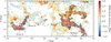 |
Fig. 6 12CO emission longitude-latitude map from Dame et al. (2001). The colors represent the 12CO velocity-integrated intensity on a logarithmic scale. Solid gray circles indicate the positions of molecular cloud spines identified by Zucker et al. (2021), which trace the central structures of the molecular clouds. Black contours correspond to a CO intensity of 0.7 (in logarithmic units), while blue contours represent different thresholds: 0.75 for Perseus, 0.95 for Taurus, and 0.8 for the Orion regions. |
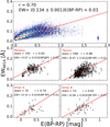 |
Fig. 7 Correlation between EW6614 and E(BP-RP). The top panel shows all sources within 600 pc. The middle and bottom panels focus on four molecular clouds: Perseus, Taurus, Orion A, and Orion B. Each sub-panel displays the linear fit for the respective cloud, along with the Pearson correlation coefficient, slope, and number of stars. Error bars indicate the uncertainties in EW6614 and E(BP-RP). A typical EW6614 uncertainty of 0.02 Å, represented by the black error bar, is shown in the bottom right corner of the top panel. |
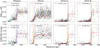 |
Fig. 8 EW6614 and E(BP–RP) as functions of distance for the Perseus, Taurus, Orion A, and Orion B regions. Gray dots represent stars with detected DIB λ6614. The red and cyan dashed curves show the fitted jumps using Eq. (4), with their central distances indicated in the legend of each subplot. The vertical blue dashed line marks the central distance of the jump, and the vertical orange dashed lines on either side outline the size of the cloud. |
Fitted cloud distances and sizes.
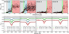 |
Fig. 9 Stacked spectra at different distances along the sightlines of the Perseus, Taurus, Orion A, and Orion B molecular clouds. The top panels correspond to Fig. 8, with shaded regions indicating distinct distance intervals. For Perseus, four intervals are defined: before the first intensity jump, between the first and second jumps, during the second jump, and beyond the second jump. For Taurus, the intervals are divided into four distance ranges: before the jump, during the jump, after the jump within 100 pc, and beyond up to 600 pc. For Orion A and Orion B, the distances are grouped into three intervals: before the jump, during the jump, and after the jump. The bottom panels show the stacked spectra of DIB λ6614 for each distance interval across the four molecular clouds, with error bars indicating the uncertainties in flux measurements. Each stacked spectrum displays a Gaussian fit to the DIB feature, with the EW6614 and σ6614 annotated. The color shading in the top panels corresponds to the colors of the stacked spectra in the bottom panels. |
4.3 Kinematics of DIB λ6614 and CO tracers in molecular clouds
To investigate the kinematic relationship between DIB λ6614 and molecular gas, Fig. 11 offers a comparison of the LSR velocities derived from DIB λ6614 measurements (VLSR6614; see Sect. 3.3) with those obtained from 12CO spectra ( ) across four star-forming regions: Perseus, Taurus, Orion A, and Orion B. The CO velocity statistics for each cloud are based on the median values along sightlines (Dame et al. 2001). For the Perseus cloud, the DIB λ6614 VLSR values were determined from sources located beyond the second jump, at distances exceeding 334 pc. For the Taurus cloud, only sources beyond the jump at distances over 189 pc were included.
In Table 2, we present a comparison of DIB λ6614 and CO kinematics across four molecular clouds, using three established rest wavelengths: 6613.56 Å (Galazutdinov et al. 2000), 6613.66 Å (Vogrinčič et al. 2023), and 6613.74 Å (Fan et al. 2019). The results show that the choice of rest wavelength significantly affects the derived velocity offsets between DIB and CO, with the ~ 0.2 Å variation leading to systematic shifts of up to ~ 8 km s−1. Such differences are sufficient to alter both the direction and magnitude of the apparent velocity discrepancy. These findings highlight the sensitivity of DIB λ6614 kinematics to rest wavelength uncertainties, which likely account for most of the observed differences relative to CO.
5 Discussion
The strength of DIBs shows a positive correlation with extinction, indicating that DIBs can effectively trace molecular clouds in a manner similar to extinction (Friedman et al. 2011). However, the absence of polarization in DIBs provides definitive evidence against dust grains as their carriers (Cox et al. 2011). The ratio of DIB strength to extinction appears to vary across different molecular clouds, as indicated by the differences in the linear fit slopes shown in Fig. 7, ranging from 0.07 ± 0.01 in Perseus to 0.10 ± 0.02 in Orion A. For the Perseus, Taurus, Orion A, and Orion B clouds, the  values are 0.099, 0.097, 0.145, and 0.13, respectively. These values are lower than the overall sample value of 0.188 within 600 pc and the value of 0.16 reported by Fan et al. (2019). The relatively higher ratios observed in Orion A and Orion B are consistent with the coefficient of 0.13 reported by Vogrinčič et al. (2023). However, these variations should be interpreted with caution, as some differences fall within the uncertainty margins. Given the limited data, these variations represent general trends rather than definitive correlations. A further analysis presented in Appendix B examines the distance dependence of this ratio, revealing significant regional variations. These results suggest that cloud properties and local ISM conditions may influence the ratio, highlighting the importance of further investigation to determine the physical mechanisms responsible for these variations.
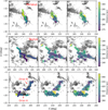 |
Fig. 10 Comparison of distance measurements for the Perseus, Taurus, Orion A, and Orion B molecular clouds. Each row corresponds to a different region in Galactic coordinates (ℓ, b). The grayscale background in all panels represents WCO emission. The left panels show distances derived from Z21 extinction measurements, displayed as continuous color maps. The middle and right panels show pixelated distance measurements derived from EW6614 and E(BP–RP), respectively, with the color scale indicating distance. An interactive display of the specific pixel-based jumps, as shown in Fig. 8, is available at https://zenodo.org/records/15294371 |
5.1 Comparison of molecular cloud distances and sizes derived from pixelated DIB λ6614 and E(BP–RP)
The distances derived from DIB λ6614 measurements in the pixelated analysis are generally consistent with those from E(BP–RP), Z21, and C23. For the Perseus molecular cloud, pixel-based DIB-derived distances range from 282 to 301 pc, with an average of 292 pc, in good agreement with E(BP–RP) (274–300 pc), Z21 (285–300pc), and C23 (285–306 pc). In Taurus, pixel-level DIB-derived distances span from 134 to 195 pc with an average of 157 pc, consistent with the E(BP–RP) range of 131–197 pc (average 152 pc). For Orion A, pixel-level DIB distances range from 402 to 444 pc (average 418 pc), closely matching the E(BP-RP) range (408–447 pc, average 417 pc). Similarly, in Orion B, pixel-based DIB distances (average 408 pc) demonstrate a strong agreement with E(BP–RP) (average 405 pc). This consistency confirms the effectiveness of DIB tracers as distance indicators.
The pixelated size estimates reveal systematic differences that highlight the complementary strengths of the two tracers. As shown in Fig. 12, DIB λ6614 generally yields largersizes than E(BP–RP) in pixel-based measurements, with 63% of sightlines exhibiting larger DIB-derived sizes and an average difference of 3.4 ± 0.9 pc. This offset reflects the ability of DIB λ6614 to trace diffuse outer envelopes of clouds that may be underrepresented in extinction-based measurements. Interestingly, although most sightlines in Orion A and B follow this trend, the overall cloud-scale fits in Table 1 show smaller DIB-derived sizes. This contrast likely arises because pixel-based analysis captures extended, diffuse structures along individual lines of sight, leading to larger size estimates, while global fits average over the entire cloud and are more influenced by compact, dense regions, which can result in smaller overall sizes. The histogram in Fig. 12 further reveals a bimodal distribution, featuring a main peak centered near 0 pc, indicating agreement between the two tracers, and a secondary peak around 7 pc, where DIB λ6614 systematically yields larger sizes. This pattern reinforces the role of DIBs in capturing the more extended and diffuse components of molecular clouds, which may be missed by extinction-based methods (Cox et al. 2024).
12CO and DIB 16614 velocities (in LSR) in clouds.
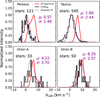 |
Fig. 11 Comparison of VLSR for DIB λ6614 and 12CO spectra across four molecular cloud regions. The black stepped lines show the histogram of DIB 16614 velocities in the LSR frame, while the red lines represent the normalized12 CO spectra. The purple dashed lines show the Gaussian fits to the DIB 16614 velocity distributions for each cloud. The mean velocities (µ) and standard deviations (σ) are annotated in each panel. The number of stars used for each region is also indicated. |
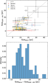 |
Fig. 12 Comparison of the cloud sizes of sub-regions in the four molecular clouds as traced by DIB λ6614 and E(BP–RP). The upper panel presents the correlation between size estimates derived from DIB λ6614 and E(BP–RP), with error bars representing measurement uncertainties and colors indicating different molecular clouds. The gray dashed line marks the 1:1 relation. The lower panel shows the distribution of the differences between the two sets of size estimates. |
5.2 Challenges in interpreting structural gradients with DIB λ6614 tracer
While DIB-derived distances generally align with other methods, interpreting structural gradients within molecular clouds remains challenging. In Perseus, both E(BP-RP) and Z21 data reveal a gradient, with distances decreasing from IC 348 to NGC 1333. DIB-derived distances follow a similar pattern, with IC 348 at 298 pc and NGC 1333 at 289 pc. However, due to measurement uncertainties and the broader distribution of DIB carriers, the gradient is less clearly defined in the DIB data. In Taurus, a distinct north-to-south gradient is observed in the E(BP–RP) data. For instance, in the northern region (D1–L1544), the DIB-derived distance of 177 pc slightly the exceeds E(BP–RP) distance of 175 pc and Zucker’s estimate of 172 pc (Zucker et al. 2022), likely reflecting the presence of extended outer cloud layers. In contrast, the southern region (D3–South; ℓ = 176.48°, b = −18.08°) exhibits a decrease in distances across all methods, with values of 134 pc for DIB λ6614, 136 pc for E(BP–RP), and 122 pc for Z21. This trend suggests a denser structure located closer to the observer. In Orion A and Orion B, the DIB-derived distances are largely consistent with those from E(BP–RP) and Z21. However, at the cloud edges (e.g., ℓ = 214.38°, b = −17.65°), both tracers report larger distances, likely due to reduced extinction and the diffuse nature of the outer regions.
5.3 Implications for distance tracing: cloud and local structures
Focusing on the Perseus molecular cloud, the first significant DIB jump at approximately 152.1 pc offers key insights into the physical structure of the cloud. As illustrated in Fig. 9, this jump corresponds to a sharp increase in EW6614, suggesting a transition from a lower-density to a higher-density region within the ISM. We hypothesize that this first jump corresponds to the shell of the Local Bubble rather than an internal structure of the Perseus cloud. To test this hypothesis, we refer to Pelgrims et al. (2020), who mapped the Local Bubble shell along different sightlines. According to their results, the shell in the direction of Perseus lies between approximately 107.5 pc and 113.9 pc. However, the observed DIB jump at ~152.1 pc indicates a discrepancy of roughly 50 pc. Interestingly, this distance aligns with the dust map from Edenhofer et al. (2024), which shows extinction increasing near 140–150 pc toward Perseus. This suggests that the DIB jump may trace the same structure as the dust. The discrepancy with Pelgrims’ estimate may indicate that the Local Bubble’s shell in this direction may be fragmented or extended rather than uniform. Further observations of the ISM are required to determine whether this feature indeed corresponds to the boundary of the Local Bubble or represents a different interstellar transition. These results demonstrate the potential of DIB λ6614 as a complementary tracer for molecular cloud distances and interstellar structures.
Unlike traditional extinction-based methods, DIBs offer independent insight into diffuse ISM variations. Our findings show that DIBs consistently validate extinction-based distances, while offering enhanced sensitivity to diffuse, low-extinction structures. Future observations of other DIBs, such as λ6379 and λ6660, using LAMOST MRS across broader samples, will refine the utility of DIBs as tracers and to further delineate the boundaries of large-scale ISM features such as the Local Bubble.
6 Conclusions
We selected the Perseus, Taurus, and Orion molecular clouds to evaluate the feasibility of using DIB λ6614 as a tracer for molecular cloud distances, based on spectra from the LAM-OST MRS DR10 survey. The strength of DIB λ6614 shows a positive correlation with interstellar extinction, although the correlation coefficients vary among different clouds. By fitting EW6614 as a function of distance with an error function, we identified the jump center as the estimated distance to the molecular cloud. The DIB-derived distances closely match those from extinction-based methods, with discrepancies ranging from 3 to 15 pc.
A more detailed analysis of the sightlines indicates that DIB-derived jump distances generally display a good agreement with extinction measurements. However, the majority of DIB-based jumps exhibit broader sizes than their extinction-derived counterparts. A kinematic comparison of VLSR values from DIB λ6614 and 12CO reveals differences that are influenced not only by measurement uncertainties, but also by the choice of rest wavelength for DIB λ6614. We find that the rest wavelength of 6613.56 Å results in the smallest difference between the VLSR of the DIB λ6614 and that of CO.
In conclusion, DIB λ6614 is shown to be a reliable tracer of molecular cloud distances that complements extinction-based approaches. While the diffuse nature of DIBs may limit their precision in denser regions, they remain effective, extinction-independent tracers of the ISM, offering unique insights that complement extinction-based ISM maps. Future studies incorporating additional DIB features (e.g., λ6379, λ6660) and higher-resolution spectroscopy will further improve the reliability and application of DIBs in mapping the ISM and molecular cloud structures.
Data availability
The data underlying this article are available from the LAM-OST MRS DR10 dataset, which can be accessed at http://www.lamost.org/dr10/v1.0/. This includes all spectra analyzed for the DIB λ6614 features across the selected sightlines in the Perseus, Taurus, and Orion molecular clouds. For further inquiries regarding the dataset, users are encouraged to consult the LAMOST Data Release documentation available on the website. Additionally, distance measurements and sizes along sightlines in the Perseus, Taurus, Orion A, and Orion B molecular clouds can be accessed via https://zenodo.org/records/15294371
Acknowledgements
This work is supported by National Natural Science Foundation of China (grant Nos. 12090044) and National Key R&D Program of China (Grant NO. 2019YFA0405102). Guoshoujing Telescope (the Large Sky Area Multi-Object Fiber Spectroscopic Telescope, LAMOST) is a National Major Scientific Project built by the Chinese Academy of Sciences. Funding for the Project has been provided by the National Development and Reform Commission. LAMOST is operated and managed by the National Astronomical Observatories, Chinese Academy of Sciences. H.Z. acknowledges the National Natural Science Foundation of China (grant No. 12203099) and the China Postdoctoral Science Foundation (No. 2022M723373). We thank the reviewers for their valuable comments and suggestions that helped improve this manuscript. Software: Astropy (Astropy Collaboration 2013; Astropy Collaboration 2018; Astropy Collaboration 2022), TOPCAT (Taylor 2005), emcee (https://emcee.readthedocs.io/en/stable/), uncertainties (https://uncertainties-python-package.readthedocs.io/en/latest/index.html), healpy (https://healpy.readthedocs.io/en/latest/index.html).
Appendix A EW and RV measurement errors for cool and hot stars
The EW is calculated as  , where A represents the DIB depth and σ is the width. The associated errors are propagated from the MCMC-fitted uncertainties in A and σ. The number of spectra with detected DIBs is 31 282 for cool stars and 673 for hot stars. As shown in Fig. A.1, the measurement errors for cool stars are generally larger than those for hot stars, in both EW and VLSR. The mean EW error for cool stars is 0.014, compared to 0.009 for hot stars, while the mean VLSR error for cool stars is 4.337 km s−1, higher than the 2.863 km s−1 observed for hot stars. This discrepancy likely arises because the spectra of cool stars are not directly measured, but instead reconstructed by subtracting a stellar template spectrum in order to isolate the interstellar absorption features. This process may reduce the S/N of the ISM spectra, increasing measurement uncertainties and leading to larger errors for the cool star spectra compared to those of hot stars.
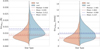 |
Fig. A.1 Violin plot distribution of EW6614 and |

Appendix B Dependence of the DIB λ6614-to-dust ratio on distance and local environment
To investigate the environmental dependence of the ratio between DIB λ6614 and dust extinction, we analyze all samples within 600 pc using consistent distance bins of 50 pc. Figure B.1 presents the variation of  with distance for different regions, excluding bins containing fewer than ten sources. For the complete sample, the ratio increases systematically from approximately 0.05 at 125 pc to about 0.13 at 575 pc, with an increase around 200 pc that likely corresponds to the edge of the Local Bubble. Within the Local Bubble, the low ratio may reflect a reduced abundance or excitation efficiency of DIB 26614 carriers in the low-density, high-temperature environment, consistent with its classification as a ζ-type DIB.
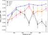 |
Fig. B.1 Variation in the |

In Perseus, the ratio increases to a maximum of ~0.09 at 225 pc, then decreases beyond 250 pc, reaching near-zero or even negative values in some bins. Beyond 300 pc, the DIB-to-dust ratio becomes very noisy and difficult to constrain properly, likely resulting from the combination of low dust extinction in those lines of sight—where extinction does not increase with distance—and the relative abundance of DIB λ6614 carriers. This effect is also seen in Taurus, where the ratio peaks around 375 pc before declining. Despite these variations, the overall trends broadly follow the behavior of the full sample. Due to limited detection of DIB λ6614 within 400 pc in the Orion region, the ratio can only be reliably calculated for distance bins beyond that range. The specific fitted values and the number of sources in each distance bin are summarized in Table B.1. While no definitive conclusions can be drawn from these observations, they suggest that the DIB λ6614-to-extinction ratio is sensitive to both distance and local cloud environment. Nevertheless, Fig. B.1 still captures the signature of the Local Bubble.
Distance-binned  for Perseus, Taurus, Orion, and all sources.
Appendix C Distances along different sightlines
Distances and sizes along sightlines in the Perseus, Taurus, Orion A, and Orion B molecular cloudsc.
References
- Astropy Collaboration (Robitaille, T. P., et al.) 2013, A&A, 558, A33 [NASA ADS] [CrossRef] [EDP Sciences] [Google Scholar]
- Astropy Collaboration (Price-Whelan, A. M., et al.) 2018, AJ, 156, 123 [Google Scholar]
- Astropy Collaboration (Price-Whelan, A. M., et al.) 2022, ApJ, 935, 167 [NASA ADS] [CrossRef] [Google Scholar]
- Bailer-Jones, C. A. L., Rybizki, J., Fouesneau, M., Demleitner, M., & Andrae, R. 2021, AJ, 161, 147 [Google Scholar]
- Bally, J. 2008, in Handbook of Star Forming Regions, ed. B. Reipurth (USA: ASP Monograph), 1, 459 [NASA ADS] [Google Scholar]
- Bally, J., Walawender, J., Johnstone, D., Kirk, H., & Goodman, A. 2008, in Hand-book of Star Forming Regions, ed. B. Reipurth (USA: ASP Monograph), 1, 308 [Google Scholar]
- Cami, J., Sonnentrucker, P., Ehrenfreund, P., & Foing, B. H. 1997, A&A, 326, 822 [NASA ADS] [Google Scholar]
- Cao, Z., Jiang, B., Zhao, H., & Sun, M. 2023, ApJ, 945, 132 [NASA ADS] [CrossRef] [Google Scholar]
- Cardelli, J. A., Clayton, G. C., & Mathis, J. S. 1989, ApJ, 345, 245 [Google Scholar]
- Cox, N. L. J., Ehrenfreund, P., Foing, B. H., et al. 2011, A&A, 531, A25 [NASA ADS] [CrossRef] [EDP Sciences] [Google Scholar]
- Cox, N. L. J., Vergely, J. L., & Lallement, R. 2024, A&A, 689, A38 [NASA ADS] [CrossRef] [EDP Sciences] [Google Scholar]
- Cui, X.-Q., Zhao, Y.-H., Chu, Y.-Q., et al. 2012, Res. Astron. Astrophys., 12, 1197 [Google Scholar]
- Dame, T. M., Ungerechts, H., Cohen, R. S., et al. 1987, ApJ, 322, 706 [NASA ADS] [CrossRef] [Google Scholar]
- Dame, T. M., Hartmann, D., & Thaddeus, P. 2001, ApJ, 547, 792 [Google Scholar]
- Edenhofer, G., Zucker, C., Frank, P., et al. 2024, A&A, 685, A82 [NASA ADS] [CrossRef] [EDP Sciences] [Google Scholar]
- Fan, H., Hobbs, L. M., Dahlstrom, J. A., et al. 2019, ApJ, 878, 151 [NASA ADS] [CrossRef] [Google Scholar]
- Fan, H., Schwartz, M., Farhang, A., et al. 2022, MNRAS, 510, 3546 [NASA ADS] [CrossRef] [Google Scholar]
- Friedman, S. D., York, D. G., McCall, B. J., et al. 2011, ApJ, 727, 33 [NASA ADS] [CrossRef] [Google Scholar]
- Gaia Collaboration (Vallenari, A., et al.) 2023, A&A, 674, A1 [NASA ADS] [CrossRef] [EDP Sciences] [Google Scholar]
- Galazutdinov, G. A., Musaev, F. A., Krelowski, J., & Walker, G. A. H. 2000, PASP, 112, 648 [NASA ADS] [CrossRef] [Google Scholar]
- Galazutdinov, G. A., Lee, J.-J., Han, I., et al. 2017, MNRAS, 467, 3099 [NASA ADS] [CrossRef] [Google Scholar]
- Górski, K. M., Hivon, E., Banday, A. J., et al. 2005, ApJ, 622, 759 [Google Scholar]
- Green, G. M., Schlafly, E., Zucker, C., Speagle, J. S., & Finkbeiner, D. 2019, ApJ, 887, 93 [NASA ADS] [CrossRef] [Google Scholar]
- Heger, M. L. 1922, Lick Observ. Bull., 10, 146 [Google Scholar]
- Herbig, G. H. 1975, ApJ, 196, 129 [NASA ADS] [CrossRef] [Google Scholar]
- Istiqomah, A. N., Puspitarini, L., & Arifyanto, M. I. 2020, J. Phys. Conf. Ser., 1523, 012009 [NASA ADS] [CrossRef] [Google Scholar]
- Jenniskens, P., & Desert, F. X. 1994, A&AS, 106, 39 [NASA ADS] [Google Scholar]
- Kos, J., Zwitter, T., Grebel, E. K., et al. 2013, ApJ, 778, 86 [NASA ADS] [CrossRef] [Google Scholar]
- Leike, R. H., Glatzle, M., & Enßlin, T. A. 2020, A&A, 639, A138 [NASA ADS] [CrossRef] [EDP Sciences] [Google Scholar]
- Lewis, J. A., Lada, C. J., & Dame, T. M. 2022, ApJ, 931, 9 [NASA ADS] [CrossRef] [Google Scholar]
- Liu, C., Fu, J., Shi, J., et al. 2020, arXiv e-prints [arXiv:2005.07210] [Google Scholar]
- Luhman, K. L., Allen, P. R., Espaillat, C., Hartmann, L., & Calvet, N. 2010, ApJS, 186, 111 [Google Scholar]
- Luo, A. L., Zhao, Y.-H., Zhao, G., et al. 2015, Res. Astron. Astrophys., 15, 1095 [Google Scholar]
- Ma, W.-J., Chen, J.-J., Li, Y.-B., et al. 2022, MNRAS, 511, 3708 [Google Scholar]
- Ma, X.-X., Chen, J.-J., Luo, A. L., et al. 2024, A&A, 691, A282 [NASA ADS] [CrossRef] [EDP Sciences] [Google Scholar]
- McKinnon, K. A., Ness, M. K., Rockosi, C. M., & Guhathakurta, P. 2024, ApJ, 965, 120 [Google Scholar]
- Merrill, P. W. 1934, PASP, 46, 206 [NASA ADS] [CrossRef] [Google Scholar]
- Moutou, C., Krelowski, J., D’Hendecourt, L., & Jamroszczak, J. 1999, A&A, 351, 680 [NASA ADS] [Google Scholar]
- Ortiz-León, G. N., Loinard, L., Dzib, S. A., et al. 2018, ApJ, 865, 73 [Google Scholar]
- Pelgrims, V., Ferrière, K., Boulanger, F., Lallement, R., & Montier, L. 2020, A&A, 636, A17 [EDP Sciences] [Google Scholar]
- Puspitarini, L., & Lallement, R. 2019, J. Phys. Conf. Ser., 1245, 012027 [Google Scholar]
- Reid, M. J., Menten, K. M., Brunthaler, A., et al. 2019, ApJ, 885, 131 [Google Scholar]
- Schlafly, E. F., Green, G., Finkbeiner, D. P., et al. 2014, ApJ, 786, 29 [NASA ADS] [CrossRef] [Google Scholar]
- Taylor, M. B. 2005, ASP Conf. Ser., 347, 29 [Google Scholar]
- Tuairisg, S. Ó., Cami, J., Foing, B. H., Sonnentrucker, P., & Ehrenfreund, P. 2000, A&AS, 142, 225 [NASA ADS] [CrossRef] [EDP Sciences] [Google Scholar]
- Vogrinčič, R., Kos, J., Zwitter, T., et al. 2023, MNRAS, 521, 3727 [NASA ADS] [CrossRef] [Google Scholar]
- Wang, R., Luo, A. L., Chen, J. J., et al. 2019, ApJS, 244, 27 [NASA ADS] [CrossRef] [Google Scholar]
- Wang, R., Luo, A. L., Chen, J.-J., et al. 2020, ApJ, 891, 23 [Google Scholar]
- Wang, R., Luo, A. L., Zhang, S., et al. 2023, ApJS, 266, 40 [NASA ADS] [CrossRef] [Google Scholar]
- Wu, K.-F., Luo, A. L., Chen, J.-J., Hou, W., & Zhao, Y.-H. 2022, Res. Astron. Astrophys., 22, 085007 [Google Scholar]
- Xiang, M., Rix, H.-W., Ting, Y.-S., et al. 2022, A&A, 662, A66 [NASA ADS] [CrossRef] [EDP Sciences] [Google Scholar]
- Yuan, H., & Liu, X. 2012, MNRAS, 425, 425 [Google Scholar]
- Zasowski, G., Finkbeiner, D. P., Green, G. M., et al. 2019, BAAS, 51, 314 [NASA ADS] [Google Scholar]
- Zhang, R., Yuan, H., & Chen, B. 2023, ApJS, 269, 6 [NASA ADS] [CrossRef] [Google Scholar]
- Zhao, G., Zhao, Y.-H., Chu, Y.-Q., Jing, Y.-P., & Deng, L.-C. 2012, Res. Astron. Astrophys., 12, 723 [NASA ADS] [CrossRef] [Google Scholar]
- Zhao, H., Jiang, B., Li, J., et al. 2020, ApJ, 891, 137 [CrossRef] [Google Scholar]
- Zhao, H., Schultheis, M., Recio-Blanco, A., et al. 2021, A&A, 645, A14 [NASA ADS] [CrossRef] [EDP Sciences] [Google Scholar]
- Zhao, H., Wang, S., Jiang, B., et al. 2024, ApJ, 974, 138 [Google Scholar]
- Zucker, C., Speagle, J. S., Schlafly, E. F., et al. 2019, ApJ, 879, 125 [NASA ADS] [CrossRef] [Google Scholar]
- Zucker, C., Goodman, A., Alves, J., et al. 2021, ApJ, 919, 35 [NASA ADS] [CrossRef] [Google Scholar]
- Zucker, C., Goodman, A. A., Alves, J., et al. 2022, Nature, 601, 601 [Google Scholar]
All Tables
Distances and sizes along sightlines in the Perseus, Taurus, Orion A, and Orion B molecular cloudsc.
All Figures
|
Fig. 1 Distributions of Teff, log ɡ, and [Fe/H] for the selected sample of 256 577 stars with S/N ≥ 60 and distances ≤600 pc from LAMOST MRS DR10. The bottom-right panel displays a 2D histogram of S/N versus distance. |
| In the text | |
|
Fig. 2 Target and template absorption spectra for two stars. The pink shades indicate the masked regions for three DIBs (λλ6379, 6614, and 6660) as well as Hα when comparing the target spectrum and reference spectra. |
| In the text | |
|
Fig. 3 Example of DIB λ6614 feature fitting for stars with different stellar parameters. The normalized ISM spectra are shown in black, with the DIB λ6614 feature modeled by a Gaussian profile in red. The blue vertical dashed line indicates the rest wavelength of DIB λ6614 in air at 6613.66 Å (Vogrinčič et al. 2023). The orange vertical dashed lines mark the wavelength range used for fitting. |
| In the text | |
|
Fig. 4 Correlation between the integrated and fitted equivalent widths (EW6614) of the DIB λ6614 feature. The horizontal axis shows the fitted EW (EWfit), while the vertical axis displays the directly integrated EW (EWint). The histogram in the bottom-left corner shows the distribution of the difference ΔEW = EWint – EWfit. Here, µ and σ represent the mean and standard deviation of the ΔEW distribution, respectively. |
| In the text | |
|
Fig. 5 Distribution of λLSR6614 as a function of σ6614. The central panel shows a 2D histogram of λLSR6614 versus σ6614, with color intensity indicating the number of stars per bin. The top and right marginal histograms display the distributions of σ6614 and λLSR6614, respectively, with Gaussian fits overlaid in red. The corresponding mean (µ) and standard deviation (σ) are indicated in each panel. |
| In the text | |
|
Fig. 6 12CO emission longitude-latitude map from Dame et al. (2001). The colors represent the 12CO velocity-integrated intensity on a logarithmic scale. Solid gray circles indicate the positions of molecular cloud spines identified by Zucker et al. (2021), which trace the central structures of the molecular clouds. Black contours correspond to a CO intensity of 0.7 (in logarithmic units), while blue contours represent different thresholds: 0.75 for Perseus, 0.95 for Taurus, and 0.8 for the Orion regions. |
| In the text | |
|
Fig. 7 Correlation between EW6614 and E(BP-RP). The top panel shows all sources within 600 pc. The middle and bottom panels focus on four molecular clouds: Perseus, Taurus, Orion A, and Orion B. Each sub-panel displays the linear fit for the respective cloud, along with the Pearson correlation coefficient, slope, and number of stars. Error bars indicate the uncertainties in EW6614 and E(BP-RP). A typical EW6614 uncertainty of 0.02 Å, represented by the black error bar, is shown in the bottom right corner of the top panel. |
| In the text | |
|
Fig. 8 EW6614 and E(BP–RP) as functions of distance for the Perseus, Taurus, Orion A, and Orion B regions. Gray dots represent stars with detected DIB λ6614. The red and cyan dashed curves show the fitted jumps using Eq. (4), with their central distances indicated in the legend of each subplot. The vertical blue dashed line marks the central distance of the jump, and the vertical orange dashed lines on either side outline the size of the cloud. |
| In the text | |
|
Fig. 9 Stacked spectra at different distances along the sightlines of the Perseus, Taurus, Orion A, and Orion B molecular clouds. The top panels correspond to Fig. 8, with shaded regions indicating distinct distance intervals. For Perseus, four intervals are defined: before the first intensity jump, between the first and second jumps, during the second jump, and beyond the second jump. For Taurus, the intervals are divided into four distance ranges: before the jump, during the jump, after the jump within 100 pc, and beyond up to 600 pc. For Orion A and Orion B, the distances are grouped into three intervals: before the jump, during the jump, and after the jump. The bottom panels show the stacked spectra of DIB λ6614 for each distance interval across the four molecular clouds, with error bars indicating the uncertainties in flux measurements. Each stacked spectrum displays a Gaussian fit to the DIB feature, with the EW6614 and σ6614 annotated. The color shading in the top panels corresponds to the colors of the stacked spectra in the bottom panels. |
| In the text | |
|
Fig. 10 Comparison of distance measurements for the Perseus, Taurus, Orion A, and Orion B molecular clouds. Each row corresponds to a different region in Galactic coordinates (ℓ, b). The grayscale background in all panels represents WCO emission. The left panels show distances derived from Z21 extinction measurements, displayed as continuous color maps. The middle and right panels show pixelated distance measurements derived from EW6614 and E(BP–RP), respectively, with the color scale indicating distance. An interactive display of the specific pixel-based jumps, as shown in Fig. 8, is available at https://zenodo.org/records/15294371 |
| In the text | |
|
Fig. 11 Comparison of VLSR for DIB λ6614 and 12CO spectra across four molecular cloud regions. The black stepped lines show the histogram of DIB 16614 velocities in the LSR frame, while the red lines represent the normalized12 CO spectra. The purple dashed lines show the Gaussian fits to the DIB 16614 velocity distributions for each cloud. The mean velocities (µ) and standard deviations (σ) are annotated in each panel. The number of stars used for each region is also indicated. |
| In the text | |
|
Fig. 12 Comparison of the cloud sizes of sub-regions in the four molecular clouds as traced by DIB λ6614 and E(BP–RP). The upper panel presents the correlation between size estimates derived from DIB λ6614 and E(BP–RP), with error bars representing measurement uncertainties and colors indicating different molecular clouds. The gray dashed line marks the 1:1 relation. The lower panel shows the distribution of the differences between the two sets of size estimates. |
| In the text | |
|
Fig. A.1 Violin plot distribution of EW6614 and |
| In the text | |
|
Fig. B.1 Variation in the |
| In the text | |
Current usage metrics show cumulative count of Article Views (full-text article views including HTML views, PDF and ePub downloads, according to the available data) and Abstracts Views on Vision4Press platform.
Data correspond to usage on the plateform after 2015. The current usage metrics is available 48-96 hours after online publication and is updated daily on week days.
Initial download of the metrics may take a while.