| Issue |
A&A
Volume 702, October 2025
|
|
|---|---|---|
| Article Number | A163 | |
| Number of page(s) | 29 | |
| Section | Extragalactic astronomy | |
| DOI | https://doi.org/10.1051/0004-6361/202553828 | |
| Published online | 17 October 2025 | |
Tracing the galaxy-halo connection with galaxy clustering in COSMOS-Web from z = 0.1 to z ∼ 12
1
Institut d’Astrophysique de Paris, UMR 7095, CNRS, Sorbonne Université, 98 bis boulevard Arago, F-75014 Paris, France
2
Cosmic Dawn Center (DAWN), Denmark
3
Niels Bohr Institute, University of Copenhagen, Jagtvej 128, 2200 Copenhagen, Denmark
4
Aix Marseille University, CNRS, CNES, LAM, Marseille, France
5
Department of Astronomy, The University of Texas at Austin, 2515 Speedway Blvd Stop C1400, Austin, TX 78712, USA
6
Purple Mountain Observatory, Chinese Academy of Sciences, 10 Yuanhua Road, Nanjing 210023, China
7
Department of Astronomy and Astrophysics, University of California, Santa Cruz, 1156 High Street, Santa Cruz, CA 95064, USA
8
Department of Physics and Astronomy, University of Hawaii, Hilo, 200 W Kawili St, Hilo, HI 96720, USA
9
Jet Propulsion Laboratory, California Institute of Technology, 4800 Oak Grove Drive, Pasadena, CA 91109, USA
10
Laboratory for Multiwavelength Astrophysics, School of Physics and Astronomy, Rochester Institute of Technology, 84 Lomb Memorial Drive, Rochester, NY 14623, USA
11
Space Telescope Science Institute, 3700 San Martin Drive, Baltimore, MD 21218, USA
12
Caltech/IPAC, 1200 E. California Blvd., Pasadena, CA 91125, USA
13
Northeastern University, 100 Forsyth St., Boston, MA 02115, USA
14
NASA Goddard Space Flight Center, Code 662, Greenbelt, MD 20771, USA
15
Université de Strasbourg, CNRS, Observatoire astronomique de Strasbourg, UMR 7550, 67000 Strasbourg, France
16
Department of Astrophysical Sciences, Princeton University, Princeton, NJ 08544, USA
17
LUX, Observatoire de Paris, Université PSL, Sorbonne Université, CNRS, 75014 Paris, France
18
Department of Astronomy, University of Massachusetts, Amherst, MA 01003, USA
⋆ Corresponding author: This email address is being protected from spambots. You need JavaScript enabled to view it.
Received:
20
January
2025
Accepted:
1
August
2025
Abstract
We explore the evolving relationship between galaxies and their dark matter halos from z ∼ 0.1 to z ∼ 12 using mass-limited angular clustering measurements in the 0.54 deg2 of the COSMOS-Web survey, the largest contiguous JWST extragalactic survey. This study provides the first measurements of the mass-limited two-point correlation function at z ≥ 10 and a consistent analysis spanning 13.4 Gyr of cosmic history, setting new benchmarks for future simulations and models. Using a halo occupation distribution (HOD) framework, we derived characteristic halo masses and the stellar-to-halo mass ratio (SHMR) across redshifts and stellar mass bins. Our results first indicate that HOD models fit data at z ≥ 2.5 best when incorporating a nonlinear scale-dependent halo bias, boosting clustering at nonlinear scales (r = 10 − 100 kpc). We find that galaxies at z ≥ 10.5 with log(M⋆/M⊙)≥8.85 are predominantly central galaxies in halos with Mh ∼ 1010.5 M⊙, achieving a star formation efficiency (SFE) of εSF = M⋆/(fbMh) up to 1 dex higher than at z ≤ 1. The high galaxy bias at z ≥ 8 suggests that these galaxies reside in massive halos with an intrinsic high SFE, challenging stochastic SHMR scenarios. Our SHMR evolves significantly with redshift, starting very high at z ≥ 10.5, decreasing until z ∼ 2 − 3, then increasing again until the present. Current hydrodynamical simulations fail to reproduce both massive high-z galaxies and this evolution, while semi-empirical models linking SFE to halo mass, accretion rates, and redshift align with our findings. We propose that early galaxies (z > 8) experience bursty star formation without significant feedback altering their growth, driving the rapid growth of massive galaxies observed by JWST. Over time, the increasing feedback efficiency and the exponential halo growth end up suppressing star formation. At z ∼ 2 − 3 and later, the halo growth slows down, while star formation continues, supported by gas reservoirs in halos.
Key words: galaxies: evolution / galaxies: halos / galaxies: high-redshift / galaxies: statistics
© The Authors 2025
 Open Access article, published by EDP Sciences, under the terms of the Creative Commons Attribution License (https://creativecommons.org/licenses/by/4.0), which permits unrestricted use, distribution, and reproduction in any medium, provided the original work is properly cited.
This article is published in open access under the Subscribe to Open model. This email address is being protected from spambots. You need JavaScript enabled to view it. to support open access publication.
1. Introduction
The important role played by dark matter in the formation and evolution of galaxies is broadly acknowledged. In the classic White & Rees (1978) paradigm, galaxies form at the center of dark matter halos. Dark matter shapes the distribution of galaxies on large scales (Davis et al. 1985) and this large-scale environment plays a key role in the galaxy assembly process. Thus, to improve our understanding of galaxy formation and evolution over cosmic time, it is crucial to explore the connection between galaxies and their dark matter halos (see Wechsler & Tinker 2018 for a review). The halo mass influences the efficiency of gas cooling, which is essential for the formation of galaxies (White & Frenk 1991). Additionally, processes regulating star formation, such as mergers (Lacey & Cole 1993), feedback mechanisms (e.g., supernovae feedback in low-mass halos, and feedback from active galactic nuclei in high-mass halos; see Bower et al. 2006), gas accretion rates (e.g., Conroy & Wechsler 2009), or galaxy dynamics (e.g., Rodriguez-Gomez et al. 2017) are also likely influenced by halo mass.
Estimating the mass of dark matter halos hosting galaxies is therefore crucial. While direct methods like weak gravitational lensing can measure halo masses, they are typically limited to low redshifts due to the need for well-resolved sources. Indirect methods, such as abundance matching and clustering, can be applied over a larger range in redshift. Clustering measures the spatial distribution of galaxies using the two-point autocorrelation function, which quantifies the excess of galaxy pairs relative to a random distribution. By comparing how galaxies are clustered to the clustering of halos of different masses, we can infer the typical halo mass hosting them. Galaxy clustering studies began in the 1970s when simple power-law models were fitted to correlation functions measured using catalogs derived by photographic plates (Totsuji & Kihara 1969; Groth & Peebles 1977; Peebles 1980). These works laid the foundation for modern approaches, which now use the halo occupation distribution (HOD) framework (Peacock & Smith 2000; Cooray & Sheth 2002; Smith et al. 2003). HOD models, derived for stellar mass-selected samples, provide a powerful tool for estimating halo masses and other properties by assuming a halo model that populates halos of a certain mass with central and satellite galaxies. Asgari et al. (2023) recently published a review of the halo model formalism.
With these models, clustering analyses have offered significant insights into the galaxy-halo connection, mostly constraining its evolution at z ≤ 3. The James Webb Space Telescope (JWST) has now opened a new observational window reaching back to z ≥ 10, revealing the first galaxies formed in the Universe (e.g., Finkelstein et al. 2022; Naidu et al. 2022b; Curtis-Lake et al. 2023; Carniani et al. 2024; Kokorev et al. 2025). Early observations indicate an overabundance ofmassive, bright galaxies at z ≥ 10 compared to predictions (e.g., in COSMOS, Casey et al. 2024; Shuntov et al. 2025b; Franco et al. 2024); massive quiescent galaxies at z ≥ 4 (e.g., Carnall et al. 2024; Weibel et al. 2025); or red, compact sources with active galactic nuclei (AGN) emission (e.g., Labbé et al. 2023; Greene et al. 2024; Matthee et al. 2024). Such discoveries challenge predictions of stellar mass assembly in hierarchical models of structure formation and raise new questions about the relationship between galaxies and their halos during these epochs, as theoretical models struggle to reproduce these observations. These challenges extend to hydrodynamical simulations, which are calibrated on low-redshift data and face inherent limitations due to resolution and volume. Small-box, high-resolution simulations such as SPHINX (Katz et al. 2023) and OBELISK (Trebitsch et al. 2021) provide insights into the formation of low-mass galaxies at high z, but lack the large-scale coverage needed to study global trends, while large-volume simulations like TNG (Pillepich et al. 2018; Nelson et al. 2018; Marinacci et al. 2018; Naiman et al. 2018; Springel et al. 2018) and HORIZON-AGN (Dubois et al. 2014) are less reliable in capturing the detailed baryonic processes at play during the reionization era. As a result, key aspects of the galaxy-halo connection, including the evolution of the stellar-to-halo mass ratio (SHMR) and star formation efficiency, are still not fully settled at z > 3.
Recent JWST studies have focused on one-point statistics, such as the ultraviolet (UV) luminosity function (UVLF; e.g., Finkelstein et al. 2023; Harikane et al. 2023; Finkelstein et al. 2024; Chemerynska et al. 2024) and the stellar mass function (SMF; e.g., Navarro-Carrera et al. 2024; Weibel et al. 2024; Shuntov et al. 2025b), which are important quantities for understanding galaxy properties. However, these measurements can suffer from degeneracies, depending on the assumptions made about galaxy evolution such as star formation histories, dust attenuation, or its connection with large-scale structures (e.g., Muñoz et al. 2023 and Gelli et al. 2024 have discussed the importance of galaxy bias in this context). While one-point statistics provide useful constraints, two-point statistics such as galaxy clustering offer more detailed information, allowing for the mapping of high-z galaxies to their halos and large-scale environments. High-z clustering studies have used UV magnitudes (e.g., Dalmasso et al. 2024b for samples at z ∼ 8; Dalmasso et al. 2024a for z ∼ 11), but these samples are often incomplete, as is also the case with Lyman-break galaxy samples at z ∼ 5 − 8 (Ouchi et al. 2004; Lee et al. 2006; Overzier et al. 2006; Hatfield et al. 2018; Barone-Nugent et al. 2014). While stellar masses become less reliable at high z due to the increasing uncertainties on the assumptions mentioned above, they do offer complementary insights. In contrast to UV magnitudes, these data provide a cumulative view of galaxy growth and are less sensitive to bursty star formation activity. Furthermore, the small fields used in these JWST studies are prone to biases due to cosmic variance, which may affect the results and limit our understanding of the broader galaxy population (Ucci et al. 2021; Steinhardt et al. 2021; Jespersen et al. 2025).
In this study, we use the COSMOS-Web survey (Casey et al. 2023), the largest contiguous extragalactic survey observed with JWST to date. We investigate the galaxy–halo connection from the Local Universe to z ∼ 12 using photometric redshifts in COSMOS-Web. Spanning an area of 0.54 deg2, this survey reduces cosmic variance, enabling us to probe a wide range of densities and large-scale environments. We performed a consistent angular galaxy clustering analysis from z = 0.1 to z > 10, using stellar mass-limited, complete samples. By applying HOD models, we were able to extract characteristic halo masses and study the SHMR across this broad redshift range, gaining insights into the star formation efficiency in the early Universe and its evolution through cosmic time.
This paper is organized as follows. In Sect. 2, we begin with a description of the COSMOS-Web observations and catalogs, along with a discussion of how we construct a mass-complete galaxy sample. Section 3 presents the theory used to model galaxy clustering measurements using the HOD formalism. In Sect. 4, we present the galaxy clustering measurements and their corresponding fits, comparing our findings with the literature and examining the evolution of best-fit parameters such as the characteristic halo masses and the SHMR. We set these results into a broader context and discuss their implications for the galaxy-halo connection from cosmic dawn to the Local Universe in Sect. 5. Finally, Sect. 6 summarizes and concludes our analysis. Throughout this work, we adopted the AB magnitudes (Oke & Gunn 1983) and cosmology from Planck Collaboration VI (2020). Stellar masses are computed assuming a Chabrier (2003) initial mass function (IMF).
2. Observations
2.1. The COSMOS-Web survey and catalogs
COSMOS-Web (Casey et al. 2023, GO#1727, PI: Casey & Kartaltepe) is a JWST survey that covers a contiguous area of 0.54 deg2 in the COSMOS field in four NIRCam filters (F115W, F150W, F277W, F444W). Imaging from one MIRI filter, F770W, is also provided over a non-contiguous area of 0.19 deg2. These images reach a 5σ depth1 of about 28.1 mag in the F444W band and 25.2 in F770W. Details on the NIRCam and MIRI image processing are presented in Franco et al. (2025b) and Harish et al. (2025). Here, we use the complete COSMOS-Web NIRCam survey area, observed at three dates (January 2023, April 2023, and January 2024), along with observations from April 2024 that completed visits missed in earlier epochs due to issues such as guide star failures. This work uses the “COSMOS2025” catalog constructed by combining the COSMOS-Web JWST data with the rich multiwavelength coverage already present in COSMOS (Shuntov et al. 2025a). A brief overview of the 37 imaging bands available in this catalog can be found below:
-
Near-UV imaging with the u-band from the Canada-France-Hawaii Telescope (CFHT) Large Area u-band Deep Survey (CLAUDS; Sawicki et al. 2019);
-
Ground-based optical imaging from the Hyper Suprime-Cam (HSC) Subaru Strategic Program third data release, with broad bands g, r, i, z, y, and three narrow bands (Aihara et al. 2018b, 2022);
-
Images from the Subaru Suprime-Cam with 12 medium bands in the optical between 4266 Å and 8243 Å (Taniguchi et al. 2007, 2015);
-
Near-infrared (NIR) imaging, including ground-based data from the final “legacy” data release (DR6) of the UltraVista survey (McCracken et al. 2012; Milvang-Jensen et al. 2013), comprising four broad bands Y, J, H, Ks, and one narrow band at 1.18 μm;
-
Space-based optical imaging with Hubble Space Telescope (HST) from the Advanced Camera for Surveys (ACS) F814W band (Koekemoer et al. 2007).
The object detection followed a “hot-cold” strategy, using SEP (Barbary 2016; python implementation of SExtractor, Bertin & Arnouts 1996), applied to a combined  image of all NIRCam bands (e.g., Szalay et al. 1999). First, the “cold” mode detects and deblends bright and extended sources with a shallow threshold. Next, a second “hot” mode run is performed on the same image from which the bright sources were masked, to detect faint, isolated sources and push the detection to fainter magnitudes. We note that this detection image covers only the 0.5 deg2 COSMOS-Web area, unlike the UltraVISTA-selected “COSMOS2020” catalog, which covers approximately 1.5 deg2 of the COSMOS area (Weaver et al. 2022). However, NIRCam data are much deeper than UltraVISTA, allowing us to reach considerably lower stellar mass and higher redshift limits than in COSMOS2020.
The 37-band COSMOS-Web photometry is extracted using a new model fitting version of SExtractor, SourceXtractor++ (Kümmel et al. 2020; Bertin et al. 2020). The main advantage of this package is that there is no longer a need to resample input images to equivalent pixel scales (which would certainly be problematic for combining 0.030″ NIRCam images with the 0.15″ dataset used in COSMOS2020). Instead, morphological profiles can be fitted for each source across images with different resolutions and sensitivities. For each object, a Sérsic model (Sérsic 1963) convolved with the point spread function (PSF) is fitted on all NIRCam bands simultaneously. Then the fluxes and magnitudes in each band are extracted based on these fitted morphological parameters. To minimize photometric errors caused by blending, overlapping sources are grouped and fitted together. Full details about COSMOS-Web catalogs can be found in Shuntov et al. (2025a).
The photometric redshifts (photo-z) and physical parameters are determined using LePHARE (Arnouts et al. 2002; Ilbert et al. 2006). This tool fits galaxy spectral energy distribution (SED) templates generated from stellar population models from the Bruzual & Charlot (2003) library and a diverse set of star formation histories, as detailed in Ilbert et al. (2015). It includes star and quasi-stellar object (QSO) templates. LePHARE additionally: 1) incorporates the effects of dust attenuation by adjusting the color excess E(B − V) from 0 to 1.2, considering three attenuation curves (Calzetti et al. 2000; Arnouts et al. 2013; Salim et al. 2018); (2) accounts for emission lines (following a method similar to Schaerer & de Barros 2009); and 3) adds the intergalactic medium absorption through the analytical correction of Madau (1995). After a marginalization over templates and dust laws, a redshift likelihood distribution is returned and physical parameters are subsequently derived at the fixed redshift. The photo-z and stellar mass estimates for each object are then provided as the medians of the resulting probability density functions, hereafter referred to as PDF(z), with a 1σ confidence interval given by the 16th and 84th percentiles. The photo-z accuracy is then assessed by comparing to a compilation of about 12 000 spectroscopic redshifts (spec-z) up to z = 8 from various programs in COSMOS, which is presented in Khostovan et al. (2025). The precision is quantified by
 (1)
(1)
with Δz = zphot − zspec. It achieves values better than 0.015 for galaxies in the magnitude range 23 < mF444W < 25. For fainter galaxies at 25 < mF444W < 28, the precision σMAD remains below 0.030, with an outlier fraction lower than 10% (outliers are defined by |Δz|> 0.15 [1 + zspec]).
2.2. Sample selection
2.2.1. Completeness
To reliably measure galaxy clustering with the added ability to interpret these results, we must first be certain that our catalog contains representative samples of the parent galaxy populations. We started with a careful cleaning of the sample. We removed objects classified as stars in LePHARE, based on their better χ2 fit to star or brown dwarf SED templates, along with a compactness criterion. We also excluded objects with a radius smaller than twice the full-width-at-half-maximum (FWHM) in the F115W image and those flagged as hot pixels or other image artifacts. Moreover, we masked the region around bright stars in the NIRCam images: objects contained inside it are excluded from the analysis (representing ∼2% of the total population). The same masking technique was applied to the optical images, specifically based on HSC stars that are very bright. This last procedure resulted in the removal of ∼15% of the objects from the initial catalog.
We considered our sample incomplete if fainter than the magnitude limit of mF444Wlim = 27.75. This value was derived from the number counts completeness of the survey compared to a deeper JWST survey in the same field, PRIMER-COSMOS, covering a common area of ∼200 arcmin2 (following the same method as Shuntov et al. 2025b, which also gives more details on PRIMER-COSMOS). These galaxy counts are shown in Fig. 1 for both surveys with a fitted power law in the range 23 ≤ mF444W ≤ 27. The bottom panel shows their magnitude completeness, defined respectively as the ratio of the number counts in COSMOS-Web over PRIMER-COSMOS and as the number counts in PRIMER-COSMOS over the power law fit. We chose the magnitude cut when the COSMOS-Web completeness drops below 80% (corresponding to mF444Wlim = 27.75).
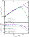 |
Fig. 1. Top: Galaxy number counts for COSMOS-Web and PRIMER-COSMOS, along with a fitted power law in the range 23.0 ≤ mF444W ≤ 27.0 (dashed line). Errors are computed according to Poisson noise only. Bottom: Magnitude completeness for COSMOS-Web and PRIMER-COSMOS, defined respectively as the ratio of number counts in COSMOS-Web over PRIMER-COSMOS and as the number counts in PRIMER-COSMOS over the fitted power law. The dotted black line shows the magnitude cut for COSMOS-Web where completeness falls to 80%, used for this work. |
Finally, to select stellar mass thresholds for our clustering measurements, we needed to compute the completeness of the galaxies according to stellar mass. We used the empirical method from Pozzetti et al. (2010): for each galaxy in a given redshift bin, one determines the mass at which it can be observed at the magnitude limit in a chosen band. Here, we chose the reddest NIRCam filter F444W, which probes the post-Balmer break region where the emission from older stars dominates at z > 3, along with the limit magnitude computed above. This leads to the following formula:
 (2)
(2)
which estimates the mass M⋆lim that a galaxy with stellar mass M⋆ and F444W magnitude mF444W would have if it was observed at mF444Wlim. The stellar mass completeness is then defined as the M⋆lim within which 90% of galaxies lie. Figure 2 shows the stellar mass of galaxies as a function of their photometric redshift, along with COSMOS-Web and COSMOS2020 (from Weaver et al. 2022) stellar mass completeness curves. Thanks to the much deeper COSMOS-Web NIRCam observations, mass limits are approximately one order of magnitude lower than COSMOS2020, allowing us to probe lower-mass and higher-redshift galaxies.
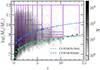 |
Fig. 2. Stellar mass distribution as a function of redshift of COSMOS-Web sources, with the mass completeness limits for COSMOS-Web in green (with errors calculated as the M⋆lim values that correspond to 85 or 95% of galaxies) and COSMOS2020 in blue as given in Weaver et al. (2022). All galaxies after magnitude filtering only are shown. Redshift bins and stellar mass thresholds, used for clustering measurements, are also represented in solid purple lines. |
2.2.2. High-redshift selection
Since the beginning of JWST observations, several high-redshift candidates identified using photometric redshifts have, in fact, turned out to be heavily dust-obscured, lower-redshift galaxies (e.g., Naidu et al. 2022a; Zavala et al. 2023; Fujimoto et al. 2023). To remove these interlopers from our clustering sample at high z, we performed a more advanced cleaning for the redshift bins at z ≥ 4.
First, we identified that a significant fraction of sources selected initially in the high-z sample were actually hot pixels (image artifacts). These objects are flagged in the catalog using a method based on size and compactness, as described in Shuntov et al. (2025a), and were excluded from the sample across all redshift bins.
Secondly, some z ≥ 4 sources are found to be better fitted by a QSO template at lower redshifts, likely due to an AGN-dominated emission. Such sources can mimic high-redshift galaxies, falsifying photo-z and stellar mass estimates because LePHARE does not distinguish between stellar and AGN components in the SED. This is also particularly true for AGN-dominated objects with significant dust obscuration (e.g., little red dots, LRDs; Matthee et al. 2024). To exclude AGN-dominated contaminants, we applied criteria based on their spectral and morphological properties, following the methodology of Shuntov et al. (2025b) and Akins et al. (2025). Specifically, we removed sources at z ≥ 4 that are (I) compact, with an effective radius Reff < 0.1″ (FWHM of F277W’s PSF) and a flux ratio in F444W between two apertures as 0.5 < F(0.2″)/F(0.5″) < 0.7; and (II) either with a better AGN SED fit with χAGN2 < χGAL2; or red with mF277W − mF444W > 1.5 indicating AGN emission in the rest-frame optical. To summarize, the criterion is ((AGN ∪ red) ∩ compact).
At higher redshifts, we found that assumptions in the SED fitting code, such as the amount of dust attenuation or emission lines allowed, can significantly impact photo-z estimates at high redshift. For instance, some high-z candidates shift to low z if we increase the covered range in E(B − V). Examining specific objects, we observed that using the redshift at maximum likelihood (denoted zchi2) might be more reliable than the median of the probability density function (denoted zPDF) employed in this work (Sect. 2.1). A comparison between zPDF and zchi2 is shown in Appendix A. Discrepancies between these two estimates arise because zchi2 corresponds to the redshift of the template that minimizes the χ2, which may be the only model at that redshift, while zPDF represents the median of the summed probabilities from all templates at a given redshift, making it generally more robust. However, we consider that the limited variety of templates at high z, due to the relatively recent observation of early galaxies and the current lack of well-established SED models for these populations, can excessively bias the PDF toward low-z solutions, even when the best-fit template corresponds to a higher redshift. Therefore, for the 8 ≤ z < 10.5 and 10.5 ≤ z < 14 bins, we considered galaxies with either zPDF or zchi2 within the bin. To refine the sample and remove obvious low-z sources, we applied additional cleaning criteria as below.
-
Signal-to-noise ratio (S/N) criteria: sources must have S/N(F277W) ≥2 and S/N(F444W) ≥2 as the Lyman break for z < 14 is expected in bluer wavelengths.
-
Neighboring redshift bins: for galaxies selected based only on zchi2, we exclude those having their zPDF and zchi2 close (satisfying |zPDF − zchi2|≤3), but with a zPDF that falls outside the redshift bin of interest, typically in an adjacent z bin. We consider these objects to be more likely true intermediate-z galaxies identified by zPDF rather than low-z interlopers incorrectly assigned to high redshift. They are then included in the appropriate previous redshift bins.
-
Detection in optical bands: we ran the package photutils on optical cutouts from HST, HSC, and a stack of HSC bands to perform the source detection. We also added F115W for galaxies at z ≥ 10.5 as their Lyman-break falls after this band. Galaxies with a ≥2σ detection were removed.
-
Visual inspection: we manually inspected all cutouts and SED fits left of z ≥ 8 sources to remove image artifacts, incorrectly deblended sources, or false detections.
Figure 3 shows the evolution of galaxy number counts in these high-z bins after each cleaning step. These steps removed from 5 to 20% of sources selected by zchi2, while those selected by zPDF appear more robust. This led to 715 and 26 galaxies having with both zPDF and zchi2 in the bin, 30 and 11 galaxies with only zPDF, and 377 and 182 galaxies with only zchi2, for the 8 ≤ z < 10.5 and 10.5 ≤ z < 14 bins, respectively. From this, we defined two final samples for our work: the “conservative sample” that includes zPDF-selected galaxies only (so 715 + 30 sources for the 8 ≤ z < 10.5 bin, and 26 + 11 at 10.5 ≤ z < 14); and the “extended sample” which adds to the conservative one zchi2-selected galaxies. Since zPDF is more conservative as it accounts for all templates over redshift, we adopted it as the correct redshift estimate for the other low redshift bins, making the selection of the so-called high-z conservative sample consistent with low-z bins.
 |
Fig. 3. Numbers of galaxies in our two highest redshift bins after the different cleaning steps applied one after the other. The top bar (dark colors) represents galaxies selected by zPDF and the bottom bar (light colors) by zchi2. |
This search for a better completeness does not come without risk of contamination, however. To illustrate this, we stacked PDF(z) distributions for galaxies having both photo-z in the bin versus only one: see Fig. 4. When both are in the bin, the stacked PDF(z) shows a strong peak in the high-z bin with a smaller counterpart at lower z. For galaxies with only zPDF in the bin, we see a strong high-z peak and a narrower low-z peak where zchi2 lies. Conversely, for those with only zchi2 in the bin, the probability density spans z = 0 to 5, with a small bump in the high-z bin. At z ≥ 10.5, we see the contribution from the two main low-z interloper populations: one at z ∼ 3 − 5, corresponding to strong emission-line galaxies or dusty star-forming galaxies that boost NIRCam photometry and mimic a blue continuum slope (Naidu et al. 2022a; Zavala et al. 2023), and another at z ∼ 1, caused by massive dusty galaxies with Balmer breaks falling into the NIR bands, mimicking the Lyman break and combined with dust reddening.
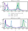 |
Fig. 4. Stack of PDF(z) in our two highest redshift bins for galaxies selected by zPDF and/or zchi2. Thin lines indicate stacks of 15 galaxies and solid lines are stacks of 50 galaxies. |
To further test the contamination of our samples, we computed the cross-correlations of mass-limited samples between distinct redshift bins (presented in Appendix C). We compare it to the autocorrelations (shown in Sect. 3.1), finding that the ratio between the two becomes particularly lower at z ≥ 3. At lower redshifts, the autocorrelation is, on average (across all scales), 1 to 2 dex higher than the cross-correlation. However, at 3 ≤ z < 8, this ratio drops below 1 dex for several cross-correlations with low-z bins. While we did not expect zero cross-correlations due to the magnification bias, this effect cannot account for the signal we observe as it is expected to be as w(θ) < 10−2 (e.g., Hildebrandt et al. 2009; Xu et al. 2023). The trend becomes even more pronounced when considering more massive galaxies. At the highest redshifts (z ≥ 8), the ratio continues to decrease, with the autocorrelation being only about three times higher than the cross-correlation, on average.
Hence, the sample at z ≥ 10 remains uncertain. This is combined with the fact that these sources are only constrained by two or three photometric bands. While the absence of detections in bluer bands supports their high-redshift nature, the lack of data leads to poorly constrained SED fits and, consequently, more uncertain stellar mass estimates. We therefore advise interpreting the z ≥ 10 results with caution, as they remain preliminary measurements subject to sample contamination. A more detailed inspection of z ≥ 10 sources in COSMOS-Web is presented in Franco et al. (2025a).
2.2.3. Redshift – stellar mass binning and distributions
We measured galaxy clustering and number densities in stellar mass- and volume-limited samples. Mass thresholds were determined starting from the stellar mass completeness limit and were then arbitrarily set to achieve a sufficient number of galaxies for clustering analysis. Additionally, redshift width bins were defined by hand to ensure a roughly similar number of galaxies in each bin up to z ∼ 4, facilitating comparisons. For z ≥ 4, we chose bins in such a way to ensure that there are at least 100 galaxies in each bin at the end of the cleaning process. This is a limit determined empirically to ensure enough statistics for measuring clustering. These bins are illustrated in Fig. 2, and the corresponding numbers of galaxies in each redshift-mass bin after cleaning are detailed in Appendix B.
We excluded objects from bins at z < 8 if their PDF(z) has more than 70% of its distribution outside the range z ± Δzbin, where Δzbin is the width of the redshift bin of interest. This criterion removes objects with poorly constrained PDF(z), often contaminants or unlikely to belong to the redshift bin. Approximately 20% of objects were removed per bin, but we confirmed that changes in clustering measurements remain within the error bars after this exclusion. Ultimately, the final dataset used for this work comprised a total of ∼240 000 galaxies above the completeness limits.
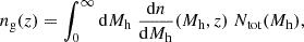
Furthermore, modeling the angular correlation function requires accurate redshift distributions, noted N(z). We used the method derived in Euclid Collaboration: Ilbert et al. (2021), which takes advantage of photo-z likelihoods returned by SED fitting codes such as LePHARE. For each redshift and stellar mass selected sample, N(z) can be estimated by stacking individual posterior probabilities, 𝒫(z|o), for a galaxy inside the bin to have a redshift, z, considering a color (in the full covered wavelength range, noted c) and magnitude (in a reference band, noted m0) vector, o = (c, m0). This posterior, by marginalizing over NSED templates, can be written as the product of the photo-z likelihood, ℒ(o|z), and a prior probability of z given a reference magnitude Pr(z|m0, i), expressed as
 (3)
(3)
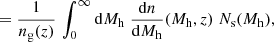
Euclid Collaboration: Ilbert et al. (2021) showed that an appropriate prior would be as below, calculated within magnitude bins centered at m0,
 (4)
(4)
where Θ(m0, i|m0) = 1 if the object magnitude m0, i is within the magnitude bin, and 0 otherwise. The authors show that this prior can have a significant impact on the median redshift estimate, quantified as μ(δz)∼0.01(1 + z) for an Euclid configuration. This bias could be due to the SED fitting directly (not adapted templates, degeneracies, etc.), a non-adequate photo-z prior, or more. They propose a correction that is however not applicable to COSMOS-Web currently because this technique assumes overestimated photo-z uncertainties and a training set of spec-z representing all galaxy populations in the sample. Nonetheless, Shuntov et al. (2022) showed that for the COSMOS2020 catalog, this bias could lead to differences in the clustering of the order of 3%, which is below the error bars associated with our clustering measurements.
An example of resulting redshift distributions for all galaxies above the stellar mass completeness limit for each redshift bin in our study is shown in Fig. 5. The sharp peaks in some distributions likely result from large-scale structures in the survey area; for example some of these peaks at z < 3 are confirmed by the COSMOS spec-z compilation (Khostovan et al. 2025). Alternatively, they may arise from LePHARE fitting technique, where the code can converge on a narrow range of values when it gets stuck in local minima, particularly when handling low S/N sources. We can see in the 10.5 < z < 14 redshift distribution the contributions from SED solutions corresponding to galaxies at z ∼ 1 and z ∼ 3 − 5, as discussed in Sect. 2.2.2.
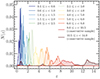 |
Fig. 5. Redshift distributions for galaxies above the stellar mass completeness limit in the redshift bins chosen for this work. |
3. Measurements and modeling
3.1. Galaxy clustering measurements
In this work, we computed the angular correlation function (ACF) w(θ) between galaxy positions separated by an angle θ via the Landy & Szalay (1993) estimator. It involves comparing the observed galaxy catalog with a randomly distributed one:
 (5)
(5)
Here, for each angular bin [θ, θ + δθ], DD is the number of galaxy pairs in the observed catalog, RR the number of pairs in a random catalog and DR between both catalogs. This random catalog was created using the code venice2. It is based on the exact same area of the survey (after applying HSC and JWST masked regions, Sect. 2.2.1) and composed of ∼50 times the total number of objects in the survey. We measured the ACF using the package TreeCorr3 (Jarvis et al. 2004), across a range of angular scales determined to be above the resolution and above the total area of the survey: 10−5 ≤ θ ≤ 10−1 deg, with a number of theta bins Nθ ∈ [10, 15].
Statistical errors associated with the ACF were determined using the jackknife resampling method implemented in TreeCorr. The entire area was divided in Npatches = 20 sub-samples of ∼90 arcmin2 each (except for the two highest-z bins where we reduced Npatches to 9 and 7, respectively), and the ACF was computed by excluding one patch at a time. This yielded a covariance matrix expressed as
![Mathematical equation: $$ \begin{aligned} C_{ij} = \frac{N_{\rm patches}-1}{N_{\rm patches}} \sum _{k=1}^{N_{\rm patches}} \left[ w_k(\theta _i) - \overline{w}(\theta _i) \right]^T \, \left[ w_k(\theta _j) - \overline{w}(\theta _j) \right], \, \end{aligned} $$](/articles/aa/full_html/2025/10/aa53828-25/aa53828-25-eq7.gif) (6)
(6)
where  is the mean ACF and wk the estimate of w(θ) when the k-th patch is excluded. This allows us to address Poisson noise in the count of galaxy pairs and cosmic variance at large angular scales arising from the finite survey area. However, it is important to note that uncertainties due to cosmic variance may still be underestimated as the patches cannot be fully independent and some correlated large-scale structures might contaminate the covariance of the data.
Although COSMOS-Web is one of the largest surveys observed by JWST, its spatial coverage is still limited. This can bias clustering measurements, particularly at large scales, where the amplitude may be underestimated. This effect is called the “integral constraint” bias (IC; Groth & Peebles 1977) and a constant correction factor wIC can be expressed in terms of survey area, Ω:
 (7)
(7)
Roche & Eales (1999) proposed to use the random catalog to compute this term as a function of the “true” ACF, wtrue,
 (8)
(8)
where wtrue(θ) = wmes(θ)+wIC. In our case, we applied this factor only to the model ACF wmod, true(θ) before fitting and not directly to the measurements, according to wmod(θ) = wmod, true(θ)−wIC(wmod, true, RR). Its impact becomes significant at scales above 0.02 deg and reaches up to one order of magnitude at the largest scales.
Finally, we also computed the number density of galaxies,  , for each sample, in each redshift–mass bin. This is defined as the number of galaxies, Ng, in a sample limited by the stellar mass threshold, M⋆,th, divided by the comoving volume V probed by the redshift bin, [zmin, zmax],
 (9)
(9)
Errors on galaxy number densities (noted σn) were computed by combining Poisson count noise, σPois, and an estimation of the cosmic variance, σcv, uncertainty: σn2 = σPois2 + σcv2. Since galaxies cluster, the field-to-field variance (related to cosmic variance) is greatly in excess of Poisson noise. It is higher for smaller volumes due to the lack of representative sampling of different density fluctuations (Vujeva et al. 2024), which makes COSMOS-Web less impacted by cosmic variance than other deep JWST surveys. Cosmic variance also scales as a function of mass and redshift, since both dark matter fluctuations and galaxy bias change rapidly as a function of these two quantities (Moster et al. 2011; Steinhardt et al. 2021). Although Moster et al. (2011) provided a popular cosmic variance calculator, it is only calibrated to low-z clustering, and does not generalize well to higher redshifts, where it provides excessively high estimates of cosmic variance for clustering (Weibel et al. 2024). Here we instead followed the recommendations of Jespersen et al. (2025) and calibrated the cosmic variance to the UNIVERSEMACHINE model (Behroozi et al. 2019), which has been calibrated to clustering measurements at much higher redshifts than those considered by Moster et al. (2011). Our approach also directly incorporates any possible scatter in the stellar-to-halo mass relation, which is of the order of 0.3 dex, as well as possible effects from assembly bias (Jespersen et al. 2022; Chuang et al. 2024). To fit a smooth estimate of the cosmic variance, we sampled number counts on the same field sizes, redshift bins, and mass limits as used in this work, and then fitted a power law in mass with a redshift-dependent normalization and slope, as described by Jespersen et al. (2025).
3.2. Modeling the correlation function
3.2.1. The HOD model
The halo occupation distribution (HOD) analytical model is a fundamental tool used to populate dark matter halos of a certain mass with galaxies, distinguishing between central (defined as the most massive galaxy in a halo, typically residing in its center) and satellite galaxies (less massive objects, orbiting within the same halo as the central one). This approach has been extensively tested in the literature and assumes that galaxy properties are primarily determined by the mass of their host halo.
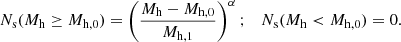
In this work, we adopted the HOD model described by Zheng et al. (2005), defined by five parameters (Mh, min, Mh, 1, σlog M, α, Mh, 0) that characterize the occupation of centrals and satellites within halos of a given mass Mh. In this model, the average occupation of central galaxies Nc is modeled by a smoothed step function:
![Mathematical equation: $$ \begin{aligned} N_{\rm c}(M_{\rm h}) = \frac{1}{2} \left[ 1 + \mathrm{erf} \left( \frac{\log M_{\rm h} - \log M_{\rm h, min}}{\sigma _{\log M}} \right) \right], \, \end{aligned} $$](/articles/aa/full_html/2025/10/aa53828-25/aa53828-25-eq13.gif) (10)
(10)
where σlog M represents the scatter in the SHMR and Mh, min is the characteristic halo mass for which 50% of halos host at least one central galaxy. The average satellite occupation Ns follows a power-law of slope α > 0, with the characteristic halo mass, Mh, 1, needed to host a satellite, for halos of mass greater than the Mh, 0 satellite cutoff mass,
 (11)
(11)
The total number of galaxies, Ntot, in a halo of mass, Mh, is then given by
![Mathematical equation: $$ \begin{aligned} N_{\rm tot}(M_{\rm h}) = N_{\rm c}(M_{\rm h}) \times \left[ \, 1 + N_{\rm s}(M_{\rm h}) \, \right] . \end{aligned} $$](/articles/aa/full_html/2025/10/aa53828-25/aa53828-25-eq15.gif) (12)
(12)
Some galaxy properties can be directly derived from the HOD model, such as the mean number density of galaxies, ng, the fraction of centrals, fcen, and satellites, fsat, or the mean galaxy bias, bg, expressed as below:
 (13)
(13)
 (14)
(14)
 (15)
(15)
 (16)
(16)
We used the package halomod (Murray et al. 2021)4 for computing the HOD model. Key elements of this model include the halo mass function dn(Mh, z)/dMh from Behroozi et al. (2013), the large-scale halo bias bh(Mh, z) from Tinker et al. (2010), a halo concentration-mass relationship from Duffy et al. (2008), a halo exclusion model based on double ellipsoids (Tinker et al. 2005), and a Navarro et al. (1997) halo profile. The galaxy spatial two-point correlation function, composed of a “one-halo” and a “two-halo term” (for correlations within a same halo and betweendistinct halos, respectively), is derived from these occupation distributions (see Asgari et al. 2023 for a detailed derivation). The ACF is finally computed using the Limber (1954) approximation, based on this spatial correlation function and the observed redshift distribution N(z) of each galaxysample.
While HOD models simplify the galaxy–halo connection by focusing solely on mass, it is acknowledged that other factors, such as halo formation history, can also influence the galaxy population within halos (e.g., Hearin et al. 2016). More complex HOD models, such as the one by Leauthaud et al. (2011), exist; however, since we aim to apply these models to high-z clustering with a low number of data points, we chose one with fewer free parameters. We note that the HOD model proposed by Zehavi et al. (2005) includes only three parameters, but it does not account for the scatter σlog M in the occupation of centrals. Numerous studies have demonstrated that this scatter exists and can affect clustering signals (e.g., Wechsler & Tinker 2018). We confirmed our choice of HOD model by redoing our analysis with Zehavi et al. (2005) model, which showed no substantial enhancement of our derived model constraints.
3.2.2. Nonlinearities in the halo bias
One key component of the halo model is the halo bias, bh, which quantifies how much halos are biased compared to the underlying dark matter distribution. The most widely used model of bh is the linear bias from Tinker et al. (2010), calibrated at large, linear scales in N-body simulations. While effective at large scales, this linear bias shows significant discrepancies in the transition region between the one- and two-halo terms. Studies such as Mead et al. (2015) and Jose et al. (2013) show that it under-predicts galaxy clustering in these “quasi-linear” regions (at scales of r ∼ 10 − 100 kpc), with discrepancies reaching up to 30%.
This deviation is attributed to the breakdown of linear perturbation theory at these scales, since halos form through the nonlinear collapse of overdensities in the dark matter fluctuation field, requiring a nonlinear approach. This is coupled to scale-dependent variations in bh, that primarily emerge from the shape of the halo profile (e.g., Tinker et al. 2005). Indeed, on large scales, these variations are negligible, allowing the halo center power spectrum to be simply expressed in terms of the linear matter power spectrum. However, at scales comparable to the size of individual halos, the halo profile becomes nonuniform, resulting in deviations from linear theory. This effect is expected to increase with redshift and halo mass, as the formation of rarer and then more highly biased halos in overdensities amplifies these nonlinearities.
However, incorporating nonlinearities into the halo model formalism for galaxy studies is challenging, and only a few models of nonlinear halo bias exist to date (e.g., Reed et al. 2009; Jose et al. 2016; Mead & Verde 2021). A nonlinear, scale-dependent (hereafter NL-SD) bias is typically constructed by measuring the ratio of the halo spatial correlation function to the matter one (written as ![Mathematical equation: $ b_{\mathrm{h}} = [\xi_{\mathrm{hh}}^{\mathrm{sim}}/\xi_{\mathrm{mm}}]^{1/2} $](/articles/aa/full_html/2025/10/aa53828-25/aa53828-25-eq20.gif) ) in N-body simulations across different redshifts and halo mass ranges, and comparing this to the large-scale ratio. A model for such a bias is provided by Jose et al. (2016, hereafter J16), expressed as:
) in N-body simulations across different redshifts and halo mass ranges, and comparing this to the large-scale ratio. A model for such a bias is provided by Jose et al. (2016, hereafter J16), expressed as:
 (17)
(17)
where bLS is the large-scale halo bias from Tinker et al. (2010) and ζ(r, Mh, z) is a NL-SD correction. Calibrating with the MXXL simulation (Angulo et al. 2012) for the range 0 ≤ z < 3 and MS-W7 (Guo et al. 2013; Pike et al. 2014) for 3 ≤ z < 5, J16 derived a fitting function for ζ and showed that the halo bias is strongly scale-dependent and nonlinear at scales of r ∼ 0.5 − 10 h−1 Mpc (further details on ζ are provided in Appendix D). This effect becomes stronger at higher redshifts and with increasing halo mass as halos become rarer. Such a bias will modify the halo correlation function ξhh – which is involved in the prediction of the galaxy ACF – that is now expressed as
![Mathematical equation: $$ \begin{aligned} 1 + \xi _{\rm hh}(r, M_{\rm h}^{\prime }, M_{\rm h}^{\prime \prime }, z) = \;&\bigr [ 1 + b_{\rm h}(r, M_{\rm h}^{\prime }, z) \, b_{\rm h}(r, M_{\rm h}^{\prime \prime }, z) \\&\xi _{\rm mm}(r, z) \bigr ] \times \Theta \left[ r - r_{\rm min}(M_{\rm h}^{\prime }, M_{\rm h}^{\prime \prime }) \right] \nonumber , \end{aligned} $$](/articles/aa/full_html/2025/10/aa53828-25/aa53828-25-eq22.gif) (18)
(18)
considering a pair of halos with masses Mh′ and Mh″. Here, Θ(r) is the Heaviside function that accounts for halo exclusion, suppressing the correlation at r < rmin in which rmin = min[R200(Mh′), R200(Mh″)] and R200(Mh) is the halo virial radius (from van den Bosch et al. 2013). This model of halo exclusion, used by J16 in its calibrations, is adapted to the halo finder used in our mass function calculations and prevents the exponential increase in the NL-SD halo bias at small scales.
Incorporating this correction into the halo model boosts the two-halo term of the galaxy correlation function at intermediate scales for z ≥ 2 − 3, as demonstrated by Jose et al. (2017), Harikane et al. (2018), Mead & Verde (2021), while leaving the one-halo term unchanged since halo bias does not affect the internal galaxy distribution within a halo. Observational clustering studies at z ∼ 3 (Jose et al. 2013; Barone-Nugent et al. 2014; Durkalec et al. 2015; Dalmasso et al. 2024a) have found that the one-to-two halo transition break becomes less pronounced, with clustering measurements following a power-law across all scales rather than a two-component model. We suggest that this effect arises because nonlinear processes cause early, massive halos to be more clustered and biased relative to dark matter, thereby boosting the two-halo term of galaxy clustering at intermediate scales, as modeled here by the J16 NL-SD model.
In this work, we first performed HOD modeling without the J16 bias across the full redshift range of z = 0.1 − 14. After implementing the correction in halomod, we repeated the analysis now incorporating the NL-SD bias, but starting from the bin 2.5 ≤ z < 3.5. This is because the J16 bias at z < 3 has been calibrated using the MXXL simulation, which shows significant discrepancies with our halo mass function, so we anticipated that it might overestimate the correction in this range. Nevertheless, our primary goal was not to achieve precise modeling of the correlation function with this correction, but to emphasize the importance of accounting for nonlinear effects on the halo bias at these scales and high redshifts. Indeed, there are several potential limitations to our implementation of their model. First, J16 z ≥ 3 fitting functions were calibrated using the MS-W7 simulation, which assumes a slightly different cosmology and halo mass function than the one adopted here. This discrepancy affects the rarity of halos of a given mass, a key parameter in the computation of the correction term. Additionally, while the J16 model was originally calibrated for 3 ≤ z ≤ 5, we extrapolated it to z > 5, though this approach inherently reduces its accuracy.
3.2.3. MCMC fitting
We ran a Markov chain Monte Carlo (MCMC) algorithm to fit HOD model parameters to our angular clustering measurements, using the emcee package (Foreman-Mackey et al. 2013). This method minimizes the χ2 value of clustering and number density measurements, within each redshift and stellar mass-limited bins (above a certain stellar mass threshold M⋆,th):
![Mathematical equation: $$ \begin{aligned} \chi ^2 =&\sum _{i,j}^{N_\theta } [w_{\rm obs}(\theta _i) - w_{\rm mod}(\theta _i)] \, C^{-1}_{ij} \, [w_{\rm obs}(\theta _j) - w_{\rm mod}(\theta _j)] \\&+ \left( \frac{n_{\rm g}^\mathrm{obs}(> M_{\star , \mathrm {th}}) - n_{\rm g}^\mathrm{mod}(> M_{\star , \mathrm {th}})}{\sigma _{n}} \right)^2 \nonumber , \end{aligned} $$](/articles/aa/full_html/2025/10/aa53828-25/aa53828-25-eq23.gif) (19)
(19)
where the model ACF has been corrected for the integral constraint as mentioned in Sect. 3.1. We excluded the largest angular scales (θ > 10−1 deg) from the fits at all redshifts as they are limited by the survey area. The smallest scales (θ < 2 × 10⁻⁴ deg) were also excluded at z ≤ 4 despite being above the survey resolution limit and size of the PSF, as they are likely affected by deblending issues which can bias the measurements (this is evidenced by the drop in the clustering signal at small scales not predicted by models in Fig. 6). At higher z, however, we kept this small-scale point in the fits, given the low number and high uncertainties of data points.
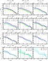 |
Fig. 6. Angular autocorrelation function of galaxies in the COSMOS-Web survey, in redshift and mass limited bins. Solid lines show the HOD best-fit models, with their 1σ uncertainties in shaded regions. For the two highest redshift bins, both conservative and extended samples are represented, with HOD best-fit models in dashed and solid lines, respectively. |
We chose to fit only the first three HOD parameters Mh, min, Mh, 1, and α in our model. Variations of the parameter σlog M have a weak impact on the correlation function relative to our error bars and are thus more difficult to constrain with our data. It is also slightly degenerate with Mh, min, as a higher scatter implies a lower Mh, min and vice versa. Therefore, we prioritized accurately constraining Mh, min. Values for σlog M range from 0.15 to 0.5 dex in both observations and simulations, with a different evolution with redshift and halo mass (see Porras-Valverde et al. 2024 for a compilation), but discrepancies can arise from the fact that it can contain both stellar mass measurement errors and intrinsic scatter in SHMR. We adopted a value of σlog M = 0.20 dex, which balances various results (e.g., Zheng et al. 2005; Conroy et al. 2006; Harikane et al. 2016; Cowley et al. 2019; Shuntov et al. 2022). Following other studies (Hatfield et al. 2018), we fixed Mh, 0 using the following equation,
 (20)
(20)
which has been derived in simulations up to z ≤ 3 by Conroy et al. (2006) and found in Contreras & Zehavi (2023) trends. We extrapolated it for z > 3, knowing that according to our tests, varying this parameter has a negligible effect on clustering results relative to our error bars in these regimes. The HOD parameters were re-fitted for each redshift bin as we opted not to model their intrinsic redshift evolution.
Furthermore, our initial MCMC runs revealed an issue where the algorithm got stuck on solutions exhibiting a flat one-halo term. We consider this solution highly unlikely to be physically relevant, as such a small-scale behavior is not observed in our measurements or in the literature. To solve this problem, we implemented a strict condition to reject any model whose one-halo term falls below the two-halo term at scales of θ < 10−4.
The MCMC used 30 walkers for a maximum of 6000 steps, stopping earlier if convergence criteria were met: 30 × τ < Niter and Δτ < 15% with τ the chain’s autocorrelation time and Niter the number of iterations. The chain started with random initial positions based on flat priors, chosen from typical values fitted on other studies in the literature (e.g., Zheng et al. 2007; Harikane et al. 2016; Shuntov et al. 2022): log(Mh, min/M⊙)∈[7, 15], log(Mh, 1/M⊙)∈[log(Mh, min/M⊙),16] and α ∈ [0.1, 2].
We also investigated the impact of our covariance matrices on the fit. If the covariance matrix shows excessively high or low correlations in the data relative to the mean, it might misguide the fit. To reduce these effects, we optimized the number of patches used in the jackknife computation. However, for some bins with unreliable covariance matrices (for the bins at z ≥ 8), we used only diagonal elements in the χ2 minimization.
Best fit parameters were derived using a Gaussian Kernel Density Estimation (KDE) across the three joint posterior distributions. The KDE was implemented using scipy.stats.gaussian_kde, which automatically adjusts the bandwidth for each dimension based on the data’s covariance matrix. Their lower and upper asymmetric uncertainties were computed in the 68% confidence interval. Model-derived quantities and their uncertainties were computed from the 16th, 50th, and 84th percentiles of the MCMC sample distribution. Parameters for all redshift and mass bins are listed in Appendix B.
4. Results
4.1. Angular clustering in COSMOS-Web
4.1.1. Clustering of mass-selected galaxies
We present in Fig. 6 the angular autocorrelation function of COSMOS-Web galaxies from z = 0.1 to 14 in redshift and mass-limited samples5, along with their best-fit HOD models (which will be discussed in Sect. 4.1.3).
Across all redshifts, we observe the familiar trend of increasing clustering with higher galaxy stellar mass thresholds. This trend aligns with the expectation that massive galaxies typically trace denser and more clustered regions of the Universe (e.g., Peebles 1980; Kaiser 1984).
The clustering deviates from a simple power-law at scales around θ ∼ 10−2 deg (equivalent to ∼0.3 Mpc in comoving coordinates at z ∼ 1, for example). This break signifies the transition between the clustering of galaxies within the same halo (the one-halo term) at small scales and the inter-halo clustering (two-halo term) at larger scales. This behavior is more pronounced for massive galaxies, as their massive halos host more satellites, enhancing the one-halo term. We note that clustering measurements drop at the lowest scales, most likely due to source deblending limitations in the survey, and at the highest scales (around θ ≥ 2 × 10⁻² deg for the COSMOS-Web field) because of the limited size of the survey.
The unusual high clustering signal at large scales in the redshift bin 0.6 ≤ z < 1.0 likely reflects the presence of the prominent filamentary structure known as the COSMOS Wall at z = 0.73 (Iovino et al. 2016). In the 5 ≤ z < 6 bin, we observe that the clustering is also abnormally high across all mass thresholds, potentially due to a field overdensity or SED fitting issues excluding sources near z ∼ 5 (see the source overdensity just before z = 5 in Fig. 2). Above z = 6, statistical uncertainties increase, complicating precise correlation function measurements. Notably, in the highest redshift bins, clustering follows a power law as the one-halo term becomes harder to probe. This agrees with other high-z studies (e.g., Magliocchetti et al. 2023, for 3 ≤ z < 5 passive galaxies). For instance, Jose et al. (2017) propose that at z ≥ 3, nonlinear scale-dependent halo bias amplifies the power at intermediate scales (∼0.5 − 1 Mpc), as discussed in Sect. 4.1.3. At z ≥ 8, clustering amplitudes for fixed mass thresholds are higher than at lower redshifts (+0.1 to 0.5 dex at r < 100 kpc), consistent with expectations: observed high-z galaxies are rarer and represent the most massive and luminous systems, likely hosted by the most massive halos forming early in the Universe (e.g., Chiang et al. 2017).
4.1.2. Comparison with the literature
While most of the surveys show very similar behaviors for clustering at low z, the high-z regime has not been extensively explored yet, and some discrepancies are still visible between different data. In Fig. 7, we show a non-exhaustive comparison with literature measurements at z ≥ 3, however with different sample selections: some are UV magnitude (MUV) limited, others are Lyman-break selected galaxies (LBGs).
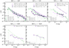 |
Fig. 7. Comparison of COSMOS-Web’s ACF with literature measurements (Barone-Nugent et al. 2014; Harikane et al. 2018; Cowley et al. 2018; Shuntov et al. 2022; Dalmasso et al. 2024a). Some works used UV magnitude-limited samples or LBG samples, so direct comparison with mass-limited samples is not possible. However, we chose to represent them since they are the only existing clustering measurements at z ≥ 8. |
For intermediate redshifts (3 ≤ z ≤ 6), our measurements align with those of Shuntov et al. (2022) in the COSMOS field, Cowley et al. (2018) in the SMUVS survey within COSMOS (Ashby et al. 2018), and Harikane et al. (2018) for LBGs observed in the HSC Subaru Strategic Program over 100 deg2 (Aihara et al. 2018a). In the 6 ≤ z < 8 range, while the shape of our clustering measurements matches those of Harikane et al. (2018), their amplitudes are more than 1 dex higher. This discrepancy is most likely due to incompleteness or potential errors in stellar mass or redshift estimates in the HSC survey, which – despite pushing the limits of ground-based high-z observations – probably detected only the brightest and most massive galaxies at z ∼ 6, leading to this higher measured clustering amplitude. Finally, in the highest redshift bin, we compare our results with those of Dalmasso et al. (2024a) for UV-bright galaxies at z ∼ 10.6 in the JADES survey (Eisenstein et al. 2023). Both the clustering amplitude and slope are similar. Given that JADES is deeper than COSMOS-Web and includes more JWST filters for sources at z > 10, this strengthens our confidence in our high-z sample. However, because their sample is limited by UV magnitude, directly comparing their measurements with ours is not straightforward. Nonetheless, since their UV limit (MUV < −15.5) is broad, it is more likely to correspond to a low mass threshold (e.g., 108 M⊙), with the resulting signal being primarily dominated by low-mass galaxies.
4.1.3. HOD models
The best-fit HOD models, along with their 1σ uncertainties, are represented by solid curves in Fig. 6, for the case where we did not correct for nonlinear halo bias. Detailed best-fit parameters and uncertainties are provided in Appendix B.
At low redshifts (z < 3), the HOD model closely matches the observational data across the range 4 × 10⁻⁴ < θ < 6 × 10⁻² deg. However, the largest angular scales are not well-fitted due to the model’s drop-off caused by the IC. Observed clustering at small scales is often higher than predicted, with a relative error Δw = (wobs − wmod)/wmod ≥ 150% for scales θ < 10−3 deg. This may occur if the satellite distribution profile within halos is different from our assumption in the HOD, resulting in a more tightly one-halo clustering. For z ≥ 3, discrepancies with the HOD model become more pronounced, especially at intermediate scales. Similar behavior has been reported in previous studies (e.g., Jose et al. 2013; Harikane et al. 2018) and may indicate the need to incorporate additional physical processes, such as nonlinearities in the halo bias assumed in the HOD model (see Sect. 3.2.2). In the bin 5 ≤ z < 6, the shape of the modeled clustering does not align with the observations, which is likely due to issues with the measurements and galaxy sample at this specific redshift bin since it is solved at z > 6. Finally, in some high-redshift bins such as z ≥ 10.5, the clustering amplitude is not as well constrained. This is most likely because there is also a constraint on number densities in the fit, which have smaller errors than clustering measurements since they are first-order statistics, less affected by field variations or sample size. As a result, number densities can have a stronger influence on the fit than clustering.
We explored HOD models incorporating the J16 NL-SD halo bias for galaxy clustering at z ≥ 2.5, as described in Sect. 3.2.2: best-fit models are presented in Appendix D. For an illustration, Fig. 8 shows the results for the 6 ≤ z < 8 bin, with and without the NL-SD halo bias. Adding this correction significantly reduces the relative error from Δw ≃ 1 − 2 to nearly 0 across scales 10−3 < θ < 2 × 10⁻² deg. This improvement is consistent across all redshift bins at z ≥ 2.5. We compared the χ2 values between the linear and NL-SD models, finding that χNL − SD2 < χlinear2 in 60% of cases across the full θ range, with a mean Δχ2 = χlinear2 − χNL − SD2 = +4. Nonetheless, some discrepancies arise for the most massive bins in certain redshift ranges (e.g., for samples with log(M⋆/M⊙)≥10.5 at 2.5 ≤ z < 3 or log(M⋆/M⊙)≥9.5 at 5 ≤ z < 6), where the nonlinear correction overpowers the one-halo term at intermediate scales, causing clustering to flatten at small scales. This behavior likely reflects limitations in the model calibration for very massive galaxies, where the nonlinear correction is overestimated and the one-halo term remains low. A more robust implementation of the NL-SD bias within our model, considering, for example, the same assumptions in cosmology and the halo model when deriving the nonlinear correction factor, will be required for accurate predictions of our high-redshift galaxy correlation functions.
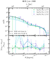 |
Fig. 8. ACF of galaxies in the bin 6 ≤ z < 8, and HOD best-fit models with and without a nonlinear scale-dependent halo bias (shown in dash-dotted and solid lines, respectively). Relative errors are presented in the bottom panel. |
While both models yield similar halo mass estimates and HOD-derived quantities (e.g., Fig. 9 shows a maximum difference of ∼0.25 dex in Mh, min), we continue our analysis with the HOD best-fit model without NL-SD bias for simplicity and interpretability. Nevertheless, including a NL-SD term in the halo bias and HOD formalism is likely essential to capture the power-law-like behavior of clustering observed at high redshift and to improve the modeling of halo and galaxy clustering.
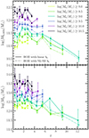 |
Fig. 9. Redshift evolution of the characteristic halo masses fitted in the HOD model for stellar mass-limited galaxy samples. Mh, min is the characteristic halo mass to host a central galaxy, Mh, 1 to host a satellite. Error bars are the 1σ uncertainties from the MCMC sample distribution, and quantities are shown for HOD models with and without nonlinear scale-dependent halo bias, respectively in dash-dotted and solid lines. |
4.2. Characteristic halo masses
Characteristic halo masses of galaxy samples are estimated via the HOD parameters fitted to the observations. Figure 9illustrates the evolution with redshift of the two Zheng et al. (2005) HOD characteristic halo masses, Mh, min to host a central galaxy and Mh, 1 to host a satellite, with their error bars computed as the 16th and 84th percentiles of the MCMC sample distribution. Consistent with previous findings, there is a general trend indicating that more massive galaxies are hosted by more massive halos across all redshifts. Notably, Mh, 1 typically exceeds Mh, min by approximately 1 dex, a relationship also observed in prior studies (e.g., Hatfield et al. 2019). However, a new observation emerges: at fixed stellar mass, Mh, min exhibits an increase with redshift, reaching a peak around redshift z ∼ 2 − 3, before subsequently decreasing. For a more comprehensive analysis of this phenomenon, we refer to Sect. 4.3.
Characteristic halo masses at z ≥ 6 are (see Appendix B):  for galaxies at 8.0 ≤ z < 10.5 with M⋆ ≥ 109 M⊙;
  for galaxies at 10.5 ≤ z < 14 with M⋆ ≥ 108.85 M⊙. We note that a similar halo mass estimate of Mh ≃ 1010.44 M⊙ for 10.5 ≤ z < 14 galaxies is found when using only number densities through abundance matching.
We can estimate the integrated star formation efficiency (SFE) εSF needed to convert baryons to stellar mass, assuming a baryonic fraction from the cosmological model ΛCDM fb ≈ 0.18785, as below:
 (21)
(21)
 (22)
(22)
where M⋆,th is the stellar mass threshold and M⋆,med the median stellar mass of the galaxy sample. This expression describes the growth of the stellar mass over the halo’s lifetime. The obtained results agree with ΛCDM model predictions; however, a high εSF ∼ 12 − 35% (according to εSF definitions; see the next section for more details) is needed to explain the range of stellar masses that we observe at z ≥ 8. This range is much higher than at lower z, where it does not reach values above ∼4% at similar halo mass.
4.3. Stellar-to-halo mass ratio
We can link the stellar masses of our galaxy samples with their corresponding characteristic halo masses − and consequently connecting galaxy to halo growth − by computing the SHMR. We present in Fig. 10 our inferred SHMR across the range z = 0.1 − 12, computed first as the ratio of the threshold stellar mass of each sample, M⋆,th, to their associated halo mass, Mh, min, as a function of halo mass6. The SHMR as the ratio of the galaxy sample’s median stellar mass, M⋆,med, over halo mass is also shown, as it gives different amplitudes and slightly different slopes. Both definitions are used in the literature (e.g., Harikane et al. 2016; Zaidi et al. 2024). While they both use the same halo mass, the first one gives a sense of the minimum star formation efficiency in producing central galaxies just above the threshold mass in halos of mass Mh, min; thus, it is then more influenced by the lower end of the stellar mass distribution in each sample. In contrast, the second definition connects the halo mass Mh, min to more massive central galaxies than the minimum mass required to be hosted by it, so it captures an average star formation efficiency in halos at this mass scale. Consequently, the latter SHMR tends to show a higher amplitude, as it reflects the contribution of more massive galaxies that dominate the median.
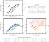 |
Fig. 10. Stellar-to-halo mass relationship in COSMOS-Web determined by HOD fitting of our clustering measurements. The integrated star formation efficiency is also shown from εSF = M⋆/(Mhfb). The point at 10.5 ≤ z < 14 is represented in dotted lines because it is considered less certain. Top: SHMR defined as the ratio M⋆,th/Mh,min. Bottom: SHMR defined M⋆,med/Mh,min (solid lines). It is split into two panels, z < 3 in the bottom left, and z ≥ 3 in the bottom right. The SHMR computed by abundance matching from Shuntov et al. (2025b) is also shown in dashed lines. |
We also display the SHMR derived from abundance matching in COSMOS-Web by Shuntov et al. (2025b), where the assumption that one halo hosts one galaxy is made. These two independent measurements of the SHMR show the same evolution with redshift, and their amplitudes are in agreement with each other in the case of the SHMR M⋆, med/Mh, min. The discrepancy in amplitude with the M⋆, th/Mh, min relation can be explained by the fact that, while abundance matching counts galaxies above a stellar mass threshold, it associates one galaxy to one halo, focusing on centrals without explicitly including satellites or scatter – in contrast with our HOD model. As a result, the typical halo mass hosting a central galaxy is lower in abundance matching. This is why the SHMR instead aligns with our measured one drawn using the median stellar mass, since it better captures the typical stellar mass of centrals and/or accounts for scatter.
The SFE εSF is also shown in Fig. 10 and we discuss its implications in Sect. 5. We also note that the SHMR presented in this work is a rough estimate for central galaxies because we are using Mh, min, which is the characteristic halo mass derived specifically for central galaxies. A more complex modeling of the SHMR (such as using Leauthaud et al. 2011 model) is beyond the scope of this work.
4.4. Satellite fractions
In addition to halo mass estimates, the HOD model derives central and satellite galaxy occupations, which can give further indications on the formation and merging of structures in the Universe. Figure 11 shows the evolution of the HOD-derived satellite fraction with redshift for fixed stellar mass thresholds, calculated using halomod based on Eq. (14). In the HOD model, satellites are defined as galaxies that orbit around a central galaxy, which resides at the center of the halo’s gravitational potential well. Globally, the fraction of satellite galaxies decreases with redshift, starting from 15 − 20% at z < 4 and decreasing to 1 − 5% at z > 4. As expected, the satellite fraction is higher for lower mass thresholds. The trends at z < 1 likely reflect a combination of limited survey volume at z < 0.5, which lowers the satellite fraction, and overdensities in the COSMOS field (such as the cluster at z = 0.7) which enhances it around z ∼ 1. Another drop is seen at 2.5 ≤ z < 3.0 for log(M⋆/M⊙)≥8.5 and ≥9.5 bins (also seen in the HOD modeling in COSMOS2020 by Shuntov et al. 2022), likely reflecting an overestimation of Mh, 1 in the HOD fit inherent to the COSMOS field, rather than a physical effect (see also Fig. 9). Then, the fraction decreases sharply between z = 1 and z = 2, after which the decline becomes more gradual, eventually reaching a plateau at some mass thresholds and approaching nearlyzero at z ≥ 8.
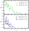 |
Fig. 11. Redshift evolution of the HOD-derived satellite fraction for mass-limited samples of galaxies. The point at 10.5 ≤ z < 14 is represented in dotted lines because it is considered less certain. |
This decrease is also seen in other clustering analyses (e.g., Hatfield et al. 2018; Harikane et al. 2018; Ishikawa et al. 2020), and more recently in Zaidi et al. (2024) in UDS + COSMOS fields up to z = 4.5. For the high-z regime, Bhowmick et al. (2018), for instance, also found fsat < 0.05 for galaxies with mass log(M⋆/M⊙)≥9.0 at z = 8 and z = 10, using HOD modeling in the BlueTides simulation (Feng et al. 2016). As cosmic time progresses, the Universe’s structure becomes more filamentary, small halos merge into larger and more massive ones, increasing the number of satellites per halo (see e.g., White & Frenk 1991; Bullock et al. 2001). The almost negligible fraction of satellite galaxies at z = 10 could reflect the early Universe’s initial stages, where fewer structures have formed and merged. However, our sample is likely biased toward the most massive and brightest galaxies, which are typically centrals, since satellites with M⋆ > 109 M⊙ at these redshifts are expected to be too rare to be detected by COSMOS-Web. Bhowmick et al. (2018) predicted a probability of less than 30% of observing satellites of mass log(M⋆/M⊙)≥9.0 around centrals of mass log(M⋆/M⊙) = 10.5 at z = 7.5 according to JWST limitations, a value that decreases with redshift. It is also important to note that our satellite fractions are lower (a difference of 0.01 to 0.05) than those reported in COSMOS2020 (Shuntov et al. 2022), independently of redshift, likely because they used the Leauthaud et al. (2011) HOD model that better constrains satellite and central galaxies at low redshifts.
4.5. Galaxy bias
Finally, we can derive the galaxy bias, bg, which is defined as the ratio between the clustering of galaxies wg and the clustering of dark matter (DM) particles, wDM,
 (23)
(23)
This effect depends on various physical processes, such as feedback, gas cooling, star formation, and black hole accretion, which influence the distribution and evolution of galaxies differently from that of dark matter. Estimations of this bias are derived using Eq. (16) in the halomod package, based on the fitted halo occupation distribution for each galaxy sample.
Current halo and galaxy formation models predict that halos initially form in rare fluctuations of the primordial matter density field, leading to high bias and clustering in the most massive halos, in which the first galaxies are expected to form (Kaiser 1984). This suggests that the galaxy bias should increase at earlier epochs. However, new studies of high-z galaxies challenge this simple view. Indeed, two main scenarios are proposed to explain the overabundance of UV-bright, massive galaxies observed at z ≥ 8 with JWST (Sect. 1). The first suggests higher scatter in the UV magnitude – halo mass relation (or stochasticity, e.g., Mason et al. 2023; Mirocha & Furlanetto 2023; Kravtsov & Belokurov 2024), allowing low-mass halos to host UV-bright galaxies due to starbursts that make them bright enough to be observed before their massive stars die (Sun et al. 2023). This scatter may be more pronounced in lower-mass halos, which dominate the early Universe, as the galaxies inhabiting them could be more sensitive to feedback or environmental effects, triggering cycles of starbursts (Gelli et al. 2024). Although one might argue that our sample is mass-selected and therefore less affected by such stochastic effects, at high redshift, the SED-fitting estimation of the mass relies only on the rest-frame UV and optical. For example, at z > 10, the reddest band probed by our set of filters is the rest-frame u. This could lead to overestimating the stellar mass of starbursting galaxies, hence artificially increasing the SHMR stochasticity as well. The second scenario suggests a tighter galaxy–halo connection with high star formation efficiency in massive halos (e.g., Dekel et al. 2023; Yung et al. 2024). A study by Muñoz et al. (2023) showed that both scenarios are degenerate in the UVLF but anticipated that galaxy bias measurements from JWST would help distinguish between them. A bias with little variation across stellar mass thresholds would support high stochasticity, since the apparent massive end would be, in fact, dominated by lower-mass, less biased halos. In contrast, a high bias with strong mass variation would favor a high star formation efficiency, suggesting that massive galaxies reside in massive halos.
In Fig. 12, we represent the evolution of our galaxy bias measurements with redshift for different stellar mass thresholds, along with model predictions for samples limited by UV magnitude from Muñoz et al. (2023) and Gelli et al. (2024). The first one has been calibrated on UVLF measurements from HST (Bouwens et al. 2021) and early JWST observations (Pérez-González et al. 2023; Finkelstein et al. 2023; Harikane et al. 2023), while Gelli et al. (2024) calibrated its halo mass-dependent scatter based on the zoom-in simulation FIRE-2 following Sun et al. (2023). To compare these models to our mass-limited results, we computed simplified versions of the SMF and the UVLF. By matching the cumulative number of galaxies in our sample below a certain MUV threshold, we determined the corresponding M⋆ threshold. We verified that using the median of the MUV − M⋆ distribution gives consistent results, with differences of less than 5%. This procedure led to matching estimates presented in Table 1.
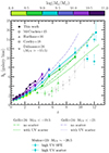 |
Fig. 12. Evolution of the galaxy bias with redshift, for different stellar mass thresholds, derived from the HOD modeling of our clustering measurements. The point at z ∼ 12 is represented in dotted lines because it is considered less certain. Predictions of the galaxy bias as a function of UV magnitude by Muñoz et al. (2023) and Gelli et al. (2024) are superposed, with and without implementation of a large scatter in the MUV − Mh relationship to explain the overabundance of bright galaxies at high-z. Literature measurements from McCracken et al. (2015), Harikane et al. (2016), and Cowley et al. (2018) are shown in colors corresponding to their sample threshold mass. The exception is Dalmasso et al. (2024b), which is in gray, since it corresponds to a stellar mass that is below our bin minimum. |
Stellar mass lower thresholds in units of log(M⋆/M⊙) corresponding to MUV upper thresholds, derived by matching cumulative numbers of galaxies in our sample as a function of both properties.
When comparing to the predictions, our bias measurements appear to support the second explanation: the hypothesis that high star formation efficiency in massive halos drives the observed abundance of galaxies at high redshifts. Specifically, our results for log(M⋆/M⊙)≥8.5 and 4 ≤ z < 10 align more closely with the Gelli et al. (2024) model without UV scatter for MUV < −19.5. The z ≃ 12 point was placed in the log(M⋆/M⊙)≥9.0 panel for visualization purposes, although it corresponds to galaxies with log(M⋆/M⊙)≥8.85, making it compatible with the no-scatter model for MUV < −19.5 galaxies. Similarly, for log(M⋆/M⊙)≥9.5 and 4 ≤ z < 6, the model without scatter for MUV < −21 is within 1.5σ of our measurements. Furthermore, the Muñoz et al. (2023) prediction without scatter falls within the 1σ uncertainties at z ∼ 12, while the one with scatter is ∼2σ lower.
However, strict conclusions require a mass-limited model of stochasticity at high redshift, ideally calibrated with COSMOS-Web data. In our analysis, we consider UV-bright galaxies detected at high-z to be comparable to our massive galaxies. While these galaxies are likely star-forming and UV-emitting, selection effects may introduce biases, and a direct comparison with models based on MUV − Mh scatter is not straightforward. For instance, UV-limited samples could miss massive galaxies with low star formation rates, whereas mass-limited samples might overlook low-mass galaxies that experience short-lived starbursts. Additionally, we did not fit the scatter σlog M in the HOD, which may lead to bias if an intrinsic scatter is present. Nonetheless, we also estimated the galaxy bias using Eq. (23) by comparing the dark matter clustering predictions from N-body simulations at z ∼ 12 to our galaxy clustering measurements, which suggests an even higher bg than what we derive from the HOD model. This indicates that our conclusions remain robust despite these potential biases.
5. Discussion
5.1. What we can learn about the galaxy-halo connection at z ≥ 6 from clustering
Recent observations, including the present study, highlight the presence of highly efficient star formation and massive galaxies at z ≥ 6. Our results, supported by clustering and HOD modeling, show that these high-z galaxies are residing in more massive halos than those expected by pre-JWST galaxy formation models or simulations (see the discussion in Sect. 5.2.2). This is consistent with results from other JWST surveys. For instance, in the COSMOS-Web field, Casey et al. (2024) reported luminous and massive sources at z > 10 believed to be undergoing rapid starbursts, and Shuntov et al. (2025b) reveals an overabundance of massive galaxies at high redshift from stellar mass function measurements in the same field.
To this day, several explanations have been proposed to account for these observations, which can be broadly divided into five categories: (I) an intrinsic high star formation efficiency at early times for example because of effective cold gas accretion and fragmentation (e.g., Fujimoto et al. 2024; Faisst et al. 2025), feedback-free star formation (hereafter FFB; Dekel et al. 2023; Li et al. 2024) or high merger-induced star formation (Duan et al. 2025; II) a stochastic and bursty star formation at high-z (e.g., Mason et al. 2023; III) an overestimation of inferred stellar masses for example because of a top-heavy IMF at high-z (see e.g., Trinca et al. 2024; Lu et al. 2025; IV) a different treatment of dust attenuation, eliminating the need for evolving SFE (Ferrara et al. 2023; V) or a change in cosmology, as early dark energy (Klypin et al. 2021; Liu et al. 2024). Each of these scenarios translates into a different galaxy–halo connection, and some of them can lead to distinct clustering patterns due to differences in how galaxies populate halos of various masses, while other observables, such as the UVLF, are degenerate (Muñoz et al. 2023).
Focusing on the FFB model, we find that our derived SFE and halo masses are compatible with its predictions. This model posits that at early times, star-forming clouds in halos with masses between 1010.8 × [(1 + z)/10]−6.2 ≤ Mh < 1012 M⊙ could achieve star formation efficiencies of up to 50 to 100%, given a brief window of ∼1 Myr where feedback mechanisms are ineffective. Our estimated halo masses for galaxies with M⋆ > 108.5 − 9 M⊙ at z ≥ 8 fall within this predicted regime. Our derived SFE values at z ≥ 8 agree with the FFB predictions assuming a FFB maximum efficiency around ϵFFB, max ≃ 0.2, and are lying about 2σ above no-FFB expectations (calculated using the ffb_predict code7, from Li et al. 2024). These efficiencies naturally decrease with cosmic time as radiative feedback becomes more prominent and the star-forming clouds become less dense, aligning with the decline we see in the SHMR. Additionally, this model reproduces the COSMOS-Web SMF well when ϵFFB, max increases with both redshift and stellar mass (see Shuntov et al. 2025b for the detailed analysis). Further investigations on this and other high-z models are left for future work. We also note that stochasticity in the MUV − Mh relation, which may be connected to this bursty star formation regime, could influence the evolution of galaxy bias, which we explored in Sect. 4.5.
Moreover, halo properties play a crucial role in regulating star formation. For instance, the halo accretion rate is one of the factors that controls the availability of gas for star formation (White & Frenk 1991), while inflows and outflows are influenced by the depth of the halo’s potential well, all of which can be related to halo mass. The high merger rates at early times (Duan et al. 2025) further enhance star formation efficiency. Therefore, linking galaxies to their host halo mass is essential. Currently, this is often done using abundance matching, a method that relies on strong assumptions and is typically applied to incomplete samples, potentially introducing biases, and does not account for scatter in the MUV − Mh or M⋆ − Mh relations.
Thus, the information from galaxy clustering is currently the most robust way to connect galaxies at z ≥ 6 to halos and estimate their host properties. Galaxies should not be viewed as isolated systems; rather, their star formation is influenced by the large-scale structures in which they live. Additionally, we emphasise that any viable scenario for the early Universe must simultaneously account for the high SFE observed at z ≥ 6 and its gradual decline over time until approximately z ∼ 3, as captured in the SHMR (see Sect. 5.2.1).
5.2. The interplay between stellar and dark matter growth across time
5.2.1. Evolution of the SHMR with redshift
The SHMR shows the interplay between the dark matter accretion rate and the conversion from gas to stars inside galaxies. Here, we propose a simple scenario to explain the evolution of the SHMR observed in Fig. 10 from the early Universe at z > 10 to the present.
At high redshift, the SHMR is greater than at lower redshifts for a given halo mass, indicating a higher star formation efficiency in the early Universe. As discussed in Sect. 5.1, this high efficiency for z > 8 can be attributed to star formation occurring in bursty episodes with star-formation timescale shorter than supernova explosion timescale, leading to negligible (or none at all) impact of feedback from stellar or radiative processes (FFB model; Dekel et al. 2023). Renzini (2025) also suggests that the lack of angular momentum in the very early Universe could lead locally (at the globular cluster scale) to very high baryon concentrations and consequently to elevated SFE (see also Loeb 2024). In these very dense regions, gravitational acceleration could also be high enough to overcome momentum injection from stellar feedback, allowing efficient star formation (e.g., Boylan-Kolchin 2025).
Over time, halos keep accreting matter. The high accretion rate in the early Universe leads to strong turbulence, which could prevent star formation due to the turbulent-pressure support (e.g., Andalman et al. 2025). This can be combined with outflows, which drive part of the accreted gas out of the halos, making the SHMR progressively decreasing. As galaxies grow, feedback mechanisms such as stellar feedback or AGN activity become more efficient. In massive halos, AGNs will accumulate mass through accretion and expel or heat surrounding gas more forcefully (e.g., Man & Belli 2018). In lower-mass halos, massive stars will die and generate strong stellar winds. Hence, star formation will become less and less efficient at a given stellar mass threshold, as shown in Fig. 9. As the ability to form stars from halo gas accretion diminishes, gas accumulates in halos faster than it can be converted into stars, further reducing the SHMR as time progresses.
However, at z ∼ 2 − 3, this trend reverses, in particular for low-mass galaxies. The observed SHMR begins to increase, indicating that the efficiency of central stellar mass growth becomes higher relative to dark matter growth. This corresponds to the redshift at which the halo growth rate slows and often reaches a plateau, after which halo mass varies more gradually (see mass accretion rates from Behroozi et al. 2013 for example, or Lilly et al. 2013). Meanwhile, delayed star formation can still occur due to the gas reservoir accumulated within halos, leading to an increase in the SHMR. This behavior is also in agreement with a type of “downsizing” scenario, where the peak of star formation shifts to lower-mass halos (Mh < 1012 M⊙) as cosmic time progresses (see e.g., Cowie et al. 1996; Neistein et al. 2006; Conroy & Wechsler 2009). Although we cannot directly probe the evolution of the SHMR peak and its high-mass end with COSMOS-Web, we observe that its amplitude at fixed halo mass increases with time (for Mh < 1012 M⊙), indicating that in low-mass halos star formation becomes more efficient at later times. According to this scenario, these low-mass halos would then host younger galaxies than their more massive counterparts, in opposition to the hierarchical scenario of structure formation (De Lucia et al. 2006).
Using the semi-empirical model UNIVERSEMACHINE8 (Behroozi et al. 2019) – the only simulated catalog reproducing the same trend as our observations (see Sect. 5.2.2) – we show in Fig. 13 the ratio of the star formation rate (SFR) of galaxies to the halo mass accretion rate (Ṁh) over time. In halo mass bins, halo mass accretion rates have been computed analytically with the formula of Behroozi et al. (2013), and we take the median SFR of UNIVERSEMACHINE galaxies hosted by these halos. Starting from high-redshifts, we observe a decreasing ratio, indicating that dark matter halos are growing faster than stellar mass. Around a mean redshift of z ≃ 3.8 (with this transition redshift increasing for more massive halos), this trend reverses, showing an increase in the ratio as dark matter growth becomes less efficient than star formation. This trend holds up to a halo mass of log(Mh/M⊙)≃12.5, beyond which the ratio only decreases from high to low redshift, but we do not explore this high-mass regime since it falls outside the scope of our observational data. This pattern further supports our proposed scenario, demonstrating the evolving relationship between galaxy and halo growth rates over time. We also compared this to measurements in COSMOS-Web, plotting the median SFR of galaxies at the threshold mass as a function of redshift and halo mass Mh, min. The results are consistent with those in UNIVERSEMACHINE in both amplitude and trend. However, due to the large scatter in median SFR and the fact that we do not have the results as a continuous function of Mh, min and z, we focus here on presenting the simulation results only for a clearer understanding of thescenario.
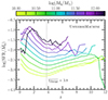 |
Fig. 13. Evolution of the ratio between star formation rate and halo mass accretion rate as a function of redshift, in the semi-empirical model UNIVERSEMACHINE. In halo mass bins of width 0.25 dex, the ratio is computed as the halo accretion rate from the analytical formula in Behroozi et al. (2013) formula over the median SFR of galaxies hosted by halos in the mass bin. A transition in the ratio behavior is observed at a mean redshift |

Shuntov et al. (2025b) presents evolutionary tracks for halos (and their associated stellar mass) formed at z = 10, z = 6, and z = 2 with the same initial halo mass, constructed using the Dekel et al. (2013) halo mass growth function combined with an SFE derived from their SHMR. For instance, they show that a halo formed at z = 6 or z = 10 experiences an increase in SFE, which peaks and then declines once the halo reaches a mass of ∼1012.5 M⊙. As a result, such halos that formed before z ≃ 3.5 would have built up most of their stellar mass by that time. Further investigations are needed to quantitatively describe this scenario, including, for example, analysis of halo and galaxy kinematics or gas properties that could explain this trend in the SHMR. However, this is beyond the scope of thecurrent work.
5.2.2. Comparison of our SHMR with observations, simulations, and models
There is currently a significant discrepancy in the observations, models, and simulations regarding the evolution of SHMR with redshift. If we focus on the Universe at z > 4, some studies show no evolution (Sun & Furlanetto 2016; Stefanon et al. 2017, 2021), while others see the SHMR decreasing with increasing redshift (Tacchella et al. 2018; Zhu et al. 2020) or the opposite (Finkelstein et al. 2015; Harikane et al. 2016; Moster et al. 2018; Behroozi et al. 2019).
5.2.2.1. Comparison with other observations.
Our findings are consistent with those in the COSMOS field, such as Shuntov et al. (2022), who report a similar trend in the SHMR for halos with Mh < 1012 M⊙ using the COSMOS2020 catalog. Leauthaud et al. (2011), using weak lensing measurements, also observed an increasing SHMR from z = 2 to z = 0 along with a shift toward lower masses for the pivot halo mass (the mass where star formation is most efficient). Recent results from Zaidi et al. (2024), based on clustering and HOD modeling in the UDS + COSMOS fields up to z = 4.5, show a change in slope in the SHMR between Mh ∼ 1010.5 and 1012.5 M⊙, with a 50% increase in SHMR at Mh = 1011.5 M⊙ from 3.5 ≤ z < 4.5 to 0.2 ≤ z < 0.5. These findings do not show significant discrepancies with ours, and differences in HOD models, SHMR definitions, and data completeness may explain minor variations.
At higher redshifts, to our knowledge, few studies probe the mass and redshift ranges we cover. Harikane et al. (2016, 2018) found a similar trend, with a decrease in SHMR from z = 7 to z = 4 using the clustering of LBGs in HSC data. Conversely, Stefanon et al. (2021) claims no redshift evolution in the SHMR from z = 6 to z = 10 using abundance matching. However, this study mixes different fields (HUDF, XDF, GOODS, and all five CANDELS fields) and relies on Spitzer/IRAC data, which has known limitations for galaxies at z > 8 due to factors like shallower depth (the program they use is ∼1.5 magnitude shallower than COSMOS-Web’s F444W depth) and challenges with deblending because of lower resolution. Their sample is likely incomplete, with only 800 LBGs, and their stellar mass function does not match ours in COSMOS-Web (as shown in Shuntov et al. 2025b), being higher at 5.5 ≤ z < 7.5 and lower at 7.5 ≤ z < 10, which suggests a lower SHMR at high redshifts than what we find.
5.2.2.2. Comparison with models.
Secondly, we compare our results to semi-empirical models, starting with UNIVERSEMACHINE which is shown in the bottom-right panel of Fig. 14. This model exhibits a similar redshift trend to our observations, with a decreasing SHMR from z = 11 to z = 2 − 3 and a turnover at z = 2 − 3. UNIVERSEMACHINE has been calibrated using observational constraints before JWST, such as the stellar mass function and clustering measurements up to z ∼ 10. This indicates that information about this evolution was likely already present in the observational results before JWST. Secondly, the EMERGE empirical model (Moster et al. 2018) also shows a decreasing SHMR from z = 0.1 to z = 4 and an increase of 30% from z = 4 to z = 8. As in the case of UNIVERSEMACHINE, it is constrained by observed SFRs, SMFs, and cosmic star formation rate densities up to z ∼ 10. EMERGE computes the SFR of individual galaxies as the product of an instantaneous star formation efficiency and their host halo’s growth rate, linking stellar history to halo formation. This approach introduces scatter in the SHMR, resulting in higher stellar masses in low-mass halos at high redshift, similar to the effects of bursty star formation histories at z > 4. Another empirical model, from Tacchella et al. (2018), follows a similar approach to EMERGE but forces a redshift-independent star formation efficiency, ϵSF(Mh), and is calibrated solely on the UVLF at z = 4. Consequently, this model predicts a steadily decreasing SHMR from z = 4 to 14, which contrasts with both EMERGE, UNIVERSEMACHINE, and our observational trends.
 |
Fig. 14. Comparison of the observational SHMR in COSMOS-Web with results from various hydrodynamical simulations and the semi-empirical model UNIVERSEMACHINE. Solid lines represent the observational SHMR M⋆,th/Mh,min, obtained from HOD fitting of mass-limited galaxy clustering measurements in COSMOS-Web. The point at 10.5 ≤ z < 14 is represented in dotted lines because it is considered less certain. The dashed and other lines represent the SHMR in the simulations computed similarly to the observations, where Mh, min is the halo mass at which 50% of halos host a central galaxy with a stellar mass above M⋆,th. Top left: SHMR from TNG100 simulation snapshots, computed at the mean redshifts of each observational redshift range. Top right: SHMR from Horizon-AGN light-cone, calculated over the same redshift ranges as the observations, but limited to z ≤ 6. Bottom right: Same from UNIVERSEMACHINE light-cone in the COSMOS field, matching the observational redshift ranges. Bottom left: Same for high-z simulations (THESAN-1, FirstLight, OBELISK), computed from snapshots at mean redshifts from z ∼ 5 to z ∼ 12. |
5.2.2.3. Comparison with simulations.
Finally, we compare our results with several state-of-the-art hydrodynamical simulations, some of them being specially built to study the high-z Universe: TNG100 (Pillepich et al. 2018; Nelson et al. 2018; Marinacci et al. 2018; Naiman et al. 2018; Springel et al. 2018), HORIZON-AGN (Dubois et al. 2014), THESAN-1 (Kannan et al. 2022), FirstLight (Ceverino et al. 2017), OBELISK (Trebitsch et al. 2021). A summary of their main characteristics (resolutions, mass definitions, etc.) can be found in Appendix E.
We did the exercise to measure the SHMR from the simulations the same way as our observational SHMR: in central galaxy samples limited in mass by M⋆,th, we computed the characteristic halo mass Mh, min as the halo mass at which 50% of halos host a central galaxy of mass above M⋆,th. We verified that this recovers the true SHMR computed using individual galaxies and their host halo masses, confirming that the SHMR as M⋆,th/Mh,min is a good proxy for the true SHMR in observations as well: the median difference between the two was less than 7%, while for M⋆,med/Mh,min it is of the order of 15 − 20%. The comparison between our observational SHMR and simulation results is presented in Fig. 14. Most simulations conducted before JWST do not reproduce the observed abundance of massive galaxies, nor do they predict the high star formation efficiency seen at z > 6. So rather than focusing solely on the amplitude of the stellar-to-halo mass ratios, we emphasize their redshift evolution to determine whether they display a similar behavior to the observed SHMR, showing this characteristic turnover around z = 2 − 3. For a more detailed comparison of the SHMR in COSMOS with TNG100 and HORIZON-AGN up to z = 5 (in terms of amplitudes and slopes), we refer toShuntov et al. (2022).
The TNG100 simulation is in good agreement with observed SHMR amplitudes and slopes for z < 1. However, it does not show a distinct evolution with redshift, except for a gradual change in slope for low-mass halos. This slope becomes shallower at higher redshifts, indicating a higher star formation efficiency at a fixed halo mass as redshift increases, but only for halos with masses below 1010.5 M⊙. The change in slope is not clearly observed in the data, and the SFE at high redshift is not as high as measured in the observations. For halos above this mass range, the SHMR consistently decreases with increasing redshift.
Similarly, HORIZON-AGN simulation shows little evolution in SHMR from z = 0.1 to z = 3, and there is no indication of a turnover in its evolution. It is then followed by a sharp decline for 3 < z < 6, but this may be explained by the underestimation of the mass function at z > 4 in the simulation due to resolution limits (see Appendix E). We note that the SHMR amplitude is generally not comparable to observations, as previously noted in studies such as Hatfield et al. (2019) or Shuntov et al. (2022), likely due to the overestimation of galaxy masses in low-mass halos.
Simulations specifically designed to study the high-redshift Universe show discrepancies among themselves, and with the data. As JWST has revealed more massive objects than anticipated, these simulations generally contain lower halo and galaxy mass ranges than observed, with amplitudes that are also not directly comparable. Additionally, almost none of them replicate the same redshift evolution observed in our data. For instance, the OBELISK simulation, which is centered on an overdense region within a small volume, only shows a decrease in the SHMR of ∼0.5 dex from z = 9 to z = 3. While the THESAN-1 simulations show a more comparable amplitude, the SHMR appears constant with redshift, as expected since THESAN extends the TNG model with radiative transfer and thus naturally looks like TNG’s low-z SHMR. Among these simulations, only the FirstLight simulation hints at an increasing SHMR for z > 4, but it is a zoom-in simulation of ∼300 galaxies and could be biased by cosmic variance effects or incompleteness in the computation of the SHMR.
These figures highlight the significant discrepancies between current simulations and observations, as well as inconsistencies among the simulations themselves, particularly those specialised for the epoch of reionization. This may be the result of wrong calibrations in the simulations at high-z with pre-JWST data, but might also depend on changes in the physical processes involved in star formation (e.g., the FFB model). It is noteworthy that even simulations based on the same model, like TNG100 and THESAN, yield significantly different SHMR amplitudes, likely due to their calibration on low versus high-redshift observations. This suggests that the trend of higher star formation efficiency at early times might have already been hinted at in pre-JWST literature. Our results offer valuable constraints on star formation efficiency and the galaxy–halo connection from z = 0.1 up to the highest redshifts, which can guide the development of more accurate future simulations and help refine how galaxies populate halos at z > 10.
5.3. Limitations of this work
5.3.1. High-redshift sample and completeness
This study relied solely on photometric data for deriving photometric redshifts and estimating stellar masses through SED fitting. At high redshifts, where only a few IR bands are available in COSMOS-Web, identifying the Lyman break and constraining galaxy SEDs pose challenges (see, e.g., Narayanan et al. 2024, for stellar mass recovering at z > 7). Hence, potential contamination from lower or higher redshift objects could bias our clustering analyses. To mitigate this effect, rigorous cleaning procedures were applied to our high-redshift sample (see Sect. 2.2.2). To assess residual contamination after this cleaning, we computed cross-correlations between our selected redshift bins (Appendix C). Ideally, a contamination-free sample in a given redshift bin would yield a null signal when cross-correlated to another redshift bin. As mentioned in Sect. 2.2.2, for low-z bins, the signal remains minimal, except in adjacent bins due to photo-z uncertainties sometimes spanning a large redshift range. For redshift bins at z ≥ 8.0, the correlation signal is more pronounced, particularly with redshift bins at 2.5 ≤ z ≤ 5, yet still at least 3× lower than the autocorrelation signal. This suggests that despite inherent photo-z uncertainties, our selection across large redshift bins remains robust.
Another argument supporting our sample selection is that we consistently observe a non-null signal in the autocorrelation function at z > 10, even with different SED assumptions. If our sample were solely contaminated by low-z galaxies, we would not expect to detect any significant clustering. To test this, we computed the autocorrelation by randomly selecting galaxies within the redshift range 0 < z < 5, and found a constant clustering signal around w(θ)∼0, which contrasts with the behavior observed in the z > 10 sample, further indicating the presence of high-redshift galaxies in our sample. Nonetheless, systematic effects may persist in the photometric redshift estimates, influenced, for example, by choices in dust attenuation models used in the SED fitting code, particularly affecting galaxies at z > 6.
Concerns regarding the completeness of our samples arise when considering galaxies at high redshifts and low stellar masses. By implementing a magnitude threshold based on comparisons with the deeper JWST survey PRIMER, we ensured that at least 80% of galaxies below this limit were detected. However, our selection is probably biased toward brighter and more compact galaxies at these high redshifts. Although the fraction of satellite galaxies is expected to be low at z ≥ 8 and for the masses we observe, faint low-mass satellites could still be missed by our detection, potentially leading to an underestimation of clustering at small scales. Having more satellites would lead to lower estimates of halo masses required to host central galaxies and potentially higher SHMR. Conversely, for z < 8, we are confident in the completeness of our survey, suggesting that the observed trends in the SHMR evolution with redshift (particularly at z > 3) are unlikely to be significantly altered by completeness issues.
We also examined the impact of objects with AGNs dominating their rest-frame UV or optical emission, along so-called LRDs (Matthee et al. 2024) at high redshifts, on our clustering measurements. These objects were identified as described in Sect. 2.2.2, and we compared the z ≥ 4 autocorrelation functions with and without them. We found no significant change in the amplitude or slope of our clustering measurements. Although AGNs can be major contaminants in the SMF due to their SEDs being degenerate with those of high-mass or highly dust-obscured galaxies (see, Shuntov et al. 2025b or e.g., Schaerer & de Barros 2009; Barro et al. 2024), their presence does not appear to affect the clustering. This insinuates that the clustering of our sample is not only driven by AGN-dominated objects at high-z. However, a robust AGN selection and analysis of their clustering properties across all redshifts are outside the scope of this work.
5.3.2. Stellar mass estimates
The construction of our samples, and therefore the inferred HOD parameters based on their associated clustering, depend on the accuracy of galaxy stellar mass estimates. Determining stellar masses heavily relies on the choice of the initial mass function (IMF), which remains uncertain at high redshifts. In this study, we adopted the Chabrier (2003) IMF; however, a top-heavy IMF would lead to lower stellar mass estimates and number densities (see, e.g., Cameron et al. 2024). While this modification would not change the clustering signal, it would result in a lower SHMR and a reduced star formation efficiency. According to predictions from the ASTREUS simulation (Cueto et al. 2024), their evolving IMF (top-heavy at high-z) leads to a decrease in stellar masses of approximately 0.6 dex at z = 8 and 0.7 dex at z = 12 for the halo mass range derived in this study. Even accounting for this adjustment, our SHMR M⋆,th/Mh at z ≥ 8 remains ∼0.5 dex higher than the z = 1 ratio at a same halo mass. Moreover, Shuntov et al. (2025b) shows that the ASTRAEUS simulation indicates excessively high number densities at low masses compared to the observational stellar mass function in COSMOS-Web. Further investigation is needed to determine the shape of the primordial IMF, such as studying the metallicity of high-redshift galaxies through a spectroscopic survey, since a higher number of massive stars would contribute more to the metal enrichment of these galaxies (e.g.,Pallottini et al. 2025).
Estimating the stellar mass of galaxies at z ≥ 8 can also be biased as a result of the limited number of filters for detecting their SED and Balmer breaks. Studies have shown that including MIRI data leads to lower stellar mass estimates compared to NIRCam-only, as the Balmer break for z ≥ 12 galaxies falls beyond the F444W filter, and MIRI can probe nebular emission lines, helping to rule out older star populations and better constrain dust models (e.g., Song et al. 2023; Papovich et al. 2023). In our sample, around 30% of galaxies at z ≥ 5 have MIRI data, but otherwise Papovich et al. (2023) finds that mass over-estimations are typically < 0.25 dex at z < 6 and 0.37 dex at 6 ≤ z < 9. Dust attenuation models can also introduce mass deviations, up to 0.35 dex at z = 7 − 8 according to Markov et al. (2023). Despite these uncertainties, stellar masses at z ≥ 8, after correction for these factors, give an SHMR that remains ∼1 dex higher than the ones at z < 3. Lastly, we note that the transition from the Planck Collaboration VI (2020) cosmological model used in this work to a standard ΛCDM model (with H0 = 70 kms−1Mpc−1, Ωm, 0 = 0.3, ΩΛ, 0 = 0.7) – which is used in LePHARE – only reduces masses by −0.030 dex at z = 0 and −0.0175 dex at z = 10.
6. Conclusion
This work explores the angular autocorrelation function of mass-limited samples of galaxies within the COSMOS-Web survey, a field of 0.54 deg2 observed with JWST. It spans a range of photometric redshifts from z = 0.1 to z ∼ 12, making it the first measurement of clustering at z > 10 with a mass-limited sample. This highlights the unique capabilities of COSMOS-Web in examining large-scale structures and the environments of high-redshift galaxies, as it is less affected by cosmic variance compared to other current JWST fields with smaller areas. The aim of this research was to examine the galaxy-halo connection consistently across 13.4 Gyr of cosmic history, using HOD modeling. Clustering remains the most robust method for estimating halo masses at these high redshifts, which is crucial for establishing the link between galaxies and their host halos and for understanding their role in regulating star formation. The main conclusions of this work are as follows.
-
Clustering measurements from z = 0.1 to z ∼ 12 follow the well-established trend, where more massive galaxies exhibit higher clustering amplitudes. The clustering signal at z ≥ 8 is strong, as expected given the observed massive galaxies are likely to be hosted in massive, early-forming halos; this result is also consistent with other literature results.
-
Clustering at z ≥ 2.5 is best fitted with a HOD model incorporating a nonlinear scale-dependent halo bias, which boosts the correlation signal at quasi-linear scales (r∼ 10–100 kpc). This adjustment accounts for the rarity of halos capable of hosting the massive and bright galaxies we observed, which are highly biased toward nonlinear fluctuations of the dark matter field.
-
From HOD fitting on clustering, we estimated the halo masses to be
 for galaxies at 8.0 ≤ z < 10.5 with log(M⋆/M⊙)≥9;
  for galaxies at 10.5 ≤ z < 14 with log(M⋆/M⊙)≥8.85. This suggests a higher integrated star formation efficiency at high redshift compared to lower redshift, with values exceeding εSF > 12 − 36% according to the adopted definition. Such high efficiencies can be explained, for instance, by the feedback-free burst model (Dekel et al. 2023), which is consistent with the halo mass regime of ourestimates.
 -
The evolution of the galaxy bias with redshift and with stellar mass thresholds favors the scenario of high star formation efficiency in massive halos (instead of high MUV − Mh scatter) as the primary driver of the abundance of high-z galaxies observed with JWST, although further modeling of stochasticity as a function of stellar mass is needed for conclusive results.
-
The SHMR evolves significantly with redshift in the range 10.5 ≤ log(Mh, min/M⊙)≤12.5, decreasing by ∼1 dex from z ∼ 10 to z ∼ 3. This decline reflects reduced star formation efficiency over time, potentially driven by more efficient feedback processes (e.g., AGN growth or stellar and/or radiative feedback), whereas halos accrete matter exponentially. At z ≃ 2 − 3, dark matter growth reaches a plateau while star formation might continue thanks to the gas stored in halos, causing the SHMR to rise again.
-
Observations, models, and simulations reveal significant discrepancies in the evolution of the SHMR with redshift. Some observations suggest a decline in the SHMR at z > 4 and some indicate no evolution or an increase. Hydrodynamical simulations often fail to capture the high SHMR or its redshift trends, emphasizing the need for improved calibrations or treatment of physical processes across cosmic time. Semi-empirical models such as EMERGE and UNIVERSEMACHINE, calibrated on observations up to z = 10, are able to successfully reproduce trends that are similar to ours by linking star formation efficiencies to halo mass, halo accretion rate, and redshift.
Building on this study, a future project will aim to separate the COSMOS-Web sample into star-forming and quiescent galaxies across various redshift and mass ranges. By performing autocorrelation and cross-correlation measurements up to z = 5, we will explore how the environment influences star formation and quenching processes. Understanding these mechanisms could provide insights into the evolution of the high-redshift galaxies discussed in this work, which may be the progenitors of the quiescent galaxies seen at z ∼ 3 − 5.
A future spectroscopic survey, such as the COSMOS-3D (JWST Cycle 3 Program GO #5893), will enhance mass and redshift estimates for high-z galaxies in COSMOS-Web. Spectroscopic data will reduce low-z contamination and uncertainties in our clustering and SHMR measurements, leading to more reliable galaxy properties and connection to their host dark matter halos.
Data availability
Our measurements of clustering and SHMR can be found in tabulated form at https://github.com/LouisePaquereau/GalClustering_COSMOS-Web_Paquereau2025.
Depths are measured in “empty” apertures of 0.15″ radius for NIRCam and 0.5″ for MIRI, which contain no objects in order to provide a realistic estimation of the background noise (Shuntov et al. 2025a).
We provide our clustering measurements at https://github.com/LouisePaquereau/GalClustering_COSMOS-Web_Paquereau2025
We provide our SHMR measurements at https://github.com/LouisePaquereau/GalClustering_COSMOS-Web_Paquereau2025
Acknowledgments
We thank the anonymous referee for their careful reading and helpful feedback. LP acknowledges the thesis funding from the Centre National d’Etudes Spatiales (CNES) and the Ecole Doctorale Astronomie et Astrophysique d’Ile-de-France. The authors acknowledge the funding of the French Agence Nationale de la Recherche for the project iMAGE (grant ANR-22-CE31-0007). This work was made possible by utilizing the CANDIDE cluster at the Institut d’Astrophysique de Paris. The cluster was funded through grants from the PNCG, CNES, DIM-ACAV, the Euclid Consortium, and the Danish National Research Foundation Cosmic Dawn Center (DNRF140). It is maintained by Stephane Rouberol. The authors acknowledge the contributions of the COSMOS collaboration. The French contingent of the COSMOS team is partly supported by the Centre National d’Etudes Spatiales (CNES). Support for this work was provided by NASA through grant JWST-GO-01727 awarded by the Space Telescope Science Institute, which is operated by the Association of Universities for Research in Astronomy, Inc., under NASA contract NAS 5-26555. This work is based in part on observations made with the NASA/ESA/CSA James Webb Space Telescope. The data were obtained from the Mikulski Archive for Space Telescopes at the Space Telescope Science Institute, which is operated by the Association of Universities for Research in Astronomy, Inc., under NASA contract NAS 5-03127 for JWST. The HST-COSMOS program was supported through NASA grant HSTGO-09822. More information on the COSMOS survey is available at https://cosmos.astro.caltech.edu. Based in part on observations collected at the European Southern Observatory under ESO programs 179.A-2005, 198.A-2003, 104.A-0643, 110.25A2 and 284.A-5026 and on data obtained from the ESO Science Archive Facility with DOI https://doi.org/10.18727/archive/52, and on data products produced by CANDIDE and the Cambridge Astronomy Survey Unit on behalf of the UltraVISTA consortium.
References
- Aihara, H., Arimoto, N., Armstrong, R., et al. 2018a, PASJ, 70, S4 [NASA ADS] [Google Scholar]
- Aihara, H., Armstrong, R., Bickerton, S., et al. 2018b, PASJ, 70, S8 [NASA ADS] [Google Scholar]
- Aihara, H., AlSayyad, Y., Ando, M., et al. 2022, PASJ, 74, 247 [NASA ADS] [CrossRef] [Google Scholar]
- Akins, H. B., Casey, C. M., Lambrides, E., et al. 2025, ApJ, 991, 37 [Google Scholar]
- Andalman, Z. L., Teyssier, R., & Dekel, A. 2025, MNRAS, 540, 3350 [Google Scholar]
- Angulo, R. E., Springel, V., White, S. D. M., et al. 2012, MNRAS, 426, 2046 [NASA ADS] [CrossRef] [Google Scholar]
- Arnouts, S., Moscardini, L., Vanzella, E., et al. 2002, MNRAS, 329, 355 [Google Scholar]
- Arnouts, S., Le Floc’h, E., Chevallard, J., et al. 2013, A&A, 558, A67 [NASA ADS] [CrossRef] [EDP Sciences] [Google Scholar]
- Asgari, M., Mead, A. J., & Heymans, C. 2023, Open J. Astrophys., 6, 39 [NASA ADS] [CrossRef] [Google Scholar]
- Ashby, M. L. N., Caputi, K. I., Cowley, W., et al. 2018, ApJS, 237, 39 [CrossRef] [Google Scholar]
- Barbary, K. 2016, J. Open Source Software, 1, 58 [NASA ADS] [CrossRef] [Google Scholar]
- Barone-Nugent, R. L., Trenti, M., Wyithe, J. S. B., et al. 2014, ApJ, 793, 17 [Google Scholar]
- Barro, G., Pérez-González, P. G., Kocevski, D. D., et al. 2024, ApJ, 963, 128 [CrossRef] [Google Scholar]
- Behroozi, P. S., Wechsler, R. H., & Conroy, C. 2013, ApJ, 770, 57 [NASA ADS] [CrossRef] [Google Scholar]
- Behroozi, P., Wechsler, R. H., Hearin, A. P., & Conroy, C. 2019, MNRAS, 488, 3143 [NASA ADS] [CrossRef] [Google Scholar]
- Bertin, E., & Arnouts, S. 1996, A&AS, 117, 393 [NASA ADS] [CrossRef] [EDP Sciences] [Google Scholar]
- Bertin, E., Schefer, M., Apostolakos, N., et al. 2020, in Astronomical Data Analysis Software and Systems XXIX, eds. R. Pizzo, E. R. Deul, J. D. Mol, J. de Plaa, & H. Verkouter, ASP Conf. Ser., 527, 461 [NASA ADS] [Google Scholar]
- Bhowmick, A. K., Campbell, D., Di Matteo, T., & Feng, Y. 2018, MNRAS, 480, 3177 [CrossRef] [Google Scholar]
- Bouwens, R. J., Oesch, P. A., Stefanon, M., et al. 2021, AJ, 162, 47 [NASA ADS] [CrossRef] [Google Scholar]
- Bower, R. G., Benson, A. J., Malbon, R., et al. 2006, MNRAS, 370, 645 [Google Scholar]
- Boylan-Kolchin, M. 2025, MNRAS, 538, 3210 [Google Scholar]
- Bruzual, G., & Charlot, S. 2003, MNRAS, 344, 1000 [NASA ADS] [CrossRef] [Google Scholar]
- Bryan, G. L., & Norman, M. L. 1998, ApJ, 495, 80 [NASA ADS] [CrossRef] [Google Scholar]
- Bullock, J. S., Kravtsov, A. V., & Weinberg, D. H. 2001, ApJ, 548, 33 [NASA ADS] [CrossRef] [Google Scholar]
- Calzetti, D., Armus, L., Bohlin, R. C., et al. 2000, ApJ, 533, 682 [NASA ADS] [CrossRef] [Google Scholar]
- Cameron, A. J., Katz, H., Witten, C., et al. 2024, MNRAS, 534, 523 [NASA ADS] [CrossRef] [Google Scholar]
- Carnall, A. C., Cullen, F., McLure, R. J., et al. 2024, MNRAS, 534, 325 [NASA ADS] [CrossRef] [Google Scholar]
- Carniani, S., Hainline, K., D’Eugenio, F., et al. 2024, Nature, 633, 318 [CrossRef] [Google Scholar]
- Casey, C. M., Kartaltepe, J. S., Drakos, N. E., et al. 2023, ApJ, 954, 31 [NASA ADS] [CrossRef] [Google Scholar]
- Casey, C. M., Akins, H. B., Shuntov, M., et al. 2024, ApJ, 965, 98 [NASA ADS] [CrossRef] [Google Scholar]
- Ceverino, D., Glover, S. C. O., & Klessen, R. S. 2017, MNRAS, 470, 2791 [NASA ADS] [CrossRef] [Google Scholar]
- Chabrier, G. 2003, PASP, 115, 763 [Google Scholar]
- Chemerynska, I., Atek, H., Furtak, L. J., et al. 2024, MNRAS, 531, 2615 [NASA ADS] [CrossRef] [Google Scholar]
- Chiang, Y.-K., Overzier, R. A., Gebhardt, K., & Henriques, B. 2017, ApJ, 844, L23 [Google Scholar]
- Chuang, C.-Y., Jespersen, C. K., Lin, Y.-T., Ho, S., & Genel, S. 2024, ApJ, 965, 101 [Google Scholar]
- Conroy, C., & Wechsler, R. H. 2009, ApJ, 696, 620 [NASA ADS] [CrossRef] [Google Scholar]
- Conroy, C., Wechsler, R. H., & Kravtsov, A. V. 2006, ApJ, 647, 201 [Google Scholar]
- Contreras, S., & Zehavi, I. 2023, MNRAS, 525, 4257 [Google Scholar]
- Cooray, A., & Sheth, R. 2002, Phys. Rep., 372, 1 [Google Scholar]
- Coupon, J., Arnouts, S., van Waerbeke, L., et al. 2015, MNRAS, 449, 1352 [NASA ADS] [CrossRef] [Google Scholar]
- Cowie, L. L., Songaila, A., Hu, E. M., & Cohen, J. G. 1996, AJ, 112, 839 [Google Scholar]
- Cowley, W. I., Caputi, K. I., Deshmukh, S., et al. 2018, ApJ, 853, 69 [NASA ADS] [CrossRef] [Google Scholar]
- Cowley, W. I., Caputi, K. I., Deshmukh, S., et al. 2019, ApJ, 874, 114 [NASA ADS] [CrossRef] [Google Scholar]
- Cueto, E. R., Hutter, A., Dayal, P., et al. 2024, A&A, 686, A138 [NASA ADS] [CrossRef] [EDP Sciences] [Google Scholar]
- Curtis-Lake, E., Carniani, S., Cameron, A., et al. 2023, Nat. Astron., 7, 622 [NASA ADS] [CrossRef] [Google Scholar]
- Dalmasso, N., Leethochawalit, N., Trenti, M., & Boyett, K. 2024a, MNRAS, 533, 2391 [Google Scholar]
- Dalmasso, N., Trenti, M., & Leethochawalit, N. 2024b, MNRAS, 528, 898 [Google Scholar]
- Davis, M., Efstathiou, G., Frenk, C. S., & White, S. D. M. 1985, ApJ, 292, 371 [Google Scholar]
- De Lucia, G., Springel, V., White, S. D. M., Croton, D., & Kauffmann, G. 2006, MNRAS, 366, 499 [NASA ADS] [CrossRef] [Google Scholar]
- Dekel, A., Zolotov, A., Tweed, D., et al. 2013, MNRAS, 435, 999 [Google Scholar]
- Dekel, A., Sarkar, K. C., Birnboim, Y., Mandelker, N., & Li, Z. 2023, MNRAS, 523, 3201 [NASA ADS] [CrossRef] [Google Scholar]
- Duan, Q., Conselice, C. J., Li, Q., et al. 2025, MNRAS, 540, 774 [Google Scholar]
- Dubois, Y., Pichon, C., Welker, C., et al. 2014, MNRAS, 444, 1453 [Google Scholar]
- Duffy, A. R., Schaye, J., Kay, S. T., & Dalla Vecchia, C. 2008, MNRAS, 390, L64 [Google Scholar]
- Durkalec, A., Le Fèvre, O., Pollo, A., et al. 2015, A&A, 583, A128 [NASA ADS] [CrossRef] [EDP Sciences] [Google Scholar]
- Eisenstein, D. J., Willott, C., Alberts, S., et al. 2023, ApJ, submitted, [arXiv:2306.02465] [Google Scholar]
- Euclid Collaboration (Ilbert, O., et al.) 2021, A&A, 647, A117 [NASA ADS] [CrossRef] [EDP Sciences] [Google Scholar]
- Faisst, A. L., Yang, L., Brinch, M., et al. 2025, ApJ, 980, 204 [Google Scholar]
- Feng, Y., Di-Matteo, T., Croft, R. A., et al. 2016, MNRAS, 455, 2778 [NASA ADS] [CrossRef] [Google Scholar]
- Ferrara, A., Pallottini, A., & Dayal, P. 2023, MNRAS, 522, 3986 [NASA ADS] [CrossRef] [Google Scholar]
- Finkelstein, S. L., Song, M., Behroozi, P., et al. 2015, ApJ, 814, 95 [Google Scholar]
- Finkelstein, S. L., Bagley, M. B., Arrabal Haro, P., et al. 2022, ApJ, 940, L55 [NASA ADS] [CrossRef] [Google Scholar]
- Finkelstein, S. L., Bagley, M. B., Ferguson, H. C., et al. 2023, ApJ, 946, L13 [NASA ADS] [CrossRef] [Google Scholar]
- Finkelstein, S. L., Leung, G. C. K., Bagley, M. B., et al. 2024, ApJ, 969, L2 [NASA ADS] [CrossRef] [Google Scholar]
- Foreman-Mackey, D., Hogg, D. W., Lang, D., & Goodman, J. 2013, PASP, 125, 306 [Google Scholar]
- Franco, M., Akins, H. B., Casey, C. M., et al. 2024, ApJ, 973, 23 [NASA ADS] [CrossRef] [Google Scholar]
- Franco, M., Casey, C. M., Akins, H. B., et al. 2025a, arXiv e-prints [arXiv:2508.04791] [Google Scholar]
- Franco, M., Casey, C. M., Koekemoer, A. M., et al. 2025b, ApJ, submitted, [arXiv:2506.03256] [Google Scholar]
- Fujimoto, S., Finkelstein, S. L., Burgarella, D., et al. 2023, ApJ, 955, 130 [NASA ADS] [CrossRef] [Google Scholar]
- Fujimoto, S., Ouchi, M., Kohno, K., et al. 2024, Nat. Astron., accepted, [arXiv:2402.18543] [Google Scholar]
- Gelli, V., Mason, C., & Hayward, C. C. 2024, ApJ, 975, 192 [NASA ADS] [CrossRef] [Google Scholar]
- Gouin, C., Gavazzi, R., Pichon, C., et al. 2019, A&A, 626, A72 [NASA ADS] [CrossRef] [EDP Sciences] [Google Scholar]
- Greene, J. E., Labbe, I., Goulding, A. D., et al. 2024, ApJ, 964, 39 [CrossRef] [Google Scholar]
- Groth, E. J., & Peebles, P. J. E. 1977, ApJ, 217, 385 [NASA ADS] [CrossRef] [Google Scholar]
- Guo, Q., White, S., Angulo, R. E., et al. 2013, MNRAS, 428, 1351 [NASA ADS] [CrossRef] [Google Scholar]
- Harikane, Y., Ouchi, M., Ono, Y., et al. 2016, ApJ, 821, 123 [NASA ADS] [CrossRef] [Google Scholar]
- Harikane, Y., Ouchi, M., Ono, Y., et al. 2018, PASJ, 70, S11 [NASA ADS] [CrossRef] [Google Scholar]
- Harikane, Y., Ouchi, M., Oguri, M., et al. 2023, ApJS, 265, 5 [NASA ADS] [CrossRef] [Google Scholar]
- Harish, S., Kartaltepe, J. S., Liu, D., et al. 2025, ApJ, accepted, [arXiv:2506.03306] [Google Scholar]
- Hatfield, P. W., & Jarvis, M. J. 2017, MNRAS, 472, 3570 [Google Scholar]
- Hatfield, P. W., Bowler, R. A. A., Jarvis, M. J., & Hale, C. L. 2018, MNRAS, 477, 3760 [NASA ADS] [CrossRef] [Google Scholar]
- Hatfield, P. W., Laigle, C., Jarvis, M. J., et al. 2019, MNRAS, 490, 5043 [NASA ADS] [CrossRef] [Google Scholar]
- Hearin, A. P., Zentner, A. R., van den Bosch, F. C., Campbell, D., & Tollerud, E. 2016, MNRAS, 460, 2552 [NASA ADS] [CrossRef] [Google Scholar]
- Hildebrandt, H., van Waerbeke, L., & Erben, T. 2009, A&A, 507, 683 [NASA ADS] [CrossRef] [EDP Sciences] [Google Scholar]
- Ilbert, O., Arnouts, S., McCracken, H. J., et al. 2006, A&A, 457, 841 [NASA ADS] [CrossRef] [EDP Sciences] [Google Scholar]
- Ilbert, O., Arnouts, S., Le Floc’h, E., et al. 2015, A&A, 579, A2 [NASA ADS] [CrossRef] [EDP Sciences] [Google Scholar]
- Iovino, A., Petropoulou, V., Scodeggio, M., et al. 2016, A&A, 592, A78 [NASA ADS] [CrossRef] [EDP Sciences] [Google Scholar]
- Ishikawa, S., Kashikawa, N., Tanaka, M., et al. 2020, ApJ, 904, 128 [NASA ADS] [CrossRef] [Google Scholar]
- Jarvis, M., Bernstein, G., & Jain, B. 2004, MNRAS, 352, 338 [Google Scholar]
- Jespersen, C. K., Cranmer, M., Melchior, P., et al. 2022, ApJ, 941, 7 [NASA ADS] [CrossRef] [Google Scholar]
- Jespersen, C. K., Steinhardt, C. L., Somerville, R. S., & Lovell, C. C. 2025, ApJ, 982, 23 [Google Scholar]
- Jose, C., Subramanian, K., Srianand, R., & Samui, S. 2013, MNRAS, 429, 2333 [Google Scholar]
- Jose, C., Lacey, C. G., & Baugh, C. M. 2016, MNRAS, 463, 270 [Google Scholar]
- Jose, C., Baugh, C. M., Lacey, C. G., & Subramanian, K. 2017, MNRAS, 469, 4428 [NASA ADS] [CrossRef] [Google Scholar]
- Kaiser, N. 1984, ApJ, 284, L9 [NASA ADS] [CrossRef] [Google Scholar]
- Kannan, R., Garaldi, E., Smith, A., et al. 2022, MNRAS, 511, 4005 [NASA ADS] [CrossRef] [Google Scholar]
- Katz, H., Rosdahl, J., Kimm, T., et al. 2023, Open J. Astrophys., 6, 44 [NASA ADS] [CrossRef] [Google Scholar]
- Kaviraj, S., Laigle, C., Kimm, T., et al. 2017, MNRAS, 467, 4739 [NASA ADS] [Google Scholar]
- Khostovan, A. A., Kartaltepe, J. S., Salvato, M., et al. 2025, arXiv e-prints [arXiv:2503.00120] [Google Scholar]
- Klypin, A., Poulin, V., Prada, F., et al. 2021, MNRAS, 504, 769 [NASA ADS] [CrossRef] [Google Scholar]
- Koekemoer, A. M., Aussel, H., Calzetti, D., et al. 2007, ApJS, 172, 196 [Google Scholar]
- Kokorev, V., Atek, H., Chisholm, J., et al. 2025, ApJ, 983, L22 [Google Scholar]
- Kravtsov, A., & Belokurov, V. 2024, arXiv e-prints [arXiv:2405.04578] [Google Scholar]
- Kroupa, P. 2001, MNRAS, 322, 231 [NASA ADS] [CrossRef] [Google Scholar]
- Kümmel, M., Bertin, E., Schefer, M., et al. 2020, in Astronomical Data Analysis Software and Systems XXIX, eds. R. Pizzo, E. R. Deul, J. D. Mol, J. de Plaa, & H. Verkouter, ASP Conf. Ser., 527, 29 [Google Scholar]
- Labbé, I., van Dokkum, P., Nelson, E., et al. 2023, Nature, 616, 266 [CrossRef] [Google Scholar]
- Lacey, C., & Cole, S. 1993, MNRAS, 262, 627 [NASA ADS] [CrossRef] [Google Scholar]
- Laigle, C., Davidzon, I., Ilbert, O., et al. 2019, MNRAS, 486, 5104 [Google Scholar]
- Landy, S. D., & Szalay, A. S. 1993, ApJ, 412, 64 [Google Scholar]
- Leauthaud, A., Tinker, J., Behroozi, P. S., Busha, M. T., & Wechsler, R. H. 2011, ApJ, 738, 45 [NASA ADS] [CrossRef] [Google Scholar]
- Lee, K.-S., Giavalisco, M., Gnedin, O. Y., et al. 2006, ApJ, 642, 63 [NASA ADS] [CrossRef] [Google Scholar]
- Li, Z., Dekel, A., Sarkar, K. C., et al. 2024, A&A, 690, A108 [NASA ADS] [CrossRef] [EDP Sciences] [Google Scholar]
- Lilly, S. J., Carollo, C. M., Pipino, A., Renzini, A., & Peng, Y. 2013, ApJ, 772, 119 [NASA ADS] [CrossRef] [Google Scholar]
- Limber, D. N. 1954, ApJ, 119, 655 [NASA ADS] [CrossRef] [Google Scholar]
- Liu, W., Zhan, H., Gong, Y., & Wang, X. 2024, MNRAS, 533, 860 [NASA ADS] [CrossRef] [Google Scholar]
- Loeb, A. 2024, Res. Notes Am. Astron. Soc., 8, 182 [Google Scholar]
- Lu, S., Frenk, C. S., Bose, S., et al. 2025, MNRAS, 536, 1018 [Google Scholar]
- Madau, P. 1995, ApJ, 441, 18 [NASA ADS] [CrossRef] [Google Scholar]
- Magliocchetti, M., Santini, P., Merlin, E., & Pentericci, L. 2023, MNRAS, 526, L8 [Google Scholar]
- Man, A., & Belli, S. 2018, Nat. Astron., 2, 695 [NASA ADS] [CrossRef] [Google Scholar]
- Marinacci, F., Vogelsberger, M., Pakmor, R., et al. 2018, MNRAS, 480, 5113 [NASA ADS] [Google Scholar]
- Markov, V., Gallerani, S., Pallottini, A., et al. 2023, A&A, 679, A12 [NASA ADS] [CrossRef] [EDP Sciences] [Google Scholar]
- Mason, C. A., Trenti, M., & Treu, T. 2023, MNRAS, 521, 497 [NASA ADS] [CrossRef] [Google Scholar]
- Matthee, J., Naidu, R. P., Brammer, G., et al. 2024, ApJ, 963, 129 [NASA ADS] [CrossRef] [Google Scholar]
- McCracken, H. J., Milvang-Jensen, B., Dunlop, J., et al. 2012, A&A, 544, A156 [NASA ADS] [CrossRef] [EDP Sciences] [Google Scholar]
- McCracken, H. J., Wolk, M., Colombi, S., et al. 2015, MNRAS, 449, 901 [NASA ADS] [CrossRef] [Google Scholar]
- Mead, A. J., & Verde, L. 2021, MNRAS, 503, 3095 [NASA ADS] [CrossRef] [Google Scholar]
- Mead, A. J., Peacock, J. A., Heymans, C., Joudaki, S., & Heavens, A. F. 2015, MNRAS, 454, 1958 [NASA ADS] [CrossRef] [Google Scholar]
- Milvang-Jensen, B., Freudling, W., Zabl, J., et al. 2013, A&A, 560, A94 [NASA ADS] [CrossRef] [EDP Sciences] [Google Scholar]
- Mirocha, J., & Furlanetto, S. R. 2023, MNRAS, 519, 843 [Google Scholar]
- Moster, B. P., Somerville, R. S., Newman, J. A., & Rix, H.-W. 2011, ApJ, 731, 113 [Google Scholar]
- Moster, B. P., Naab, T., & White, S. D. M. 2018, MNRAS, 477, 1822 [Google Scholar]
- Muñoz, J. B., Mirocha, J., Furlanetto, S., & Sabti, N. 2023, MNRAS, 526, L47 [CrossRef] [Google Scholar]
- Murray, S. G., Diemer, B., Chen, Z., et al. 2021, Astron. Comput., 36, 100487 [NASA ADS] [CrossRef] [Google Scholar]
- Naidu, R. P., Oesch, P. A., Setton, D. J., et al. 2022a, arXiv e-prints [arXiv:2208.02794] [Google Scholar]
- Naidu, R. P., Oesch, P. A., van Dokkum, P., et al. 2022b, ApJ, 940, L14 [NASA ADS] [CrossRef] [Google Scholar]
- Naiman, J. P., Pillepich, A., Springel, V., et al. 2018, MNRAS, 477, 1206 [Google Scholar]
- Narayanan, D., Lower, S., Torrey, P., et al. 2024, ApJ, 961, 73 [NASA ADS] [CrossRef] [Google Scholar]
- Navarro, J. F., Frenk, C. S., & White, S. D. M. 1997, ApJ, 490, 493 [Google Scholar]
- Navarro-Carrera, R., Rinaldi, P., Caputi, K. I., et al. 2024, ApJ, 961, 207 [CrossRef] [Google Scholar]
- Neistein, E., van den Bosch, F. C., & Dekel, A. 2006, MNRAS, 372, 933 [NASA ADS] [CrossRef] [Google Scholar]
- Nelson, D., Pillepich, A., Springel, V., et al. 2018, MNRAS, 475, 624 [Google Scholar]
- Oke, J. B., & Gunn, J. E. 1983, ApJ, 266, 713 [NASA ADS] [CrossRef] [Google Scholar]
- Ouchi, M., Shimasaku, K., Okamura, S., et al. 2004, ApJ, 611, 685 [NASA ADS] [CrossRef] [Google Scholar]
- Overzier, R. A., Bouwens, R. J., Illingworth, G. D., & Franx, M. 2006, ApJ, 648, L5 [NASA ADS] [CrossRef] [Google Scholar]
- Pallottini, A., Ferrara, A., Gallerani, S., et al. 2025, A&A, 699, A6 [NASA ADS] [CrossRef] [EDP Sciences] [Google Scholar]
- Papovich, C., Cole, J. W., Yang, G., et al. 2023, ApJ, 949, L18 [NASA ADS] [CrossRef] [Google Scholar]
- Peacock, J. A., & Smith, R. E. 2000, MNRAS, 318, 1144 [Google Scholar]
- Peebles, P. J. E. 1980, The Large-Scale Structure of the Universe (Princeton University Press) [Google Scholar]
- Pérez-González, P. G., Costantin, L., Langeroodi, D., et al. 2023, ApJ, 951, L1 [CrossRef] [Google Scholar]
- Pike, S. R., Kay, S. T., Newton, R. D. A., Thomas, P. A., & Jenkins, A. 2014, MNRAS, 445, 1774 [NASA ADS] [CrossRef] [Google Scholar]
- Pillepich, A., Nelson, D., Hernquist, L., et al. 2018, MNRAS, 475, 648 [Google Scholar]
- Planck Collaboration VI. 2020, A&A, 641, A6 [NASA ADS] [CrossRef] [EDP Sciences] [Google Scholar]
- Porras-Valverde, A. J., Forbes, J. C., Somerville, R. S., et al. 2024, ApJ, 976, 148 [Google Scholar]
- Pozzetti, L., Bolzonella, M., Zucca, E., et al. 2010, A&A, 523, A13 [NASA ADS] [CrossRef] [EDP Sciences] [Google Scholar]
- Reed, D. S., Bower, R., Frenk, C. S., Jenkins, A., & Theuns, T. 2009, MNRAS, 394, 624 [Google Scholar]
- Renzini, A. 2025, MNRAS, 536, L8 [Google Scholar]
- Roche, N., & Eales, S. A. 1999, MNRAS, 307, 703 [NASA ADS] [CrossRef] [Google Scholar]
- Rodriguez-Gomez, V., Sales, L. V., Genel, S., et al. 2017, MNRAS, 467, 3083 [Google Scholar]
- Salim, S., Boquien, M., & Lee, J. C. 2018, ApJ, 859, 11 [Google Scholar]
- Salpeter, E. E. 1955, ApJ, 121, 161 [Google Scholar]
- Sawicki, M., Arnouts, S., Huang, J., et al. 2019, MNRAS, 489, 5202 [NASA ADS] [Google Scholar]
- Schaerer, D., & de Barros, S. 2009, A&A, 502, 423 [NASA ADS] [CrossRef] [EDP Sciences] [Google Scholar]
- Sérsic, J. L. 1963, Boletin de la Asociacion Argentina de Astronomia La Plata Argentina, 6, 41 [Google Scholar]
- Shuntov, M., McCracken, H. J., Gavazzi, R., et al. 2022, A&A, 664, A61 [NASA ADS] [CrossRef] [EDP Sciences] [Google Scholar]
- Shuntov, M., Akins, H. B., Paquereau, L., et al. 2025a, A&A, submitted, [arXiv:2506.03243] [Google Scholar]
- Shuntov, M., Ilbert, O., Toft, S., et al. 2025b, A&A, 695, A20 [NASA ADS] [CrossRef] [EDP Sciences] [Google Scholar]
- Smith, R. E., Peacock, J. A., Jenkins, A., et al. 2003, MNRAS, 341, 1311 [Google Scholar]
- Song, J., Fang, G., Lin, Z., Gu, Y., & Kong, X. 2023, ApJ, 958, 82 [NASA ADS] [CrossRef] [Google Scholar]
- Springel, V., Pakmor, R., Pillepich, A., et al. 2018, MNRAS, 475, 676 [Google Scholar]
- Stefanon, M., Bouwens, R. J., Labbé, I., et al. 2017, ApJ, 843, 36 [NASA ADS] [CrossRef] [Google Scholar]
- Stefanon, M., Bouwens, R. J., Labbé, I., et al. 2021, ApJ, 922, 29 [NASA ADS] [CrossRef] [Google Scholar]
- Steinhardt, C. L., Jespersen, C. K., & Linzer, N. B. 2021, ApJ, 923, 8 [NASA ADS] [CrossRef] [Google Scholar]
- Sun, G., & Furlanetto, S. R. 2016, MNRAS, 460, 417 [CrossRef] [Google Scholar]
- Sun, G., Faucher-Giguère, C.-A., Hayward, C. C., et al. 2023, ApJ, 955, L35 [CrossRef] [Google Scholar]
- Szalay, A. S., Connolly, A. J., & Szokoly, G. P. 1999, AJ, 117, 68 [Google Scholar]
- Szapudi, I., & Szalay, A. S. 1998, ApJ, 494, L41 [NASA ADS] [CrossRef] [Google Scholar]
- Tacchella, S., Bose, S., Conroy, C., Eisenstein, D. J., & Johnson, B. D. 2018, ApJ, 868, 92 [NASA ADS] [CrossRef] [Google Scholar]
- Taniguchi, Y., Scoville, N., Murayama, T., et al. 2007, ApJS, 172, 9 [Google Scholar]
- Taniguchi, Y., Kajisawa, M., Kobayashi, M. A. R., et al. 2015, PASJ, 67, 104 [NASA ADS] [Google Scholar]
- Tinker, J. L., Weinberg, D. H., Zheng, Z., & Zehavi, I. 2005, ApJ, 631, 41 [Google Scholar]
- Tinker, J. L., Robertson, B. E., Kravtsov, A. V., et al. 2010, ApJ, 724, 878 [NASA ADS] [CrossRef] [Google Scholar]
- Totsuji, H., & Kihara, T. 1969, PASJ, 21, 221 [NASA ADS] [Google Scholar]
- Trebitsch, M., Dubois, Y., Volonteri, M., et al. 2021, A&A, 653, A154 [NASA ADS] [CrossRef] [EDP Sciences] [Google Scholar]
- Trinca, A., Schneider, R., Valiante, R., et al. 2024, MNRAS, 529, 3563 [NASA ADS] [CrossRef] [Google Scholar]
- Ucci, G., Dayal, P., Hutter, A., et al. 2021, MNRAS, 506, 202 [CrossRef] [Google Scholar]
- van den Bosch, F. C., More, S., Cacciato, M., Mo, H., & Yang, X. 2013, MNRAS, 430, 725 [NASA ADS] [CrossRef] [Google Scholar]
- Vujeva, L., Steinhardt, C. L., Jespersen, C. K., et al. 2024, ApJ, 974, 23 [NASA ADS] [CrossRef] [Google Scholar]
- Weaver, J. R., Kauffmann, O. B., Ilbert, O., et al. 2022, ApJS, 258, 11 [NASA ADS] [CrossRef] [Google Scholar]
- Wechsler, R. H., & Tinker, J. L. 2018, ARA&A, 56, 435 [NASA ADS] [CrossRef] [Google Scholar]
- Weibel, A., Oesch, P. A., Barrufet, L., et al. 2024, MNRAS, 533, 1808 [NASA ADS] [CrossRef] [Google Scholar]
- Weibel, A., de Graaff, A., Setton, D. J., et al. 2025, ApJ, 983, 11 [Google Scholar]
- White, S. D. M., & Frenk, C. S. 1991, ApJ, 379, 52 [Google Scholar]
- White, S. D. M., & Rees, M. J. 1978, MNRAS, 183, 341 [Google Scholar]
- Xu, H., Zhang, P., Peng, H., et al. 2023, MNRAS, 520, 161 [Google Scholar]
- Yung, L. Y. A., Somerville, R. S., Finkelstein, S. L., Wilkins, S. M., & Gardner, J. P. 2024, MNRAS, 527, 5929 [Google Scholar]
- Zaidi, K., Wake, D. A., Marchesini, D., et al. 2024, ApJ, submitted, [arXiv:2411.04256] [Google Scholar]
- Zavala, J. A., Buat, V., Casey, C. M., et al. 2023, ApJ, 943, L9 [NASA ADS] [CrossRef] [Google Scholar]
- Zehavi, I., Zheng, Z., Weinberg, D. H., et al. 2005, ApJ, 630, 1 [Google Scholar]
- Zheng, Z., Berlind, A. A., Weinberg, D. H., et al. 2005, ApJ, 633, 791 [NASA ADS] [CrossRef] [Google Scholar]
- Zheng, Z., Coil, A. L., & Zehavi, I. 2007, ApJ, 667, 760 [Google Scholar]
- Zhu, H., Avestruz, C., & Gnedin, N. Y. 2020, ApJ, 899, 137 [Google Scholar]
Appendix A: Redshift estimates
Figure A.1 compares two photometric redshift estimates (zPDF and zchi2, as defined in Sect. 2.2.2). The comparison is done considering the galaxy sample cleaned of masked regions, hot pixels, and magnitude cuts (Sect. 2.2.1), but before applying mass completeness limits and high-z cleaning (described in Sect. 2.2.2).
Discrepancies between zPDF and zchi2 arise due to their definitions: zPDF is the median of the probability density function, summing probabilities from all SED templates at a given redshift, whereas zchi2 is the redshift that minimises the χ2 from the fitting procedure. A high χ2 value for a single template may result in a lower zPDF if the summed probabilities favor lower redshifts, and vice versa, explaining these differences. The dispersion is largely reduced after applying the criterion to the width of PDFs at z < 8 (removal of objects having at least 70% of their PDF outside z ± Δzbin) and mass completeness limits. At z ≥ 8, we selected objects based on zPDF and zchi2, as we consider that the limited number of templates at these redshifts biases zPDF toward lower redshift values.
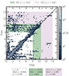 |
Fig. A.1. Comparison between LePHARE two photo-z estimates, one being the median of the probability distribution function, zPDF, and the other the redshift of minimum χ2, zchi2. All cleaning steps are applied here except for the z ≥ 8 extensive selection described in Sect. 2.2.2. The median and standard deviation of the difference zPDF − zchi2 are shown. |
Appendix B: Number counts and HOD best-fit parameters for each galaxy sample
Table B.1 shows the number of sources, number densities, best-fit HOD parameters, and model-derived quantities, for each redshift and stellar mass-limited galaxy sample.
Number of galaxies for each redshift and mass threshold bins (after cleaning); HOD best-fit parameters and model-derived properties.
Appendix C: Cross-correlations between redshift bins
To assess potential contamination in our analysis arising from photo-z estimates or source detection, we computed cross-correlations between galaxy samples at various redshift bins but with the same mass thresholds. This approach has been generalised by Szapudi & Szalay (1998), where the ACF w1, 2 between a sample D1 and a sample D2 is written as:
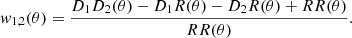 (C.1)
(C.1)
Cross-correlation analyses have been utilised in previous studies, such as Coupon et al. (2015), who employed them to validate and improve photo-z estimates, while others, like Hatfield & Jarvis (2017), used them to trace different galaxy populations. In our case, in the light of recent JWST findings that have initially identified sources as very high-z that turned out to be dusty sources around z = 3, we utilised cross-correlations to investigate how different selections for high-redshift galaxies impacted their clustering and the potential contamination from lower redshift bins. Results are presented in Fig. C.1, where all cross-correlations with the various redshift bins are shown, and for different galaxy masses. We also show in Fig. C.2 the median ratios between auto- and cross-correlations for each redshift bin, split for galaxies with log(M⋆/M⊙)≥9 and log(M⋆/M⊙)≥10.
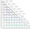 |
Fig. C.1. Cross-correlations between all redshift bins in our analysis, for each mass-limited sample. To facilitate comparisons, the autocorrelation signal for the redshift bin in each row is also shown in gray. |
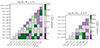 |
Fig. C.2. Median ratio between the auto- and the cross-correlations with distinct redshift bins, averaged across all angular scales, and for two stellar mass thresholds (left and right panels). Only positive values of the correlation function are taken into account here; therefore, NaN values arise when the cross-correlation is < 0. |
Notably, the large probability distributions of photo-z estimates become apparent when comparing adjacent bins, indicating potential contamination. Additionally, distinct features emerge in cross-correlations between high-redshift bins (10.5 ≤ z < 14) and lower bins (2 ≤ z < 3 or 3 ≤ z < 4.5), as well as for rare massive galaxies at z ≥ 6 or z ≥ 8. These observations suggest that even after our cleaning efforts and visual inspections, certain sources may still contaminate our high-z sample, such as highly dust-obscured galaxies or AGNs at lower z. Despite these challenges, we maintain confidence in our autocorrelation measurements, as the observed signals are about one order of magnitude lower.
Appendix D: Theory and HOD fits with nonlinear scale-dependent halo bias.
According to Jose et al. (2016), the fitting function for the nonlinear scale-dependent correction term ζ(r, Mh, z), applied to the large-scale halo bias, can be expressed as:
![Mathematical equation: $$ \begin{aligned} \zeta (r, M_{\rm h}, z)&= \zeta (\xi _{\rm mm}, \nu , \alpha _{\rm m}, M_{\rm h}) \\&= \left[ 1 + K_0 \log \left( 1 + \xi _{\rm mm}^{k_1}(r) \right) \; \nu ^{k_2} \; (1 + k_3/\alpha _{\rm m}) \right] \nonumber \\&\times \left[ 1 + L_0 \log \left( 1 + \xi _{\rm mm}^{l_1}(r) \right) \; \nu ^{l_2} \; (1 + l_3/\alpha _{\rm m}) \right] . \nonumber \end{aligned} $$](/articles/aa/full_html/2025/10/aa53828-25/aa53828-25-eq394.gif) (D.1)
(D.1)
Here, ξmm is the matter autocorrelation, ν(Mh, z) = δc/σ(Mh, z) is the peak height of halos (measurement of the “rarity” of halos), σ(Mh, z) is the variance of the linear matter overdensity field on a halo mass scale M and δc = 1.686 is the critical overdensity for halo spherical collapse. Parameters are fitted using the MS-W7 simulation, in the range 3 ≤ z < 5, as K0 = −0.0697, k1 = 1.1682, k2 = 4.7577, k3 = −0.1561, L0 = 5.1447, l1 = 1.4023, l2 = 0.5823, and l3 = −0.1030. The effective power law index αm is given by :
![Mathematical equation: $$ \begin{aligned} \alpha _{\rm m}(z) = \frac{\log (\delta _{\rm c})}{\log [M_{\rm h, nl}(z)/M_{\rm h,col}(z)]} , \end{aligned} $$](/articles/aa/full_html/2025/10/aa53828-25/aa53828-25-eq395.gif) (D.2)
(D.2)
where Mh, nl is the mass scale when the peak height equals δc, and Mh, col is the collapse mass scale when the peak height equals one. This nonlinear term in the bias goes to unity at large scales.
Figure D.1 shows the clustering measurements at z ≥ 2.5 with fitted HOD models that assume a nonlinear scale-independent halo bias from Jose et al. (2016), noted as NL-SD. These models are discussed in Sect. 4.1.3.
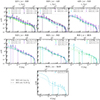 |
Fig. D.1. Angular autocorrelation function of galaxies in the COSMOS-Web survey, in redshift and mass limited bins. Dash-dotted lines show the HOD best-fit models with Jose et al. (2016) nonlinear scale-dependent halo bias, and solid lines are HOD best-fit models without it (assuming a large-scale bias of Tinker et al. 2010). |
Appendix E: Description of the simulations
Table E.1 provides a non-exhaustive overview of the simulations used in Sect. 5.2.2 to compare with our measured SHMR. In each simulation, we selected central galaxies as those hosted by the primary subhalo in each Friends-of-Friends group, defined as the subhalo with the largest number of bound particles, typically the most massive. To match the halo masses returned by our HOD model in halomod, which uses virial halo masses (total mass enclosed within a spherical overdensity as defined by Bryan & Norman 1998), we adopted the same mass definition for THESAN and Firstlight. For HORIZON-AGN, OBELISK, and TNG100, the halo mass represents the total dark matter mass in the group. Stellar mass for central galaxies is defined as the sum of all stellar particles within twice the stellar half-mass radius in TNG100, or the total mass of all bound stellar particles in the substructure for the other simulations. Where necessary, we converted these masses to a Chabrier (2003) IMF.
Non-exhaustive summary of the hydrodynamical simulations used in this work.
All Tables
Stellar mass lower thresholds in units of log(M⋆/M⊙) corresponding to MUV upper thresholds, derived by matching cumulative numbers of galaxies in our sample as a function of both properties.
Number of galaxies for each redshift and mass threshold bins (after cleaning); HOD best-fit parameters and model-derived properties.
All Figures
|
Fig. 1. Top: Galaxy number counts for COSMOS-Web and PRIMER-COSMOS, along with a fitted power law in the range 23.0 ≤ mF444W ≤ 27.0 (dashed line). Errors are computed according to Poisson noise only. Bottom: Magnitude completeness for COSMOS-Web and PRIMER-COSMOS, defined respectively as the ratio of number counts in COSMOS-Web over PRIMER-COSMOS and as the number counts in PRIMER-COSMOS over the fitted power law. The dotted black line shows the magnitude cut for COSMOS-Web where completeness falls to 80%, used for this work. |
| In the text | |
|
Fig. 2. Stellar mass distribution as a function of redshift of COSMOS-Web sources, with the mass completeness limits for COSMOS-Web in green (with errors calculated as the M⋆lim values that correspond to 85 or 95% of galaxies) and COSMOS2020 in blue as given in Weaver et al. (2022). All galaxies after magnitude filtering only are shown. Redshift bins and stellar mass thresholds, used for clustering measurements, are also represented in solid purple lines. |
| In the text | |
|
Fig. 3. Numbers of galaxies in our two highest redshift bins after the different cleaning steps applied one after the other. The top bar (dark colors) represents galaxies selected by zPDF and the bottom bar (light colors) by zchi2. |
| In the text | |
|
Fig. 4. Stack of PDF(z) in our two highest redshift bins for galaxies selected by zPDF and/or zchi2. Thin lines indicate stacks of 15 galaxies and solid lines are stacks of 50 galaxies. |
| In the text | |
|
Fig. 5. Redshift distributions for galaxies above the stellar mass completeness limit in the redshift bins chosen for this work. |
| In the text | |
|
Fig. 6. Angular autocorrelation function of galaxies in the COSMOS-Web survey, in redshift and mass limited bins. Solid lines show the HOD best-fit models, with their 1σ uncertainties in shaded regions. For the two highest redshift bins, both conservative and extended samples are represented, with HOD best-fit models in dashed and solid lines, respectively. |
| In the text | |
|
Fig. 7. Comparison of COSMOS-Web’s ACF with literature measurements (Barone-Nugent et al. 2014; Harikane et al. 2018; Cowley et al. 2018; Shuntov et al. 2022; Dalmasso et al. 2024a). Some works used UV magnitude-limited samples or LBG samples, so direct comparison with mass-limited samples is not possible. However, we chose to represent them since they are the only existing clustering measurements at z ≥ 8. |
| In the text | |
|
Fig. 8. ACF of galaxies in the bin 6 ≤ z < 8, and HOD best-fit models with and without a nonlinear scale-dependent halo bias (shown in dash-dotted and solid lines, respectively). Relative errors are presented in the bottom panel. |
| In the text | |
|
Fig. 9. Redshift evolution of the characteristic halo masses fitted in the HOD model for stellar mass-limited galaxy samples. Mh, min is the characteristic halo mass to host a central galaxy, Mh, 1 to host a satellite. Error bars are the 1σ uncertainties from the MCMC sample distribution, and quantities are shown for HOD models with and without nonlinear scale-dependent halo bias, respectively in dash-dotted and solid lines. |
| In the text | |
|
Fig. 10. Stellar-to-halo mass relationship in COSMOS-Web determined by HOD fitting of our clustering measurements. The integrated star formation efficiency is also shown from εSF = M⋆/(Mhfb). The point at 10.5 ≤ z < 14 is represented in dotted lines because it is considered less certain. Top: SHMR defined as the ratio M⋆,th/Mh,min. Bottom: SHMR defined M⋆,med/Mh,min (solid lines). It is split into two panels, z < 3 in the bottom left, and z ≥ 3 in the bottom right. The SHMR computed by abundance matching from Shuntov et al. (2025b) is also shown in dashed lines. |
| In the text | |
|
Fig. 11. Redshift evolution of the HOD-derived satellite fraction for mass-limited samples of galaxies. The point at 10.5 ≤ z < 14 is represented in dotted lines because it is considered less certain. |
| In the text | |
|
Fig. 12. Evolution of the galaxy bias with redshift, for different stellar mass thresholds, derived from the HOD modeling of our clustering measurements. The point at z ∼ 12 is represented in dotted lines because it is considered less certain. Predictions of the galaxy bias as a function of UV magnitude by Muñoz et al. (2023) and Gelli et al. (2024) are superposed, with and without implementation of a large scatter in the MUV − Mh relationship to explain the overabundance of bright galaxies at high-z. Literature measurements from McCracken et al. (2015), Harikane et al. (2016), and Cowley et al. (2018) are shown in colors corresponding to their sample threshold mass. The exception is Dalmasso et al. (2024b), which is in gray, since it corresponds to a stellar mass that is below our bin minimum. |
| In the text | |
|
Fig. 13. Evolution of the ratio between star formation rate and halo mass accretion rate as a function of redshift, in the semi-empirical model UNIVERSEMACHINE. In halo mass bins of width 0.25 dex, the ratio is computed as the halo accretion rate from the analytical formula in Behroozi et al. (2013) formula over the median SFR of galaxies hosted by halos in the mass bin. A transition in the ratio behavior is observed at a mean redshift |
| In the text | |
|
Fig. 14. Comparison of the observational SHMR in COSMOS-Web with results from various hydrodynamical simulations and the semi-empirical model UNIVERSEMACHINE. Solid lines represent the observational SHMR M⋆,th/Mh,min, obtained from HOD fitting of mass-limited galaxy clustering measurements in COSMOS-Web. The point at 10.5 ≤ z < 14 is represented in dotted lines because it is considered less certain. The dashed and other lines represent the SHMR in the simulations computed similarly to the observations, where Mh, min is the halo mass at which 50% of halos host a central galaxy with a stellar mass above M⋆,th. Top left: SHMR from TNG100 simulation snapshots, computed at the mean redshifts of each observational redshift range. Top right: SHMR from Horizon-AGN light-cone, calculated over the same redshift ranges as the observations, but limited to z ≤ 6. Bottom right: Same from UNIVERSEMACHINE light-cone in the COSMOS field, matching the observational redshift ranges. Bottom left: Same for high-z simulations (THESAN-1, FirstLight, OBELISK), computed from snapshots at mean redshifts from z ∼ 5 to z ∼ 12. |
| In the text | |
|
Fig. A.1. Comparison between LePHARE two photo-z estimates, one being the median of the probability distribution function, zPDF, and the other the redshift of minimum χ2, zchi2. All cleaning steps are applied here except for the z ≥ 8 extensive selection described in Sect. 2.2.2. The median and standard deviation of the difference zPDF − zchi2 are shown. |
| In the text | |
|
Fig. C.1. Cross-correlations between all redshift bins in our analysis, for each mass-limited sample. To facilitate comparisons, the autocorrelation signal for the redshift bin in each row is also shown in gray. |
| In the text | |
|
Fig. C.2. Median ratio between the auto- and the cross-correlations with distinct redshift bins, averaged across all angular scales, and for two stellar mass thresholds (left and right panels). Only positive values of the correlation function are taken into account here; therefore, NaN values arise when the cross-correlation is < 0. |
| In the text | |
|
Fig. D.1. Angular autocorrelation function of galaxies in the COSMOS-Web survey, in redshift and mass limited bins. Dash-dotted lines show the HOD best-fit models with Jose et al. (2016) nonlinear scale-dependent halo bias, and solid lines are HOD best-fit models without it (assuming a large-scale bias of Tinker et al. 2010). |
| In the text | |
Current usage metrics show cumulative count of Article Views (full-text article views including HTML views, PDF and ePub downloads, according to the available data) and Abstracts Views on Vision4Press platform.
Data correspond to usage on the plateform after 2015. The current usage metrics is available 48-96 hours after online publication and is updated daily on week days.
Initial download of the metrics may take a while.