| Issue |
A&A
Volume 702, October 2025
|
|
|---|---|---|
| Article Number | A197 | |
| Number of page(s) | 13 | |
| Section | Stellar structure and evolution | |
| DOI | https://doi.org/10.1051/0004-6361/202554162 | |
| Published online | 21 October 2025 | |
Spindown of massive single main sequence stars in the Milky Way
1
Argelander-Institut für Astronomie, Universität Bonn, Auf dem Hügel 71, 53121 Bonn, Germany
2
Center for Computational Relativity and Gravitation, Rochester Institute of Technology, Rochester, NY 14623, USA
3
Instituto de Astrofísica de Canarias, 38200 La Laguna, Tenerife, Spain
4
Departamento de Astrofísica, Universidad de La Laguna, 38205 La Laguna, Tenerife, Spain
5
European Southern Observatory, Alonso de Córdova 3107, Vitacura, Santiago, Chile
⋆ Corresponding author: This email address is being protected from spambots. You need JavaScript enabled to view it.
Received:
17
February
2025
Accepted:
22
July
2025
Abstract
Context. We need to understand the spin evolution of massive stars to compute their internal rotation-induced mixing processes, isolate effects of close binary evolution, and predict the rotation rates of white dwarfs, neutron stars, and black holes.
Aims. We discuss the spindown of massive main sequence stars imposed by stellar winds.
Methods. We used detailed grids of single-star evolutionary models to predict the distribution of the surface rotational velocities of core hydrogen-burning massive Galactic stars as function of their mass and evolutionary state. We then compared the spin properties of our synthetic populations with appropriately selected subsamples of Galactic main sequence OB-type stars extracted from the IACOB survey.
Results. We find that observations and models agree that the surface rotational velocities of massive Galactic stars below ∼40 M⊙ remain relatively constant during their main sequence evolution. The more massive stars in the IACOB sample appear to spin down less strongly than predicted, while our updated angular momentum loss prescription predicts a faster spindown. Furthermore, the observations show a population of fast rotators, v sin i ≳ 200 km s−1, persisting for all ages. This is not reproduced by our synthetic single star populations.
Conclusions. We conclude that the wind-induced spindown of massive main sequence stars is yet to be fully understood. In this regard, lower stellar wind mass-loss rates than we used here might alleviate the discrepancy between observations and predictions at higher masses, but would likely not solve it. We propose that binary evolution might significantly contribute to the fraction of rapid rotators in massive stars.
Key words: stars: evolution / stars: massive / stars: rotation
© The Authors 2025
 Open Access article, published by EDP Sciences, under the terms of the Creative Commons Attribution License (https://creativecommons.org/licenses/by/4.0), which permits unrestricted use, distribution, and reproduction in any medium, provided the original work is properly cited.
This article is published in open access under the Subscribe to Open model. This email address is being protected from spambots. You need JavaScript enabled to view it. to support open access publication.
1. Introduction
Rotation plays a key role for the whole evolution of massive stars, from their birth to the formation of their end products. Models indeed predict that it may have an impact as strong as their initial mass or metallicity (Meynet & Maeder 2000; Langer 2012; de Mink et al. 2013). As a massive star evolves, its surface equatorial velocity is influenced by several factors. Massive single stars typically spin down as a result of the coupling of angular momentum loss by stellar winds and efficient internal transport of angular momentum (Langer 1998). This is not true for stars in binary systems, where interactions such as mass transfer can cause the rotation rate of a star a star to increase or decrease (e.g., Zahn 1975; Packet 1981; Petrovic et al. 2005; de Mink et al. 2013).
To understand stellar rotation, the projected rotational velocities (v sin i) need to be derived from spectroscopic data (e.g., Conti & Ebbets 1977; Penny 1996; Huang et al. 2010; Zorec & Royer 2012; Ramírez-Agudelo et al. 2013; Markova et al. 2014; Simón-Díaz & Herrero 2014; Dufton et al. 2019; Daher et al. 2022; Sun & Chiappini 2024) and the effect of rotation on the stellar structure and evolution must be studied. The former can be used to constrain the distribution of the initial rotation rate (Rosen et al. 2012; Holgado et al. 2022), investigate the spins of evolved magnetic stars (Fossati et al. 2016; Petit et al. 2019; Keszthelyi et al. 2020), study rotationally induced mixing and chemically homogeneous evolution (Yoon & Langer 2005; Martins et al. 2013, 2017; Markova et al. 2018), probe angular momentum loss (Granada & Haemmerlé 2014; Rieutord & Beth 2014; Gagnier et al. 2019), diagnose magnetic braking (Meynet et al. 2011; Curtis et al. 2019; Hall et al. 2021; David et al. 2022), assess theories of massive star formation (Wolff et al. 2006; Mokiem et al. 2006; Huang et al. 2010; Chiappini et al. 2011), and constrain the rotation rates of the final compact objects (Heger et al. 2000; Petrovic et al. 2005). Most work on stellar wind mass loss, including this paper, has been done with one-dimensional (1D) models, but rapidly rotating stars are distorted from spherical symmetry through centrifugal forces and because the flows across and in the star are two-dimensional (2D; Friend & Abbott 1986; Pelupessy et al. 2000; Müller & Vink 2014; Hastings et al. 2023), which in the end also affects the stellar observables (Abdul-Masih 2023).
Stars are generally thought to be born spinning rapidly, due to the large angular momentum content of their birth clouds. While solar-type stars spin down dramatically as a result of the coupling of their winds with their convection-generated magnetic fields (Skumanich 1972; David et al. 2022), massive main sequence (MS) stars, on the other hand, are thought to spin down much less strongly, even though their winds are stronger by many orders of magnitude. In addition to their short lifetimes, they generally do not have large-scale surface magnetic fields. The few percent of massive MS stars with observed magnetic fields spin down strongly (Fossati et al. 2016; Petit et al. 2019).
In nonmagnetic massive single stars, the evolution of their surface rotation velocity during the MS is affected by: (i) the expansion during the MS, (ii) the redistribution of internal angular momentum, and (iii) angular momentum loss due to winds. Massive stars on the MS expand by a factor of ≈3, for which angular momentum conservation would imply a corresponding spindown of the stellar surface. The envelope expansion is accompanied by simultaneous core contraction and efficient transport of the resulting excess angular momentum from the core to the envelope (Ekström et al. 2008; Brott et al. 2011; de Mink et al. 2013). These two processes have opposite effects on the surface rotation, with the latter being more relevant for massive stars because their core mass fraction is larger (Hastings et al. 2020).
Nonmagnetic stars also lose angular momentum when they undergo stellar wind mass loss. In a simplified picture of spindown due to stellar winds, the mass that is removed by stellar winds also contains angular momentum. The new surface layers expand and would spin down if their angular momentum were conserved. Shear induces angular momentum transport toward reestablishing rigid rotation, however, so angular momentum from deep inside is brought toward the surface of the star. The net effect is a spindown of the whole star. The dominant effect of a stellar wind on a nonmagnetic rotating star is indeed angular momentum loss rather than mass loss, as the relative rate of angular momentum loss exceeds that mass loss by one order of magnitude (Langer 1998). On the MS, the winds are stronger at higher masses and higher metallicities (e.g., Kudritzki & Puls 2000; Mokiem et al. 2007). For massive Milky Way stars, angular momentum loss is expected to strongly affect spindown for MS stars above ∼9 M⊙ (Langer 2012).
We extend the work of Holgado et al. (2022) to investigate the spindown of massive Galactic stars across the MS. We predict the distribution of the surface rotational velocities of MS massive Galactic stars based on this simple picture, and compare them to the observed evolution of the rotation rate as obtained from the IACOB survey (Simón-Díaz et al. 2011, 2020). In Sect. 2 we discuss our evolutionary models and describe the population synthesis algorithm we developed. In Sect. 3 we analyze the spindown evolution of our models. In Sect. 4 we discuss the sample of observed stars. In Sect. 5 we compare the distributions of the projected rotational velocity of the observed stars and the synthetic populations with two different angular momentum prescriptions. In Sect. 6 we discuss the uncertainties in our methods and the observed sample. We provide a brief summary in Sect. 7.
2. Method
We used the Galactic metallicity evolutionary models of Brott et al. (2011) to derive predictions for the evolution of the surface rotational velocity of massive stars across the MS. We first describe the essential physics assumptions in these models, then discuss the assumptions on stellar wind-induced angular momentum loss. We do this for the original models, and we describe how, based on the data from the original models, we used a newly devised prescription for angular momentum loss. Furthermore, we explain the way in which we used the model data to derive a synthetic population of massive stars in order to predict the expected distribution of the rotational velocities.
2.1. Evolutionary models
We used the Galactic single-star evolutionary models from Brott et al. (2011), henceforth referred to as the Brott models. The grid has a mass range from 3 M⊙ to 100 M⊙, of which the models of 80 M⊙ and 100 M⊙ were computed after the paper by Brott et al. (2011). was published, but with exactly the same code, physics ingredients, and input parameters. It contains models with initial equatorial rotational velocities from 0 km s−1 to 550 km s−1. The models are calculated with the 1D stellar evolution code described by Heger et al. (2000), Petrovic et al. (2005), and Yoon & Langer (2005). The initial mass fractions of hydrogen, helium, and metals are Xi = 0.7274, Yi = 0.2638, and Zi = 0.0088. We note that despite the low overall metallicity, which is due to the low solar oxygen abundance suggested by citeAsplund et al. (2005), the models are well suited to describe massive Galactic stars, because their mass-loss rate as well as their opacity is based on the adopted iron abundance (cf. Sect. 2.3 in Brott et al. 2011).
The major physics assumptions are as follows (a more detailed discussion is provided in Brott et al. 2011). Mixing and angular momentum transport are treated as diffusive processes. Angular momentum transport is dominated by the Spruit-Tayler dynamo (Spruit 2002). Magnetic fields keep the star near rigid rotation while on the MS. This suppresses shear mixing between layers.
Convection uses the standard mixing length theory (MLT) as described by Cox & Giuli (1968) and is modeled with the Ledoux criterion with a mixing length parameter αMLT = 1.5. Semi-convection follows the prescription of Langer et al. (1983) and uses the semi-convection parameter αSEM = 1. Convective core overshooting uses a parameter of 0.335 multiplied by the pressure scale height.
Stellar wind mass loss is calculated with the prescriptions of Vink et al. (2000, 2001), which is based on the method described by de Koter et al. (1997), as well as the recipes from Hamann et al. (1995) and Nieuwenhuijzen & de Jager (1990). These two prescriptions predict strong mass loss at the bistability jumps found at Teff ∼ 22 kk and Teff ∼ 12.5 kk. Notably, the mass-loss rates in the Brott models are scaled directly with the adopted iron abundance, not with the overall metallicity, and they are therefore not affected by the adopted oxygen abundance. The Brott models adopt a rotationally induced mass-loss enhancement, which becomes relevant for models near critical rotation.
As discussed in Sect. 1, rapid rotation deforms stars and is difficult to model in a 1D code. We calculated the stellar structure equations and stellar properties on isobaric mass shells. This enforced the shellular approximation, which assumes that the angular velocity is constant on isobaric surfaces that correspond to mass shells. Centrifugal acceleration was accounted for with the methods of Endal & Sofia (1976) and Kippenhahn & Thomas (1970). The critical velocity was calculated as  , with ΓEdd = L/LEdd as the Eddington factor and LEdd as the Eddington luminosity.
We defined the zero-age main sequence (ZAMS) as the point where 5% of the initial core hydrogen mass fraction has been burned. For models with an initial mass of 35 M⊙ and below, we defined the terminal-age main sequence (TAMS) as the beginning of the MS hook, which is the point at which core hydrogen has been exhausted and the stellar core contracts to raise the temperature in preparation for helium burning, which also raises the effective temperature (Teff). Above this initial mass the models do not show a MS hook because stellar winds blow off the envelope before the end of the MS. For these models, we defined TAMS as when the core hydrogen mass fraction drops to 0.03.
We derived model predictions for the spin evolution in two ways. First, we used the original data from the Brott models. Because a new method for calculating the angular momentum loss was devised recently (see Sect. 2.2), we developed a new prescription for the angular momentum loss, which was then used to derive a new prediction for the spin evolution.
2.2. Angular momentum loss
In the Brott models, the amount of angular momentum that is lost due to stellar winds ΔJ over one timestep Δt is computed by simply removing the angular momentum contained in the outermost layer of mass ΔM that is lost during the timestep, that is, by integrating the specific angular momentum profile, j(m), as
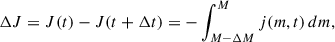 (1)
(1)
where m is the Lagrangian mass coordinate, and the removed mass is  for the specified stellar wind mass-loss rate Ṁ. In a rigidly rotating star, Eq. (1) may lead to an underestimate of the angular momentum loss, which we can see as follows.
The time resolution of the evolutionary models is such that variations in the stellar surface properties over one timestep are small. In particular, for a significant mass-loss rate, the difference in stellar radius of two successive models is small compared to the difference between the stellar radius and, in the same stellar model, the radius of the mass coordinate that defines the surface after the next timestep.
When we assume that the star remains in rigid rotation, and neglect the change in stellar radius, mass-loss rate, and surface specific angular momentum jsurf during one timestep, a more accurate way to compute the angular momentum loss is (cf., Paxton et al. 2019)
 (2)
(2)
Both approaches assume that mass flux is independent of latitude, and that j(m) and jsurf are averaged over latitude assuming rigidly rotating shells (Heger et al. 2000).
Figure 1 illustrates the difference in the amount of angular momentum that is removed by both prescriptions. Our new prescription (Eq. (2)) is more correct than the previous prescription (Eq. (1)) when the star keeps its angular momentum profile (e.g., rigid rotation), because in this case, the layer marked by R1 has the same specific angular momentum at time t + Δt as the layer marked by R2 at time t. The prescription originally implemented in the Brott models results in the loss of a smaller amount of angular momentum, by a fraction that depends on the mass-loss rate and timesteps used in the calculations. Notably, for very small changes in mass per timestep, the two prescriptions remove essentially the same amount of angular momentum.
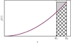 |
Fig. 1. Schematic diagram of the specific internal angular momentum j of a model as a function of radius coordinate r, illustrating the angular momentum loss prescriptions corresponding to Eqs. (1) and (2). The width of the hatched area indicates the radius range that contains the material that is removed from the model within one timestep, where R2 corresponds to the stellar surface of the considered model, and R1 marks the layer that becomes the stellar surface after the next timestep. The prescription implemented in the Brott models removes the angular momentum represented by the hatched area. The new prescription removes the angular momentum in the hatched plus the shaded area. |
While the angular momentum loss should not depend on the timestep of the numerical calculations, the difference between the old and our new prescription may reflect the magnitude of the uncertainty of the angular momentum loss predicted by our 1D stellar evolution models. Our new approach may be formally more correct, but it depends on the assumption that the outer stellar layers remain essentially rigidly rotating.
The evolution of stars is essentially independent of their initial rotation velocity for the range of rotation rates in this paper. As shown by Brott et al. (2011), the models of the same mass and different initial rotational velocity follow essentially the same evolutionary tracks until a threshold velocity, above which the models evolve chemically homogeneously off the ZAMS. For Galactic metallicity, this threshold velocity is near vrot, i ≃ 500 km s−1 up to 50 M⊙. For higher masses, homogeneous evolution may ensue at lower initial rotational velocities, but if it does, it only lasts for a short time, because these models spin down very rapidly (see Fig. 3 in Sect. 3 below). Because that the initial velocity distribution we derived from the observational sample (Sect. 4.2) drops sharply near vrot, i ≃ 100 km s−1, and 1% of all stars are above vrot, i ≃ 400 km s−1, we considered it simple and accurate to apply the new prescription for angular momentum loss to the Brott models. We used Eq. (2) to recalculate the rate of angular momentum loss in the Brott models and used the results to compute revised values for J, jsurf, and vrot.
2.3. Population synthesis
We developed the population synthesis algorithm Hōkū (Nathaniel 2022, available on request) in order to study the statistical properties of single MS stars. When the appropriate distribution functions are used, Hōkū takes a specified initial mass (mi), ZAMS rotational velocity (vZAMS), and age (τ*) and selects four model stars from the grid. The algorithm then interpolates stellar parameters from these four tracks, using a three-dimensional linear interpolation algorithm. This process is repeated many times until Hōkū has interpolated a population of sufficient size.
Hōkū interpolates a simulated star as follows: After drawing mi, vZAMS, and τ*, it selects the two closest initial masses above and below mi in the model grid. For each of these masses, Hōkū then selects the two model stars with ZAMS velocities above and below vZAMS. These four models are used in interpolation. The rotational velocity of a model can change between the beginning of the simulation and ZAMS, especially for massive stars. Hōkū therefore uses the ZAMS velocity of the models and not their initial velocity.
The MS lifetime (τMS) depends on the initial mass and the rotation rate. The four models are therefore not necessarily in the same evolutionary stage at the same age. To compensate for this, we used the fractional MS age, fMS = τ*/τMS, as the interpolation variable, and not just τMS. Hōkū interpolates an MS lifetime for the simulated star from the MS lifetimes of the four model stars and uses this to determine fMS of the simulated star. If fMS > 1, however, the simulated star is thrown out and Hōkū moves to the next initial parameter set. This ensures that the population consists of simulated MS stars alone.
When this process is complete, Hōkū can interpolate observables for the simulated star from the four stellar models. In addition to population synthesis, Hōkū can also calculate isochrones and evolutionary tracks. A visual representation of the interpolation process and an interpolated evolutionary track is shown in Fig. 2.
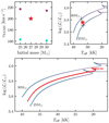 |
Fig. 2. Top: Illustration of the Hōkū interpolation process. The left panel shows the initial masses and ZAMS velocities of the grid models in purple and turquoise, and the simulated star is shown in red. The right panel shows the evolutionary models in a spectroscopic HR diagram and the interpolated effective temperature and spectroscopic luminosity of the simulated star. The crosses mark where the effective temperature and spectroscopic luminosity are interpolated from the grid models. Bottom: Resulting evolutionary track of the 27 M⊙, |

3. Model predictions
Figure 3 shows the MS evolution of the surface rotation velocity of the Brott models from 10 M⊙ to 100 M⊙ based on our new predictions. The lines converge with time (or with burned hydrogen fraction) in all panels. This mainly occurs because the rate of angular momentum loss is proportional to the surface specific angular momentum, which implies that faster rotators spin down faster than slower rotators. In addition, the spindown distinctly depends on the initial mass of the stars, because the mass depends on the three processes that affect spin evolution we described in Sect. 1: expansion, internal transport, and mass loss.
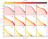 |
Fig. 3. Evolution of the rotational velocity from ZAMS to TAMS of Brott models according to the new predictions (derived as discussed in Appendix A). Each panel shows a different initial mass, and the colors indicate the effective temperature over the course of the MS. The x-axis shows the current core hydrogen mass fraction (Xcore) divided by the initial core hydrogen mass fraction (Xcore, i). |
In the mass range 10 − 20 M⊙, the core mass fractions are larger. Their contraction triggers an angular momentum flow from the core into the envelope, which significantly contributes to counteracting the spindown of the surface layers (see Hastings et al. 2020 for an in-depth discussion). In particular, the 12 M⊙ and 15 M⊙ models even show a spinup during the first part of their hydrogen-burning evolution. Stars are rarely born with a very high rotation rate (Bodenheimer 1995), and the majority of stars in this mass range are therefore predicted to evolve with a nearly constant rotational velocity over most of their hydrogen-burning lifetime. The mass-loss effect also kicks in in this mass range, however, especially during the second half of the MS evolution, during which the stars are on the cool side of the wind bistability regime where the mass-loss rates are significantly higher (cf. Vink et al. 2010, although some new evidence may refute this, see e.g., de Burgos et al. 2024).
For stars above ∼25 M⊙, mass loss dominates the spin evolution from the beginning, and the mass-loss-induced spindown is so strong that all models end their core-hydrogen burning with surface rotation velocities near zero. As the effect becomes stronger with mass, the most massive stars considered here, with a mass above ∼50 M⊙, reach this situation during core hydrogen-burning and live a significant fraction of it essentially without rotation. This effect is augmented by the envelope inflation of the models near their Eddington limit for masses above ∼30 M⊙. (Sanyal et al. 2015, 2017)
Although in Fig. 3 we only present results for the spin rate evolution with our new prescription for angular momentum loss, it is interesting to briefly mention the main effects of considering either prescription. In Appendix A we present a comparison between the two prescriptions for the total angular momentum, the surface specific angular momentum, and the rotational velocity quantities.
Below ∼10 M⊙, the mass-loss effect is small, and our new results are very close to the original prediction of the Brott models. Even at 20 M⊙, the difference for a model that initially rotates with about 200 km s−1 remains within a few percent (see Fig. A.1). For higher masses, however, the difference quickly becomes more appreciable. Considering stars that initially rotated with about 200 km s−1, we found that they spin down completely, while the original Brott model spins down to about 80 km s−1. The difference between the original and our new calculation is largest at the top end of the considered mass spectrum. In the original calculations, the 100 M⊙ model starting with ∼200 km s−1 spins down to 135 km s−1 when half of the hydrogen is burned in the center, while it reaches ∼50 km s−1 with our new approach at the same moment in time. Complete spindown (vrot < 10 km s−1) is reached at a core hydrogen mass fraction of 0.14 compared to 0.30, respectively.
4. Observational sample and preprocessing
The observations we used come from a subsample of the stars for which the IACOB project (Simón-Díaz et al. 2011, 2020) have compiled high-quality spectroscopic observations. In particular, we focused on the samples of O stars and B-type supergiants that were described and spectroscopically analyzed by Holgado et al. (2020, 2022) and de Burgos et al. (2023, 2024), respectively. These are about 800 massive Galactic stars.
As described in the papers mentioned above, the samples we considered exclude all stars that were classified as double-line spectroscopic binaries (SB2) and only concentrated on stars that were identified as likely single stars and single-line spectroscopic binaries (SB1). While eliminating the SB2 seems appropriate for the comparison to single-star population synthesis, we remark that following de Mink et al. (2013), a non-negligible percentage of the remaining sample of stars that were categorized as apparently single and SB1 might be the outcome of a binary interaction event.
Throughout the paper, we use the spectroscopic Hertzsprung-Russell diagram (sHRD; ℒ ≡ Teff4/g with g as surface gravity; Langer & Kudritzki 2014) to compare our results with the observed stars. This eliminates uncertainties in reddening and distance.
4.1. Kernel density estimate
We compared the observed stars to the synthetic populations by constructing a 2D kernel density estimate (KDE) for each observed star in the sample, placed in the spectroscopic Hertzsprung-Russell diagram, and normalizing it so that the sum was unity (obtaining the full sample KDE is simply a matter of adding the individual KDEs). The uncertainties in Teff and ℒ were used as the standard deviations in the KDEs. Integration of the KDE of an individual star over an arbitrary area on the sHRD gives the probability that the star is located in this area, and therefore, the weight it should be given in constructing a distribution of the stellar parameter in question. Accordingly, every star was considered when we constructed distributions, but the magnitude of the contribution of any given star (the weighting factor) varied based on its location relative to the chosen area in the sHRD.
Summing these weighting factors resulted in a number, not necessarily an integer, to which the data can be considered equivalent. A distribution that sums to 10, for instance, might consist of data from 5 stars that each have a weighting factor of 20%, or 100 stars that each have a weighting factor of 10%. This method allowed us to construct distributions for selected portions of the sHRD while taking observational uncertainties into account. We did not introduce any smoothing, and we conversely did not attempt to deconvolve our observational errors. The result is shown in Fig. 4.
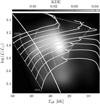 |
Fig. 4. 2D KDE of the entire observed sample in the sHRD (background). The solid lines show the evolutionary tracks of Brott models at 20 M⊙, 25 M⊙, 30 M⊙, 35 M⊙, 40 M⊙, 50 M⊙, 60 M⊙, 80 M⊙, and 100 M⊙ with an initial rotational velocity of 200 km s−1. The dotted lines divide the MS into quarters, determined by the fraction of the initial core hydrogen mass fraction that has been burned. The white line indicates log g = 3.7 dex. Only stars to the left of this line were used to create the initial velocity KDE discussed in Section 4.2. |
We used the location of the stars in the sHRD to create our comparison samples, which did not require information about measured masses. Figure 4 includes some stars with parameters below logℒ/ℒ⊙ ∼ 3.5 (paper in prep.). For the purposes of this paper, we concentrated on the stars that are located above the 20 M⊙ track.
4.2. Initial rotation velocity PDF
We chose to use the observed sample to construct an initial velocity distribution for use in our population synthesis algorithm. In order to exclude more evolved stars, we only used stars with log g > 3.7 dex in constructing our distribution (this line is marked in Fig. 4). Notably, according to the stellar models, this condition selects stars during the first half of their MS evolution, while a higher threshold surface gravity would select stars closer to the ZAMS. The number of sample stars drops quickly toward the ZAMS (Holgado et al. 2020), however, such that a higher threshold gravity would not give us enough statistics. This implies that we can only constrain the spindown evolution of massive Galactic stars in the second half of their MS evolution.
We explored two different fit methods for the data, one method in linear space, and another method in logarithmic space. For the linear space fit, we used the *|scikit-learn| GaussianMixture method (Pedregosa et al. 2011) for a two-component Gaussian. This fit accurately reproduces the feature seen at ∼200 km s−1 in the histogram, but allows for negative velocities in the PDE. For the logarithmic space fit, we first took the logarithm of the data and then fit it with the *|scipy.stats| (Virtanen et al. 2020) one-component Gaussian KDE function. The resolution of this logarithmic space fit was not high enough to capture the feature at ∼200 km s−1, but it prevents unphysical negative velocities.
The v sin i distribution of the observed sample is poorly characterized by a single Gaussian in linear or log space, and there is an overabundance in density at higher velocities relative to the single Gaussian fit. We performed a linear regression with *|scipy.stats| and found no statistically significant differences in their performance. Therefore, we chose to use the KDE fit in log space for Hōkū because it prevents negative velocities and is simpler to work with. The histogram and the two fits are shown in Fig. 5.
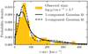 |
Fig. 5. Distribution of the projected rotational velocity for the observed stars with log g > 3.7 dex, overplotted with one- and two-component Gaussian KDEs (solid and dashed lines, respectively). |
5. Comparison with observations
In this section, we compare the observed v sin i-distributions with our theoretical predictions using Hōkū. We first considered the results taken directly from the Brott models and compared them with the IACOB data. In a second step, we compared the observational data with the v sin i distributions derived from the Brott models after we applied our new prescription for the angular momentum loss.
We used a flat initial mass function (IMF) from 20 M⊙ to 100 M⊙ and assumed continuous star formation. We drew inclination angles (i) from a PDF that assumed a random orientation cos i. We used the distribution function discussed in Sect. 4.2 to draw a vZAMS sin i for each simulated star and then divided by sin i to obtain vZAMS, which ranges from ∼1 km s−1 to ∼ 560 km s−1.
We first binned the synthetic population by initial mass using four bins of 20–30 M⊙, 30–40 M⊙, 40–60 M⊙, and 60–100 M⊙. We chose the first 20–30 M⊙ mass bin because winds are weaker in this range than in higher mass bins (Vink 2022). The other mass bins were chosen to be approximately evenly spaced in logℒ/ℒ⊙.
To facilitate seeing how rotational velocity changes with time, we divided the MS into quarters based on how much of the initial core hydrogen has been burned. For example, the first quarter consisted of simulated stars with a core hydrogen mass fraction of Xi to 0.75Xi, and the last quarter consisted of simulated stars with a core hydrogen mass fraction of 0.25Xi to TAMS. This technique allowed us to determine the mass-dependent evolution of the rotational velocity across the MS.
5.1. Comparison with the original Brott model predictions
Focusing first on the theoretical data, Fig. 6 shows an overall spindown of stars with time in all four considered mass bins. In the lowest mass bin (20–30 M⊙), the spindown is mild and barely shifts the peak of the distribution to lower v sin i values. Only the initially fastest rotators are moved substantially, such that barely any star with v sin i > 250 km s−1 is predicted. For higher masses, the predicted spindown increases markedly, with upper limits to the v sin i values of 210 km s−1, 180 km s−1, and 100 km s−1 in the last quarter of the three higher mass bins.
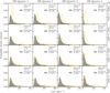 |
Fig. 6. Distributions of the projected rotational velocity, v sin i for the observed stars (yellow lines) and for the synthetic population (gray histograms), where the v sin i is calculated using the rotational velocities directly from the models of Brott et al. (2011). The four columns show the different quarters of the MS, as denoted above, and the four rows show the different mass bins, as denoted to the right. The numbers in the legends indicate the number of observed or simulated stars in the respective histograms (see Sect. 4.1). The simulated distribution reaches beyond the y-axis boundary in two panels, where for the 100–60 M⊙ mass bin, the fourth quarter reaches to 0.13, and for the 60–40 M⊙ mass bin, the fourth quarter reaches to 0.069. |
The spindown in the models of all four mass bins accelerates with time. The model histograms in the first two quarters are almost identical even in the highest mass bin. For the lower two mass bins, even the predicted distributions in the second and third quarter are nearly the same. The greatest differences in the subsequent quarters occurs between the third and the fourth and is still rather modest in the lowest mass bin (20–30 M⊙).
When we compare the predictions with the observed v sin i distributions, starting with the lowest mass bin, the agreement is good. While this is expected for the first two quarters, which contain the stars we used to design our initial v sin i distribution, it confirms that angular momentum transport from the core into the envelope of the stars must take place. The stellar radii increase by a factor of ∼2 from the second to the fourth quarter, such that local angular momentum conservation would lead to a spindown by the same factor, which is neither observed nor predicted. On the other hand, the fastest rotating models (v sin i > 200 km s−1) are spun down in the last quarter, while the number of observed fast rotators increases. While the total number of these stars is small, this effect is observed in all four mass ranges, which indicates that it is significant; we return to this below.
In the 30–40 M⊙ mass range, the situation is similar to the 20–30 M⊙ range. Here and in the higher mass ranges, the number of observed stars in the first quarter is small and the corresponding histogram is not overly meaningful. In the last two quarters, the spindown in both the observed and the model distributions is similar to the lower mass range, perhaps slightly more pronounced in the final quarter. Most notably in the fourth quarter, however, the predicted distribution is more strongly skewed toward v sin i = 0 than the observed distribution. This might imply that the angular momentum loss in the models is overestimated. On the other hand, the observed stars in the fourth quarter are giants or supergiants, which are known to be strongly affected by additional nonrotational sources of line broadening. In particular, macroturbulent and microturbulent broadening might both play a significant role in the reliability of the v sin i estimates (below a given threshold) if the relative contribution of the three broadening mechanisms is not adequately separated in the analysis of the line profile (see, e.g., detailed explanations and illustrative examples in Simón-Díaz & Herrero 2014; Simón-Díaz et al. 2017; Holgado et al. 2022). As indicated by Holgado et al. (2022) and de Burgos et al. (2023), our v sin i measurements are properly decontaminated from macroturbulent broadening, but it is possible that microturbulent broadening imposes a limit on the line-broadening analysis that our advanced methods perform to reliably reach values of v sin i below 20 km s−1 to 40 km s−1 in certain parameter domains. The reason of the mismatch between the predicted and observed number of slow rotators in the fourth quarter of the 30–40 M⊙ mass range might therefore also be associated with limitations in our availability to obtain reliable of projected rotational velocities in the low v sin i domain, as further discussed by Holgado et al. (2022, in particular, their Sect. 3.2.3 and Appendix D).
For the top two mass bins in the figure (100–60 M⊙ and 60–40 M⊙) without the first quarter, the observed distributions do not change strongly with evolutionary time. In particular, the distributions of the second and third MS quarter are very similar. This seems to imply that even at the highest considered masses, the rotational velocities do not change significantly during the first 75% of the MS evolution. This is remarkable because especially in the third quarter, the models predict a significant spindown. The discrepancy is strongest in the fourth quarter, for which the observations signify some spindown, but not as much as predicted by far. It appears to be doubtful whether this rather large discrepancy can be masked by observational limitations (imposed by macro- or microturbulence) when measuring projected rotational velocities.
5.2. Comparison with the updated Brott model predictions
We show the comparison of the IACOB data with the distributions of v sin i calculated with our new angular momentum loss approach in Fig. 7, which is structured in the same way as Fig. 6. Since the new predictions of all four panels of the lowest mass range and the predictions of the first three panels of the 30–40 M⊙ range are almost identical with those from the original Brott model data and the changes are small even in the fourth quarter of the latter mass range, we only discuss the two top mass ranges here.
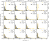 |
Fig. 7. As Fig. 6, but with v sin i values for the synthetic population calculated by applying our new angular momentum loss recipe to the models of Brott et al. (2011), as discussed in Appendix A. The simulated distribution reaches beyond the y-axis boundary in four panels. For the 60–100 M⊙ mass bin, the third quarter reaches to 0.08 and the fourth quarter reaches to 0.17. For the 40–60 M⊙ mass bin, the fourth quarter reaches to 0.12. For the 30–40 M⊙ mass bin the fourth quarter reaches to 0.05. |
The angular momentum loss according to our new prescription is larger than in the original Brott models. In particular in the 40–60 M⊙ and 60–100 M⊙ mass ranges, the predicted spindown is therefore stronger. As the spindown of the very massive original Brott models appeared to be stronger than that implied by the IACOB data, this discrepancy increases when compared to the new predictions. Already in the third MS quarter, the models cover less than half of the observed distributions in both mass ranges. In the fourth quarter, the models cover ∼5% of the observed distribution for 40–60 M⊙, and the overlap between the observed and predicted distributions is essentially zero in the highest mass bin. We conclude that our new angular momentum loss prescription overpredicts the wind-induced angular momentum loss in stellar models.
6. Discussion
From the comparisons of the model predictions with the IACOB data, we can draw the following conclusions. It appears that toward lower masses, in particular, for stars below 30 M⊙, the available predictions are not sensitive to the theoretical uncertainties. The main feature of the models is that for rotational velocities below ∼200 km s−1, which cover ≳90% of the observed stars, the rotational velocity remains rather constant throughout the MS evolution. This trend agrees well with the observed rotational velocity distributions. Unless the observed stars contain significant radial angular velocity gradients, it implies that the rotation of the expanding envelope is strongly coupled to the rotation of the contracting core.
Toward higher masses, particularly above 40 M⊙, signs of angular momentum loss are clearly visible in the observed v sin i distributions because the peak of the distribution moves to slower v sin i values as the stars progress across the MS. The data provide a vivid test of the adopted angular momentum loss in stellar evolution models. While on the grounds of physical consistency, our new prescription appears to be preferable over the prescription used in the original Brott models, it clearly overpredicts the angular momentum loss when applied to the Brott model data. While the original Brott models also lead to slower rotation than what is derived from the IACOB data, this difference might also be related to uncertainties in relation to atmospheric microturbulence in the evolved very massive stars. Regardless of the used angular momentum loss prescription, the models predict that any initially very fast rotator (vrot ≳ 200 km s−1) should have been spun down by its wind to lower velocities by the end of the MS evolution.
The continued presence of very fast rotators in samples of increasingly more evolved massive stars (MS quarters 2, 3, and 4 in Figs. 6 and 7) implies that these are unlikely to be evolved stars that were born as rapid rotators, but instead that they have been spun-up at one point during their MS evolution. This spinup is predicted by models of mass-transferring binary stars (Langer 2012; de Mink et al. 2013), and confirmed by many observations (Vanbeveren et al. 2018; Klement et al. 2019; Tauris & van den Heuvel 2023). Notably, internal gravity-mode pulsations may also produce ways to spin-up the stellar surface layer (Rogers 2015; Townsend et al. 2015).
One way to alleviate the problem of a strong spindown for stellar models above ∼40 M⊙ for a given angular momentum loss prescription would be to lower the adopted mass-loss rates. The Brott models follow the prescription by Vink et al. (2001), which includes the so-called bistability jump, a rapid increase in mass loss near Teff = 22 kk that results in a strong spindown. However, several works that derived empirical mass-loss rates in luminous OB stars have shown lower rates than the predictions of Vink et al. (2001) for Teff ≲ 25 kk (e.g., Rubio-Díez et al. 2015; Bernini-Peron et al. 2015; de Burgos et al. 2024; Verhamme et al. 2024). The adoption of both lower mass-loss rates overall and a smaller bistability mechanism may require an additional source of angular momentum loss in stars above 20 M⊙, however, to reconcile observations and predictions (Keszthelyi et al. 2017). Therefore, lower mass-loss rates below Teff ∼ 25 kk (by the bistability jump) might alleviate the increasing discrepancy between observations and predictions in the fourth MS quarter of Figs. 6 and 7, above ∼30 M⊙ (strongest in Fig. 7 based on results using the new angular momentum loss scheme). These two figures also show, however, that the spindown problem already occurs in the third MS quarter, strongest in Fig. 7 based on results using the new angular momentum loss scheme. Since faster rotators spin down faster than slower rotators (see Sect. 3), it seems unlikely that a general downward correction of the mass-loss rates by a factor of ∼2 for stars between 40 M⊙ and 100 M⊙ would be sufficient to resolve the issue because the rotational velocities will decrease by a smaller factor. Thus, revised mass-loss rates might resolve the difference, but the revision would need to be substantial.
Strong model uncertainties also originate from the proximity of the massive stars to their Eddington limit. First, it leads to vigorous subsurface convection zones in these stars (Cantiello et al. 2009), which has been suggested to lead to atmospheric macroturbulence (Grassitelli et al. 2015, 2016). As the convective energy transport in the nonadiabatic part of these zones is inefficient, these layers may inflate and increase the stellar radius (Sanyal et al. 2015, 2017). We show in Appendix B that this radius increase is sensitive to the chosen mixing-length parameter αMLT. For Galactic stars above ∼40 M⊙, the speed at which they increase their radius, as well as the fractions of their lifetime spent in the hotter and cooler part of the HRD, depends on this parameter. Furthermore, Vink et al. (2011) found a sharp increase in the slope of the mass-loss rate versus Eddington limit relation from Ṁ ∝ Γ2 for stars with Γ ≲ 0.7 to Ṁ ∝ Γ5 for Γ > 0.7. Thus, it is possible that stars near the Eddington limit spin down more rapidly, while stars farther from the Eddington limit might spin down more slowly.
We note that we only considered single-star evolution here, even though 70% of all massive O-type stars will interact with a companion (Sana et al. 2012). de Mink et al. (2014) showed, however, that only about 10% of the massive MS stars in a stellar population are expected to be merger products or accretion stars, respectively. While these might be related to the tail of rapid rotators found in the observed rotational velocity distributions (Figs. 6 and 7), they are unlikely to shape their main peaks. Finally, we note that several additional uncertainties are associated with the evolution of massive stars close to critical rotation (e.g., see Hastings et al. 2023; Petrenz & Puls 2000; Bogovalov et al. 2021), which we did not address here in detail because the vast majority of the observed stars are not close to this situation.
7. Conclusions
We compared the rotation velocities of stars in synthetic populations based on single-star evolutionary models to those of an observed sample of ∼800 Galactic OB stars. Stars below ∼40 M⊙ generally agreed with each other, which indicates that the rotation of the stellar envelope is well coupled to that of the stellar core. Our models of more massive stars spin down faster than what is implied from the observed stars, however (see Figs. 6 and 7). We argued that revised mass-loss rates might resolve the discrepancy toward the end of the MS based on recent empirical results. We have limitations for very low v sin i measurements, and this affects the comparison with a very strong spindown.
We found this result when we applied two different prescriptions for angular momentum loss, where the discrepancy was in fact larger when we used our new method, which is based on more consistent physics assumptions. As described by Holgado et al. (2022), a similar result was found for the stellar models of Ekström et al. (2012). As discussed in Sect. 6, substantially lower stellar wind mass-loss rates might resolve this difference, but the currently suggested rates are unlikely to resolve it.
Our results further imply that we are unable to provide significant constraints on the initial rotation rates of stars above ∼20 M⊙ because observations of massive stars during the first half of their life are rare (see also Holgado et al. 2020), combined with the model prediction that even initially fast rotators would spin rather slowly during the second half of their MS evolution (see Fig. 3). The continued presence of a tail of fast rotators in the observed rotational velocity distributions for evolved MS stars appears to require a spinup of a small fraction of the stars at one point during their MS evolution, for instance, by mass transfer from a companion star.
Acknowledgments
We thank Mathieu Renzo, Nikolay Britavskiy, and Alejandro Vigna-Gómez for useful discussions. We thank Richard O’Shaughnessy for his support. KN is supported by NSF PHY-2309172. She also thanks the LSST-DA Data Science Fellowship Program, which is funded by LSST-DA, the Brinson Foundation, the WoodNext Foundation, and the Research Corporation for Science Advancement Foundation; her participation in the program has benefited this work. SS-D, GH, and AdB acknowledge support from the State Research Agency (AEI) of the Spanish Ministry of Science and Innovation (MICIN) and the European Regional Development Fund, FEDER under grants LOS MÚLTIPLES CANALES DE EVOLUCIÓN TEMPRANA DE LAS ESTRELLAS MASIVAS/ LA ESTRUCTURA DE LA VIA LACTEA DESVELADA POR SUS ESTRELLAS MASIVAS with reference PID2021-122397NB-C21/PID2022-136640NB-C22/10.13039/501100011033. Based on observations made with the Nordic Optical Telescope, operated by NOTSA, and the Mercator Telescope, operated by the Flemish Community, both at the Observatorio del Roque de los Muchachos (La Palma, Spain) of the Instituto de Astrofísica de Canarias. Based on observations at the European Southern Observatory in programs 073.D-0609(A), 077.B-0348(A), 079.D-0564(A), 079.D-0564(C), 081.D-2008(A), 081.D-2008(B), 083.D-0589(A), 083.D-0589(B), 086.D-0997(A), 086.D-0997(B), 087.D-0946(A), 089.D-0975(A).
References
- Abdul-Masih, M. 2023, ApJ, 669, L11 [Google Scholar]
- Bernini-Peron, M., Sander, A. a. C., Ramachandran, V., et al. 2015, ApJ, 815, L30 [Google Scholar]
- Bodenheimer, P. 1995, Annu. Rev. Astron. Astrophys., 33, 199 [Google Scholar]
- Bogovalov, S. V., Petrov, M. A., & Timofeev, V. A. 2021, MNRAS, 502, 2409 [NASA ADS] [CrossRef] [Google Scholar]
- Brott, I., de Mink, S. E., Cantiello, M., et al. 2011, A&A, 530, A115 [NASA ADS] [CrossRef] [EDP Sciences] [Google Scholar]
- Cantiello, M., Langer, N., Brott, I., et al. 2009, A&A, 499, 279 [NASA ADS] [CrossRef] [EDP Sciences] [Google Scholar]
- Chiappini, C., Frischknecht, U., Meynet, G., et al. 2011, Nature, 472, 454 [Google Scholar]
- Conti, P. S., & Ebbets, D. 1977, ApJ, 213, 438 [CrossRef] [Google Scholar]
- Cox, J. P., & Giuli, R. T. 1968, Principles of Stellar Structure, 1st edn. (New York, NY: Gordon and Breach) [Google Scholar]
- Curtis, J. L., Agüeros, M. A., Douglas, S. T., & Meibom, S. 2019, ApJ, 879, 49 [Google Scholar]
- Daher, C. M., Badenes, C., Tayar, J., et al. 2022, MNRAS, 512, 2051 [NASA ADS] [CrossRef] [Google Scholar]
- David, T. J., Angus, R., Curtis, J. L., et al. 2022, ApJ, 933, 114 [NASA ADS] [CrossRef] [Google Scholar]
- de Burgos, A., Simón-Díaz, S., Urbaneja, M. A., & Negueruela, I. 2023, A&A, 674, A212 [NASA ADS] [CrossRef] [EDP Sciences] [Google Scholar]
- de Burgos, A., Keszthelyi, Z., Simón-Díaz, S., & Urbaneja, M. A. 2024, A&A, 687, L16 [NASA ADS] [CrossRef] [EDP Sciences] [Google Scholar]
- de Koter, A., Heap, S. R., & Hubeny, I. 1997, ApJ, 477, 792 [Google Scholar]
- de Mink, S. E., Langer, N., Izzard, R. G., Sana, H., & de Koter, A. 2013, ApJ, 764, 166 [Google Scholar]
- de Mink, S. E., Sana, H., Langer, N., Izzard, R. G., & Schneider, F. R. N. 2014, ApJ, 782, 7 [Google Scholar]
- Dufton, P. L., Evans, C. J., Hunter, I., Lennon, D. J., & Schneider, F. R. N. 2019, A&A, 626, A50 [NASA ADS] [CrossRef] [EDP Sciences] [Google Scholar]
- Eggenberger, P., Ekström, S., Georgy, C., et al. 2021, A&A, 652, A137 [NASA ADS] [CrossRef] [EDP Sciences] [Google Scholar]
- Ekström, S., Meynet, G., Maeder, A., & Barblan, F. 2008, A&A, 478, 467 [Google Scholar]
- Ekström, S., Georgy, C., Eggenberger, P., et al. 2012, A&A, 537, A146 [Google Scholar]
- Endal, A. S., & Sofia, S. 1976, ApJ, 210, 184 [NASA ADS] [CrossRef] [Google Scholar]
- Fossati, L., Schneider, F. R. N., Castro, N., et al. 2016, A&A, 592, A84 [NASA ADS] [CrossRef] [EDP Sciences] [Google Scholar]
- Friend, D. B., & Abbott, D. C. 1986, ApJ, 311, 701 [Google Scholar]
- Gagnier, D., Rieutord, M., Charbonnel, C., Putigny, B., & Espinosa Lara, F. 2019, A&A, 625, A88 [NASA ADS] [CrossRef] [EDP Sciences] [Google Scholar]
- Granada, A., & Haemmerlé, L. 2014, A&A, 570, A18 [NASA ADS] [CrossRef] [EDP Sciences] [Google Scholar]
- Grassitelli, L., Fossati, L., Langer, N., et al. 2015, A&A, 584, L2 [NASA ADS] [CrossRef] [EDP Sciences] [Google Scholar]
- Grassitelli, L., Fossati, L., Langer, N., et al. 2016, A&A, 593, A14 [NASA ADS] [CrossRef] [EDP Sciences] [Google Scholar]
- Hall, O. J., Davies, G. R., van Saders, J., et al. 2021, Nat. Astron., 5, 707 [NASA ADS] [CrossRef] [Google Scholar]
- Hamann, W.-R., Koesterke, L., & Wessolowski, U. 1995, A&A, 299, 151 [NASA ADS] [Google Scholar]
- Hastings, B., Wang, C., & Langer, N. 2020, A&A, 633, A165 [NASA ADS] [CrossRef] [EDP Sciences] [Google Scholar]
- Hastings, B., Langer, N., & Puls, J. 2023, A&A, 672, A60 [NASA ADS] [CrossRef] [EDP Sciences] [Google Scholar]
- Heger, A., Langer, N., & Woosley, S. E. 2000, ApJ, 528, 368 [NASA ADS] [CrossRef] [Google Scholar]
- Holgado, G., Simón-Díaz, S., Haemmerlé, L., et al. 2020, A&A, 638, A157 [NASA ADS] [CrossRef] [EDP Sciences] [Google Scholar]
- Holgado, G., Simón-Díaz, S., Herrero, A., & Barbá, R. H. 2022, A&A, 665, A150 [NASA ADS] [CrossRef] [EDP Sciences] [Google Scholar]
- Huang, W., Gies, D. R., & McSwain, M. V. 2010, ApJ, 722, 605 [Google Scholar]
- Jiang, Y.-F., Cantiello, M., Bildsten, L., Quataert, E., & Blaes, O. 2015, ApJ, 813, 74 [Google Scholar]
- Keszthelyi, Z., Puls, J., & Wade, G. A. 2017, A&A, 598, A4 [NASA ADS] [CrossRef] [EDP Sciences] [Google Scholar]
- Keszthelyi, Z., Meynet, G., Shultz, M. E., et al. 2020, MNRAS, 493, 518 [NASA ADS] [CrossRef] [Google Scholar]
- Kippenhahn, R., & Thomas, H. C., 1970, Proceedings of the IAU Colloquium Held at the Ohio State University, Columbus, OH., U.S.A., September 8–11, 1969 (Ohio State University, Columbus, OH: Springer, Dordrecht), 20 [Google Scholar]
- Klement, R., Carciofi, A. C., Rivinius, T., et al. 2019, ApJ, 885, 147 [Google Scholar]
- Köhler, K., Langer, N., de Koter, A., et al. 2015, A&A, 573, A71 [NASA ADS] [CrossRef] [EDP Sciences] [Google Scholar]
- Kudritzki, R.-P., & Puls, J. 2000, Annu. Rev. Astron. Astrophys., 38, 613 [Google Scholar]
- Langer, N. 1998, A&A, 329, 551 [NASA ADS] [Google Scholar]
- Langer, N. 2012, Annu. Rev. Astron. Astrophys., 50, 107 [Google Scholar]
- Langer, N., & Kudritzki, R. P. 2014, A&A, 564, A52 [NASA ADS] [CrossRef] [EDP Sciences] [Google Scholar]
- Langer, N., Fricke, K. J., & Sugimoto, D. 1983, A&A, 126, 207 [NASA ADS] [Google Scholar]
- Markova, N., Puls, J., Simón-Díaz, S., et al. 2014, A&A, 562, A37 [NASA ADS] [CrossRef] [EDP Sciences] [Google Scholar]
- Markova, N., Puls, J., & Langer, N. 2018, A&A, 613, A12 [NASA ADS] [CrossRef] [EDP Sciences] [Google Scholar]
- Martins, F., Depagne, E., Russeil, D., & Mahy, L. 2013, A&A, 554, A23 [NASA ADS] [CrossRef] [EDP Sciences] [Google Scholar]
- Martins, F., Simón-Díaz, S., Barbá, R. H., Gamen, R. C., & Ekström, S. 2017, A&A, 599, A30 [NASA ADS] [CrossRef] [EDP Sciences] [Google Scholar]
- Meynet, G., & Maeder, A. 2000, A&A, 361, 101 [NASA ADS] [Google Scholar]
- Meynet, G., Eggenberger, P., & Maeder, A. 2011, A&A, 525, L11 [CrossRef] [EDP Sciences] [Google Scholar]
- Mokiem, M. R., de Koter, A., Evans, C. J., et al. 2006, A&A, 456, 1131 [NASA ADS] [CrossRef] [EDP Sciences] [Google Scholar]
- Mokiem, M. R., de Koter, A., Vink, J. S., et al. 2007, A&A, 473, 603 [NASA ADS] [CrossRef] [EDP Sciences] [Google Scholar]
- Müller, P. E., & Vink, J. S. 2014, A&A, 564, A57 [CrossRef] [EDP Sciences] [Google Scholar]
- Nathaniel, K. 2022, Master’s Thesis, University of Bonn [Google Scholar]
- Nieuwenhuijzen, H., & de Jager, C. 1990, A&A, 231, 134 [NASA ADS] [Google Scholar]
- Packet, W. 1981, A&A, 102, 17 [NASA ADS] [Google Scholar]
- Paxton, B., Smolec, R., Schwab, J., et al. 2019, ApJS, 243, 10 [Google Scholar]
- Pedregosa, F., Varoquaux, G., Gramfort, A., et al. 2011, JMLR, 12, 2825 [Google Scholar]
- Pelupessy, I., Lamers, H. J. G. L. M., & Vink, J. S. 2000, A&A, 359, 695 [NASA ADS] [Google Scholar]
- Penny, L. R. 1996, ApJ, 463, 737 [Google Scholar]
- Petit, V., Wade, G. A., Schneider, F. R. N., et al. 2019, MNRAS, 489, 5669 [NASA ADS] [CrossRef] [Google Scholar]
- Petrenz, P., & Puls, J. 2000, A&A, 358, 956 [NASA ADS] [Google Scholar]
- Petrovic, J., Langer, N., Yoon, S.-C., & Heger, A. 2005, A&A, 435, 247 [NASA ADS] [CrossRef] [EDP Sciences] [Google Scholar]
- Ramírez-Agudelo, O. H., Simón-Díaz, S., Sana, H., et al. 2013, A&A, 560, A29 [NASA ADS] [CrossRef] [EDP Sciences] [Google Scholar]
- Rieutord, M., & Beth, A. 2014, A&A, 570, A42 [NASA ADS] [CrossRef] [EDP Sciences] [Google Scholar]
- Rogers, T. M. 2015, ApJ, 815, L30 [Google Scholar]
- Rosen, A. L., Krumholz, M. R., & Ramirez-Ruiz, E. 2012, ApJ, 748, 97 [NASA ADS] [CrossRef] [Google Scholar]
- Rubio-Díez, M. M., Sundqvist, J. O., Najarro, F., et al. 2015, ApJ, 815, L30 [Google Scholar]
- Sana, H., de Mink, S. E., de Koter, A., et al. 2012, Science, 337, 444 [Google Scholar]
- Sanyal, D., Grassitelli, L., Langer, N., & Bestenlehner, J. M. 2015, A&A, 580, A20 [NASA ADS] [CrossRef] [EDP Sciences] [Google Scholar]
- Sanyal, D., Langer, N., Szécsi, D., -C Yoon, S., & Grassitelli, L. 2017, A&A, 597, A71 [NASA ADS] [CrossRef] [EDP Sciences] [Google Scholar]
- Simón-Díaz, S., & Herrero, A. 2014, A&A, 562, A135 [NASA ADS] [CrossRef] [EDP Sciences] [Google Scholar]
- Simón-Díaz, S., Garcia, M., Herrero, A., Maíz Apellániz, J., & Negueruela, I. 2011, Stellar Clusters & Associations: A RIA Workshop on Gaia, Granada, Spain, 255 [Google Scholar]
- Simón-Díaz, S., Godart, M., Castro, N., et al. 2017, A&A, 597, A22 [CrossRef] [EDP Sciences] [Google Scholar]
- Simón-Díaz, S., Pérez Prieto, J. A., Holgado, G., de Burgos, A., & IACOB Team. 2020, The IACOB Spectroscopic Database. New Interface and Second Data Release [Google Scholar]
- Skumanich, A. 1972, ApJ, 171, 565 [Google Scholar]
- Spruit, H. C. 2002, A&A, 381, 923 [CrossRef] [EDP Sciences] [Google Scholar]
- Sun, W., & Chiappini, C. 2024, A&A, 689, A141 [NASA ADS] [CrossRef] [EDP Sciences] [Google Scholar]
- Tauris, T. M., & van den Heuvel, E. P. J. 2023, Physics of Binary Star Evolution. From Stars to X-ray Binaries and Gravitational Wave Sources [Google Scholar]
- Townsend, R. H. D., Goldstein, J., & Zweibel, E. G. 2015, ApJ, 815, L30 [Google Scholar]
- Vanbeveren, D., Mennekens, N., Shara, M. M., & Moffat, A. F. J. 2018, A&A, 615, A65 [NASA ADS] [CrossRef] [EDP Sciences] [Google Scholar]
- Verhamme, O., Sundqvist, J., de Koter, A., et al. 2024, X-Shooting ULLYSES: Massive Stars at Low Metallicity IX: Empirical Constraints on Mass-Loss Rates and Clumping Parameters for OB Supergiants in the Large Magellanic Cloud [Google Scholar]
- Vink, J. S. 2022, Annu. Rev. Astron. Astrophys., 60, 203 [Google Scholar]
- Vink, J. S., de Koter, A., & Lamers, H. J. G. L. M. 2000, A&A, 362, 295 [Google Scholar]
- Vink, J. S., de Koter, A., & Lamers, H. J. G. L. M. 2001, A&A, 369, 574 [NASA ADS] [CrossRef] [EDP Sciences] [Google Scholar]
- Vink, J. S., Brott, I., Gräfener, G., et al. 2010, A&A, 512, L7 [NASA ADS] [CrossRef] [EDP Sciences] [Google Scholar]
- Vink, J. S., Muijres, L. E., Anthonisse, B., et al. 2011, A&A, 531, A132 [NASA ADS] [CrossRef] [EDP Sciences] [Google Scholar]
- Virtanen, P., Gommers, R., Oliphant, T. E., et al. 2020, Nat. Methods, 17, 261 [Google Scholar]
- Wolff, S. C., Strom, S. E., Dror, D., Lanz, L., & Venn, K. 2006, AJ, 132, 749 [NASA ADS] [CrossRef] [Google Scholar]
- Yoon, S.-C., & Langer, N. 2005, A&A, 443, 643 [NASA ADS] [CrossRef] [EDP Sciences] [Google Scholar]
- Zahn, J. P. 1975, A&A, 41, 329 [NASA ADS] [Google Scholar]
- Zorec, J., & Royer, F. 2012, A&A, 537, A120 [NASA ADS] [CrossRef] [EDP Sciences] [Google Scholar]
Appendix A: Example models at 20 M⊙ and 40 M⊙
We show the result of applying the new angular momentum loss prescription to a Brott model in Figs. A.1 and A.2, as well as a comparison to models calculated with the Geneva stellar evolutionary code.
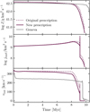 |
Fig. A.1. Evolution of total angular momentum (top), surface specific angular momentum (middle), and rotational velocity (bottom) for a 20 M⊙ Brott model with vi = 300 km s−1, which is ∼0.4 × vcrit. The dotted line indicates the original calculation, the solid line shows the value recalculated using the new angular momentum loss prescription. A 20 M⊙ Geneva model (Eggenberger et al. 2021) is shown in gray in the top and bottom panels, with initial rotation set to 0.4 × vcrit. |
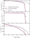 |
Fig. A.2. In the same style as Fig. A.1, but for a 40 M⊙ Brott model with vi = 350 km s−1, which is ∼0.4 × vcrit. The Geneva model (Eggenberger et al. 2021) shown in the top and bottom panels is 40 M⊙ with rotation set to 0.4 × vcrit. |
We use the 1D models of Eggenberger et al. (2021) as a comparison to our Brott models. These models are calculated with GENEC, the Geneva stellar evolutionary code. They have an initial metallicity of Z = 0.006, i.e., near a star in the Large Magellanic Cloud. These models take a different approach to angular momentum transport than Brott et al. (2011), accounting for hydrodynamical transport by the shear instability and meridional currents, and not considering internal magnetic fields. Therefore, they experience significant differential rotation during the MS, which is not seen in the Brott et al. (2011) models.
Fig. A.1 shows only small differences between the original and new data, as lower mass stars are less affected by stellar winds. The differences become more pronounced as the star approaches the end of its life, but are still very small. The Geneva model lives longer and does not show the sharp increase in angular momentum loss towards the end of its life. While spindown increases rapidly at ∼9.8 Myr, there is only a small increase in angular momentum loss rate at the same time.
In Fig. A.2 there is a steep decrease in angular momentum at ∼4.75 Myr, which corresponds to an increase in spindown and loss of surface specific angular momentum. The model reduces its rotational velocity at a more linear rate with our new angular momentum loss scheme, as opposed to the original approach, which shows two clear phases, before and after the ∼4.75 Myr mark. There is still a small increase in spindown with the new approach at that point, but since the model has already spun down so much it has minimal influence. Overall, the new scheme increases the amount of angular momentum lost, thereby reducing the impact of angular momentum transport and smoothing the rate of spindown. The Geneva model, however, shows marked differences. It lives for ∼6 Myr, rather than the ∼5 Myr seen in the Brott models, and loses much less angular momentum. While its initial rotation velocity is higher than that of the depicted Brott models, it spins down at a comparable rate.
Appendix B: Inflation
We have calculated a small model grid for massive MS stars with MESA, in order to investigate the effect of the convective efficiency on their envelope inflation and thus on their radius evolution (Sanyal et al. 2015). Notably, envelope inflation is confirmed by 3D-radiation-hydro calculations of the atmosphere of massive stars near their Eddington-limit (Jiang et al. 2015). We employ the standard mixing length theory for our experiment, and three different evolutionary sequences are computed per initial mass, using the canonical value for the mixing length parameter (αMLT = 1.5), as well as one significantly smaller (αMLT = 0.5) and one larger (αMLT = 5) value. Seven different initial masses in the range 20 M⊙ to 93 M⊙ have been considered.
As shown in Fig. B.1, the effect of the mixing length parameter on the location of the ZAMS is small (it becomes very significant for larger initial masses; see Fig. 20 in Köhler et al. (2015), and is blurred by the effect of envelope helium enrichment for the TAMS. However, the lines connecting the evolutionary mid-points, defined by models in which half of the hydrogen is burned in the core, show a clear dependence on αMLT above ∼40 M⊙. The models with the most efficient convection remain longer in the hotter part of the sHRD than the models with less efficient convection. To the extent that the stellar wind mass loss rate depends on stellar radius of effective temperature, angular momentum loss and spindown will be affected.
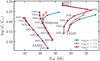 |
Fig. B.1. Spectroscopic Hertzsprung-Russell diagram showing the ZAMS line for different adopted values of the mixing length parameter αMLT for single-star evolutionary models at Z = 0.0092 with vi = 150 km s−1. On the left are the ZAMS lines for αMLT = 0.5 (teal), αMLT = 1.5 (orange, the standard value), and αMLT = 5.0 (pink). They overlap for all but the highest considered masses. The middle lines mark the midpoint of the MS, determined as the point where half of the initial hydrogen has been burned in the core. These midpoint lines are for the same 3 αMLT values as for the ZAMS lines. The lines on the right mark the TAMS lines, for the same 3 αMLT values. The αMLT = 0.5 line (teal) terminates at 43 M⊙ and the αMLT = 1.5 line (orange) terminates at 72 M⊙, due to the models failing to converge above this point. |
All Figures
|
Fig. 1. Schematic diagram of the specific internal angular momentum j of a model as a function of radius coordinate r, illustrating the angular momentum loss prescriptions corresponding to Eqs. (1) and (2). The width of the hatched area indicates the radius range that contains the material that is removed from the model within one timestep, where R2 corresponds to the stellar surface of the considered model, and R1 marks the layer that becomes the stellar surface after the next timestep. The prescription implemented in the Brott models removes the angular momentum represented by the hatched area. The new prescription removes the angular momentum in the hatched plus the shaded area. |
| In the text | |
|
Fig. 2. Top: Illustration of the Hōkū interpolation process. The left panel shows the initial masses and ZAMS velocities of the grid models in purple and turquoise, and the simulated star is shown in red. The right panel shows the evolutionary models in a spectroscopic HR diagram and the interpolated effective temperature and spectroscopic luminosity of the simulated star. The crosses mark where the effective temperature and spectroscopic luminosity are interpolated from the grid models. Bottom: Resulting evolutionary track of the 27 M⊙, |
| In the text | |
|
Fig. 3. Evolution of the rotational velocity from ZAMS to TAMS of Brott models according to the new predictions (derived as discussed in Appendix A). Each panel shows a different initial mass, and the colors indicate the effective temperature over the course of the MS. The x-axis shows the current core hydrogen mass fraction (Xcore) divided by the initial core hydrogen mass fraction (Xcore, i). |
| In the text | |
|
Fig. 4. 2D KDE of the entire observed sample in the sHRD (background). The solid lines show the evolutionary tracks of Brott models at 20 M⊙, 25 M⊙, 30 M⊙, 35 M⊙, 40 M⊙, 50 M⊙, 60 M⊙, 80 M⊙, and 100 M⊙ with an initial rotational velocity of 200 km s−1. The dotted lines divide the MS into quarters, determined by the fraction of the initial core hydrogen mass fraction that has been burned. The white line indicates log g = 3.7 dex. Only stars to the left of this line were used to create the initial velocity KDE discussed in Section 4.2. |
| In the text | |
|
Fig. 5. Distribution of the projected rotational velocity for the observed stars with log g > 3.7 dex, overplotted with one- and two-component Gaussian KDEs (solid and dashed lines, respectively). |
| In the text | |
|
Fig. 6. Distributions of the projected rotational velocity, v sin i for the observed stars (yellow lines) and for the synthetic population (gray histograms), where the v sin i is calculated using the rotational velocities directly from the models of Brott et al. (2011). The four columns show the different quarters of the MS, as denoted above, and the four rows show the different mass bins, as denoted to the right. The numbers in the legends indicate the number of observed or simulated stars in the respective histograms (see Sect. 4.1). The simulated distribution reaches beyond the y-axis boundary in two panels, where for the 100–60 M⊙ mass bin, the fourth quarter reaches to 0.13, and for the 60–40 M⊙ mass bin, the fourth quarter reaches to 0.069. |
| In the text | |
|
Fig. 7. As Fig. 6, but with v sin i values for the synthetic population calculated by applying our new angular momentum loss recipe to the models of Brott et al. (2011), as discussed in Appendix A. The simulated distribution reaches beyond the y-axis boundary in four panels. For the 60–100 M⊙ mass bin, the third quarter reaches to 0.08 and the fourth quarter reaches to 0.17. For the 40–60 M⊙ mass bin, the fourth quarter reaches to 0.12. For the 30–40 M⊙ mass bin the fourth quarter reaches to 0.05. |
| In the text | |
|
Fig. A.1. Evolution of total angular momentum (top), surface specific angular momentum (middle), and rotational velocity (bottom) for a 20 M⊙ Brott model with vi = 300 km s−1, which is ∼0.4 × vcrit. The dotted line indicates the original calculation, the solid line shows the value recalculated using the new angular momentum loss prescription. A 20 M⊙ Geneva model (Eggenberger et al. 2021) is shown in gray in the top and bottom panels, with initial rotation set to 0.4 × vcrit. |
| In the text | |
|
Fig. A.2. In the same style as Fig. A.1, but for a 40 M⊙ Brott model with vi = 350 km s−1, which is ∼0.4 × vcrit. The Geneva model (Eggenberger et al. 2021) shown in the top and bottom panels is 40 M⊙ with rotation set to 0.4 × vcrit. |
| In the text | |
|
Fig. B.1. Spectroscopic Hertzsprung-Russell diagram showing the ZAMS line for different adopted values of the mixing length parameter αMLT for single-star evolutionary models at Z = 0.0092 with vi = 150 km s−1. On the left are the ZAMS lines for αMLT = 0.5 (teal), αMLT = 1.5 (orange, the standard value), and αMLT = 5.0 (pink). They overlap for all but the highest considered masses. The middle lines mark the midpoint of the MS, determined as the point where half of the initial hydrogen has been burned in the core. These midpoint lines are for the same 3 αMLT values as for the ZAMS lines. The lines on the right mark the TAMS lines, for the same 3 αMLT values. The αMLT = 0.5 line (teal) terminates at 43 M⊙ and the αMLT = 1.5 line (orange) terminates at 72 M⊙, due to the models failing to converge above this point. |
| In the text | |
Current usage metrics show cumulative count of Article Views (full-text article views including HTML views, PDF and ePub downloads, according to the available data) and Abstracts Views on Vision4Press platform.
Data correspond to usage on the plateform after 2015. The current usage metrics is available 48-96 hours after online publication and is updated daily on week days.
Initial download of the metrics may take a while.