Predicting the length of magnetic cycles in late-type stars

R. Lorente; B. Montesinos

doi:10.1051/0004-6361/202554913

Home

All issues

Volume 702 (October 2025)

A&A, 702 (2025) A179

Full HTML

Open Access

Issue		A&A Volume 702, October 2025


Article Number		A179
Number of page(s)		15
Section		Stellar atmospheres
DOI		https://doi.org/10.1051/0004-6361/202554913
Published online		17 October 2025

A&A, 702, A179 (2025)

II. Solar and stellar butterfly diagrams: A forked dynamo model

R. Lorente¹^★ and B. Montesinos²

¹ European Space Astronomy Centre (ESAC) European Space Agency (ESA), Camino Bajo del Castillo s/n, 28692 Villanueva de la Cañada, Madrid, Spain
² Centro de Astrobiología (CAB), CSIC-INTA, ESAC Campus, Camino Bajo del Castillo s/n, 28692 Villanueva de la Cañada, Madrid, Spain

^★ Corresponding author.

Received: 31 March 2025
Accepted: 3 June 2025

Abstract

Aims. We present a one-dimensional dynamo model, along with its application to a sample of late-type stars with well-determined activity cycles.

Methods. In addition to reproducing the observed dependence of the cycle period, P_cyc, on the stellar rotation period, P_rot, for the stars in the sample, the model also reproduces the main properties of the solar butterfly diagram and generates possible magnetic diagrams for the other stars.

Results. The adopted interface dynamo model, which incorporates the essential magnetic generation processes, needs to be modified into a ‘forked dynamo’ at high latitudes to generate strong magnetic fields near the equator. This simple model offers an intuitive view of the dynamo mechanisms that might be operating in the stellar interiors.

Key words: stars: activity / stars: late-type / stars: magnetic field / stars: rotation / stars: solar-type / starspots

© The Authors 2025

Open Access article, published by EDP Sciences, under the terms of the Creative Commons Attribution License (https://creativecommons.org/licenses/by/4.0), which permits unrestricted use, distribution, and reproduction in any medium, provided the original work is properly cited.

This article is published in open access under the Subscribe to Open model. Subscribe to A&A to support open access publication.

1 Introduction

After the discovery of the Ca II H and K lines (396.85 and 393.37 nm, respectively) in the solar spectrum (Young 1872), attempts were made to observe similar features in other stars (Mitchell 1906; Hale & Adams 1906) in the proposed context of the ’solar-stellar connection’ (Hale 1905) (see also Thomas & Weiss 2008). The first detection of these chromospheric lines in a small sample of stars was reported by Eberhard & Schwarzschild (1913), suggesting the hypothesis of eruptive phenomena on stars similar to those observed on the Sun. This conjecture was confirmed over the years, starting with the compilation of Joy & Wilson (1949), where it was demonstrated that Ca II emission is not universal, but, rather, it is typical of late-type stars. Subsequently, Linsky (1970) and Linsky et al. (1979) showed that the stellar profiles in high-resolution spectra are similar to those observed in the solar surface, establishing a correspondence to the Sun’s activity and higlighting Ca II emission as a signature of stellar magnetic activity.

Although there were early attempts to detect variability in Ca II emission (Popper 1956), it was not until state-of-the-art technology enabled the monitoring campaign at Mount Wilson Observatory (see Wilson 1968 and Vaughan et al. 1978 for details of its history) that solid results were obtained. The first published data (Wilson 1978) included the detection of solarlike magnetic activity cycles in some 30 late-type stars (Saar & Brandenburg 1999). The correspondence between Ca II emission and magnetic flux, both in the Sun (Skumanich et al. 1975) and in solar-type stars (Schrijver et al. 1989), offers underlying evidence that variations in the Ca II emission reflect changes in the magnetic field on solar and stellar photospheres as well as in their interiors, where the magnetic field is generated.

Since the discovery of the magnetic nature of the solar activity (Hale 1908), dynamo action has been commonly accepted as the generating mechanism, instead of solar vortices (Hale 1908) or the remains of a fossil magnetic field (Hoyle 1949). Parker (1955a) developed the first model of a migratory dynamo in which the combination of non-uniform rotation and cyclonic convection provides a mechanism for generating a toroidal magnetic field from a poloidal magnetic field and vice versa. His model reproduces the basic features of the magnetic phenomenology observed on the solar surface: the equatorward migration of sunspots and the alternating polarity of their fields. The connection between the evolution of the magnetic field generated in the solar interior and the observed magnetic field at the surface is the rise to the photosphere of the interior toroidal magnetic field due to magnetic buoyancy (Parker 1955b).

Although Parker’s work is considered to be the basis for all the subsequent models, the problem is still under debate because no unique theory is presently able to reproduce all the phenomena observed in the Sun. The mechanism of poloidal field regeneration, the required magnetic field intensity, the variation of the intensity and duration of solar cycles, and the effects of the magnetic field on the plasma are some of the more difficult questions to address, both physically and mathematically, and have motivated a number of partial solar models. A very detailed discussion of the various models, as well as their successes and failings, can be found in the review by Charbonneau (2010).

The location and intensity of the magnetic field generated in the solar interior have been the main drivers of the evolution of dynamo theory. Magneto-hydrodynamics (MHD) simulations showed that the magnetic field in the solar interior should be organised in the form of thin flux tubes surrounded by free-field environment (Spruit 1981; Kraichnan 1976). Considerations of flux coherence (Moreno-Insertis et al. 1995; Schüssler 1983) and the observed latitudes of bipolar magnetic regions at the solar surface and their tilt angle (the so-called Joy’s law, Hale et al. 1919), further supplemented by their modelling (Caligari et al. 1995; Choudhuri & Gilman 1987), indicated that the field strength inside those flux tubes must be of the order of ~10⁵ G. Under such conditions, while also working to overcome both the field-storage problem (Moreno-Insertis 1983) and the quenching of turbulent motions, the so-called α-quenching (Vainshtein & Cattaneo 1992; Charbonneau & MacGregor 1996), dynamo models located in the whole convection zone (Yoshimura 1972), concentrated at its base (Parker 1975), or even in the overshoot region just beneath it (Schmitt 1993; Gilman 1992; Schüssler 1983), finally led to the so-called interface dynamo model presented by Parker (1993). In that model, the dynamo action is split between two different layers: a toroidal field generated by differential rotation in the overshoot layer and a poloidal field produced by the α effect in the lower convection zone. An account of the main features of the solar (and stellar) dynamo can be found in the review by Thomas & Weiss (2008).

In Lorente & Montesinos (2005), hereafter Paper I, we adopted such an interface dynamo. A simple local approximation of the model was developed, where an arbitrary point in the stellar interior was chosen to assess the global temporal behaviour of the generated magnetic field. The location of the integration point was irrelevant, since the results were dominated by the differential rotation, rather than by the stellar interior parameters. The main success of the model was its ability to reproduce the dependence of the period of the observed cycles, P_cyc(obs), on the stellar rotation period, P_rot, for 25 stars of the Mount Wilson sample with well-defined activity cycles, a relationship that will be revisited in Section 2. The model also generated magnetic fields of the required strength. Educated guesses and reasonable scalings were applied to the different ingredients of the model, with the aim of introducing the less possible number of free parameters.

Because of its limitations, a local dynamo cannot reproduce the temporal evolution of the latitudinal distribution of the solar surface magnetic field (the so-called solar butterfly diagram) or its analogues in the stellar sample. This shortcoming is the main motivation for developing the improved model presented here. It is still limited in scope, since it does not incorporate the dynamo equations in the whole stellar interior or in a radially expanded generation region; however, the new model has the advantage of accounting for both the depth at which the dynamo mechanism operates and its spatial boundaries. Also, the fact that the generation layer is likely to be very thin justifies the extension of the model only in the latitudinal dimension as a first approximation.

In addition, the model is applied to a sample of solar-type stars, attempting to reproduce some of their observed properties and infer other characteristics. It is noteworthy for obvious reasons, details on the position and the temporal and spatial evolution of starspots are scarce, the main advances having been done for highly spotted stars. Alekseev & Gershberg (1996) modelled the ‘spottedness’ of the flare star EV Lac, which seems to be dominated by an heterogeneous equatorial (latitude ~0°) band of spots. Petit et al. (2004), using Zeeman-Doppler imaging techniques, mapped polar spots on the surface of the K1 sub-giant of the HR 1099 close-binary system. Berdyugina, & Henry (2007) generated a butterfly diagram for the same star, which shows a mixture of pole and equatorward migration of different spot regions. Katsova et al. (2003) revealed that even highly spotted stars (very active, fast rotators) exhibit equator-ward migration of the stellar spots. The promising results of Katsova et al. (2010) are the most relevant to the present paper, carrying out the first attempt to derive butterfly diagrams for two stars, namely, HD 115404 and HD 149661, included in the sample analysed here, using the H-K Mount Wilson records. They found a trend of slower rotation at stellar maxima (e.g. possible poleward migration), but since both stars show double periodicities, it was difficult to reach a definitive conclusion.

In summary, the work presented in this paper presents a study of the generation and appearance of the magnetic field at the stellar surface, while incorporating the different ingredients of the dynamo and their effects on the field morphology, cycle period, and other surface observed properties. However, this is not an attempt by any means to stand as a global, self-consistent MHD model of the magnetic field. Instead, its aim is to use simple principles to reproduce the behaviour of two main features of the solar surface magnetic field, namely, its latitudinal distribution and its periodicity. The model does not attempt either to tackle the important issue of the origin of the grand minima, postulated to be caused in the solar case by a time-dependent torque exerted by the planets on a non-spherical tachocline (see e.g. Abreu et al. 2012; Albert et al. 2021).

The paper is organised as follows. In Sect. 2, we describe the sample of stars. In Sect. 3, we offer a description of the equations of the dynamo model. In Sect. 4, we give details on the calibration of the one-dimensional model. Section 5 deals with the differential rotation profiles and Sect. 6 describes the forked dynamo approach we have introduced. Sections 7 and 8 are devoted to discuss the results and summarise the conclusions of the work.

2 Sample of stars: P_cycle–P_rot relationship

As in Paper I, the sample of stars is essentially the same as the one considered by Brandenburg et al. (1998), which is a selection of those stars from Baliunas et al. (1995) showing a cycle detection with a low false-alarm probability FAP ≤ 10⁻⁵. In the context of the whole Mount Wilson campaign, Baliunas et al. (1995) described the temporal behaviour of stellar magnetism as an evolutionary gradation, from young high-activity stars with non-cyclic variations to old stars with lower rotation rates, smooth cycles, and occasional Maunder-minimum-like temporal states, based on the set of stars with clear cyclic behaviour (just ~30% of the whole sample). Katsova et al. (2003), using multi-colour photometric campaigns, unexpectedly discovered cycles in strongly spotted stars classified as ‘variable’ in Saar & Brandenburg (1999), showing that the detection of activity cycles depends on the observational proxies used.

Our selection is justified because the goal is to predict cyclic behaviours similar to that observed in the Sun. This natural limitation comes from the lack of knowledge about some essential ingredients of the dynamo mechanism, forcing the assumption of solar analogies by applying some scaling factors. Very active stars were excluded from the sample, since most of them are in close binary systems where tidal effects could distort a solarlike dynamo (Saar & Brandenburg 1999). Moreover, despite the fact that the periodograms give an uncertainty of only ±1 yr, the intrinsic variation of the length of solar magnetic cycles from ~9 to ~13 yr (from data recorded since 1750) is also seen in other stars of the sample (e.g. HD 100180, HD 201091, and HD 201092), which exhibit changing cycles (Oláh et al. 2009).

This variation in the length of the cycles is a complex phenomenon that a simple dynamo model cannot explain. Finally, as pointed out by Hall et al. (2007b), some of the stars might be entering a grand minimum phase, indicated by a transition between a cycling and a non-cycling state, during which the cycle duration could be distorted with respect to the normal cycle. This was the case for the Sun during the Maunder minimum, as discovered in ¹⁰Be records from Greenland ice cores (Beer et al. 1998; Beer 2000).

The basic parameters of the sample, spectral type, B-V, P_rot, and P_cyc(obs), were presented in Table 1 in Paper I, with the corresponding references. Here, they are reproduced in Table 1, with some updates. Cycle periods derived from periodogram analysis have been confirmed in independent works using wavelet-transform methods (Frick et al. 1997). Cycles were also detected in X-ray campaigns (see e.g. Favata et al. 2004). The sample could have been expanded by including the magnetic cycles derived photometrically by Oláh et al. (2009), but since their dataset is dominated by giants, sub-giants, and binary stars, we preferred to restrict our study to the original sample tested in Paper I. The sample has been enlarged with data for six stars (with two of them already in the original sample) from Messina & Guinan (2003). Table 2 shows the relevant properties for these objects.

For the sake of simplicity, stars other than the Sun have been classified as young (P_rot < 30 d; group 1 in Paper I) and old (P_rot > 30 d; groups 2 and 3 in Paper I). The main difference between young and old stars is that at P_rot shorter than ~30 d an onset of ’non-solar’ behaviour can be seen, characterised by double periodicities. This division is similar to the very preliminary one made by Noyes et al. (1984) between young and old stars as marked by the Vaughan-Preston gap (Vaughan & Preston 1980), which occurs at $\log R_{HK}^{'} ~ - 4.75$ $\log R_{{\rm{HK}}}^\prime \~ - 4.75$ (Brandenburg et al. 1998) and represents the boundary between a sort of chaotic behaviour (active stars), and solar-like temporal behaviour (old stars).

Baliunas et al. (1995) showed that stars close to the Vaughan-Preston gap tend to exhibit double periodicities. Moreover, according to Lockwood et al. (2007), $\log R_{HK}^{'} ~ - 4.7$ $\log R_{{\rm{HK}}}^\prime \~ - 4.7$ marks the boundary between spot-dominated (young) and faculae-dominated (old) behaviour. This classification differs slightly from the one by Saar & Brandenburg (1999), where stars with double periodicities are classified as active or inactive depending on the trend followed by its primary, P_cyc(obs), (log P_rot/P_cyc(obs) versus log Ro⁻¹ ). See et al. (2016) found a cut-off in the magnetic field topology at P_rot ≈ 12 d. According to our classification, HD 100180 and HD 190406 would belong to the young group, whereas the classifications mentioned above would classify them as inactive stars; however, their secondary period would put them in the active branch of Saar & Brandenburg (1999). As we show in this work, our classification is compatible with the same dynamo mechanism operating in both young and old stars, although there might be other kind of dynamos operating simultaneously in young stars that would produce a different periodicity (primary or secondary).

In line with Paper I, the relationship driving the efforts of the current dynamo model is the observed trend, $P_{cyc} (obs) \propto P_{rot}^{1.21 \pm 0.10}$ ${P_{{\rm{cyc}}}}\left( {{\rm{obs}}} \right) \propto P_{{\rm{rot}}}^{1.21 \pm 0.10}$ (presented again in Fig. 1). This trend spans both the inactive stars and the short period of active stars, excluding the Sun. We did indeed recover the simple relation obtained by Noyes et al. (1984), namely, $P_{cyc} (obs) \propto P_{rot}^{1.25 \pm 0.5}$ ${P_{{\rm{cyc}}}}\left( {{\rm{obs}}} \right) \propto P_{{\rm{rot}}}^{1.25 \pm 0.5}$ ; among other advantages, this relation allows us to avoid the introduction of theoretical parameters, such as the convective turnover time, τ_c, used in some correlations (Saar & Brandenburg 1999). Kleeorin et al. (1983) predicted different P_cyc versus P_rot trends depending on the rotation rate, which could be in some sense confirmed by the A (active) and I (inactive) branches observed by Brandenburg et al. (1998). The relationship shown in Fig. 1 corresponds mainly to the I branch in Brandenburg et al. (1998); the A branch (not clear in Paper I) has become visible here thanks to an enlargement of the original sample with the set of young solar analogues from Messina & Guinan (2003), with activity periods determined photometrically (see Table 2). These are shown as blue symbols in Fig. 1. Two of the stars in Messina & Guinan (2003) are common to our original sample: HD 1835 shows P_cyc(obs) = 9.1 yr (Paper I) and 6.7 yr (Messina & Guinan 2003), and HD 20630 shows P_cyc(obs) = 5.6 and 5.9 yr (same references). Both sets of values are plotted in Fig. 1. At a very short P_rot, both branches get mixed up. For consistency with Paper I, we did not include the new sub-sample of rapid rotators in the validation of our model. In this context, it is worth pointing out that HD 17051 (a F8 main-sequence star not included in our sample) is in complete agreement with the short period tail of our graphic, with P_rot ≃ 8 d and the shorter P_cyc detected thus far in single dwarf stars, P_cyc = 1.6 yr (Metcalfe et al. 2010; Sanz-Forcada et al. 2013).

The idea of the same dynamo mechanism operating in all stars in the sample underlies one of the main conclusions of Soon et al. (1993). Specifically, the shorter period of some of the young stars with double periodicities seem to belong to the same group as the periods of the older stars in the (P_cyc/P_rot)² versus age relationship, with (P_cyc/P_rot)² considered as the observable parametrisation of the dynamo number. In this context, a single dynamo model should be able to reproduce the trend of P_cyc(obs) versus P_rot seen in the ‘I’ branch of Saar & Brandenburg (1999), down to the ‘short’ tail, both for ‘active’ stars with a short primary period and ‘active’ stars with a short secondary period. In doing so, the active branch of Saar & Brandenburg (1999), namely, the longer P_cyc of the most rapid rotators, together with the solar Gleissberg period, would fall outside the scope of the present model. For the same reason, the very short activity periods of very active stars (P_rot < 3 d) that appear to occupy a new third branch with a different ω_cyc/Ω trend in Saar & Brandenburg (1999) would potentially be related to a different type of dynamo. The fact that our sample is so restricted makes this impossible to confirm; hence, we are not able to aptly reproduce the evolutionary trends of activity cycle with rotation period predicted by Kleeorin et al. (1983) solely based on this sample.

Table 1

Sample of stars.

Table 2

Stars from Messina & Guinan (2003), selected as an extension of the Paper I sample.

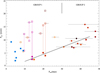Fig. 1

Relationship between P_cyc and P_rot for the stars in the original sample selected in Paper I and the young solar analogues from Messina & Guinan (2003) (blue squares), together with the fit to the original sample, log P_cyc(obs) = −0.95(±0.16) + 1.21(±0.11) log P_rot, which includes group 2 (except the Sun) and the shorter periods of the stars in group 1. The horizontal error bars cover the range [P_rot(max)–P_rot(min)] derived in Donahue et al. (1996).

3 The dynamo model

3.1 The underlying hypothesis and the scope of the model

The underlying hypothesis of the model is that the evolution of the latitudinal distribution of the toroidal magnetic field in the generation region buried in the solar interior is analogous to the time-latitude development of the spots and active regions on the surface of the Sun. This analogy is reasonable given to the high intensity of the generated magnetic field, which is immune to distortion due to turbulence as it rises to the surface (Moreno-Insertis 1986). Another essential condition to justify this hypothesis is that the effect of the Coriolis force, which could deflect the radial path of the flux tube, is negligible (Choudhuri & Gilman 1987; Caligari et al. 1995; Fan 2009). This is the case for stars similar to the Sun, in terms of their rotation rate and convective zone depth (Işık et al. 2011). As a further matter, theoretical stability studies in stellar interiors have shown that such stability depends on the latitude of the flux tube (Ferriz-Mas & Schüssler 1993, 1995). Thus, a given magnetic distribution down into the star would result in a different surface latitudinal magnetic distribution, apart from the effect of the meridional flows at different latitudes (Holzwarth et al. 2006).

Expanding the scope of the model to explore what can be said about stars other than the Sun, the observational stellar results mentioned in the introduction imply that well-established laws that apply to the Sun (e.g. the equatorward migration of sunspots, Hale’s polarity law, and Waldmeier’s relation between mean latitude of sunspots and the cycle intensity) might not apply to other stars. With this in mind, apart from trying to reproduce the period and intensity of the magnetic cycle done in the local approximation in Paper I, we set out to establish the validity of the new model for the solar case and to extend it to the stellar context according to the following three points.

The apt reproduction of Hale’s polarity law, so that the solar magnetic field is anti-symmetric with respect to the equator. Once this condition is met, predictions can be made for similar or different behaviours for the stars in our sample, which might then be verified in the future when new techniques are developed.
A recreation of the solar butterfly diagram. The aim is to find a parametrisation of the model such that the toroidal magnetic field generated in the solar interior migrates equatorward, while a weaker branch migrates polewards (Becker 1959; Stenflo 1988). As above, predictions would then be made for the stars in our sample.
Reproduction of Waldmeier’s law, according to which there is a positive correlation between the intensity of the solar cycle and the mean latitude of the sunspots (Waldmeier 1961; Lustig & Haupt 1986). Pulkkinen et al. (1999) showed a variation of ~3° in the mean latitude of sunspots for the last 12 cycles. This correlation cannot be reproduced as such, since the model is only able to generate purely cyclic behaviour without variations in duration or in intensity. However, it is possible to assess such a relationship in the stellar context, as if each individual solar cycle period would be considered to represent a slightly different star.

3.2 The dynamo equations

As in Paper I, the equations governing this model correspond to an αΩ kinematic dynamo action, in its mean field electrodynamics approach, which assumes that the velocity field is independent of a weak magnetic field. This is an assumption that must be critically assessed according to the latest helioseismology results, which show that there are changes in the differential rotation during the solar cycle (Suzuki 2014). We adopted the mean-field approximation (for more details, see Cowling 1981; Robinson & Durney 1982), where the turbulent component of the magnetic field is considered to be small compared to the mean field. The governing equations are $\begin{array}{l} \frac{\partial B_{ϕ}}{\partial t} = \nabla Ω \times (A_{ϕ} r \sin θ) + η_{T} (\nabla^{2} - \frac{1}{r^{2} \sin^{2} θ}) B_{ϕ} - \frac{u B_{ϕ}}{L}, \\ \frac{\partial A_{ϕ}}{\partial t} = α B_{ϕ} + η_{T} (\nabla^{2} - \frac{1}{r^{2} \sin^{2} θ}) A_{ϕ}, \end{array}$ $\matrix{ {{{\partial {B_\phi }} \over {\partial t}} = \nabla \Omega \times \left( {{A_\phi }r\,\sin \theta } \right) + {\eta _T}\left( {{\nabla ^2} - {1 \over {{r^2}{{\sin }^2}\theta }}} \right){B_\phi } - {{u{B_\phi }} \over L},} \hfill \cr {{{\partial {A_\phi }} \over {\partial t}} = \alpha {B_\phi } + {\eta _T}\left( {{\nabla ^2} - {1 \over {{r^2}{{\sin }^2}\theta }}} \right){A_\phi },} \hfill \cr }$ (1)

where B_ϕ is the mean toroidal magnetic field, A_ϕ is the vector potential of the mean poloidal field, and θ is the colatitude from the north pole. The scalar quantities α and η_T parametrise all the unknown mechanisms causing the generation and destruction of the magnetic field, although the physical interpretation of each of these terms has evolved, giving rise to different dynamo models (for a detailed review, see Charbonneau 2010). The term uB_ϕ/L represents the loss of magnetic field due to magnetic buoyancy (Parker 1979) and it is introduced as the prime non-linear mechanism that limits the dynamo action, following the discussion in Noyes et al. (1984). In the αΩ approach, α represents the generation term for the poloidal field, whereas the regeneration of the toroidal field takes place due to the action of the differential rotation ∇Ω.

Limiting the dynamo action to a thin layer, considering axisymmetry with respect to the rotation axis, and expanding the mathematical operators, the above equations (with sub-scripts dropped for simplicity) become $\begin{array}{l} \frac{\partial B}{\partial t} = \frac{\partial Ω}{\partial r} \frac{\partial}{\partial θ} (A \sin θ) + \frac{η}{r^{2} \sin θ} [\frac{\partial}{\partial θ} (\sin θ \frac{\partial B}{\partial θ}) - \frac{B}{\sin θ}] - \frac{u B}{L}, \\ \frac{\partial A}{\partial t} = α B + \frac{η}{r^{2} \sin θ} [\frac{\partial}{\partial θ} (\sin θ \frac{\partial A}{\partial θ}) - \frac{A}{\sin θ}], \end{array}$ $\matrix{ {{{\partial B} \over {\partial t}} = {{\partial \Omega } \over {\partial r}}{\partial \over {\partial \theta }}\left( {A\,\,\sin \,\,\theta } \right) + {\eta \over {{r^2}\sin \,\theta }}\left[ {{\partial \over {\partial \theta }}\left( {\sin \,\,\theta {{\partial B} \over {\partial \theta }}} \right) - {B \over {\sin \,\,\theta }}} \right] - {{uB} \over L},} \hfill \cr {{{\partial A} \over {\partial t}} = \alpha B + {\eta \over {{r^2}\sin \,\theta }}\left[ {{\partial \over {\partial \theta }}\left( {\sin \,\,\theta {{\partial A} \over {\partial \theta }}} \right) - {A \over {\sin \,\,\theta }}} \right],} \hfill \cr }$ (2)

which is a system of coupled non-linear differential equations with the time, t, and co-latitude, θ, as independent variables.

The latitudinal gradient of the rotation that appears in the expansion of the term ∇Ω × (A r sin θ), disappears in the one-dimensional approximation used here, but it plays an important role in two-dimensional dynamos. Yoshimura (1975) showed that the relative magnitudes of the radial and the latitudinal gradients determine the migration of the different branches of the magnetic field. In their study of interface dynamos, Charbonneau & MacGregor (1997) and Markiel & Thomas (1999) discussed the influence of the latitudinal gradient of Ω and demonstrated that it can actually dominate the dynamo in some cases.

Since the dawn of dynamo theory for stars, the convection zone has been considered the natural location of the mechanisms responsible for all the magnetic phenomenology observed at the stellar surfaces (Wilson 1966). However, subsequent studies have placed the dynamo mechanisms in preferred regions, from the whole convection zone (Yoshimura 1972) to the overshoot layer beneath it (Rüdiger & Brandenburg 1995) to prevent the generated magnetic field from rising prematurely due to its buoyancy (Parker 1975; Moreno-Insertis 1983; Ferriz-Mas & Schüssler 1995, 1993). In the case of the Sun, it is in the overshoot layer where most of the rotational shear is concentrated (Schou et al. 1998). This offers evidence that (at least partially) the dynamo is expected to act there.

Two-layer dynamos have been developed in parallel with single layer models, from the models of Deinzer & Stix (1971) or Stix (1973) to that of Moss et al. (2011). However, this does not rule out the possibility that a two-layer dynamo can reproduce surface magnetic wave migration, as seen for HR 1099. Boyer, & Levy (1992) attributed the multi-periodicities observed in the solar magnetic field to a combination of different dynamos operating in different layers with different turbulent magnetic diffusivities. Benevolenskaya (1998), Fletcher et al. (2010) and Broomhall et al. (2011) postulated a secondary dynamo located near the solar surface and fed by strong differential rotation, as an explanation of a ~2-yr acoustic signal sensitive to the magnetic field, detected in unresolved Sun-as-a-star Doppler velocity observations, similar to the ones found by analysing acoustic signals from CoRoT in other Sun-like stars (García et al. 2010). Furthermore, Böhm-Vitense (2007) suggested two different dynamos, originating in two different layers, as responsible for the A (active) and I (inactive) branches seen in the P_cyc versus P_rot and P_cyc/P_rot versus P_rot plots.

Parker (1993) introduced the concept of an interface dynamo in order to solve two problems: (i) the stability dilemma posed by dynamos operating in the convection zone proper is overcome by placing the generation of the toroidal field in the overshoot layer; and (ii) the problem related to the strong magnetic field in the overshoot region (Durney et al. 1990; Rüdiger & Brandenburg 1995) and its quenching of the α-effect (Schmitt & Schüssler 1989; Cattaneo et al. 1996) is solved by locating the generation of the poloidal field by the α effect in the bottom of the convection zone (for subsequent developments of the interface dynamo, see Charbonneau & MacGregor 1996, 1997; Markiel & Thomas 1999).

Here, we consider an interface dynamo acting into two separate, thin, contiguous layers: one at the bottom of the convection zone and the other in the overshoot layer below. The slight thickness of the generation layer in the convection zone was also supported by Markiel & Thomas (1999), who suggested that the toroidal field is rapidly removed from the convection zone by the effects of magnetic buoyancy and turbulent flux transport. This would indicate that the α effect operates only in the lower part of the convection zone, which is continuously fed by loops of the toroidal field that rise from the overshoot layer.

The so-called ‘tachocline’, named by Spiegel & Zahn (1992), is defined as the thin transition layer between the rigid rotation of the radiative solar interior and the differentially rotating convection zone. The thickness of the tachocline is derived theoretically in terms of the anisotropic turbulence (Spiegel & Zahn 1992), magnetic confinement (Gough & Mclntyre 1998), and the effect of a meridional circulation penetrating into the radiative core (Kitchatinov & Rüdiger 2006). Estimates of the thickness of the tachocline obtained from helioseismology vary from ~0.01 R_⊙ (Corbard et al. 1999) to ~0.09 R_⊙ (Kosovichev 1996) and it does not seem to change over the solar cycle (Corbard et al. 2001). Its location depends on latitude (Antia & Basu 2011): at low latitudes it lies mostly below the convection zone proper (Basu, & Antia 2001). Therefore, it would partially overlap with the overshoot layer, which has a predicted thickness of d = 0.02–0.04 R_⊙ according to non-local mixing length theories (Skaley & Stix 1991). As in Paper I, we assumed a spherical tachocline with constant thickness Δ_r ~ 0.5 H_bc, where H_bc is the pressure scale height at the bottom of the convection zone. Although the thickness of the tachocline is a crucial factor in our one-dimensional model, it is worth mentioning that some models predict a greater complexity of the spatial distribution of the magnetic field for thinner tachoclines (Moss et al. 1990; Rüdiger & Brandenburg 1995; Brandenburg 2005).

Since we are not resolving radial variations and, as in Paper I, we still need to parametrise the concept of an interface dynamo model by introducing ad hoc ‘transfer’ factors, T₁ and T₂, which represent, respectively, the fraction of poloidal field that diffuses into the overshoot region and the fraction of toroidal field that penetrates the convection zone; thus, we would have A_os = T₁ A_cz and B_cz = T₂ B_os. Similarly, the relationship between the magnetic diffusivities in both layers is f_η = η_os/η_cz (Parker 1993).

Scaling the variables A, t and u as in Paper I, we have $A = A' {| α / Ω_{r} |}^{1 / 2},$ $A = A\prime {\left| {\alpha /{\Omega _r}} \right|^{1/2}},$ (3) $t = t' {| α Ω_{r} |}^{- 1 / 2},$ $t = t\prime {\left| {\alpha {\Omega _r}} \right|^{ - 1/2}},$ (4) $u = u' {| H_{bc}^{2} α Ω_{r} |}^{1 / 2},$ $u = u\prime {\left| {H_{{\rm{bc}}}^2\alpha {\Omega _r}} \right|^{1/2}},$ (5)

and defining the dynamo number as $N_{d} = \frac{α Ω_{r} r_{cz}^{4}}{16 η_{cz}^{2}},$ ${N_{\rm{d}}} = {{\alpha \,{\Omega _r}\,r_{{\rm{cz}}}^4} \over {16\,\eta _{{\rm{cz}}}^2}},$ (6)

we obtain $\begin{array}{l} \frac{\partial B_{os}}{\partial t} = \frac{Ω_{r}}{| Ω_{r} |} \frac{\partial}{\partial θ} (T_{1} A_{cz} \sin θ) \\ + \frac{f_{η}}{4 {| N_{d} |}^{1 / 2} \sin θ} [\frac{\partial}{\partial θ} (\sin θ \frac{\partial B_{os}}{\partial θ}) - \frac{B_{os}}{\sin θ}] - u_{os} B_{os}, \\ \frac{\partial A_{cz}}{\partial t} = \frac{α}{| α |} T_{2} B_{os} + \frac{1}{4 {| N_{d} |}^{1 / 2} \sin θ} [\frac{\partial}{\partial θ} (\sin θ \frac{\partial A_{cz}}{\partial θ}) - \frac{A_{cz}}{\sin θ}], \end{array}$ $\matrix{ {{{\partial {B_{{\rm{os}}}}} \over {\partial t}} = {{{\Omega _{\rm{r}}}} \over {\left| {{\Omega _{\rm{r}}}} \right|}}{\partial \over {\partial \theta }}\left( {{T_1}{A_{{\rm{cz}}}}\sin \;\theta } \right)} \hfill \cr {\;\;\;\;\;\;\;\;\;\;\; + {{{f_\eta }} \over {4{{\left| {{N_{\rm{d}}}} \right|}^{1/2}}\sin \;\theta }}\left[ {{\partial \over {\partial \theta }}\left( {\sin \;\;\theta {{\partial {B_{{\rm{os}}}}} \over {\partial \theta }}} \right) - {{{B_{{\rm{os}}}}} \over {\sin \;\;\theta }}} \right] - {u_{{\rm{os}}}}{B_{{\rm{os}}}},} \hfill \cr {{{\partial {A_{{\rm{cz}}}}} \over {\partial t}} = {\alpha \over {\left| \alpha \right|}}{T_2}{B_{{\rm{os}}}} + {1 \over {4{{\left| {{N_{\rm{d}}}} \right|}^{1/2}}\sin \;\;\theta }}\left[ {{\partial \over {\partial \theta }}\left( {\sin \;\;\theta {{\partial {A_{{\rm{cz}}}}} \over {\partial \theta }}} \right) - {{{A_{{\rm{cz}}}}} \over {\sin \;\;\theta }}} \right],} \hfill \cr }$ (7)

where the tilde denoting non-dimensional variables has been omitted for simplicity. The first equation describes the production of the toroidal field in the overshoot region (sub-script ‘os’) and the second equation describes the evolution of the poloidal magnetic field in the convection zone (sub-script ‘cz’).

Equations (7) were solved using the forward time, centred space (FTCS) method (Press et al. 1992), ensuring that the time step is such that the various operators are stable for a given spatial step, Δθ,

Δt < 2|N_d|^1/2(Δθ)² and
Δt < 1/u,

which is normally dominated by the first condition, except for very large |N_d|. The initial conditions are chosen arbitrarily. After making sure that the initial transients disappear and that the final state is reached, it was determined that the steady-state solutions do not depend on the initial conditions. Finally, with respect to the boundary conditions, the one-dimensional approximation eliminates the need to define conditions at both the inner boundary with the stellar radiative interior and at the shallower surface, wherever it is defined. By integrating over both hemispheres, with constraints in the axis of symmetry, A(θ = 0) = B(θ = 0) = 0 and A(θ = π) = B(θ = π) = 0, we avoid the need to impose conditions at the equator. Therefore, the system will naturally evolve to a non-forced symmetric or antisymmetric solution.

4 Set-up and calibration of the one-dimensional model

The main ingredients in the dynamo model were presented in Paper I, using internal physical parameters derived from the FRANEC interior models (Chieffi & Straniero 1989). For completeness, we re-examine the different ingredients and their parametrisation here.

Starting with the simplest ones, we continued to adopt a classical approach for the diffusivity in the convection zone and, hence, for the diffusivity in the overshoot region, via the f_η parameter, η_cz ~ υ_czH, where υ_cz is the convective velocity and H is the pressure scale height. For the buoyancy velocity of the toroidal magnetic flux, we used the approach of Parker (1979), simplified by Markiel et al. (1994), expressed as $u_{os} = \frac{3 Q}{32} \frac{{| B_{os} |}^{2}}{4 π ρ_{cz} υ_{cz}},$ ${u_{{\rm{os}}}} = {{3Q} \over {32}}{{{{\left| {{B_{{\rm{os}}}}} \right|}^2}} \over {4\pi \,{\rho _{{\rm{cz}}}}\,{\upsilon _{{\rm{cz}}}}}},$ (8)

where Q ~ 1 in the convection zone and is much lower in the overshoot region. This follows the reasoning of Parker (1993), which posits that the magnetic flux tubes disturb the local distribution of the temperature and the heat transport of the surroundings, such that local phenomena cancel the buoyancy in the presence of a strong toroidal magnetic field.

In the local model of Paper I, the need to formulate explicitly the latitudinal dependency of both the α effect and the differential rotation was circumvented; however, these aspects are of crucial relevance in the current one-dimensional model, as shown below. Therefore, a justification of the choice of the latitudinal dependencies for both magnetic generation terms is needed.

Regarding the α effect, the classical Babcock-Leighton model (Babcock 1961; Leighton 1964), where the regeneration of the poloidal field from the toroidal component comes from the tilt of the bipolar magnetic regions at the surface and sub-sequent reconnection effects, was used by Jouve et al. (2010), but without success with respect to reproducing the observed P_cyc versus P_rot dependence seen in solar-type stars. In view of the drawbacks of that dynamo model (see also Charbonneau 2010 for a discussion), we adopted the simple parametrisation from Cowling (1981), α ∝ Ω Hcos θ, based on Parker’s idea of toroidal magnetic field lines twisted by the Coriolis force. As we have found in this work, this basic expression by itself creates stronger fields at the poles. Some attempts have been made to mitigate the strong polar branch induced by such an α effect (Charbonneau & MacGregor 1997; Markiel & Thomas 1999). For instance, in their detailed study of a general expression for α (i.e. α ~ cos θ sin^m θ), Moss et al. (2011) showed that a high value of m induces a sharper concentration of the magnetic field around the equator. We argue later in this paper that there is no need to modify the classical and intuitive α expression from Cowling (1981).

The explicit formulation of the radial differential rotation is much richer, thus, we devote Section 5 to exploring different options and dissect the various results. Here, we can analyse its scaling factors through all the stars in the sample. Various theoretical models have tried to predict the dependence of the internal rotation on the rotation rate or the Rossby number (Kitchatinov & Rüdiger 1995; Karak et al. 2015). The problems inherent in measuring the internal rotation profile from asteroseismology data in dwarf stars (Lund et al. 2014; Nielsen et al. 2017) makes it very difficult to confirm such findings observationally. Until now, only surface differential rotation has been measured. Various works confirm a weak dependence of the differential rotation on the rotation rate (Barnes et al. 2005; Reinhold et al. 2013; Das Chagas et al. 2016); whereas models predict a non-monotonic dependence (Kitchatinov & Olemskoy 2012; Küker & Rüdiger 2011). The dependence with spectral type has been confirmed by different observational and theoretical works (Barnes et al. 2005; Collier Cameron 2007; Kitchatinov & Olemskoy 2012; Reinhold et al. 2013; Balona, & Abedigamba 2016), although a stronger dependence for stars hotter than those in our sample was confirmed by observations (Reinhold et al. 2013) and models (Küker & Rüdiger 2011). Since our sample does not contain early F stars, for which the steepness of the relation is concentrated and has more in common with the sample studied by Donahue et al. (1996), we justify the use of their simple dependence with rotation rate. This approach was already used in Paper I, ΔΩ ∝ Ω^0.7, however, we must not neglect the fact that the measured ΔΩ could be distorted due to the bias by the contributing active latitudes. Messina & Guinan (2003) obtained similar laws for younger stellar samples, which is also supported by theoretical models (Hotta & Yokoyama 2011).

Another uncertainty is the sign of the surface differential rotation. Different trends of the rotation period along the activity cycle have been deduced from observations. Donahue & Baliunas (1994) described cases going from solar (rotational period increasing along the starspot cycle) to anti-solar, passing through alternate trends along the activity cycle – or even non-modulated or hybrid rotation patterns. It should be noted that non-solar behaviour could be due either to non-solar differential rotation or non-solar activity migration, among other effects, probably due to the fact that a poleward migration similar to the high-latitude solar branch could have dominated the rotational modulation depending on the stellar inclination (Messina & Guinan 2003). The compilation by Moss et al. (2011) describes more extreme cases deduced by Doppler imaging, such as HR 1099, which shows two branches with opposite migrations concentrated at mid and high latitudes, or the presence of standing waves as in AB Dor. We note that the authors did attempt to reproduce theoretically the non-solar behaviours without invoking anti-solar differential rotation patterns. Models from Gastine et al. (2014) have shown that the transition from solar (faster rotation at the equator) to anti-solar (slower rotation at the equator) differential rotation occurs at Ro ~ 1. Therefore anti-solar behaviour would mainly affect the warmer or slower stars in our sample. Anti-solar surface differential rotation has been observed for a few K giant stars, mainly in binary systems (Strassmeier et al. 2003; Kovári et al. 2007; Weber et al. 2005), although Reinhold & Arlt (2015) did not rule out antisolar behaviour among 50 Kepler G-type stars. For the purposes of this work, we ignored these findings, since they would open a new parameter space and nullify the validity of a single dynamo model for the whole sample.

Finally, we chose T₁ = T₂ = 0.1, so that 10% of magnetic field would be able to diffuse from one layer to the other. We also retained the value f_η = 10⁻² as in Paper I, as a trade-off between too small or too large η_os values to ensure that the diffusion is strong enough to enable the transport of magnetic field from one layer to the other (Charbonneau & MacGregor 1997), but weak enough to allow for the regeneration of the magnetic field through the α effect. Since our model is one-dimensional and does not take into account the radial diffusion of the magnetic field, the first effect would be overlooked without notice; whereas the second one would be evident by itself in the nature of the solutions. Parker (1993) showed that the ratio between the toroidal magnetic field strength in the convection zone and in the overshoot region depends on the ratio of the corresponding turbulent diffusivities, $B_{os} / B_{cz} \propto f_{η}^{- 1 / 2}$ ${B_{{\rm{os}}}}/{B_{{\rm{cz}}}} \propto f_\eta ^{ - 1/2}$ . This justifies our choice of η_os: assuming the generation of equipartition fields at the base of the convection zone, B_cz(eq) = 10⁴ Gauss (Charbonneau & MacGregor 1996), gives B_os ~ 10⁵ Gauss, which is suggested by theory and observations.

As explained in Paper I, the scaling factors of the different ingredients could not be determined by calibrating the model using solar values, since it has been shown that in many phenomena, the Sun is not as standard as to be considered a prototype. The solar twin 18 Sco (Porto de Mello & da Silva 1997) shows photometric and spectroscopic behaviour similar to the Sun, although there are still doubts about its validity as a true solar twin (see for example Hall et al. 2009). Despite the fact that it has a rotation period similar to the Sun, P_rot = 22.7 d (Petit et al. 2008), it shows a somewhat greater activity level and a much shorter activity cycle, namely, P_cyc = 7.1 ± 0.2 yr (Hall et al. 2007b). Overplotting those values in Fig. 1, 18 Sco seems to follow the general P_cyc versus P_rot trend much better than the Sun does, which emphasises the need to use an ’artificial’ calibrator, as we did in Paper I. Therefore, an object with B – V = 0.94, P_rot = 40.2 d, and P_rot = 10.3 yr was used to fix the remaining free parameters, which were gathered altogether in the dynamo number N_d. This serves not only to calibrate the model, but also to explore different dynamo regimes.

5 Differential rotation profiles driving the dynamo action

5.1 Constant differential rotation profiles

For comparison with the local model presented in Paper I, with the awareness that it is not valid for the solar interior, we explored the dynamo generated by a uniform differential rotation profile throughout the whole generation region, $Ω_{r} = Δ Ω / Δ_{r},$ ${\Omega _r} = \Delta \Omega /{\Delta _{\rm{r}}},$ (9)

where Δ_r is the thickness of the tachocline, and ΔΩ = Ω_max – Ω_min, namely, the change in the rotation rate across the generation region.

In line with the previous interface dynamo models, there should be a strong radial rotation gradient in the overshoot region beneath the convection zone. Nevertheless, considering the undeniable fact that it is not only the Sun, but all the stars in the sample that present surface differential rotation, the transition from the surface rotation profiles to the purely radial shear in the overshoot region should occur in a layer with both latitudinal and radial shear. This is shown in Fig. 2 for the Sun, where the convective zone acts as a transition between the surface and internal rotation profiles. From Markiel & Thomas (1999), we took the solar values for the surface, both equatorial and polar, as well as for the internal rotation, so that the radial gradient for the Sun is given by the difference between the internal and surface rotations. For the remaining stars in the sample, Ω_r follows the law in Donahue et al. (1996), as discussed in the previous section and developed in Paper I. This rotation profile (see similar models used by Wilson 1992) would be compatible with the interface dynamo theory only if the latitudinal gradient of the rotation is smaller than the radial gradient. In turn, this would produce such weak magnetic fields in the convection zone that they would lose their coherence under the influence of the turbulent motions.

In view of the more realistic solar rotation profile that will be used in the following section, it is worth pointing out that: i) the radial shear in the overshoot region does not depend on latitude, so it does not produce a preferred latitude for dynamo generation; and ii) the radial shear has the same sign at all latitudes, through the whole tachocline.

We applied the one-dimensional dynamo model, with all the ingredients described in the previous section, to a star similar to the Sun, assigning to it a negative and moderate dynamo number N_d ≃ −70, close to the critical value of N_d for which a self-excited dynamo is maintained. It is tuned to produce a cycle period similar to the solar one. Fig. 3 shows the resulting latitudinal migration of the toroidal magnetic field (above) and its associated magnetic wave (below). As expected for a negative dynamo number, the wave propagates towards the equator and reproduces the anti-symmetry of sunspot polarity with respect to the equator and the rapid rise and slow decline observed in the sunspot migration and in the chromospheric records of the Mount Wilson sample (Waldmeier 1961; Baliunas et al. 1995).

The resulting polarity of the magnetic field produced by such a differential rotation profile depends on N_d, so its choice should be constrained in order to reproduce the solar butterfly diagram, whose pattern could be similar to that of the remaining stars in the sample (or, otherwise, the opposite). Fig. 4 represents the relationship between P_cyc and N_d that is used in a subsequent step of the analysis and it meant to explore different polarities as a function of N_d. In the regime of N_d < 0, a gradual increase in N_d increases the number of magnetic belts with alternating symmetric or anti-symmetric behaviour: if |N_d| < 70, the dynamo shows a symmetric behaviour, as a monopole centred at the equator; for N_d ~ 70 the anti-symmetric behaviour switches on and each hemisphere is dominated by an opposite polarity; around |N_d| = 1000 symmetry takes over, with two polarities in each hemisphere, one of them centred at the equator. For N_d > 0, the transition to different topologies appears at different dynamo numbers. As stated above, the actual outbreak of symmetric topology of the generated magnetic fields in our sample cannot be predicted with our simplified dynamo model, which has been calibrated simply to reproduce the solar behaviour; however, it does show that different topologies are possible for faster stellar rotations. Finally, Fig. 4 reproduces the plots from Saar & Brandenburg (1999) where different regimes were shown, opening up the possibility of different polarities within the magnetic field when different dynamo regimes are considered.

Fig. 4 also shows that the relationship between the computed cycle period, P_cyc(comp), and the dynamo number, N_d, depends on the N_d range. In other words, this depends on the N_d assigned to the calibrator, going from P_cyc(comp) ∝ |N_d|^−0.80 for small N_d to P_cyc(comp) ∝ |N_d|^−0.59 for higher N_d. Taking into account the rotation law from Donahue et al. (1996), the above relation transits from $P_{cyc} (comp) \propto P_{rot}^{1.4}$ ${P_{{\rm{cyc}}}}\left( {{\rm{comp}}} \right) \propto P_{{\rm{rot}}}^{1.4}$ to $P_{cyc} (comp) \propto P_{rot}^{1.0}$ ${P_{{\rm{cyc}}}}\left( {{\rm{comp}}} \right) \propto P_{{\rm{rot}}}^{1.0}$ . The compatibility with the observed P_cyc versus P_rot relationship shown in Fig. 1 demands dynamo numbers 10³ < |N_d| < 10⁴, which would translate in a non-observed symmetric parity for the Sun. An option to shift towards asymmetric topologies would be to increase the dependence of the dynamo number with the rotation by introducing an ad hoc dependence of the width of the tachocline with the rotation of the form Δ_r ∝ Ω^δ with δ = −0.4, in accordance with Paper I, so that Ω_r ∝ Ω^1.1. Assuming this law and assigning N_d = −700 to the synthetic calibrator, we ran the model for the whole sample. Thus, we obtained P_cyc(comp) ∝ |N_d|^−0.63, and $P_{cyc} (comp) \propto P_{rot}^{1.22 \pm 0.01}$ ${P_{{\rm{cyc}}}}\left( {{\rm{comp}}} \right) \propto P_{{\rm{rot}}}^{1.22 \pm 0.01}$ , as shown in Fig. 5, in perfect agreement with observations.

It is not a surprise that the generated magnetic field is not as confined about the equator as it should be for the Sun, due to the simple law for the α effect that is strengthened at the poles (∝ cos θ) and not compensated by a latitudinal differential rotation. The strongest magnetic field is produced in the latitude range 20°–30°, whereas the mean latitude of sunspots is 10°–15°. The difference cannot be due to the journey of the flux tubes through the convective zone, which would induce a deflection towards the poles due to the Coriolis force. It is important to point out that there are observed asymmetries in the surface solar magnetic field (Temmer et al. 2006), showing a light coupling between hemispheres, contrary to what is assumed in simple dynamo models.

As already mentioned, our model is only able to predict cycles with constant period, intensity, and mean latitude, preventing us from reproducing Waldmeier’s law, according to which the mean latitude of sunspots depends on the intensity of the cycle. Nevertheless, the stellar context can help in this regard. Using our model, we found that there is a gentle diminishing trend of the latitudinal location of the average magnetic field as a function of the magnetic intensity, with an amplitude of ~3° in the intensity range of the sample. This is not enough to reproduce the solar trend observed by Pulkkinen et al. (1999). The possibility that such a phenomenon does not come directly from the dynamo generation, but is instead an effect of the Coriolis force during the journey through the convection zone has not been ruled out; alternatively, the range of latitudes with magnetic fields observed in the Sun could be the result of the instability process that releases the flux tubes from the solar interior, depending on their intensity and latitude, so that more intense cycles might produce more unstable flux tubes at high latitudes (Schussler et al. 1994). In both cases, there would be a decoupling between the latitudes where sunspots appear and those where the dynamo process itself operates at deeper layers.

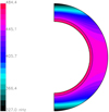Fig. 2

Rotation profiles with constant radial gradient in the overshoot region, taken for similarity with the local model developed in Paper I. The plotted region covers from the solar surface down to the bottom of the tachocline. The black contour indicates the bottom of the convection zone. Whereas the tachocline presents a purely radial gradient where the rotation varies from its equatorial value at the surface down to its constant value in the radiative interior, in the convection zone the rotation increases constantly from the poles to the equator and increases (decreases) from the surface towards the interior at high (low) latitudes. The figure represents the solar case, with Ω = 327.0 nHz at the poles, Ω = 457.7 nHz at the equator and Ω = 430.8 nHz in the interior, following the values of Markiel & Thomas (1999).

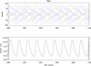Fig. 3

Top panel: latitudinal migration of the toroidal magnetic field obtained for the Sun. The plot shows the result of the integration of the one-dimensional dynamo model with a constant radial rotation profile in the generation region as main ingredient. Contours correspond to the maximum value of the B-field, and 4/5, 3/5, 2/5 and 1/5 of that value. Bottom panel: magnetic wave obtained as the averaged un-signed magnetic field at all latitudes.

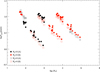Fig. 4

Variation of the cycle period computed with the one-dimensional model for various ranges of the dynamo number. Filled circles (open) squares are points with negative/positive N_d; red/black symbols represent magnetic fields symmetric (anti-symmetric) with respect to the equator.

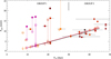Fig. 5

Relationship between P_cyc, both observed (see Fig. 1) and computed (diamonds), and P_rot for the stars of our sample. P_cyc has been computed with the one-dimensional dynamo model with a constant radial rotation profile and a assuming that the width of the tachocline varies with the rotation as explained in the text. Colours and symbols are as in Fig. 1. The fit plotted in black corresponds to the observed relationship presented in Fig. 1 and the fit in red to the one obtained with the computed cycles (the Sun excluded) with $P_{cyc} (comp) \propto P_{rot}^{1.22}$ ${P_{{\rm{cyc}}}}\left( {{\rm{comp}}} \right) \propto P_{{\rm{rot}}}^{1.22}$ .

5.2 Using a more realistic solar rotation profile

SOHO helioseismological data allows us to construct approximate patterns of the solar internal rotation. One example is those proposed by Schou et al. (1998), which show very strong radial differential rotation near the bottom of the convection zone and large uncertainties at high latitudes, depending on the depth (Gough 2013).

Markiel & Thomas (1999) applied a smooth analytic fit to the inversion terms of Schou et al. (1998), as follows, $Ω = {\begin{matrix} \begin{array}{l} Ω_{c} \\ Ω_{c} + \frac{(Ω_{s} (θ) - Ω_{c}) (r - 0.665 R_{⊙})}{0.05 R_{⊙}} \\ Ω_{s} (θ) \end{array} & \begin{array}{l} r < 0.665 R_{⊙}, \\ 0.665 R_{⊙} < r < 0.715 R_{⊙}, \\ 0.715 R_{⊙} < r, \end{array} \end{matrix}$ $\Omega = \{ \matrix{ {\matrix{ {{\Omega _{\rm{c}}}} \hfill \cr {{\Omega _{\rm{c}}} + {{\left( {{\Omega _{\rm{s}}}\left( \theta \right) - {\Omega _{\rm{c}}}} \right)\left( {r - 0.665{R_ \odot }} \right)} \over {0.05{R_ \odot }}}} \hfill \cr {{\Omega _{\rm{s}}}\left( \theta \right)} \hfill \cr } } & {\matrix{ {r < 0.665\,{R_ \odot },} \hfill \cr {0.665\,{R_ \odot } < r < 0.715\,{R_ \odot },} \hfill \cr {0.715\,{R_ \odot } < r,} \hfill \cr } } \cr }$ (10)

where r = 0.715 R_⊙ is the fractional radius at the base of the solar convection zone and r = 0.665 R_⊙ sets the bottom of the tachocline. Also, Ω_c and Ω_s(θ) are the rotation rates at the nucleus and at the solar surface, respectively, as follows, $\begin{array}{l} Ω_{c} = 430.8 nHz, \\ Ω_{s} (θ) = 457.7 - 57.9 \cos^{2} θ - 72.8 \cos^{4} θ nHz . \end{array}$ $\matrix{ {\,\,\,\,\,{\Omega _{\rm{c}}} = 430.8\,{\rm{nHz,}}} \hfill \cr {{\Omega _{\rm{s}}}\left( \theta \right) = 457.7 - 57.9{{\cos }^2}\theta - 72.8{{\cos }^4}\theta \,{\rm{nHz}}{\rm{.}}} \hfill \cr }$ (11)

The main features of such parametrisation, represented in Fig. 6 are: (i) purely radial profiles (∂Ω/∂r = 0) in the whole convection zone; (ii) a radial shear concentrated in the tachocline, constant in depth for all latitudes; and (iii) a change in the sign of the radial shear at θ = 55°, which is positive closer to the equator and negative closer to the poles.

Stellar differential rotation models show that the internal profiles depend strongly on the rotation rate (Hotta & Yokoyama 2011), making such a parametrisation for other stars invalid, especially for fast rotators for which the profiles should be more cylindrical. The colatitude at which surface and interior rotation rates match each other, and the extent and location of the shear layer could be different for different rotation rates. However, the restrictions imposed to our sample suggest that it is not unreasonable to assume stellar rotation profiles similar to that of the Sun and based on the features enumerated above.

Introducing these ingredients in the dynamo equations and normalising to the dynamo number at the equator, $N_{d} (eq) = \frac{α (eq) Ω_{r} (eq) r_{cz}^{4}}{16 η_{cz}^{2}},$ ${N_{\rm{d}}}\left( {{\rm{eq}}} \right) = {{\alpha \left( {{\rm{eq}}} \right){\Omega _r}\left( {{\rm{eq}}} \right)r_{{\rm{cz}}}^4} \over {16\eta _{{\rm{cz}}}^2}},$ (12)

we integrate the following system of equations $\begin{array}{l} \begin{array}{l} \frac{\partial B_{os}}{\partial t} = \frac{Ω_{r}}{| Ω_{r} (eq) |} \frac{\partial}{\partial θ} (T_{1} A_{cz} \sin θ) \\ + \frac{f_{η}}{4 {| N_{d} (eq) |}^{1 / 2} \sin θ} [\frac{\partial}{\partial θ} (\sin θ \frac{\partial B_{os}}{\partial θ}) - \frac{B_{os}}{\sin θ}] - u_{os} B_{os}, \end{array} \\ \begin{array}{l} \frac{\partial A_{cz}}{\partial t} = \frac{α}{| α (eq) |} T_{2} B_{os} \\ + \frac{1}{4 {| N_{d} (eq) |}^{1 / 2} \sin θ} [\frac{\partial}{\partial θ} (\sin θ \frac{\partial A_{cz}}{\partial θ}) - \frac{A_{cz}}{\sin θ}] . \end{array} \end{array}$ $\matrix{ \matrix{ {{\partial {B_{{\rm{os}}}}} \over {\partial t}} = {{{\Omega _{\rm{r}}}} \over {\left| {{\Omega _{\rm{r}}}\left( {{\rm{eq}}} \right)} \right|}}{\partial \over {\partial \theta }}\left( {{T_1}{A_{{\rm{cz}}}}\sin \;\theta } \right) \hfill \cr \;\;\;\;\;\;\;\;\;\;\; + {{{f_\eta }} \over {4{{\left| {{N_{\rm{d}}}\left( {{\rm{eq}}} \right)} \right|}^{1/2}}\sin \;\theta }}\left[ {{\partial \over {\partial \theta }}\left( {\sin \;\theta {{\partial {B_{{\rm{os}}}}} \over {\partial \theta }}} \right) - {{{B_{{\rm{os}}}}} \over {\sin \;\theta }}} \right] - {u_{{\rm{os}}}}{B_{{\rm{os}}}}, \hfill \cr} \hfill \cr \matrix{ {{\partial {A_{{\rm{cz}}}}} \over {\partial t}} = {\alpha \over {\left| {\alpha \left( {{\rm{eq}}} \right)} \right|}}{T_2}{B_{{\rm{os}}}} \hfill \cr \;\;\;\;\;\;\;\;\;\;\; + {1 \over {4{{\left| {{N_{\rm{d}}}\left( {{\rm{eq}}} \right)} \right|}^{1/2}}\sin \;\theta }}\left[ {{\partial \over {\partial \theta }}\left( {\sin \;\theta {{\partial {A_{{\rm{cz}}}}} \over {\partial \theta }}} \right) - {{{A_{{\rm{cz}}}}} \over {\sin \;\theta }}} \right]. \hfill \cr} \hfill \cr }$ (13)

Thus, we can obtain patterns of magnetic latitudinal evolution, such as those shown in Fig. 7. While for intermediate and negative N_d values, the dynamo generates steady magnetic fields (top panel of Fig. 7), for larger |N_d| a marked cyclic behaviour with alternating polarities occurs near the poles. The transition between the two behaviours happens at |N_d| ≈ 1000. Although the parameter space and the different regimes studied in Markiel & Thomas (1999) and in this work cannot be directly compared, the common features are the presence of steady fields and strong magnetism near the poles, where the α effect and the radial rotational gradient are stronger.

Instead of further confining the generation of the poloidal magnetic field to low latitudes by introducing less intuitive formulations for the α effect, a more natural approach would be to weaken the differential rotation near the poles. This is justified by the suggestion that depending on the inversion method adopted for the helioseismological data (Schou et al. 1998), the concentration of the radial gradient is smoothed out through the whole convection zone at high latitudes. Under such a hypothesis, we have introduced a new parametrisation of the solar rotation profile, as shown in Fig. 8. The key point of this new parametrisation is the presence of a radial shear in the convection zone, which calls into question the concept of the interface dynamo with two separate generation regions. It also requires the assumption that the fields generated there would be removed from the convection zone or destroyed in order to avoid their coherent rise to the surface – on timescales short enough so as not to disturb the rest of the system. As expected, such smoother profile do weaken the polar branch, as shown in Fig. 9, but such a dynamo is still dominated by the unrealistically strong quasi-steady magnetic field close to the equator.

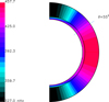Fig. 6

Differential rotation proflies in the solar interior, following Markiel & Thomas (1999) parametrisation of the original data from Schou et al. (1998). The angle θ = 55° sets the change of the sign of the radial gradient, being Ω_r > 0 nearer to the equator and Ω_r < 0 closer to the poles. r = 0.715 R_⊙ is the base of the solar convection zone and r = 0.665 R_⊙ sets the bottom of the tachocline.

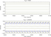Fig. 7

Latitudinal contours of the toroidal magnetic field at the bottom of the sub-adiabatic layer, B_os, obtained after applying the rotation profile from Markiel & Thomas (1999) to the one-dimensional interface dynamo model. Each panel corresponds to a different dynamo number, N_d = −500 at the top and N_d = −20000 at the bottom. The transition between the two behaviours happens at |N_d| ≈ 1000. Contours correspond to the same values of Β as in Fig. 3. The start time is selected in such a way that the initial numerical transients of the integration have disappeared and the behaviour of the magnetic field has already stabilised (this also applies to Figs. 9, 10, and 11).

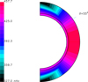Fig. 8

Differential rotation profiles in the solar interior, taken from Markiel & Thomas (1999) (see Fig. 6) but corrected at high latitudes in order to reproduce more closely the original data from Schou et al. (1998), according to which close to the poles the tachocline is not confined to a thin layer below the convection zone, but it extends towards the surface. This profile has been constructed so that at θ = 55° the tachocline extends over a fraction of the sub-adiabatic layer and expands towards the whole convection zone at θ ~ 30°.

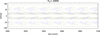Fig. 9

Latitudinal contours of the toroidal magnetic field at the bottom of the sub-adiabatic layer, B_os, obtained after applying to the one-dimensional interface dynamo model the rotation profile from Markiel & Thomas (1999) modified at high latitudes according to Fig. 8. Contours correspond to the same values of Β as in Fig. 3.

6 A forked dynamo

As shown in the previous section, a smooth radial rotation gradient that penetrates the convection zone leads to a mechanism that is no longer a pure interface dynamo. This is because at high latitudes, both the α effect and the differential rotation act together in the convection zone, whereas at low latitudes a pure interface dynamo model still occurs. We call this a ‘forked dynamo’, with a change in behaviour at colatitude θ₀. The equations to be integrated are different in the two latitude zones: $\begin{array}{l} \begin{array}{l} \frac{\partial B_{os}}{\partial t} = \frac{Ω_{r}}{| Ω_{r} (eq) |} \frac{\partial}{\partial θ} (T_{1} A_{cz} \sin θ) \\ + \frac{f_{η}}{4 {| N_{d} (eq) |}^{1 / 2} \sin θ} [\frac{\partial}{\partial θ} (\sin θ \frac{\partial B_{os}}{\partial θ}) - \frac{B_{os}}{\sin θ}] - u_{os} B_{os}, \end{array} \\ \begin{array}{l} \frac{\partial A_{cz}}{\partial t} = \frac{α}{| α (eq) |} T_{2} B_{os} \\ + \frac{1}{4 {| N_{d} (eq) |}^{1 / 2} \sin θ} [\frac{\partial}{\partial θ} (\sin θ \frac{\partial A_{cz}}{\partial θ}) - \frac{A_{cz}}{\sin θ}], \end{array} \end{array}$ $\matrix{ \matrix{ {{\partial {B_{{\rm{os}}}}} \over {\partial t}} = {{{\Omega _{\rm{r}}}} \over {\left| {{\Omega _{\rm{r}}}\left( {{\rm{eq}}} \right)} \right|}}{\partial \over {\partial \theta }}\left( {{T_1}{A_{{\rm{cz}}}}\sin \;\theta } \right) \hfill \cr \;\;\;\;\;\;\;\;\;\;\; + {{{f_\eta }} \over {4{{\left| {{N_{\rm{d}}}\left( {{\rm{eq}}} \right)} \right|}^{1/2}}\sin \;\theta }}\left[ {{\partial \over {\partial \theta }}\left( {\sin \;\theta {{\partial {B_{{\rm{os}}}}} \over {\partial \theta }}} \right) - {{{B_{{\rm{os}}}}} \over {\sin \;\theta }}} \right] - {u_{{\rm{os}}}}{B_{{\rm{os}}}}, \hfill \cr} \hfill \cr \matrix{ {{\partial {A_{{\rm{cz}}}}} \over {\partial t}} = {\alpha \over {\left| {\alpha \left( {{\rm{eq}}} \right)} \right|}}{T_2}{B_{{\rm{os}}}} \hfill \cr \;\;\;\;\;\;\;\;\;\;\; + {1 \over {4{{\left| {{N_{\rm{d}}}\left( {{\rm{eq}}} \right)} \right|}^{1/2}}\sin \;\theta }}\left[ {{\partial \over {\partial \theta }}\left( {\sin \;\theta {{\partial {A_{{\rm{cz}}}}} \over {\partial \theta }}} \right) - {{{A_{{\rm{cz}}}}} \over {\sin \;\theta }}} \right], \hfill \cr} \hfill \cr }$ (14)

for θ > θ₀. This identical to Equation (13) and then we have $\begin{array}{l} \begin{array}{l} \frac{\partial B_{os}}{\partial t} = \frac{Ω_{r}}{| Ω_{r} (eq) |} \frac{\partial}{\partial θ} (T_{1}^{'} A_{cz} \sin θ) \\ + \frac{f_{η}}{4 {| N_{d} (eq) |}^{1 / 2} \sin θ} [\frac{\partial}{\partial θ} (\sin θ \frac{\partial B_{os}}{\partial θ}) - \frac{B_{os}}{\sin θ}] - u_{os} B_{os}, \end{array} \\ \begin{array}{l} \frac{\partial B_{cz}}{\partial t} = \frac{Ω_{r}}{| Ω_{r} (eq) |} \frac{\partial}{\partial θ} (A_{cz} \sin θ) \\ + \frac{1}{4 {| N_{d} (eq) |}^{1 / 2} \sin θ} [\frac{\partial}{\partial θ} (\sin θ \frac{\partial B_{cz}}{\partial θ}) - \frac{B_{cz}}{\sin θ}] - u_{cz} B_{cz}, \end{array} \\ \begin{array}{l} \frac{\partial A_{cz}}{\partial t} = \frac{α}{| α (eq) |} B_{cz} \\ + \frac{1}{4 {| N_{d} (eq) |}^{1 / 2} \sin θ} [\frac{\partial}{\partial θ} (\sin θ \frac{\partial A_{cz}}{\partial θ}) - \frac{A_{cz}}{\sin θ}], \end{array} \end{array}$ $\matrix{ \matrix{ {{\partial {B_{{\rm{os}}}}} \over {\partial t}} = {{{\Omega _{\rm{r}}}} \over {\left| {{\Omega _{\rm{r}}}\left( {{\rm{eq}}} \right)} \right|}}{\partial \over {\partial \theta }}\left( {T_1^\prime {A_{{\rm{cz}}}}\sin \;\theta } \right) \hfill \cr \;\;\;\;\;\;\;\;\;\;\; + {{{f_\eta }} \over {4{{\left| {{N_{\rm{d}}}\left( {{\rm{eq}}} \right)} \right|}^{1/2}}\sin \;\theta }}\left[ {{\partial \over {\partial \theta }}\left( {\sin \;\theta {{\partial {B_{{\rm{os}}}}} \over {\partial \theta }}} \right) - {{{B_{{\rm{os}}}}} \over {\sin \;\theta }}} \right] - {u_{{\rm{os}}}}{B_{{\rm{os}}}}, \hfill \cr} \hfill \cr \matrix{ {{\partial {B_{{\rm{cz}}}}} \over {\partial t}} = {{{\Omega _{\rm{r}}}} \over {\left| {{\Omega _{\rm{r}}}\left( {{\rm{eq}}} \right)} \right|}}{\partial \over {\partial \theta }}\left( {{A_{{\rm{cz}}}}\sin \;\theta } \right) \hfill \cr \;\;\;\;\;\;\;\;\;\;\; + {1 \over {4{{\left| {{N_{\rm{d}}}\left( {{\rm{eq}}} \right)} \right|}^{1/2}}\sin \;\theta }}\left[ {{\partial \over {\partial \theta }}\left( {\sin \;\theta {{\partial {B_{{\rm{cz}}}}} \over {\partial \theta }}} \right) - {{{B_{{\rm{cz}}}}} \over {\sin \;\theta }}} \right] - {u_{{\rm{cz}}}}{B_{{\rm{cz}}}}, \hfill \cr} \hfill \cr \matrix{ {{\partial {A_{{\rm{cz}}}}} \over {\partial t}} = {\alpha \over {\left| {\alpha \left( {{\rm{eq}}} \right)} \right|}}{B_{{\rm{cz}}}} \hfill \cr \;\;\;\;\;\;\;\;\;\;\; + {1 \over {4{{\left| {{N_{\rm{d}}}\left( {{\rm{eq}}} \right)} \right|}^{1/2}}\sin \;\theta }}\left[ {{\partial \over {\partial \theta }}\left( {\sin \;\theta {{\partial {A_{{\rm{cz}}}}} \over {\partial \theta }}} \right) - {{{A_{{\rm{cz}}}}} \over {\sin \;\theta }}} \right], \hfill \cr} \hfill \cr }$ (15)

for θ < θ₀, where θ₀ is the colatitude at which the tachocline starts to penetrate the convection zone, which we have fixed to be θ₀ = 55°. The three equations to be integrated at high latitudes describe a classical self-contained dynamo in the convection zone where both generation mechanisms act simultaneously, allowing a very small fraction of poloidal field $(T_{1}^{'} = 0.01 T_{1})$ $\left( {T_1^\prime = 0.01\,{T_1}} \right)$ to be transferred to the overshoot region to feed the dynamo action there. It is also necessary to introduce a stronger magnetic buoyancy now present in the convection zone, taken ad hoc to be u_cz = 100 u_os.

By integrating the expressions in Equation (15), we obtain the magnetic profiles shown in Fig. 10, which still retain a very intense branch near the poles and an aperiodic general behaviour around the equator. The toroidal magnetic field generated in the convection zone is much more intense than the one generated in the sub-adiabatic region, where B_cz(max)~2 × 10⁸ Gauss in the former and B_os(max)~6 × 10⁵ Gauss in the latter. The dynamo in the convection zone is more efficient since it does not depend on the partial transport of magnetic field between layers. This dynamo would be classified as a ‘convection-zone mode’, as dubbed by Markiel & Thomas (1999). To avoid a convection-zone dominated dynamo, we introduce saturation mechanisms to inhibit convection-zone turbulence in the presence of strong magnetic fields, justified by the fact that the strength of the generated magnetic field is well above the equipartition level. A standard quenching of the α effect of the form (Robinson & Durney 1982) expressed as $α = c_{α} H_{cz} Ω \cos θ \exp (\frac{- γ B_{cz}^{2}}{4 π ρ υ_{cz}^{2}}),$ $\alpha = {c_\alpha }{H_{{\rm{cz}}}}\Omega \,\,\cos \,\,\theta \exp \left( {{{ - \gamma B_{{\rm{cz}}}^2} \over {4\pi \rho \upsilon _{{\rm{cz}}}^2}}} \right),$ (16)

which has the effect of reducing the generation of toroidal magnetic field in the convection zone (γ > 1 as free parameter) to ‘kill’ the undesired convection-zone modes; however, it has no effect on the intensity of the magnetic field generated in the sub-adiabatic layer, which would rise to the surface.

Integrating again the forked dynamo expressed in Equation (15), but including the α quenching, produces magnetic field profiles (shown in Fig. 11), which qualitatively reproduce the solar behaviour. A side effect of the α quenching at high latitudes is that it reduces the production of magnetic field and makes the polar branch disappear. Inspecting the field polarity regimes for different dynamo numbers (always with N_d < 0 to reproduce the magnetic migration of the Sun), we found that for |N_d| < 3000 the field is symmetric with respect to the equator, for 3000 < |N_d| < 35000 it is anti-symmetric, and for |N_d| > 35 000 the symmetry is triggered again, with both hemispheres having the same magnetic polarity. The latitudinal extension of the magnetic field does not change with the dynamo number.

Once the solar behaviour is reproduced for a certain range of N_d, we applied the ‘forked’ model to the rest of the sample. We kept all the free parameters for the whole sample untouched, except for the differential rotation. Since Ω_s(θ) and Ω_c are known only for the Sun, we scaled them in a simple way as a function of the star rotation, $\begin{array}{l} Ω_{s} (θ) = (P_{rot ⊙} / P_{rot}) \cdot Ω_{s ⊙} (θ), \\ Ω_{c} = (P_{rot ⊙} / P_{rot}) \cdot Ω_{c ⊙} . \end{array}$ $\matrix{ {{\Omega _{\rm{s}}}\left( \theta \right) = \left( {{P_{{\rm{rot}} \odot }}/{P_{{\rm{rot}}}}} \right)\, \cdot \,{\Omega _{{\rm{s}} \odot }}\left( \theta \right),} \hfill \cr {{\Omega _{\rm{c}}}\,\,\,\,\,\, = \left( {{P_{{\rm{rot}} \odot }}/{P_{{\rm{rot}}}}} \right)\, \cdot \,{\Omega _{{\rm{c}} \odot }}.} \hfill \cr }$ (17)

Fig. 12 shows the P_cyc(comp) computed with the forked model for all the stars in the sample, leading to a fit that takes the following form, $\log P_{cyc} (comp) = - 0.92 (\pm 0.02) + 1.21 (\pm 0.01) \log P_{rot},$ $\log \,{P_{{\rm{cyc}}}}\left( {{\rm{comp}}} \right) = - 0.92\left( { \pm 0.02} \right) + 1.21\left( { \pm 0.01} \right)\log {P_{{\rm{rot}}}},$ (18)

compatible with the observed trend. There was no need to scale the tachocline width with the rotation, as it was required for the local model. This comes naturally because Equation (17) already reflects a Ω_r ∝ Ω relationship.

Concerning the mean magnetic field generated in the over-shoot region, we could reasonably try to connect it to the field observed at the surface ${\bar{B}}_{s} \equiv f_{s} B_{s}$ ${\bar B_{\rm{s}}} \equiv {f_{\rm{s}}}{B_{\rm{s}}}$ , which is found to be correlated with the Rossby number, ${\bar{B}}_{s} \propto R o^{- 0.97 \pm 0.08}$ ${\bar B_{\rm{s}}} \propto R{o^{ - 0.97 \pm 0.08}}$ (Montesinos & Jordan 1993). Averaging over a whole hemisphere at the cycle maximum, $B_{os}^{max} = \bar{| B_{os}^{max} (0 ° \leq θ \leq 90 °) |}$ $B_{{\rm{os}}}^{{\rm{max}}} = \overline {\left| {B_{{\rm{os}}}^{{\rm{max}}}\left( {0^\circ \le \theta \le 90^\circ } \right)} \right|}$ , we find $B_{os}^{max} \propto R o^{- 0.78}$ $B_{{\rm{os}}}^{{\rm{max}}} \propto R{o^{ - 0.78}}$ . However, if we restrict the averaging to just the latitude range at which the classical interface dynamo operates, $B_{os}^{max} = \bar{| B_{os}^{max} (55 ° \leq θ \leq 90 °) |}$ $B_{{\rm{os}}}^{{\rm{max}}} = \overline {\left| {B_{{\rm{os}}}^{{\rm{max}}}\left( {55^\circ \le \theta \le 90^\circ } \right)} \right|}$ , we then find $B_{os}^{max} \propto R o^{- 0.90 \pm 0.03}$ $B_{{\rm{os}}}^{{\rm{max}}} \propto R{o^{ - 0.90 \pm 0.03}}$ . As shown in Fig. 13, this is compatible with a linear relationship between generated B_os and the observed fields. This would suggest that because of magnetohydrodynamic behaviour beyond the scope of this model, only the magnetic field generated by the pure interface dynamo at low latitudes reaches the surface and the magnetic field generated in the sub-adiabatic layer at high latitudes is not strong enough to emerge at the surface in the form of active regions.

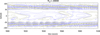Fig. 10

Latitudinal contours of the toroidal magnetic field generated at the sub-adiabatic layer, obtained as a result of the integration of the uni-dimensional forked dynamo model expressed in Equation (15), which do not include any quenching in the generation mechanisms. Contours correspond to the same values of Β as in Fig. 3.

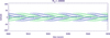Fig. 11

Latitudinal contours of the toroidal magnetic field of a forked dynamo including α quenching. Contours correspond to the same values of Β as in Fig. 3.

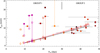Fig. 12

Similar to Fig. 5 but now with diamonds representing the cycles obtained from the integration of the ‘forked dynamo’. The red line corresponds to the fit P_rot – P_cyc(comp), in very good agreement with the observed P_rot – P_cyc(obs) relationship (black line).

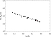Fig. 13

Magnetic field generated in the stellar interiors by a forked dynamo, as a function of the Rossby number, Ro. This magnetic field is the mean magnetic field generated up to the latitude where a pure interface dynamo model works. The fit corresponds to $B_{os}^{max} \propto R o^{- 0.90}$ $B_{{\rm{os}}}^{{\rm{max}}} \propto R{o^{ - 0.90}}$ .

7 Discussion

Simple assumptions about the governing parameters seem to be sufficient to build a reasonable dynamo model: an α effect with a simple latitudinal dependence to reflect the anti-symmetry of the Coriolis force about the equator, accompanied by a realistic parametrisation of the solar differential rotation that includes three different overlapping shear regions. There is a strong positive radial shear near the equator, a stronger negative radial shear near the poles (both of which determine the propagation direction of the dynamo waves according to the Parker-Yoshimura sign rule), and a latitudinal shear throughout the convective layer and the tachocline (Charbonneau 2010). Our one-dimensional approach is in fact equivalent to the numerical experiments carried out by Markiel & Thomas (1999). By suppressing the latitudinal gradient of the rotation, these authors were able to produce cyclic dynamos with a large diffusivity contrast between the generation layers (f_η = 10⁻²). In this vein, the new parametrisation of the solar rotation profiles presented in Fig. 8 appeases the latitudinal gradient in the overshoot layer, justifying its stealing of the limelight in the dynamo process. Only a fully two-dimensional model would be able to confirm that the radial gradient is indeed dominating the dynamo action.

As the natural transition from the local model in Paper I, the one-dimensional model presented in this work, with an unrealistic constant radial differential rotation, results in dynamo waves that propagate towards the equator and anti-symmetric with respect to the equator. They are both compatible with solar butterfly diagrams, but concentrated at higher latitudes than in the solar case, mainly due to the latitudinal distribution of the α effect (see Fig. 3).

Perhaps the biggest unknown of the dynamo model is the pattern of internal differential rotation. Seismology data taken from the space missions Kepler (Gilliland et al. 2010) and CoRoT (Baglin et al. 2006) have allowed us to infer, from the rotational splittings of mode frequencies, the internal rotation profiles of stars other than the Sun from massive stars (Pápics et al. 2014) and red giants (Beck et al. 2012; Deheuvels et al. 2012) to Sunlike stars (Ouazzani & Goupil 2012; Nielsen et al. 2014). Even in the solar case, there are still open questions about its differential rotation. Suzuki (2014) shows long-term variations of the solar surface differential rotation, from yearly to cycle-to-cycle trends, that would explain the intrinsic variation of the solar cycle and by analogy, the scatter in the P_cyc versus P_rot for the stars in the sample. Moreover there seems to be a de-coupling of the differential rotation between north and south solar hemispheres (Suzuki 2014; Li et al. 2013) that might explain Waldmeier’s law. Finally, the Maunder-minimum behaviour that has been reproduced with chaotic dynamo models (Beer et al. 1998; Usoskin et al. 2009), where cyclic behaviour persists but with lower intensity, could be understood in the much simpler framework of a variable differential rotation that can lead the star into different dynamo regimes – or even through more provocative hypothesis such as that mentioned in the introduction to the present paper (Abreu et al. 2012; Albert et al. 2021).

A realistic differential rotation profile, such as the smooth parametrisation of Schou et al. (1998) data in Markiel & Thomas (1999), which shows a very strong radial differential rotation near the bottom of the convection zone, results in steady magnetic waves and strong magnetism near the poles, where the α effect and the radial differential rotation are concentrated (see Fig. 7). Smoothing the radial shear at high latitudes, justified depending on the inversion method used in Schou et al. (1998), results in a dynamo still dominated by the unrealistically strong quasi-steady magnetic field close to the equator (as seen in Fig. 9).

As introduced in Section 6, a smooth radial rotation gradient in the convection zone leads to what we call a ‘forked dynamo’, a pure interface dynamo at low latitudes and a hybrid dynamo at high latitudes. Here, the convection zone harbours both generation mechanisms, differential rotation and α effect, together with a sub-adiabatic layer where only differential rotation operates. Fig. 10 shows the magnetic waves obtained with this new model, with very intense branch near the poles and a non-periodic pattern around the equator. The fact that this dynamo is more efficient in the convection zone than in the overshoot region would classify the model as ‘convection-zone dominated dynamo’; thus, we introduced saturation mechanisms to inhibit convection-zone turbulence in the presence of strong magnetic fields. This results finally in a magnetic wave that reproduces the main features of the solar butterfly diagram: restraint at low latitudes, equatorward migration, and alternating polarities between hemispheres (as shown in Fig. 11).

The simple parametrisation of the connection between the two generation regions that we use here should of course be overtaken by more complete MHD models. Our assumption of a similarity between the time-latitude diagrams at the magnetic generation region and the stellar surface butterfly diagrams is more in line with the global models of Işık et al. (2011), which combine the generation, instability, and transport of the magnetic flux. Accepting this assumption, a more complete picture should include the mechanism that concentrates the diffuse magnetic field produced in the solar interior into toroidal flux tubes, which is another missing ingredient needed to associate the magnetic field generated in the stellar interior with observed active regions.

Based on the local dynamo model in Paper I, it is appropriate to mention the role of our Sun among the stars in the sample. Although the Sun appears to have an activity level normal for its rotation period, age, and Ro (Mamajek & Hillenbrand 2008; Vidotto et al. 2014), the study by Barnes et al. (2005) showed that the differential rotation of the Sun is far weaker than what would be expected for its spectral type; however, it is still in good agreement with its rotation rate, which seems to be the governing parameter for magnetic cycles. Some authors tend to classify the Sun in an intermediate branch between inactive and active stars (e.g. do Nascimento et al. 2015).

Our dynamo model was forced to yield a purely harmonic and anti-symmetric behaviour of the magnetic field for the Sun (as seen in Fig. 11) as well as for the rest of the stars in the sample. Nevertheless, non-cyclical behaviour is found in other regimes (i.e. different differential rotation patterns or quenching phenomena), as seen in Figs. 7, 9, and 10. Such cases could potentially reproduce the non-cyclic behaviour seen in some stars in the Mount Wilson sample (Baliunas et al. 2006). The models developed by Kleeorin et al. (2023) showed that low-mass main sequences stars faster than the Sun can be dominated by mean-field α²Ω dynamos, resulting in chaotic behaviour in the magnetic activity.

The intensity of the magnetic field in the solar interior predicted by the model fits the upper limit of 0.3–1 MGauss derived from helioseismic frequency splittings (Gunther et al. 2015). The number of polar faculae, which, in turn, are correlated with the polar magnetic field measured with the Wilcox Solar Observatory (Sheeley 2008), are seen to lag behind the toroidal field associated with sunspots by π/2 (Sheeley 1991, 2008). Although this is usually interpreted in the framework of a flux-transport Babcock-Leighton dynamo (DeRosa et al. 2012), where the poloidal field is the result of the residual flux of decaying active regions that are advected polewards by meridional circulation, Charbonneau & MacGregor (1997) explained such a phase lag by comparing the toroidal field generated deep in the convection zone with the radial component of the poloidal field at the surface, both generated by an interface dynamo.

With our one-dimensional interface dynamo, we are only able to obtain the poloidal field in the generation region in the solar and stellar interiors. To argue that this poloidal field is related to the poloidal field observed at the solar surface is speculative and has nothing to do with the hypothesis of the sunspots being the non-distorted (from a macroscopic point of view) appearance at the surface of the flux tubes generated by the dynamo in the solar interior; in other words, the model predicts the distribution of fields in the stellar interior and we assume that what we see on the photosphere reflects that distribution. Even though the poloidal field obtained is nothing else than the seed that feeds the production of the toroidal field, it could be also seen as the average poloidal field produced in the convection zone and, in some sense, it could be related to the observed surface poloidal field. Fig. 14 shows when the toroidal field is positive and maximum (solid lines), namely, the maximum of the magnetic cycle with a certain polarity. This is also when the azimuthal potential vector is maximum with the same polarity, which must represent the maximum radial field, since B_r ∝ ∂A/∂θ in our one-dimensional approximation. As we can see in the plot, the toroidal field maxima lag by π/2 the radial field, invalidating the hypothesis of a direct link between the poloidal field generated in the solar interior and the one seen at the surface.

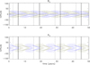Fig. 14

Latitudinal contours of the toroidal magnetic field obtained with a forked dynamo including α quenching. Top panel: toroidal field in the overshoot layer. Bottom panel: Azimuthal potential vector at the base of the convection zone. Solid lines represent the times when the positive toroidal field reaches its maximum and dashed lines show where the negative poloidal field is maximum. Contours correspond to the same values of Β as in Fig. 3.

8 Final remarks

As in the case of the local interface dynamo model presented in Paper I, the one-dimensional model presented in the present work, despite its simplicity, has proven successful in reproducing the P_cyc versus P_rot trend of the stars, demonstrating a clear cyclic behaviour in the Mount Wilson campaign, while also mimicking the pattern of the observed solar butterfly diagram down in the overshoot region beneath the convection zone. Potential butterfly diagrams have also been computed for stars other than the Sun. Substantial future efforts are needed to build a simple model that would integrate patterns that are not addressed in this work, such as double periodicities and the grand minima.

Acknowledgements

The authors are grateful to the referee for his/her review of the paper, and to Prof. John H. Thomas, for his many useful comments to the original manuscript. BM acknowledges the funding by grant PID2021-127289-NB-I00 from MCIN/AEI/10.13039/501100011033/ and FEDER.

References

Abreu, J. A., Beer, J. Ferriz-Mas, A., et al. 2012, A&A, 548, A88 [NASA ADS] [CrossRef] [EDP Sciences] [Google Scholar]
Albert, C., Ferriz-Mas, A., Gaia, F., & Ulzega, S. 2021, ApJ, 916, L9 [Google Scholar]
Alekseev, I. Y., & Gershberg, R. E. 1996, Cool Stars Stellar Syst. Sun, 109, 583 [Google Scholar]
Antia, H. M., & Basu, S. 2011, ApJ, 735, L45 [Google Scholar]
Babcock, H. W. 1961, ApJ, 133, 572 [Google Scholar]
Baglin, A., Auvergne, M., Barge, P., et al. 2006, The Corot Mission Pre-launch Status – Stellar Seismology and Planet Finding, 33 [Google Scholar]
Baliunas, S., & Soon, W. 1995, ApJ, 450, 896 [Google Scholar]
Baliunas, S. L., Donahue, R. A., Soon, W. H., et al. 1995, ApJ, 438, 269 [Google Scholar]
Baliunas, S. L., Nesme-Ribes, E., Sokoloff, D., et al. 1996, ApJ, 460, 848 [Google Scholar]
Baliunas, S., Frick, P., Moss, D., et al. 2006, MNRAS, 365, 181 [Google Scholar]
Balona, L. A., & Abedigamba, O. P. 2016, MNRAS, 461, 497 [NASA ADS] [CrossRef] [Google Scholar]
Barnes, J. R., Collier Cameron, A., Donati, J.-F., et al. 2005, 13th Cambridge Workshop on Cool Stars, Stellar Systems and the Sun, 560, 95 [Google Scholar]
Basu, S., & Antia, H. M. 2001, MNRAS, 324, 498 [Google Scholar]
Beck, P. G., Montalban, J., Kallinger, T., et al. 2012, Nature, 481, 55 [Google Scholar]
Becker, U. 1959, ZAp, 48, 88 [Google Scholar]
Beer, J. 2000, Space Sci. Rev., 94, 53 [Google Scholar]
Beer, J., Tobias, S., & Weiss, N. 1998, Sol. Phys., 181, 237 [Google Scholar]
Belvedere, G., Paterno, L., & Stix, M. 1980, A&A, 88, 240 [Google Scholar]
Benevolenskaya, E. E. 1998, ApJ, 509, L49 [Google Scholar]
Berdyugina, S. V., & Henry, G. W. 2007, ApJ, 659, L157 [Google Scholar]
Böhm-Vitense, E. 2007, ApJ, 657, 486 [CrossRef] [Google Scholar]
Boyer, D. W., & Levy, E. H. 1992, ApJ, 396, 340 [Google Scholar]
Brandenburg, A. 2005, ApJ, 625, 539 [NASA ADS] [CrossRef] [Google Scholar]
Brandenburg, A., Saar, S. H., & Turpin, C. R. 1998, ApJ, 498, L51 [NASA ADS] [CrossRef] [Google Scholar]
Broomhall, A.-M., Fletcher, S. T., Salabert, D., et al. 2011, Gong-SoHO 24: A New Era of Seismology of the Sun and Solar-like Stars, 271, 012025 [Google Scholar]
Caligari, P., Moreno-Insertis, F., & Schussler, M. 1995, ApJ, 441, 886 [Google Scholar]
Caligari, P., Schussler, M., Stix, M., et al. 1994, Cool Stars Stellar Syst. Sun, 64, 387 [Google Scholar]
Callebaut, D. K., & Makarov, V. I. 1992, Sol. Phys., 141, 381 [Google Scholar]
Cattaneo, F., Hughes, D. W., & Kim, E.-J. 1996, Phys. Rev. Lett., 76, 2057 [Google Scholar]
Charbonneau, P. 2010, Liv. Rev. Sol. Phys., 7, 3 [Google Scholar]
Charbonneau, P., & MacGregor, K. B. 1996, ApJ, 473, L59 [Google Scholar]
Charbonneau, P., & MacGregor, K. B. 1997, ApJ, 486, 502 [NASA ADS] [CrossRef] [Google Scholar]
Chieffi, A., & Straniero, O. 1989, ApJS, 71, 47 [NASA ADS] [CrossRef] [Google Scholar]
Choudhuri, A. R. 1990, ApJ, 355, 733 [Google Scholar]
Choudhuri, A. R., & Gilman, P. A. 1987, ApJ, 316, 788 [NASA ADS] [CrossRef] [Google Scholar]
Collier Cameron, A. 2007, Astron. Nachr., 328, 1030 [CrossRef] [Google Scholar]
Corbard, T., Blanc-Féraud, L., Berthomieu, G., et al. 1999, A&A, 344, 696 [Google Scholar]
Corbard, T., Jiménez-Reyes, S. J., Tomczyk, S., et al. 2001, SOHO 10/GONG 2000 Workshop: Helio- and Asteroseismology at the Dawn of the Millennium, 464, 265 [Google Scholar]
Cowling, T. G. 1953, The Sun, 532 [Google Scholar]
Cowling, T. G. 1981, ARA&A, 19, 115 [Google Scholar]
Das Chagas, M. L., Bravo, J. P., Costa, A. D., et al. 2016, MNRAS, 463, 1624 [Google Scholar]
Deheuvels, S., García, R. A., Chaplin, W. J., et al. 2012, ApJ, 756, 19 [Google Scholar]
Deinzer, W., & Stix, M. 1971, A&A, 12, 111 [Google Scholar]
Deluca, E. E., & Gilman, P. A. 1986, Geophys. Astrophys. Fluid Dyn., 37, 85 [Google Scholar]
DeRosa, M. L., Brun, A. S., & Hoeksema, J. T. 2012, ApJ, 757, 96 [NASA ADS] [CrossRef] [Google Scholar]
do Nascimento, J.-D., Saar, S. H., & Anthony, F. 2015, 18th Cambridge Workshop on Cool Stars, Stellar Systems, and the Sun, 18, 59 [Google Scholar]
Donahue, R. A., & Baliunas, S. L. 1994, Cool Stars Stellar Syst. Sun, 64, 396 [Google Scholar]
Donahue, R. A., Saar, S. H., & Baliunas, S. L. 1996, ApJ, 466, 384 [Google Scholar]
Durney, B. R., De Young, D. S., & Passot, T. P. 1990, ApJ, 362, 709 [Google Scholar]
Eberhard, G., & Schwarzschild, K. 1913, ApJ, 38, 292 [Google Scholar]
Fan, Y. 2009, Liv. Rev. Sol. Phys., 6, 4 [Google Scholar]
Favata, F., Micela, G., Baliunas, S. L., et al. 2004, A&A, 418, L13 [NASA ADS] [CrossRef] [EDP Sciences] [Google Scholar]
Ferriz-Mas, A., & Schüssler, M. 1993, Geophys. Astrophys. Fluid Dyn., 72, 209 [NASA ADS] [CrossRef] [Google Scholar]
Ferriz-Mas, A., & Schüssler, M. 1995, Geophys. Astrophys. Fluid Dyn., 81, 233 [Google Scholar]
Fletcher, S. T., Broomhall, A.-M., Salabert, D., et al. 2010, ApJ, 718, L19 [NASA ADS] [CrossRef] [Google Scholar]
Forgács-Dajka, E., Major, B., & Borkovits, T. 2004, A&A, 424, 311 [NASA ADS] [CrossRef] [EDP Sciences] [Google Scholar]
Frick, P., Baliunas, S. L., Galyagin, D., et al. 1997, ApJ, 483, 426 [Google Scholar]
García, R. A., Mathur, S., Salabert, D., et al. 2010, Science, 329, 1032 [Google Scholar]
Gastine, T., Yadav, R. K., Morin, J., et al. 2014, MNRAS, 438, L76 [CrossRef] [Google Scholar]
Gilliland, R. L., Brown, T. M., Christensen-Dalsgaard, J., et al. 2010, PASP, 122, 131 [Google Scholar]
Gilman, P. A. 1969, Sol. Phys., 8, 316 [Google Scholar]
Gilman, P. A. 1992, The Solar Cycle, 27, 241 [Google Scholar]
Glatzmaier, G. A. 1985, Geophys. Astrophys. Fluid Dyn., 31, 137 [Google Scholar]
Gough, D. 2013, Sol. Phys., 287, 9 [Google Scholar]
Gough, D. O., & McIntyre, M. E. 1998, Nature, 394, 755 [Google Scholar]
Gunther, H. M., Poppenhaeger, K., Testa, P., et al. 2015, 18th Cambridge Workshop on Cool Stars, Stellar Systems, and the Sun, 18, 25 [Google Scholar]
Hale, G. E. 1905, ApJ, 21, 124 [Google Scholar]
Hale, G. E. 1908, ApJ, 28, 315 [Google Scholar]
Hale, G. E., & Adams, W. S. 1906, ApJ, 23, 400 [Google Scholar]
Hale, G. E., Ellerman, F., Nicholson, S. B., et al. 1919, ApJ, 49, 153 [Google Scholar]
Hall, J. C., Henry, G. W., & Lockwood, G. W. 2007a, AJ, 133, 2206 [Google Scholar]
Hall, J. C., Lockwood, G. W., & Skiff, B. A. 2007b, AJ, 133, 862 [Google Scholar]
Hall, J. C., Henry, G. W., Lockwood, G. W., et al. 2009, AJ, 138, 312 [NASA ADS] [CrossRef] [Google Scholar]
Henry, G. W., Eaton, J. A., Hamer, J., et al. 1995, ApJS, 97, 513 [CrossRef] [Google Scholar]
Holzwarth, V., Mackay, D. H., & Jardine, M. 2006, MNRAS, 369, 1703 [NASA ADS] [CrossRef] [Google Scholar]
Hotta, H., & Yokoyama, T. 2011, ApJ, 740, 12 [Google Scholar]
Hoyle, F. 1949, Some recent researches in solar physics (Cambridge, UK: Cambridge University Press) [Google Scholar]
Isik, E., Schmitt, D., & Schüssler, M. 2011, A&A, 528, A135 [Google Scholar]
Javaraiah, J., Bertello, L., & Ulrich, R. K. 2005, Sol. Phys., 232, 25 [Google Scholar]
Joy, A. H., & Wilson, R. E. 1949, ApJ, 109, 231 [NASA ADS] [CrossRef] [Google Scholar]
Jouve, L., Brown, B. P., & Brun, A. S. 2010, A&A, 509, A32 [NASA ADS] [CrossRef] [EDP Sciences] [Google Scholar]
Katsova, M. M., Livshits, M. A., & Belvedere, G. 2003, Sol. Phys., 216, 353 [Google Scholar]
Katsova, M. M., Livshits, M. A., Soon, W., et al. 2010, New A, 15, 274 [Google Scholar]
Karak, B. B., Käpylä, P. J., Käpylä, M. J., et al. 2015, A&A, 576, A26 [NASA ADS] [CrossRef] [EDP Sciences] [Google Scholar]
Kitchatinov, L. L., & Rüdiger, G. 1995, A&A, 299, 446 [NASA ADS] [Google Scholar]
Kitchatinov, L. L., & Rüdiger, G. 2006, A&A, 453, 329 [NASA ADS] [CrossRef] [EDP Sciences] [Google Scholar]
Kitchatinov, L. L., & Olemskoy, S. V. 2012, MNRAS, 423, 3344 [NASA ADS] [CrossRef] [Google Scholar]
Kleeorin, N. I., Ruzmaikin, A. A., & Sokolov, D. D. 1983, Ap&SS, 95, 131 [Google Scholar]
Kleeorin, N., Rogachevskii, I., Safiullin, N., et al. 2023, MNRAS, 526, 1601 [Google Scholar]
Kosovichev, A. G. 1996, ApJ, 469, L61 [Google Scholar]
Kovári, Z., Bartus, J., Strassmeier, K. G., et al. 2007, A&A, 474, 165 [Google Scholar]
Kraichnan, R. H. 1976, J. Fluid Mech., 77, 753 [Google Scholar]
Küker, M., & Rüdiger, G. 2011, Astron. Nachr., 332, 933 [Google Scholar]
Kueker, M., Rüdiger, G., & Kitchatinov, L. L. 1993, A&A, 279, L1 [NASA ADS] [Google Scholar]
Leighton, R. B. 1964, ApJ, 140, 1547 [Google Scholar]
Li, K. J., Shi, X. J., Xie, J. L., et al. 2013, MNRAS, 433, 521 [Google Scholar]
Libbrecht, K. G. 1988, Seismol. Sun Sun-like Stars, 286, 131 [Google Scholar]
Linsky, J. L. 1970, Sol. Phys., 11, 355 [Google Scholar]
Linsky, J. L., Worden, S. P., McClintock, W., et al. 1979, ApJS, 41, 47 [NASA ADS] [CrossRef] [Google Scholar]
Lockwood, G. W., Skiff, B. A., Henry, G. W., et al. 2007, ApJS, 171, 260 [Google Scholar]
Lorente, R., & Montesinos, B. 2005, ApJ, 632, 1104 [Google Scholar]
Lund, M. N., Miesch, M. S., & Christensen-Dalsgaard, J. 2014, ApJ, 790, 121 [NASA ADS] [CrossRef] [Google Scholar]
Lustig, G., & Haupt, H. 1986, A&AS, 64, 507 [Google Scholar]
Mamajek, E. E., & Hillenbrand, L. A. 2008, ApJ, 687, 1264 [Google Scholar]
Markiel, J. A., & Thomas, J. H. 1999, ApJ, 523, 827 [Google Scholar]
Markiel, J. A., Thomas, J. H., & van Horn, H. M. 1994, ApJ, 430, 834 [Google Scholar]
Messina, S., & Guinan, E. F. 2003, A&A, 409, 1017 [NASA ADS] [CrossRef] [EDP Sciences] [Google Scholar]
Metcalfe, T. S., Basu, S., Henry, T. J., et al. 2010, ApJ, 723, L213 [NASA ADS] [CrossRef] [Google Scholar]
Mitchell, W. M. 1906, ApJ, 23, 211 [Google Scholar]
Montesinos, B., & Jordan, C. 1993, MNRAS, 264, 900 [Google Scholar]
Moreno-Insertis, F. 1983, A&A, 122, 241 [NASA ADS] [Google Scholar]
Moreno-Insertis, F. 1986, A&A, 166, 291 [NASA ADS] [Google Scholar]
Moreno-Insertis, F., Schüssler, M., & Ferriz-Mas, A. 1992, A&A, 264, 686 [NASA ADS] [Google Scholar]
Moreno-Insertis, F., Caligari, P., & Schüssler, M. 1995, ApJ, 452, 894 [NASA ADS] [CrossRef] [Google Scholar]
Moss, D., Sokoloff, D., & Lanza, A. F. 2011, A&A, 531, A43 [NASA ADS] [CrossRef] [EDP Sciences] [Google Scholar]
Moss, D., Tuominen, I., & Brandenburg, A. 1990, A&A, 240, 142 [NASA ADS] [Google Scholar]
Nielsen, M. B., Gizon, L., Schunker, H., et al. 2014, A&A, 568, L12 [NASA ADS] [CrossRef] [EDP Sciences] [Google Scholar]
Nielsen, M. B., Schunker, H., Gizon, L., et al. 2017, A&A, 603, A6 [Google Scholar]
Noyes, R. W., Hartmann, L. W., Baliunas, S. L., et al. 1984, ApJ, 279, 763 [NASA ADS] [CrossRef] [Google Scholar]
Oláh, K., Kolláth, Z., Granzer, T., et al. 2009, A&A, 501, 703 [NASA ADS] [CrossRef] [EDP Sciences] [Google Scholar]
Ouazzani, R.-M., & Goupil, M.-J. 2012, A&A, 542, A99 [NASA ADS] [CrossRef] [EDP Sciences] [Google Scholar]
Pápics, P. I., Moravveji, E., Aerts, C., et al. 2014, A&A, 570, A8 [NASA ADS] [CrossRef] [EDP Sciences] [Google Scholar]
Parker, E. N. 1955a, ApJ, 122, 293 [Google Scholar]
Parker, E. N. 1955b, ApJ, 121, 491 [Google Scholar]
Parker, E. N. 1993, ApJ, 408, 707 [NASA ADS] [CrossRef] [Google Scholar]
Parker, E. N. 1979, The International Series of Monographs on Physics (Oxford: Clarendon Press) [Google Scholar]
Parker, E. N. 1975, ApJ, 198, 205 [NASA ADS] [CrossRef] [Google Scholar]
Petit, P., Donati, J.-F., Wade, G. A., et al. 2004, MNRAS, 348, 1175 [NASA ADS] [CrossRef] [Google Scholar]
Petit, P., Dintrans, B., Solanki, S. K., et al. 2008, MNRAS, 388, 80 [NASA ADS] [CrossRef] [Google Scholar]
Popper, D. M. 1956, ApJ, 123, 377 [NASA ADS] [CrossRef] [Google Scholar]
Porto de Mello, G. F., & da Silva, L. 1997, ApJ, 482, L89 [CrossRef] [Google Scholar]
Press, W. H., Teukolsky, S. A., Vetterling, W. T., et al. 1992, Numerical Recipes (Cambridge: University Press) [Google Scholar]
Pulkkinen, P. J., Brooke, J., Pelt, J., et al. 1999, A&A, 341, L43 [Google Scholar]
Reiners, A., & Schmitt, J. H. M. M. 2003, A&A, 398, 647 [NASA ADS] [CrossRef] [EDP Sciences] [Google Scholar]
Reinhold, T., & Arlt, R. 2015, A&A, 576, A15 [NASA ADS] [CrossRef] [EDP Sciences] [Google Scholar]
Reinhold, T., Reiners, A., & Basri, G. 2013, A&A, 560, A4 [NASA ADS] [CrossRef] [EDP Sciences] [Google Scholar]
Robinson, R. D., & Durney, B. R. 1982, A&A, 108, 322 [NASA ADS] [Google Scholar]
Rüdiger, G., & Brandenburg, A. 1995, A&A, 296, 557 [NASA ADS] [Google Scholar]
Rüdiger, G., & Kichatinov, L. L. 1993, A&A, 269, 581 [Google Scholar]
Rüdiger, G., von Rekowski, B., Donahue, R. A., et al. 1998, ApJ, 494, 691 [Google Scholar]
Saar, S. H., & Brandenburg, A. 1999, ApJ, 524, 295 [NASA ADS] [CrossRef] [Google Scholar]
Saar, S. H. 1991, Mech. Chromospheric Coronal Heat., 273 [Google Scholar]
Sanz-Forcada, J., Stelzer, B., & Metcalfe, T. S. 2013, A&A, 553, L6 [NASA ADS] [CrossRef] [EDP Sciences] [Google Scholar]
Schmitt, D. 1993, The Cosmic Dynamo, 157, 1 [Google Scholar]
Schmitt, D., & Schüssler, M. 1989, A&A, 223, 343 [NASA ADS] [Google Scholar]
Schou, J., Antia, H. M., Basu, S., et al. 1998, ApJ, 505, 390 [Google Scholar]
Schrijver, C. J., Cote, J., Zwaan, C., et al. 1989, ApJ, 337, 964 [NASA ADS] [CrossRef] [Google Scholar]
Schussler, M., Caligari, P., Ferriz-Mas, A., et al. 1994, A&A, 281, L69 [NASA ADS] [Google Scholar]
Schüssler, M. 1983, Solar and Stellar Magnetic Fields: Origins and Coronal Effects, 213 [Google Scholar]
See, V., Jardine, M., Vidotto, A. A., et al. 2016, MNRAS, 462, 4442 [CrossRef] [Google Scholar]
Sheeley, N. R. 1991, ApJ, 374, 386 [Google Scholar]
Sheeley, N. R. 2008, ApJ, 680, 1553 [NASA ADS] [CrossRef] [Google Scholar]
Skaley, D., & Stix, M. 1991, A&A, 241, 227 [NASA ADS] [Google Scholar]
Skumanich, A., Smythe, C., & Frazier, E. N. 1975, ApJ, 200, 747 [Google Scholar]
Snodgrass, H. B., & Wilson, P. R. 1987, Nature, 328, 696 [Google Scholar]
Soon, W. H., Baliunas, S. L., & Zhang, Q. 1993, ApJ, 414, L33 [Google Scholar]
Spiegel, E. A., & Zahn, J.-P. 1992, A&A, 265, 106 [Google Scholar]
Spruit, H. C. 1981, A&A, 102, 129 [NASA ADS] [Google Scholar]
Stix, M. 1973, A&A, 24, 275 [NASA ADS] [Google Scholar]
Stenflo, J. O. 1988, Ap&SS, 144, 321 [NASA ADS] [Google Scholar]
Strassmeier, K. G., Kratzwald, L., & Weber, M. 2003, A&A, 408, 1103 [NASA ADS] [CrossRef] [EDP Sciences] [Google Scholar]
Suzuki, M. 2014, Sol. Phys., 289, 4021 [Google Scholar]
Temmer, M., Rybák, J., Bendík, P., et al. 2006, A&A, 447, 735 [NASA ADS] [CrossRef] [EDP Sciences] [Google Scholar]
Thomas, J. H., & Weiss, N. O., 2008, Sunspots and Starspots (Cambridge University Press) [Google Scholar]
Thomas, J. H., Markiel, J. A., & van Horn, H. M. 1995, ApJ, 453, 403 [Google Scholar]
Usoskin, I. G., Sokoloff, D., & Moss, D. 2009, Sol. Phys., 254, 345 [Google Scholar]
Vainshtein, S. I., & Cattaneo, F. 1992, ApJ, 393, 165 [Google Scholar]
Vaughan, A. H., & Preston, G. W. 1980, PASP, 92, 385 [Google Scholar]
Vaughan, A. H., Preston, G. W., & Wilson, O. C. 1978, PASP, 90, 267 [Google Scholar]
Vidotto, A. A., Gregory, S. G., Jardine, M., et al. 2014, MNRAS, 441, 2361 [Google Scholar]
Waldmeier, M. 1961, The sunspot-activity in the years 1610-1960 (Zurich: Schulthess) [Google Scholar]
Weber, M., Strassmeier, K. G., & Washuettl, A. 2005, Astron. Nachr., 326, 287 [NASA ADS] [CrossRef] [Google Scholar]
Wilson, O. C. 1966, ApJ, 144, 695 [NASA ADS] [CrossRef] [Google Scholar]
Wilson, O. C. 1968, ApJ, 153, 221 [Google Scholar]
Wilson, O. C. 1978, ApJ, 226, 379 [Google Scholar]
Wilson, P. R. 1992, ApJ, 399, 294 [Google Scholar]
Young, C. A. 1872, The sun and the phenomena of its atmosphere (New Haven, USA: C.C. Chatfield & co.) [Google Scholar]
Yoshimura, H. 1972, ApJ, 178, 863 [Google Scholar]
Yoshimura, H. 1975, ApJS, 29, 467 [Google Scholar]

All Tables

Table 1

Sample of stars.

In the text

Table 2

Stars from Messina & Guinan (2003), selected as an extension of the Paper I sample.

In the text

All Figures

Fig. 1

Relationship between P_cyc and P_rot for the stars in the original sample selected in Paper I and the young solar analogues from Messina & Guinan (2003) (blue squares), together with the fit to the original sample, log P_cyc(obs) = −0.95(±0.16) + 1.21(±0.11) log P_rot, which includes group 2 (except the Sun) and the shorter periods of the stars in group 1. The horizontal error bars cover the range [P_rot(max)–P_rot(min)] derived in Donahue et al. (1996).

In the text

Fig. 2

Rotation profiles with constant radial gradient in the overshoot region, taken for similarity with the local model developed in Paper I. The plotted region covers from the solar surface down to the bottom of the tachocline. The black contour indicates the bottom of the convection zone. Whereas the tachocline presents a purely radial gradient where the rotation varies from its equatorial value at the surface down to its constant value in the radiative interior, in the convection zone the rotation increases constantly from the poles to the equator and increases (decreases) from the surface towards the interior at high (low) latitudes. The figure represents the solar case, with Ω = 327.0 nHz at the poles, Ω = 457.7 nHz at the equator and Ω = 430.8 nHz in the interior, following the values of Markiel & Thomas (1999).

In the text

Fig. 3

Top panel: latitudinal migration of the toroidal magnetic field obtained for the Sun. The plot shows the result of the integration of the one-dimensional dynamo model with a constant radial rotation profile in the generation region as main ingredient. Contours correspond to the maximum value of the B-field, and 4/5, 3/5, 2/5 and 1/5 of that value. Bottom panel: magnetic wave obtained as the averaged un-signed magnetic field at all latitudes.

In the text

	Fig. 4 Variation of the cycle period computed with the one-dimensional model for various ranges of the dynamo number. Filled circles (open) squares are points with negative/positive N_d; red/black symbols represent magnetic fields symmetric (anti-symmetric) with respect to the equator.
In the text

Fig. 5

Relationship between P_cyc, both observed (see Fig. 1) and computed (diamonds), and P_rot for the stars of our sample. P_cyc has been computed with the one-dimensional dynamo model with a constant radial rotation profile and a assuming that the width of the tachocline varies with the rotation as explained in the text. Colours and symbols are as in Fig. 1. The fit plotted in black corresponds to the observed relationship presented in Fig. 1 and the fit in red to the one obtained with the computed cycles (the Sun excluded) with $P_{cyc} (comp) \propto P_{rot}^{1.22}$ ${P_{{\rm{cyc}}}}\left( {{\rm{comp}}} \right) \propto P_{{\rm{rot}}}^{1.22}$ .

In the text

Fig. 6

Differential rotation proflies in the solar interior, following Markiel & Thomas (1999) parametrisation of the original data from Schou et al. (1998). The angle θ = 55° sets the change of the sign of the radial gradient, being Ω_r > 0 nearer to the equator and Ω_r < 0 closer to the poles. r = 0.715 R_⊙ is the base of the solar convection zone and r = 0.665 R_⊙ sets the bottom of the tachocline.

In the text

Fig. 7

Latitudinal contours of the toroidal magnetic field at the bottom of the sub-adiabatic layer, B_os, obtained after applying the rotation profile from Markiel & Thomas (1999) to the one-dimensional interface dynamo model. Each panel corresponds to a different dynamo number, N_d = −500 at the top and N_d = −20000 at the bottom. The transition between the two behaviours happens at |N_d| ≈ 1000. Contours correspond to the same values of Β as in Fig. 3. The start time is selected in such a way that the initial numerical transients of the integration have disappeared and the behaviour of the magnetic field has already stabilised (this also applies to Figs. 9, 10, and 11).

In the text

Fig. 8

Differential rotation profiles in the solar interior, taken from Markiel & Thomas (1999) (see Fig. 6) but corrected at high latitudes in order to reproduce more closely the original data from Schou et al. (1998), according to which close to the poles the tachocline is not confined to a thin layer below the convection zone, but it extends towards the surface. This profile has been constructed so that at θ = 55° the tachocline extends over a fraction of the sub-adiabatic layer and expands towards the whole convection zone at θ ~ 30°.

In the text

	Fig. 9 Latitudinal contours of the toroidal magnetic field at the bottom of the sub-adiabatic layer, B_os, obtained after applying to the one-dimensional interface dynamo model the rotation profile from Markiel & Thomas (1999) modified at high latitudes according to Fig. 8. Contours correspond to the same values of Β as in Fig. 3.
In the text

	Fig. 10 Latitudinal contours of the toroidal magnetic field generated at the sub-adiabatic layer, obtained as a result of the integration of the uni-dimensional forked dynamo model expressed in Equation (15), which do not include any quenching in the generation mechanisms. Contours correspond to the same values of Β as in Fig. 3.
In the text

	Fig. 11 Latitudinal contours of the toroidal magnetic field of a forked dynamo including α quenching. Contours correspond to the same values of Β as in Fig. 3.
In the text

	Fig. 12 Similar to Fig. 5 but now with diamonds representing the cycles obtained from the integration of the ‘forked dynamo’. The red line corresponds to the fit P_rot – P_cyc(comp), in very good agreement with the observed P_rot – P_cyc(obs) relationship (black line).
In the text

	Fig. 13 Magnetic field generated in the stellar interiors by a forked dynamo, as a function of the Rossby number, Ro. This magnetic field is the mean magnetic field generated up to the latitude where a pure interface dynamo model works. The fit corresponds to $B_{os}^{max} \propto R o^{- 0.90}$ $B_{{\rm{os}}}^{{\rm{max}}} \propto R{o^{ - 0.90}}$ .
In the text

Fig. 14

Latitudinal contours of the toroidal magnetic field obtained with a forked dynamo including α quenching. Top panel: toroidal field in the overshoot layer. Bottom panel: Azimuthal potential vector at the base of the convection zone. Solid lines represent the times when the positive toroidal field reaches its maximum and dashed lines show where the negative poloidal field is maximum. Contours correspond to the same values of Β as in Fig. 3.

In the text

Current usage metrics show cumulative count of Article Views (full-text article views including HTML views, PDF and ePub downloads, according to the available data) and Abstracts Views on Vision4Press platform.

Data correspond to usage on the plateform after 2015. The current usage metrics is available 48-96 hours after online publication and is updated daily on week days.

Initial download of the metrics may take a while.

[1] Abreu, J. A., Beer, J. Ferriz-Mas, A., et al. 2012, A&A, 548, A88 [NASA ADS] [CrossRef] [EDP Sciences] [Google Scholar]

[2] Albert, C., Ferriz-Mas, A., Gaia, F., & Ulzega, S. 2021, ApJ, 916, L9 [Google Scholar]

[3] Alekseev, I. Y., & Gershberg, R. E. 1996, Cool Stars Stellar Syst. Sun, 109, 583 [Google Scholar]

[4] Antia, H. M., & Basu, S. 2011, ApJ, 735, L45 [Google Scholar]

[5] Babcock, H. W. 1961, ApJ, 133, 572 [Google Scholar]

[6] Baglin, A., Auvergne, M., Barge, P., et al. 2006, The Corot Mission Pre-launch Status – Stellar Seismology and Planet Finding, 33 [Google Scholar]

[7] Baliunas, S., & Soon, W. 1995, ApJ, 450, 896 [Google Scholar]

[8] Baliunas, S. L., Donahue, R. A., Soon, W. H., et al. 1995, ApJ, 438, 269 [Google Scholar]

[9] Baliunas, S. L., Nesme-Ribes, E., Sokoloff, D., et al. 1996, ApJ, 460, 848 [Google Scholar]

[10] Baliunas, S., Frick, P., Moss, D., et al. 2006, MNRAS, 365, 181 [Google Scholar]

[11] Balona, L. A., & Abedigamba, O. P. 2016, MNRAS, 461, 497 [NASA ADS] [CrossRef] [Google Scholar]

[12] Barnes, J. R., Collier Cameron, A., Donati, J.-F., et al. 2005, 13th Cambridge Workshop on Cool Stars, Stellar Systems and the Sun, 560, 95 [Google Scholar]

[13] Basu, S., & Antia, H. M. 2001, MNRAS, 324, 498 [Google Scholar]

[14] Beck, P. G., Montalban, J., Kallinger, T., et al. 2012, Nature, 481, 55 [Google Scholar]

[15] Becker, U. 1959, ZAp, 48, 88 [Google Scholar]

[16] Beer, J. 2000, Space Sci. Rev., 94, 53 [Google Scholar]

[17] Beer, J., Tobias, S., & Weiss, N. 1998, Sol. Phys., 181, 237 [Google Scholar]

[18] Belvedere, G., Paterno, L., & Stix, M. 1980, A&A, 88, 240 [Google Scholar]

[19] Benevolenskaya, E. E. 1998, ApJ, 509, L49 [Google Scholar]

[20] Berdyugina, S. V., & Henry, G. W. 2007, ApJ, 659, L157 [Google Scholar]

[21] Böhm-Vitense, E. 2007, ApJ, 657, 486 [CrossRef] [Google Scholar]

[22] Boyer, D. W., & Levy, E. H. 1992, ApJ, 396, 340 [Google Scholar]

[23] Brandenburg, A. 2005, ApJ, 625, 539 [NASA ADS] [CrossRef] [Google Scholar]

[24] Brandenburg, A., Saar, S. H., & Turpin, C. R. 1998, ApJ, 498, L51 [NASA ADS] [CrossRef] [Google Scholar]

[25] Broomhall, A.-M., Fletcher, S. T., Salabert, D., et al. 2011, Gong-SoHO 24: A New Era of Seismology of the Sun and Solar-like Stars, 271, 012025 [Google Scholar]

[26] Caligari, P., Moreno-Insertis, F., & Schussler, M. 1995, ApJ, 441, 886 [Google Scholar]

[27] Caligari, P., Schussler, M., Stix, M., et al. 1994, Cool Stars Stellar Syst. Sun, 64, 387 [Google Scholar]

[28] Callebaut, D. K., & Makarov, V. I. 1992, Sol. Phys., 141, 381 [Google Scholar]

[29] Cattaneo, F., Hughes, D. W., & Kim, E.-J. 1996, Phys. Rev. Lett., 76, 2057 [Google Scholar]

[30] Charbonneau, P. 2010, Liv. Rev. Sol. Phys., 7, 3 [Google Scholar]

[31] Charbonneau, P., & MacGregor, K. B. 1996, ApJ, 473, L59 [Google Scholar]

[32] Charbonneau, P., & MacGregor, K. B. 1997, ApJ, 486, 502 [NASA ADS] [CrossRef] [Google Scholar]

[33] Chieffi, A., & Straniero, O. 1989, ApJS, 71, 47 [NASA ADS] [CrossRef] [Google Scholar]

[34] Choudhuri, A. R. 1990, ApJ, 355, 733 [Google Scholar]

[35] Choudhuri, A. R., & Gilman, P. A. 1987, ApJ, 316, 788 [NASA ADS] [CrossRef] [Google Scholar]

[36] Collier Cameron, A. 2007, Astron. Nachr., 328, 1030 [CrossRef] [Google Scholar]

[37] Corbard, T., Blanc-Féraud, L., Berthomieu, G., et al. 1999, A&A, 344, 696 [Google Scholar]

[38] Corbard, T., Jiménez-Reyes, S. J., Tomczyk, S., et al. 2001, SOHO 10/GONG 2000 Workshop: Helio- and Asteroseismology at the Dawn of the Millennium, 464, 265 [Google Scholar]

[39] Cowling, T. G. 1953, The Sun, 532 [Google Scholar]

[40] Cowling, T. G. 1981, ARA&A, 19, 115 [Google Scholar]

[41] Das Chagas, M. L., Bravo, J. P., Costa, A. D., et al. 2016, MNRAS, 463, 1624 [Google Scholar]

[42] Deheuvels, S., García, R. A., Chaplin, W. J., et al. 2012, ApJ, 756, 19 [Google Scholar]

[43] Deinzer, W., & Stix, M. 1971, A&A, 12, 111 [Google Scholar]

[44] Deluca, E. E., & Gilman, P. A. 1986, Geophys. Astrophys. Fluid Dyn., 37, 85 [Google Scholar]

[45] DeRosa, M. L., Brun, A. S., & Hoeksema, J. T. 2012, ApJ, 757, 96 [NASA ADS] [CrossRef] [Google Scholar]

[46] do Nascimento, J.-D., Saar, S. H., & Anthony, F. 2015, 18th Cambridge Workshop on Cool Stars, Stellar Systems, and the Sun, 18, 59 [Google Scholar]

[47] Donahue, R. A., & Baliunas, S. L. 1994, Cool Stars Stellar Syst. Sun, 64, 396 [Google Scholar]

[48] Donahue, R. A., Saar, S. H., & Baliunas, S. L. 1996, ApJ, 466, 384 [Google Scholar]

[49] Durney, B. R., De Young, D. S., & Passot, T. P. 1990, ApJ, 362, 709 [Google Scholar]

[50] Eberhard, G., & Schwarzschild, K. 1913, ApJ, 38, 292 [Google Scholar]

[51] Fan, Y. 2009, Liv. Rev. Sol. Phys., 6, 4 [Google Scholar]

[52] Favata, F., Micela, G., Baliunas, S. L., et al. 2004, A&A, 418, L13 [NASA ADS] [CrossRef] [EDP Sciences] [Google Scholar]

[53] Ferriz-Mas, A., & Schüssler, M. 1993, Geophys. Astrophys. Fluid Dyn., 72, 209 [NASA ADS] [CrossRef] [Google Scholar]

[54] Ferriz-Mas, A., & Schüssler, M. 1995, Geophys. Astrophys. Fluid Dyn., 81, 233 [Google Scholar]

[55] Fletcher, S. T., Broomhall, A.-M., Salabert, D., et al. 2010, ApJ, 718, L19 [NASA ADS] [CrossRef] [Google Scholar]

[56] Forgács-Dajka, E., Major, B., & Borkovits, T. 2004, A&A, 424, 311 [NASA ADS] [CrossRef] [EDP Sciences] [Google Scholar]

[57] Frick, P., Baliunas, S. L., Galyagin, D., et al. 1997, ApJ, 483, 426 [Google Scholar]

[58] García, R. A., Mathur, S., Salabert, D., et al. 2010, Science, 329, 1032 [Google Scholar]

[59] Gastine, T., Yadav, R. K., Morin, J., et al. 2014, MNRAS, 438, L76 [CrossRef] [Google Scholar]

[60] Gilliland, R. L., Brown, T. M., Christensen-Dalsgaard, J., et al. 2010, PASP, 122, 131 [Google Scholar]

[61] Gilman, P. A. 1969, Sol. Phys., 8, 316 [Google Scholar]

[62] Gilman, P. A. 1992, The Solar Cycle, 27, 241 [Google Scholar]

[63] Glatzmaier, G. A. 1985, Geophys. Astrophys. Fluid Dyn., 31, 137 [Google Scholar]

[64] Gough, D. 2013, Sol. Phys., 287, 9 [Google Scholar]

[65] Gough, D. O., & McIntyre, M. E. 1998, Nature, 394, 755 [Google Scholar]

[66] Gunther, H. M., Poppenhaeger, K., Testa, P., et al. 2015, 18th Cambridge Workshop on Cool Stars, Stellar Systems, and the Sun, 18, 25 [Google Scholar]

[67] Hale, G. E. 1905, ApJ, 21, 124 [Google Scholar]

[68] Hale, G. E. 1908, ApJ, 28, 315 [Google Scholar]

[69] Hale, G. E., & Adams, W. S. 1906, ApJ, 23, 400 [Google Scholar]

[70] Hale, G. E., Ellerman, F., Nicholson, S. B., et al. 1919, ApJ, 49, 153 [Google Scholar]

[71] Hall, J. C., Henry, G. W., & Lockwood, G. W. 2007a, AJ, 133, 2206 [Google Scholar]

[72] Hall, J. C., Lockwood, G. W., & Skiff, B. A. 2007b, AJ, 133, 862 [Google Scholar]

[73] Hall, J. C., Henry, G. W., Lockwood, G. W., et al. 2009, AJ, 138, 312 [NASA ADS] [CrossRef] [Google Scholar]

[74] Henry, G. W., Eaton, J. A., Hamer, J., et al. 1995, ApJS, 97, 513 [CrossRef] [Google Scholar]

[75] Holzwarth, V., Mackay, D. H., & Jardine, M. 2006, MNRAS, 369, 1703 [NASA ADS] [CrossRef] [Google Scholar]

[76] Hotta, H., & Yokoyama, T. 2011, ApJ, 740, 12 [Google Scholar]

[77] Hoyle, F. 1949, Some recent researches in solar physics (Cambridge, UK: Cambridge University Press) [Google Scholar]

[78] Isik, E., Schmitt, D., & Schüssler, M. 2011, A&A, 528, A135 [Google Scholar]

[79] Javaraiah, J., Bertello, L., & Ulrich, R. K. 2005, Sol. Phys., 232, 25 [Google Scholar]

[80] Joy, A. H., & Wilson, R. E. 1949, ApJ, 109, 231 [NASA ADS] [CrossRef] [Google Scholar]

[81] Jouve, L., Brown, B. P., & Brun, A. S. 2010, A&A, 509, A32 [NASA ADS] [CrossRef] [EDP Sciences] [Google Scholar]

[82] Katsova, M. M., Livshits, M. A., & Belvedere, G. 2003, Sol. Phys., 216, 353 [Google Scholar]

[83] Katsova, M. M., Livshits, M. A., Soon, W., et al. 2010, New A, 15, 274 [Google Scholar]

[84] Karak, B. B., Käpylä, P. J., Käpylä, M. J., et al. 2015, A&A, 576, A26 [NASA ADS] [CrossRef] [EDP Sciences] [Google Scholar]

[85] Kitchatinov, L. L., & Rüdiger, G. 1995, A&A, 299, 446 [NASA ADS] [Google Scholar]

[86] Kitchatinov, L. L., & Rüdiger, G. 2006, A&A, 453, 329 [NASA ADS] [CrossRef] [EDP Sciences] [Google Scholar]

[87] Kitchatinov, L. L., & Olemskoy, S. V. 2012, MNRAS, 423, 3344 [NASA ADS] [CrossRef] [Google Scholar]

[88] Kleeorin, N. I., Ruzmaikin, A. A., & Sokolov, D. D. 1983, Ap&SS, 95, 131 [Google Scholar]

[89] Kleeorin, N., Rogachevskii, I., Safiullin, N., et al. 2023, MNRAS, 526, 1601 [Google Scholar]

[90] Kosovichev, A. G. 1996, ApJ, 469, L61 [Google Scholar]

[91] Kovári, Z., Bartus, J., Strassmeier, K. G., et al. 2007, A&A, 474, 165 [Google Scholar]

[92] Kraichnan, R. H. 1976, J. Fluid Mech., 77, 753 [Google Scholar]

[93] Küker, M., & Rüdiger, G. 2011, Astron. Nachr., 332, 933 [Google Scholar]

[94] Kueker, M., Rüdiger, G., & Kitchatinov, L. L. 1993, A&A, 279, L1 [NASA ADS] [Google Scholar]

[95] Leighton, R. B. 1964, ApJ, 140, 1547 [Google Scholar]

[96] Li, K. J., Shi, X. J., Xie, J. L., et al. 2013, MNRAS, 433, 521 [Google Scholar]

[97] Libbrecht, K. G. 1988, Seismol. Sun Sun-like Stars, 286, 131 [Google Scholar]

[98] Linsky, J. L. 1970, Sol. Phys., 11, 355 [Google Scholar]

[99] Linsky, J. L., Worden, S. P., McClintock, W., et al. 1979, ApJS, 41, 47 [NASA ADS] [CrossRef] [Google Scholar]

[100] Lockwood, G. W., Skiff, B. A., Henry, G. W., et al. 2007, ApJS, 171, 260 [Google Scholar]

[101] Lorente, R., & Montesinos, B. 2005, ApJ, 632, 1104 [Google Scholar]

[102] Lund, M. N., Miesch, M. S., & Christensen-Dalsgaard, J. 2014, ApJ, 790, 121 [NASA ADS] [CrossRef] [Google Scholar]

[103] Lustig, G., & Haupt, H. 1986, A&AS, 64, 507 [Google Scholar]

[104] Mamajek, E. E., & Hillenbrand, L. A. 2008, ApJ, 687, 1264 [Google Scholar]

[105] Markiel, J. A., & Thomas, J. H. 1999, ApJ, 523, 827 [Google Scholar]

[106] Markiel, J. A., Thomas, J. H., & van Horn, H. M. 1994, ApJ, 430, 834 [Google Scholar]

[107] Messina, S., & Guinan, E. F. 2003, A&A, 409, 1017 [NASA ADS] [CrossRef] [EDP Sciences] [Google Scholar]

[108] Metcalfe, T. S., Basu, S., Henry, T. J., et al. 2010, ApJ, 723, L213 [NASA ADS] [CrossRef] [Google Scholar]

[109] Mitchell, W. M. 1906, ApJ, 23, 211 [Google Scholar]

[110] Montesinos, B., & Jordan, C. 1993, MNRAS, 264, 900 [Google Scholar]

[111] Moreno-Insertis, F. 1983, A&A, 122, 241 [NASA ADS] [Google Scholar]

[112] Moreno-Insertis, F. 1986, A&A, 166, 291 [NASA ADS] [Google Scholar]

[113] Moreno-Insertis, F., Schüssler, M., & Ferriz-Mas, A. 1992, A&A, 264, 686 [NASA ADS] [Google Scholar]

[114] Moreno-Insertis, F., Caligari, P., & Schüssler, M. 1995, ApJ, 452, 894 [NASA ADS] [CrossRef] [Google Scholar]

[115] Moss, D., Sokoloff, D., & Lanza, A. F. 2011, A&A, 531, A43 [NASA ADS] [CrossRef] [EDP Sciences] [Google Scholar]

[116] Moss, D., Tuominen, I., & Brandenburg, A. 1990, A&A, 240, 142 [NASA ADS] [Google Scholar]

[117] Nielsen, M. B., Gizon, L., Schunker, H., et al. 2014, A&A, 568, L12 [NASA ADS] [CrossRef] [EDP Sciences] [Google Scholar]

[118] Nielsen, M. B., Schunker, H., Gizon, L., et al. 2017, A&A, 603, A6 [Google Scholar]

[119] Noyes, R. W., Hartmann, L. W., Baliunas, S. L., et al. 1984, ApJ, 279, 763 [NASA ADS] [CrossRef] [Google Scholar]

[120] Oláh, K., Kolláth, Z., Granzer, T., et al. 2009, A&A, 501, 703 [NASA ADS] [CrossRef] [EDP Sciences] [Google Scholar]

[121] Ouazzani, R.-M., & Goupil, M.-J. 2012, A&A, 542, A99 [NASA ADS] [CrossRef] [EDP Sciences] [Google Scholar]

[122] Pápics, P. I., Moravveji, E., Aerts, C., et al. 2014, A&A, 570, A8 [NASA ADS] [CrossRef] [EDP Sciences] [Google Scholar]

[123] Parker, E. N. 1955a, ApJ, 122, 293 [Google Scholar]

[124] Parker, E. N. 1955b, ApJ, 121, 491 [Google Scholar]

[125] Parker, E. N. 1993, ApJ, 408, 707 [NASA ADS] [CrossRef] [Google Scholar]

[126] Parker, E. N. 1979, The International Series of Monographs on Physics (Oxford: Clarendon Press) [Google Scholar]

[127] Parker, E. N. 1975, ApJ, 198, 205 [NASA ADS] [CrossRef] [Google Scholar]

[128] Petit, P., Donati, J.-F., Wade, G. A., et al. 2004, MNRAS, 348, 1175 [NASA ADS] [CrossRef] [Google Scholar]

[129] Petit, P., Dintrans, B., Solanki, S. K., et al. 2008, MNRAS, 388, 80 [NASA ADS] [CrossRef] [Google Scholar]

[130] Popper, D. M. 1956, ApJ, 123, 377 [NASA ADS] [CrossRef] [Google Scholar]

[131] Porto de Mello, G. F., & da Silva, L. 1997, ApJ, 482, L89 [CrossRef] [Google Scholar]

[132] Press, W. H., Teukolsky, S. A., Vetterling, W. T., et al. 1992, Numerical Recipes (Cambridge: University Press) [Google Scholar]

[133] Pulkkinen, P. J., Brooke, J., Pelt, J., et al. 1999, A&A, 341, L43 [Google Scholar]

[134] Reiners, A., & Schmitt, J. H. M. M. 2003, A&A, 398, 647 [NASA ADS] [CrossRef] [EDP Sciences] [Google Scholar]

[135] Reinhold, T., & Arlt, R. 2015, A&A, 576, A15 [NASA ADS] [CrossRef] [EDP Sciences] [Google Scholar]

[136] Reinhold, T., Reiners, A., & Basri, G. 2013, A&A, 560, A4 [NASA ADS] [CrossRef] [EDP Sciences] [Google Scholar]

[137] Robinson, R. D., & Durney, B. R. 1982, A&A, 108, 322 [NASA ADS] [Google Scholar]

[138] Rüdiger, G., & Brandenburg, A. 1995, A&A, 296, 557 [NASA ADS] [Google Scholar]

[139] Rüdiger, G., & Kichatinov, L. L. 1993, A&A, 269, 581 [Google Scholar]

[140] Rüdiger, G., von Rekowski, B., Donahue, R. A., et al. 1998, ApJ, 494, 691 [Google Scholar]

[141] Saar, S. H., & Brandenburg, A. 1999, ApJ, 524, 295 [NASA ADS] [CrossRef] [Google Scholar]

[142] Saar, S. H. 1991, Mech. Chromospheric Coronal Heat., 273 [Google Scholar]

[143] Sanz-Forcada, J., Stelzer, B., & Metcalfe, T. S. 2013, A&A, 553, L6 [NASA ADS] [CrossRef] [EDP Sciences] [Google Scholar]

[144] Schmitt, D. 1993, The Cosmic Dynamo, 157, 1 [Google Scholar]

[145] Schmitt, D., & Schüssler, M. 1989, A&A, 223, 343 [NASA ADS] [Google Scholar]

[146] Schou, J., Antia, H. M., Basu, S., et al. 1998, ApJ, 505, 390 [Google Scholar]

[147] Schrijver, C. J., Cote, J., Zwaan, C., et al. 1989, ApJ, 337, 964 [NASA ADS] [CrossRef] [Google Scholar]

[148] Schussler, M., Caligari, P., Ferriz-Mas, A., et al. 1994, A&A, 281, L69 [NASA ADS] [Google Scholar]

[149] Schüssler, M. 1983, Solar and Stellar Magnetic Fields: Origins and Coronal Effects, 213 [Google Scholar]

[150] See, V., Jardine, M., Vidotto, A. A., et al. 2016, MNRAS, 462, 4442 [CrossRef] [Google Scholar]

[151] Sheeley, N. R. 1991, ApJ, 374, 386 [Google Scholar]

[152] Sheeley, N. R. 2008, ApJ, 680, 1553 [NASA ADS] [CrossRef] [Google Scholar]

[153] Skaley, D., & Stix, M. 1991, A&A, 241, 227 [NASA ADS] [Google Scholar]

[154] Skumanich, A., Smythe, C., & Frazier, E. N. 1975, ApJ, 200, 747 [Google Scholar]

[155] Snodgrass, H. B., & Wilson, P. R. 1987, Nature, 328, 696 [Google Scholar]

[156] Soon, W. H., Baliunas, S. L., & Zhang, Q. 1993, ApJ, 414, L33 [Google Scholar]

[157] Spiegel, E. A., & Zahn, J.-P. 1992, A&A, 265, 106 [Google Scholar]

[158] Spruit, H. C. 1981, A&A, 102, 129 [NASA ADS] [Google Scholar]

[159] Stix, M. 1973, A&A, 24, 275 [NASA ADS] [Google Scholar]

[160] Stenflo, J. O. 1988, Ap&SS, 144, 321 [NASA ADS] [Google Scholar]

[161] Strassmeier, K. G., Kratzwald, L., & Weber, M. 2003, A&A, 408, 1103 [NASA ADS] [CrossRef] [EDP Sciences] [Google Scholar]

[162] Suzuki, M. 2014, Sol. Phys., 289, 4021 [Google Scholar]

[163] Temmer, M., Rybák, J., Bendík, P., et al. 2006, A&A, 447, 735 [NASA ADS] [CrossRef] [EDP Sciences] [Google Scholar]

[164] Thomas, J. H., & Weiss, N. O., 2008, Sunspots and Starspots (Cambridge University Press) [Google Scholar]

[165] Thomas, J. H., Markiel, J. A., & van Horn, H. M. 1995, ApJ, 453, 403 [Google Scholar]

[166] Usoskin, I. G., Sokoloff, D., & Moss, D. 2009, Sol. Phys., 254, 345 [Google Scholar]

[167] Vainshtein, S. I., & Cattaneo, F. 1992, ApJ, 393, 165 [Google Scholar]

[168] Vaughan, A. H., & Preston, G. W. 1980, PASP, 92, 385 [Google Scholar]

[169] Vaughan, A. H., Preston, G. W., & Wilson, O. C. 1978, PASP, 90, 267 [Google Scholar]

[170] Vidotto, A. A., Gregory, S. G., Jardine, M., et al. 2014, MNRAS, 441, 2361 [Google Scholar]

[171] Waldmeier, M. 1961, The sunspot-activity in the years 1610-1960 (Zurich: Schulthess) [Google Scholar]

[172] Weber, M., Strassmeier, K. G., & Washuettl, A. 2005, Astron. Nachr., 326, 287 [NASA ADS] [CrossRef] [Google Scholar]

[173] Wilson, O. C. 1966, ApJ, 144, 695 [NASA ADS] [CrossRef] [Google Scholar]

[174] Wilson, O. C. 1968, ApJ, 153, 221 [Google Scholar]

[175] Wilson, O. C. 1978, ApJ, 226, 379 [Google Scholar]

[176] Wilson, P. R. 1992, ApJ, 399, 294 [Google Scholar]