| Issue |
A&A
Volume 702, October 2025
|
|
|---|---|---|
| Article Number | A69 | |
| Number of page(s) | 25 | |
| Section | Planets, planetary systems, and small bodies | |
| DOI | https://doi.org/10.1051/0004-6361/202555318 | |
| Published online | 07 October 2025 | |
TOI-1438: A rare system with two short-period sub-Neptunes and a tentative long-period Jupiter-like planet orbiting a K0V star
1
Chalmers University of Technology, Department of Space, Earth and Environment, Onsala Space Observatory,
439 92
Onsala,
Sweden
2
Chalmers University of Technology, Department of Space, Earth and Environment,
412 93,
Gothenburg,
Sweden
3
Stellar Astrophysics Centre, Department of Physics and Astronomy, Aarhus University,
Ny Munkegade 120,
8000
Aarhus C,
Denmark
4
Instituto de Astrofísica de Canarias (IAC),
C. Via Lactea S/N,
38205
La Laguna,
Tenerife,
Spain
5
Universidad de La Laguna (ULL), Departamento de Astrofísica,
38206
La Laguna,
Tenerife,
Spain
6
Max-Planck Institut für Astronomie,
Konigstuhl 17,
69117
Heidelberg,
Germany
7
Institute of Astronomy, Faculty of Physics, Astronomy and Informatics, Nicolaus Copernicus University,
Grudziadzka 5,
87-100
Toruri,
Poland
8
Université Paris-Saclay, Université Paris Cité, CEA, CNRS, AIM,
91191
Gif-sur-Yvette,
France
9
INSA Lyon – Institut National des Sciences Appliquées,
France
10
Lund Observatory, Division of Astrophysics, Department of Physics, Lund University,
Box 118,
221 00
Lund,
Sweden
11
Leiden Observatory, University of Leiden,
PO Box 9513,
2300
RA Leiden,
The Netherlands
12
Dipartimento di Fisica, Università degli Studi di Torino,
via Pietro Giuria 1,
10125
Torino,
Italy
13
Thüringer Landessternwarte Tautenburg,
Sternwarte 5,
07778
Tautenburg,
Germany
14
Observatoire astronomique de l’Université de Genéve,
Chemin Pegasi 51,
1290
Versoix,
Switzerland
15
Department of Astronomy & Astrophysics, University of Chicago,
Chicago,
IL
60637,
USA
16
NHFP Sagan Fellow
17
Instituto de Astrofísica de Andalucía (IAA-CSIC),
Glorieta de la Astronomía s/n,
18008
Granada,
Spain
18
INAF – Osservatorio Astronomico di Palermo,
Piazza del Parlamento, 1,
90134
Palermo,
Italy
19
Department of Astronomy, University of Texas at Austin,
2515 Speedway,
Austin,
TX
78712,
USA
20
Department of Physics and Astronomy, Aarhus University,
Ny Munkegade 120,
8000
Aarhus C,
Denmark
21
Center for Astrophysics l Harvard & Smithsonian,
60 Garden Street,
Cambridge,
MA
02138,
USA
22
McDonald Observatory, The University of Texas,
Austin,
TX,
USA
23
Department of Physics and Astronomy, University of Kansas,
Lawrence,
KS,
USA
24
NASA Exoplanet Science Institute, Caltech/IPAC,
Mail Code 10022, 1200 E. California Blvd.,
Pasadena,
CA
91125,
USA
25
NASA Ames Research Center,
Moffett Field,
CA
94035,
USA
26
501 Campbell Hall, University of California at Berkeley,
Berkeley,
CA
94720,
USA
27
Institute of Space Research, German Aerospace Center (DLR),
Rutherfordstr. 2,
12489
Berlin,
Germany
28
Astrobiology Center,
2-21-1 Osawa,
Mitaka,
Tokyo
181-8588,
Japan
29
National Astronomical Observatory of Japan,
2-21-1 Osawa,
Mitaka,
Tokyo
181-8588,
Japan
30
Department of Astronomy, The Graduate University for Advanced Studies (SOKENDAI),
2-21-1 Osawa,
Mitaka,
Tokyo,
Japan
31
U.S. Naval Observatory,
Washington,
DC
20392,
USA
32
Astronomy Department and Van Vleck Observatory, Wesleyan University,
Middletown,
CT
06459,
USA
33
NASA Goddard Space Flight Center,
8800 Greenbelt Rd.,
Greenbelt,
MD
20771,
USA
34
Department of Physics and Kavli Institute for Astrophysics and Space Research, Massachusetts Institute of Technology,
Cambridge,
MA
02139,
USA
35
Department of Earth, Atmospheric and Planetary Sciences, Massachusetts Institute of Technology,
Cambridge,
MA
02139,
USA
36
Department of Aeronautics and Astronautics, MIT,
77 Massachusetts Avenue,
Cambridge,
MA
02139,
USA
37
Department of Physics & Astronomy, Vanderbilt University,
Nashville,
TN
37235,
USA
38
SETI Institute, Mountain View,
CA
94043,
USA
39
NASA Ames Research Center,
Moffett Field,
CA
94035,
USA
40
Mullard Space Science Laboratory, University College London,
Dorking,
Surrey,
RH5 6NT,
UK
41
Department of Physics and Astronomy, University of Notre Dame,
Notre Dame,
IN
46556,
USA
★ Corresponding author: This email address is being protected from spambots. You need JavaScript enabled to view it.
Received:
28
April
2025
Accepted:
31
July
2025
Abstract
We present the detection and characterisation of the TOI-1438 multi-planet system discovered by the Transiting Exoplanet Survey Satellite (TESS). To confirm the planetary nature of the candidates and determine their masses, we collected a series of followup observations including high-spectral resolution observations with HARPS-N and HIRES over a period of 5 years. Our combined modelling shows that the K0V star hosts two transiting sub-Neptunes with Rb = 3.04 ± 0.19 R⊕, Rc = 2.75 ± 0.14 R⊕, Mb = 9.4 ± 1.8 M⊕, and Mc =10.6 ± 2.1 M⊕. The orbital periods of planets b and c are 5.1 and 9.4 days, respectively, corresponding to instellations of 145 ± 10 F⊕ and 65 ± 4 F⊕. The bulk densities are 1.8 ± 0.5 g cm−3 and 2.9 ± 0.7 g cm−3, respectively, suggesting a volatile-rich interior composition. By combining the planet and stellar parameters, we were able to compute a set of planet interior structure models. Planet b presents a high-metallicity envelope that can accommodate up to 2.5% in H/He in mass, while planet c cannot have more than 0.2% as H/He in mass. For any composition of the core considered (Fe-rock or ice-rock), both planets would require a volatile-rich envelope. In addition to the two planets, the radial velocity (RV) data clearly reveal a third signal, likely coming from a non-transiting planet, with an orbital period of 7.6−2.4+1.6 years and an RV semi-amplitude of 35−5+3 m s−1. Our best-fit model finds a minimum mass of 2.1 ± 0.3 MJ and an eccentricity of 0.25−0.11+0.08. However, several RV activity indicators also show strong signals at similar periods, suggesting this signal might (partly) originate from stellar activity. More data over a longer period of time are needed to conclusively determine the nature of this signal. If it is confirmed as a triple-planet system, TOI-1438 would be one of the few detected systems to date characterised by an architecture with two small, short-period planets and one massive, long-period planet, where the inner and outer systems are separated by an orbital period ratio of the order of a few hundred.
Key words: planets and satellites: composition / planets and satellites: detection / planets and satellites: dynamical evolution and stability / planets and satellites: fundamental parameters / planets and satellites: general / planets and satellites: interiors
© The Authors 2025
 Open Access article, published by EDP Sciences, under the terms of the Creative Commons Attribution License (https://creativecommons.org/licenses/by/4.0), which permits unrestricted use, distribution, and reproduction in any medium, provided the original work is properly cited.
This article is published in open access under the Subscribe to Open model. This email address is being protected from spambots. You need JavaScript enabled to view it. to support open access publication.
1 Introduction
One of the major discoveries made with the Kepler space telescope (Borucki et al. 2010; Howell et al. 2014) is the broad diversity of exoplanets. For instance, super-Earths (R ≈ 1.1-1.8 R⊕) and sub-Neptunes (R ≈ 1.8-3.5 R⊕) have been shown to represent a large fraction of all exoplanets in the solar neighbourhood (Borucki et al. 2010; Howard et al. 2012; Fulton & Petigura 2018), although they are not represented in the Solar System. While fascinating, this diversity presents challenges for theories of planet formation and evolution.
To investigate exoplanets and their system architectures, accurate and precise estimates of exoplanet masses and radii play a fundamental role. Among the most powerful tools is transit photometry performed from space combined with high-spectral resolution radial velocity (RV) measurements to obtain both radii and masses and hence bulk densities. Kepler and the Transiting Exoplanet Survey Satellite (TESS; Ricker et al. 2015), together with high-resolution spectrographs like HARPS (Mayor et al. 2003) and its sibling HARPS-N (Cosentino et al. 2012), have enabled the detection and characterisation of the majority of the almost 6000 confirmed exoplanets.
Unfortunately, only about one-fifth of all detected exoplanets benefit from radius measurements taken from transit photometry and masses from either RV or transit timing variations (TTVs). Many of these planets are larger than Neptune and found in single-planet systems, while many of the small planets have high uncertainties in derived masses and radii. There are only 162 well-characterised small exoplanets in 108 systems with minimum two planets with radii <4 R⊕ and uncertainties <21% and 7% in mass and radius, respectively, based on the NASA Exoplanet Archive1 as of 12 April 2025. Of these, about half are sub-Neptunes and the other half consists of super-Earths. Many more well-characterised small planets are needed to constrain the planet formation, system architecture, and interior models.
Most multi-planetary systems discovered to date have a compact architecture with many intra-system similarities. Planets in systems without outer long-period giants tend to be small with similar sizes and masses and regularly spaced in nearly circular and coplanar orbits (e.g. Millholland et al. 2017; Weiss et al. 2018, 2023; Muresan et al. 2024). The architecture of systems with both inner small short orbital period planets and long orbital period giants is so far not well known due to observational biases and challenges with very few resulting characterised systems. However, several studies have suggested a correlation between inner small planets and outer giants (Uehara et al. 2016; Bryan et al. 2019; Bonomo et al. 2023; Van Zandt et al. 2025).
In this paper, we present the discovery and characterisation of the TOI-1438 multi-planet system discovered by TESS. This system has two sub-Neptunes with short orbital periods orbiting a K0V star and one tentative long-period massive planet as suggested by a trend in RV measurements obtained with the HIRES instrument at the Keck Observatory (Van Zandt et al. 2025). Our KESPRINT2 collaboration conducted 85 follow-up RV observations with HARPS-N of this system over a period of five years to characterise the planets and the host star supported by the HIRES RVs, the TESS photometry, ground-based photometry with KeplerCam, and speckle imaging with Gemini (Scott et al. 2021; Howell & Furlan 2022). The basic parameters of the host star are listed in Table 1.
We present the observations in Sect. 2 and the data analysis in Sect. 3. In Sect. 4, we discuss the planet parameters, the interior structure models of planets b and c, and the architecture of the system. We end the paper with conclusions in Sect. 5.
Basic parameters for TOI-1438.
2 Observations
2.1 TESS photometry
TOI-1438 was observed with TESS in 38 sectors from 2019 to 2024 (sectors 14-20 in 2019, sectors 21 and 23-26 in 2020, sectors 40-41 and 47 in 2021, sectors 48-51, 53-58, and 60 in 2022, sector 73 in 2023, sectors 74-76, 78-81, and 83-86 in 2024) with a cadence of 120 seconds. The data from Sector 74 were omitted from the analysis in Sect. 3.4 as the light curve was quite noisy (the root mean square, RMS) was four times larger compared to the other sectors). We downloaded the light curves processed by the TESS Science Processing Operations Center (SPOC; Jenkins et al. 2016) at NASA Ames Research Center from the Mikulski Archive for Space Telescopes (MAST3). This pipeline identifies and corrects instrumental signatures in the flux to produce Pre-search Data Conditioning Simple Aperture Photometry (PDCSAP) data. The result is a cleaner dataset with fewer systematics (Smith et al. 2012; Stumpe et al. 2012, 2014). The SPOC conducted a transit search of the combined light curve from sectors 14-16 on 26 October 2019 with an adaptive, noisecompensating matched filter (Jenkins 2002; Jenkins et al. 2010, 2020), producing a threshold crossing event (TCE) with a 5.14 d period. The TESS Science Office (TSO) subsequently issued an alert for TOI-1438.01 (with a planet radius of ≈2.5 R⊕ on) 14 November 2019 (Guerrero et al. 2021). Likewise, SPOC conducted a transit search of the combined light curve from sectors 14-19 on 24 January 2020, producing a TCE with 9.43 d period; the TSO subsequently issued an alert for TOI-1438.02 (with a radius of approximately ≈2.3 R⊕ on) 21 February 2020 (Guerrero et al. 2021). Diagnostic tests were conducted to determine the planetary nature of the signals reported in the data validation reports (DVI; Twicken et al. 2018; Li et al. 2019), available for download from MAST as well from the exofop-TESS web-site4. Additional tests were performed for the combined sectors reported in subsequent DVRs showing no concerns about contaminating sources in the aperture of the SPOC pipeline. In total, we identified 150 transits of TOI-1438.01 (hereafter, TOI-1438 b) and 79 transits of TOI-1438.02 (hereafter, TOI-1438 c) in the analysed TESS sectors (excluding sector 74).
2.2 Ground-based photometry follow-up with KeplerCam
We observed a full transit window of TOI-1438 c continuously for 203 min with a cadence of 120 s in Sloan i′ band on UTC 15 May 2021 from KeplerCam on the 1.2-m telescope at the Fred Lawrence Whipple Observatory. The 4096 × 4096 Fairchild CCD 486 detector has an image scale of 0″.672 per 2 × 2 binned pixel, resulting in a 23′.1 × 23′.1 field of view and the differential photometric data were extracted using AstroImageJ (Collins et al. 2017).
The TOI-1438 b SPOC pipeline transit depth of 770-790 ppm is generally too shallow to reliably detect with ground-based observations, so we therefore checked for possible nearby eclipsing binaries (NEBs) that could be contaminating the TESS photometric aperture and causing the TESS detection. To account for possible contamination from the wings of neighbouring star PSFs, we searched for NEBs out to 2′.5 from TOI-1438. If fully blended in the SPOC aperture, a neighbouring star that is fainter than the target star by 8.8 magnitudes in the TESS-band could produce the SPOC-reported flux deficit at mid-transit (assuming a 100% eclipse). To account for possible TESS magnitude uncertainties and possible deltamagnitude differences between TESS-band and Sloan i′, we included an extra 0.5 magnitudes fainter (down to TESS-band magnitude of 18.0). We calculated the RMS of each of the 34 nearby stellar light curves (binned in 10 min bins) that met our search criteria. We find that the values are smaller by at least a factor of 5 compared to the required NEB depth for each respective star. We then visually inspected each neighbouring star’s light curve to ensure that there are no obvious eclipse-like signals. Our analysis ruled out an NEB blend as the cause of the SPOC pipeline planet b detection in the TESS data. The NEB light curve data are available on the EXOFOP-TESS website.
2.3 Gemini speckle imaging
Close stellar companions (bound or in the line of sight) have the potential to confound exoplanet discoveries in a number of ways. For instance, the detected transit signal might be a false positive due to an eclipsing binary on the visual companion. Even real planet discoveries will yield incorrect stellar and exoplanet parameters if a close companion exists and is unaccounted for (Ciardi et al. 2015; Furlan & Howell 2017). Additionally, the presence of a close companion star leads to the non-detection of small planets residing in the same exoplanetary system. Given that nearly one-half of solar-like stars are in binary or multiple star systems (Matson et al. 2018), high-resolution imaging provides crucial information toward our understanding of exo-planetary formation, dynamics, and evolution (Howell et al. 2021).
TOI-1438 was observed on 2022 May 13 UT using the ‘Alopeke speckle instrument on the Gemini North 8-m telescope (Scott et al. 2021; Howell & Furlan 2022). ‘Alopeke provides simultaneous speckle imaging in two bands (562 and 832 nm) with output data products including a reconstructed image with robust contrast limits on companion detections. Twelve sets of 1000 × 0.06 s images were obtained and processed in our standard reduction pipeline (Howell et al. 2011). Figure 1 shows our final contrast curves and the 832 nm reconstructed speckle image. We find that TOI-1438 is a single star with no companion brighter than 5-8 magnitudes below that of the target star from the 8-m telescope diffraction limit (20 mas) out to 1.2″. At the distance of TOI-1438, these angular limits correspond to spatial limits of 2.2-132 au.
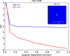 |
Fig. 1 Final results of the Gemini North speckle imaging of TOI-1438. The blue and red curves show the 5 σ contrast curves in 562 nm and 832 nm filters, respectively, as a function of the angular separation out to 1.2". The inset shows the reconstructed 832 nm image with a 1" scale bar. TOI-1438 was found to have no close companions from the diffraction limit out to 1.2" and within the magnitude contrast levels achieved. |
2.4 Radial velocity follow-up with HARPS-N
Within the KESPRINT consortium program, we observed TOI-1438 with the high resolution spectrograph HARPS-N (Cosentino et al. 2014) mounted on the 3.58-m Telescopio Nazionale Galileo (TNG) of Roque de los Muchachos Observatory in La Palma5 covering wavelengths between 378 nm and 691 nm at a spectral resolution of R ≈ 115 000. We followed this target between 17 March 2020 and 15 March 2025 collecting 85 RVs with exposure times of 1500-3300 s and an average signal-to-noise ratio (S/N) of 51 at 550 nm. We reduced the data through the Yabi web application (Hunter et al. 2012)6 running the offline version of the HARPS-N data reduction software (DRS) and choosing a K5 mask template and a crosscorrelation function (CCF) width of 30 kms−1 with a step of 0.25 kms−1. The HARPS-N absolute RVs measured with the DRS have uncertainties in a range 0.9-5.6 m s−1 with a median value of 1.6 m s−1 and an RMS of 22.2 m s−1 about the mean value. We measured the differential line width (dLW), Hα, NaD1, and NaD2 indexes with the Serval (Zechmeister et al. 2018) code and the template matching technique. The HARPS-N relative RVs measured with Serval have uncertainties in a range 0.9-3.7 m s−1 with a median value of 1.4 m s−1 and an RMS of 22.3 m s−1 about the mean value. All the RV measurements together with activity indicators from DRS and Serval are available online (see data availability).
Comparison of spectroscopic parameters of TOI-1438 derived by different methods.
2.5 Radial velocity follow-up with HIRES
We collected 20 spectra with the High Resolution Echelle Spectrometer (HIRES; Vogt et al. 1994) at the Keck Observatory over two years. With a resolving power of ≈60000 and wavelength range from 374-970 nm, HIRES provided precision RVs with a median uncertainty of 1.7 m s−1 from spectra with an S/N of 150 for TOI-1438. The RMS of the HIRES RVs is 18.9 m s−1 about the mean value. Using the iodine technique (Butler & Marcy 1996) and the standard California Planet Search setup and RV extraction technique (Howard et al. 2010), the RVs were combined with other RV datasets with an additional offset parameter in the RV model. A survey-wide assessment of HIRES RVs of TESS targets, including tOi-1438, can be found in Polanski et al. (2024) and the results in Van Zandt et al. (2025). The HIRES RVs are available online (see the second on data availability).
3 Data analysis
3.1 Stellar properties
We used the empirical code SpecMatch-Emp (Yee et al. 2017) that compares the observed optical spectrum with a dense library of well-characterised stars to analyse the coadded high-resolution HARPS-N spectrum. We then proceeded with more detailed modelling using Spectroscopy Made Easy7 (SME; Valenti & Piskunov 1996; Piskunov & Valenti 2017), a software that fits observations to computed synthetic spectra. We chose the MARCS stellar atmosphere grid (Gustafsson et al. 2008), retrieved atomic and molecular line data from VALD8 (Ryabchikova et al. 2015), and used the output from SpecMatch-Emp as initial values in the modelling. We followed the procedure in Persson et al. (2018) modelling one parameter at a time. The micro- and macro-turbulent velocities were kept fixed to 0.8 kms−1 (Bruntt et al. 2010) and 2.5 kms−1 (Doyle et al. 2014), respectively. The final results are tabulated in Table 2 and are in good agreement with SpecMatch-Emp matching a typical K0V star. The effective temperature and surface gravity are also consistent with Gaia DR3 which, however, report a lower iron abundance.
In order to derive an empirical measurement of the stellar radius, we used the ARIADNE9 (Vines & Jenkins 2022) software to perform an analysis of the broadband spectral energy distribution (SED) of the star together with the Gaia DR3 parallax and the SME results as priors. The SED was fitted based on four atmospheric model grids, Phoenix v2 (Husser et al. 2013), BtSettl (Allard et al. 2012), Castelli & Kurucz (2004), and Kurucz (1993), to the observed broadband photometry bandpasses G, GBP, and GRP (Gaia DR3), the Johnson B and V magnitudes (APASS), the infrared JHKs magnitudes (2MASS) and W1-W2 magnitudes (WISE) listed in Table 1. An upper limit on the visual extinction, AV, was obtained from the dust maps of Schlegel et al. (1998). A weighted average of the stellar radius was computed with Bayesian model averaging based on the relative probabilities of each model. The SED model is shown in Fig. 2. The luminosity becomes 0.45 ± 0.02 L⊙ and the extinction is consistent with zero (AV = 0.04 ± 0.05). The stellar mass is also modelled with ARIADNE based on the MIST (Choi et al. 2016) isochrones and the output from the SED model. The results are listed in Table 3.
To check the derived stellar parameters, we used the online applet PARAM1.310 (da Silva et al. 2006) with the SME spectroscopic parameters as priors, the Gaia DR3 parallax and the apparent visual magnitude, along with the PARSEC (Bressan et al. 2012) isochrones. Finally, we also compared our results with the Torres et al. (2010) calibration equations computed with the ARIADNE posterior spectroscopic parameters.
The results of the different models are listed in Table 3 with the corresponding stellar densities, which are used to constrain our transit model in Sect. 3.4 and comparison values of a typical K0V star. The values are in excellent agreement and we chose the ARIADNE results as our final adopted values also listed in Table 1. Some key stellar parameters required to obtain the absolute planet radii and masses from the transit and RV modelling, as well as the instellation and equilibrium temperature, are also listed in Table 5. Our derived stellar parameters are also in excellent agreement with the values listed on the EXOFOP-TESS website.
The age of a main sequence star such as TOI-1438 is often very difficult to estimate accurately. We obtained ages of 4.2 ± 1.5 Gyr with SpecMatch-Emp, 5.9 ± 4.2 Gyr with PARAM1.3, and  Gyr with ARIADNE based on the MIST (Choi et al. 2016) isochrones. Based on the derived projected rotational period, Prot∕ sin i⋆, in Sect. 3.2 and different gyrochronology (rotation-age) relations (Barnes 2007; Mamajek & Hillenbrand 2008; Angus et al. 2019; Mathur et al. 2023), we obtained ages from 1.8 to 5.4 Gyr. Finally, we also estimate the age using the magnetochronology relations from Mamajek & Hillenbrand (2008). This relation, combined with our mean value of log (R′HK) = −4.925 ± 0.013 (Sect. 3.3) results in an age range from 5.0 to 5.5 Gyr. Thus, the different estimates points to an age between ~2 and 6 Gyr.
Comparison of stellar mass and radius of TOI-1438 derived by different methods compared to values of a typical K0V star.
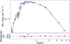 |
Fig. 2 SED of TOI-1438 and the model with highest probability (Castelli & Kurucz 2004) are plotted together with the synthetic photometry (magenta diamonds) and the observed photometry (blue points). The vertical error bars outlines the 1 σ uncertainties and the horizontal bars the effective width of the passbands. The residuals of the fit (normalised to the errors of the photometry) are shown in the lower panel. |
3.2 Stellar rotation period
We computed a first estimate of the projected rotation period, Prot/ sin i⋆ from the spectroscopic V sin i⋆ together with R⋆ and obtained Prot/ sin i⋆ = 22.8 ± 11.4 d. Given the large error bars and the unknown value of i⋆, we proceeded with an analysis of the TESS photometric data.
For the analysis of stellar rotation in the TESS light curves, especially for long rotation periods, it is crucial to preserve low-frequency stellar signals. Unfortunately, the PDCSAP flux includes filtering and CBV corrections that removes systematics, which can also eliminate long stellar rotation variability. Thus, we used SPOC (Twicken et al. 2010; Morris et al. 2020) light curves as well as Quick Look Pipeline (QLP, Huang et al. 2020a,b; Kunimoto et al. 2022) SAP_FLUX data to investigate the signature of the stellar rotation. This implies that particular caution is required, as the long-period variability observed in TOI-1438 may be significantly affected by TESS systematics, as seen in Sector 74. Exoplanet analyses rely on PDCSAP light curves, which are optimised for high-frequency signals; this approach allows the inclusion of a larger amount of data, as low-frequency variability is not critical for such studies.
Starting with 38 TESS sectors, we built light curves with a 30-min cadence, where the gaps between sectors (longer than 1 yr) have been removed, assigning to the first cadence of the new campaigns the time of the last cadence of the previous campaign plus 30 min. This is justified because we expect active regions to lose coherence during gaps of one to two years (for intensive tests on TESS-like observations see, García et al. 2024). Moreover, to enable a reliable analysis of rotation periods up to 30 days, we required the use of segments of continuous TESS data spanning at least 90 days. Hence, we independently analysed chunks of continuous sectors (for example sectors 14-21, 23-26, 47-51, and so on) and removed the sectors dominated by TESS systematics, such as sectors 57 and 74.
For all of the datasets, we tried different stitching methods (Palakkatharappil et al. 2024) by using the mean of the sectors, the mean of half sectors, fitting different polynomials at the end and beginning of the continuous sectors, finding the middle point of the gap, and looking for the offset as done in García et al. (2011). We also combined the different methods using Bayesian techniques as done in Handberg & Lund (2014), using the pyTADACS pipeline (under development, García et al. 2024). For all these light curves, we interpolated the gaps using a multiscale discrete cosine transform following inpainting techniques (García et al. 2014; Pires et al. 2015).
We applied different methods on the resulting light curves to search for the stellar rotation period: periodogram, timefrequency analysis with wavelets (e.g. Torrence & Compo 1998; Mathur et al. 2010), the auto-correlation function (e.g. McQuillan et al. 2013), and the composite spectrum that is a combination of the wavelet power spectrum and the ACF (Ceillier et al. 2017). These different methods in our rotation pipeline enabled us to find the most reliable rotation periods (Aigrain et al. 2015). This procedure was successfully applied to the Kepler data (Santos et al. 2019, 2021) providing a catalog of more than 55 000 rotation periods.
However, the analysis of the various TESS light curves of TOI-1438 did not yield a reliable rotation period. Modulations with periods of approximately 14 and 27 days were detected most of the time that correspond to the sector and half-sector periodicities suggesting that we were not able to properly detrend the light curves. Only the analysis of the first continuous segment (sectors 14-21) yielded a possible rotation period of 23.0 ± 1.4 d (obtained from the wavelet analysis), which does not seem to be due to any instrumental effect. We want to emphasise that only small gaps were interpolated in this segment. Given that the TESS observations span more than 5 yr, it is possible that this could be due to changes in the magnetic activity cycle of the star.
Thanks to the ground-based follow-up of this star providing the activity index R′HK from the Ca II H & K lines (see Sect. 3.3), we checked the magnetic activity level of the star during the TESS observations. We found that the TESS sectors where the overall variance of the light curve is larger (which could be related to a larger activity, e.g. Salabert et al. 2016) correspond to a high level of surface magnetic activity retrieved from R′HK. This suggests that the low-frequency modulation we see in the TESS light curves could be of magnetic origin related to activity. A longer, continuous dataset is required to obtain a reliable Prot for this star.
The preliminary value of 23.0 ± 1.4 d is, however, in agreement with the rotation period computed from R⋆ and V sin i⋆. Assuming that the value derived from TESS photometry is robust, we estimated the stellar inclination from the rotation period in combination with the spectroscopically derived V sin i⋆ and R⋆ following Masuda & Winn (2020). Using V sin i⋆ = 1.8 ± 0.9 kms−1, R⋆ = 0.820 ± 0.017 R⊙, and Prot = 23.0 ± 1.4 d, the stellar inclination becomes  . This is consistent with the picture of a well-aligned system.
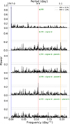 |
Fig. 3 GLS periodogram of the HARPS-N and HIRES RV data. The GLS of the raw RVs are shown in the top panel and the below panels have the best-fitting models subtracted for a given planet or signal d, as described in Sect. 3.4. From right to left, the orange, red, and blue vertical lines denotes the orbital periods of planets b and c, and signal d, respectively. |
3.3 Frequency analysis of the RVs and activity indicators
We performed a frequency analysis of the HARPS-N time series data to search for signals from the planets and the host star in the RV measurements and activity indicators. Figure 3 shows the generalised Lomb-Scargle (GLS; Zechmeister & Kürster 2009) periodograms of the HARPS-N and HIRES RVs. The false alarm probabilities (FAPs) were computed using the bootstrap technique (Kuerster et al. 1997). A peak is considered to be significant if its FAP < 0.1%. In the top panel of Fig. 3, we show the periodogram of the raw RVs, which clearly displays a longperiod signal marked with a blue vertical line which we hereafter refer to as signal d. The origin may be a wide orbiting, massive companion, either (sub-)stellar or planetary.
We subtracted our best fitted model of the long-period signal of 2767 d (see Sect. 3.4 and Table 5) and plot the resulting periodogram in the second top panel, revealing two peaks at the orbital periods of planets b and c (5.1 and 9.4 days, respectively) found in the transit data, marked by vertical red and orange lines. Further below we show the periodograms after also subtracting the best-fitted model for planet c and b in the third and fourth panels, respectively, where the signals of planets b and c are significantly detected in respective plot. Residuals after subtraction of both planets and signal d are plotted in the bottom panel.
Figure 4 shows the GLS periodograms of several activity indicators. No signals are detected at the orbital periods of planet b or c, hence we focus the figure on the short frequencies since a long-period signal of the order of thousands of days (similar to signal d) is seen in several of the activity indicators. We mark the orbital period of signal d with a vertical blue line for comparison, as well as the preliminary stellar rotation period of 23 days and Earth’s orbital period of 365 days with red and green vertical dashed lines, respectively. The long-period signal is most prominent in the S-index, dLW, CCF contrast, and NaD1.
A counterpart to the RV signal in the activity indicators would typically suggest that this phenomenon is of stellar origin, possibly stemming from long-period magnetic cycles. The longperiod peak in NaD1, however, coincides with Earth’s orbital period (0.00274 days−1) which suggests contamination by telluric features in this activity indicator. A correlation plot of RV against dLW is shown in Fig. A.1 which may suggest that dLW is ~90° out of phase, hence possibly anti-correlated with RVs.
Subtracting the long-period signal d of 2767 d from the S-index, dLW, and CCF contrast does not remove the signal or reveal the stellar rotation period. This may indicate that there are several long-period signals. However, the exact periodicity of the signals is difficult to determine, as the baseline is only 1824 d and thus the signals are not resolved at low frequencies.
We searched for chromatic changes in the RVs to rule out a planetary origin of signal d. If signal d is due to an orbiting planet, it should not be chromatic but consistent across different wavelength ranges. This is supported by the non-correlation of the CRX, defined as the RV gradient as a function of wavelength, with RVs shown in Fig. A.2. In addition, we extracted the RVs from the HARPS-N spectra from different parts of the spectra; “blue” (387.5-455.7 nm), “yellow” (453.9-549.3 nm) , and “red” (548.2-691.1 nm) wavelengths. Signal d was seen in the RVs extracted from all three wavelength ranges and was consistent with that observed from using the whole wavelength range supporting a planetary origin.
The TOI-1438 system may thus have an outer planet that induces the variation seen in the RV data as well as a long-term stellar magnetic cycle as detected in the activity indicators, but with negligible effects on the RVs. This scenario is supported by the large semi-amplitude K and the fact that TOI-1438 is not a very active star in addition to our analysis of the RV jitter in Sect. 4.2.
Compared with other solar-like stars from the Mount Wilson survey (Wilson 1978; Baliunas et al. 1995), a cycle period of about 2000 days would put the star on the active branch. When searching for signs of activity in the co-added HARPS-N spectrum, we identified only weak emission in the line cores of the Ca II H & K absorption lines shown in Fig. 5. Furthermore, the average Ca II chromospheric activity index log(R′HK) is −4.925 ± 0.013, which is comparable to the Sun at minimum activity (Mamajek & Hillenbrand 2008; Boro Saikia et al. 2018).
However, since we cannot rule out stellar activity as a possible origin of signal d with certainty, the planetary nature of signal d cannot be confirmed and remains a tentative discovery. More observations over a longer period of time is required to resolve the issue and disentangle the signals.
We also searched the TESS light curves for transits originating from this potential planet without success. The expected time of mid-transit seems to fall at a time where TESS was not observing this system. Furthermore, assuming coplanarity with planets b and c, the impact parameter of planet d would be >30, clearly suggesting that transits cannot be detected.
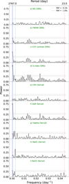 |
Fig. 4 GLS periodogram of HARPS-N data with activity indicators from DRS and Serval as indicated in the legends. The preliminary stellar rotation period of 23 days and Earth’s orbital period of 365 days are marked with red and green vertical dashed lines, respectively, and signal d with a blue vertical thick line. |
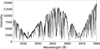 |
Fig. 5 Emission in the line cores of the Ca II H & K absorption lines in the co-added HARPS spectrum of TOI-1438. |
3.4 Joint transit and radial velocity modelling
We modelled the TESS light curves using the batman package (Kreidberg 2015) to extract information on the orbital period (P), the mid-transit time (T0), the planet-to-star radius ratio (Rp/R⋆), the scaled orbital separation (a/R⋆), and the orbital inclination (i) of both transiting planets. Despite the wealth of TESS photometry for this system, the transits are quite shallow and have a high impact parameter (b = cos i × a/R⋆), which entails that some parameters are difficult to constrain. Following Seager & Mallén-Ornelas (2003), we therefore constrained a/R⋆ by a Gaussian prior on the stellar density derived from our spectral analysis.
To account for photometric noise (instrumental and stellar) that might skew the estimation of the transit parameters, we detrended the light curves before fitting using Gaussian Process (GP) regression utilising the celerite library (Foreman-Mackey et al. 2017). We used a Matérn-3/2 kernel for our GP which is characterised by two hyperparameters; an amplitude (A) and a timescale (τ). This was done in an iterative manner, where we subsequently used the best-fitting transit parameters to filter out the transits when detrending. The detrended light curves for all TESS sectors are shown in Fig. 6. During fitting, we only included data in an interval with pre-ingress and post-egress around each mid-transit time.
We modelled the RVs as a sum of Keplerian orbits (e.g. Murray & Correia 2010) to obtain information on the RV semiamplitude (K) and, hence, the masses of the planets, as well as the orbital eccentricity (e) and argument of periastron (ω). We extracted the HARPS-N RVs from the DRS pipeline and Serval. The results from using either set of RVs were fully consistent with a slightly lower RMS for the DRS RVs, and we thus chose to use these in the joint transit and RV analysis.
Modelling stellar activity through the use of multidimensional GP regression can significantly improve the orbital parameters (e.g. Rajpaul et al. 2015; Barragán et al. 2022). This can be done by simultaneously modelling both the RVs and the activity indicator(s) displaying the signal with a quasi-periodic (QP) kernel (see, e.g. Eq. (15) in Aigrain & Foreman-Mackey 2023) with hyperparameters describing the characteristic period (λ1), the harmonic complexity (Γ), and the decoherence timescale (λ2). However, as pointed out by Barragán et al. (2022), QP kernels should only be used in cases where the periodicity is smaller than the decoherence timescale (i.e., λ1 < λ2), which in the present case constitutes a problem. This is because the periodicity of the signal seems to be longer than the baseline of the observations and is difficult to constrain. Obviously, it is therefore even more difficult to constrain the decoherence timescale in this case. Indeed, using the software pyaneti11 (Barragán et al. 2019, 2022), where we included the RVs and the dLW time series, we confirmed that it is not possible to constrain λ1 or λ2 without applying rather restrictive priors which goes against what we were trying to achieve by using multidimensional GPs, i.e. letting the data inform us. We were further able to confirm what is also evident from Fig. 7, namely that the harmonic complexity of this signal is very low, and it can therefore be exactly described by a sinusoid as discussed in Serrano et al. (2022).
Given the low harmonic complexity, we decided to model the RVs as three Keplerians: one for each transiting planet and one for the long-period signal, regardless of the origin of the signal (planet or stellar activity). We therefore proceeded without the inclusion of GPs and used our custom wrapper (i.e. the batman light curve and N Keplerian model as outlined above) instead of pyaneti. In order to investigate if an even simpler model for the long-term trend is preferred, we also tested a model including two Keplerians and a quadratic trend. We find that the Bayesian information criterion (BIC) favours a three Keplerian model over a quadratic trend (∆BIC = −47).
The posterior distributions for the parameters were sampled through Markov chain Monte Carlo (MCMC) sampling through the emcee code (Foreman-Mackey et al. 2013). The MCMC was initialised with 100 walkers with a 150 000 steps each. The walkers were initialised with half of them starting in a tight Gaussian ball around the best-fitting solution where the standard deviation is of the order of the uncertainty of the posterior for each parameter. The other half were spread uniformly across the allowed range. Convergence was assessed by calculating the rank normalised R diagnostic12 and visually inspecting the chains in a corner plot (Foreman-Mackey 2016). When fitting for the eccentricity, we stepped in  and
and  , and cos i instead of i. Furthermore, we used a quadratic limbdarkening law, where we stepped in the sum (q+ = q1 + q2) of the parameters to which we applied a Gaussian prior with a width of σ = 0.1, while keeping the difference (q- = q1 – q2) fixed. At each step in q+ we thus calculated q1 = (q+ + q-)/2 and q2 = (q+ – q-)/2. The starting points for q 1 and q2 were estimated by querying the table by Claret (2018).
We tested if any of the three signals displayed an appreciable amount of eccentricity and the potential influence on the inferred parameters, especially the orbital period of planet d. We began by making a model only including photometry to constrain P and T0 for the two transiting planets. Those values were used as priors in the subsequent models only including RVs where we first did a run fixing the eccentricity to zero for all three Keplerians. In this case, the period for planet d came out to P = 1798+82 d with a K-amplitude of  m s−1 meaning that with our 5 yr baseline we barely covered the whole cycle of signal d. We then compared this to a model in which we allowed
  and
and  to vary for all three. From this we found that the eccentricities for planets b and c from this run were consistent with zero (
 and
and  ). Moreover, we found a strong correlation between the orbital period and the eccentricity for planet d where a tail extending beyond e = 0.5, P = 5000 d, and K = 40 m s−1 is present in the posterior.
This implies that with the RV data currently in hand, we cannot constrain the eccentricity of signal d very well. However, although these eccentric, long-period solutions could be consistent with the data, they suggest that the 5 yr (1824 d) of RVs we have collected so far, were all acquired when planet d was close to periastron. During this 5 yr time span, we would in this case observe a large increase and decrease of 60 m s−1 in the RVs, while in the remaining 13 yr part of the orbit, the change in RVs would only be about 20 m s−1 . Such a scenario would mean we have have observed the system at a special time. This effect is even more pronounced for longer periods and more eccentric solutions. Although it is not impossible that we observed this system at epochs where it undergoes the most dramatic changes, it is unlikely. Furthermore, the eccentric solutions is to a large extent driven by the two most recent observations as the posteriors before obtaining these last two RVs did not have these highly eccentric tails for planet d. Particularly the most recent datum in Fig. 7 is seen to be the lowest observed RV yet. Finally, the quality of the derived orbit naturally depends on the number of cycles that has been covered (Zakamska et al. 2011), which presently in a best-case scenario for planet d means that we have only covered one cycle. Taken together we believe these arguments suggest that the eccentricity of planet d should be more modest. Rather than setting ed = 0, we applied a prior to ed using the Beta-distribution from Kipping (2013) with α = 0.867 and β = 3.03. Applying this Beta-prior gives a period of 2767-556 d (≈  years) for signal d.
In the following when we fitted the photometry and RVs jointly, we therefore proceeded with the setup where we applied a Beta prior to ed. In order to investigate the eccentricities for planets b and c, we ran two MCMC models summarised in Table 4: (i)  and
and  sin ω were allowed to vary for both planets b and c, and (ii) with fixed eccentricities, eb = ec = 0. The eccentricities in model (i) came out to eb =
  and ec =
  , which again means that the orbit for planet b is completely consistent with being circular while a slightly eccentric model for planet c seems to be favoured. The resulting K -amplitudes and masses along with eccentricities for the two models are listed in Table 4. The results are fully consistent within the uncertainties. From a dynamical point of view (Sect. 3.5) stable solutions are generally found for small eccentricities. Together with the fact that we find the eccentricity for planet b to be consistent with zero and only a very moderate eccentricity for planet c, we adopt model (ii) in which the eccentricities for planets b and c were fixed to zero as our final run as we believe this to be the more conservative and simpler approach. Finally, we investigated the consequences of applying a different prior on ed, namely the “Rayleigh+Exponential” suggested by Stevenson et al. (2025), which is based on an updated sample of exoplanet eccentricities. The results of model (i) and (ii) with a “Rayleigh+Exponential” prior for planet d were fully consistent with each other, and also with a Beta prior on planet d.
The final best-fitting transiting models for planets b and c are shown in Fig. 6 and the best-fitting Keplerians are shown in Fig. 7. We tabulate the posterior values in Table 5 and show corner plots of the posterior distributions in Figs. A.3-A.5.
The results stemming from the procedure outlined above was obtained using our own software. As an independent check, we modelled the photometry and RVs with pyaneti (Barragán et al. 2019, 2022), and a similar setup (i.e. a three-Keplerian model with a Beta-prior applied to ed) resulted in fully consistent parameters.
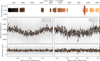 |
Fig. 6 TESS photometry of TOI-1438. Top: the de-trended TESS time series colour-coded according to sector; from black in Sector 14 to light copper in Sector 81. The data from Sector 74 is under the red cross and was excluded from the analysis. In total, there are 150 and 79 transits of planets b and c, respectively (excluding Sector 74). Middle: the phasefolded light curves for planets b (left) and c (right). The unbinned data are shown as small, grey markers, and the larger markers are ~10 min binned data colour-coded as in the top panel. The best-fitting models are shown as the white lines. Bottom: residuals from subtracting the best-fitting models from the data. |
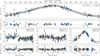 |
Fig.7 RVs of TOI-1438. Top: the HARPS-N (blue) and HIRES (orange) RV time series with the best-fitting three Keplerian model in grey with residuals shown in the panel below. Lower: the phasefolded RV curves for planet b (left) and c (middle) as well as signal d (right). The best-fitting models are shown as the grey lines with the shaded area denoting the 1 and 2 σ intervals in the K-amplitude. Residuals are given below. |
Summary models of planets b and c with free (model i) and fixed eccentricities (model ii).
3.5 Dynamical analysis
The influence that outer giant planets are expected to have on the orbital dynamics, especially the coplanarity, of inner transiting planets has been extensively studied (Boué & Fabrycky 2014; Becker & Adams 2017; Lai & Pu 2017; Mustill et al. 2017; Poon & Nelson 2020; Rodet & Lai 2021; Livesey & Becker 2025). In the case of the TOI-1438 system, given the proximity of the orbits of the innermost fairly massive planet to the 2:1 MMR region, the system may be dynamically active, primarily driven by the two mini-Neptunes. Any influence of the outer planet can likely be attributed to very long-term secular effects. We have therefore focused on the short-term dynamics.
The parameter space can be reduced to essentially three variables: the eccentricities forming a plane (eb, ec) and the difference of the periastron arguments Δϖ = ωc − ωb, as the third dimension. In close in-systems, which are likely to have undergone inward migration, we can expect the most likely “slices” ∆ϖ = 180° or, depending on migration conditions, also Δϖ= 0° (e.g. Papaloizou & Szuszkiewicz 2005; Hadden & Payne 2020; Xu & Fabrycky 2019; Deck & Batygin 2022; Cresswell & Nelson 2022; Mills et al. 2023). We also considered intermediate cases Δϖ = 90° and 270°, consistent with the best-fit values found in experiments with eccentricities as free parameters (Sect. 3.4). Using this parametrisation, we can capture the essential features of the dynamics of the system by fixing relatively well-determined masses, inclinations, orbital periods, and mean anomalies at the epoch based on photometry data and further constrained by the joint RVs model. The eccentricity and pericentre arguments are allowed to vary as they have the largest uncertainties, reflecting the nature of the RV data.
To assess the dynamical stability of the solutions, we used the reversibility error method (REM; Panichi et al. 2017), which has been shown to be a close analog of the maximum Lyapunov exponent (MLE) and the well known indicator MEGNO (e.g. Gozdziewski et al. 2001; Cincotta et al. 2003). In the analysis of multiple systems, the REM indicator relies on numerical integration schemes that are time-reversible, in particular symplectic algorithms. This method is based on the calculation of the difference between the initial state vector and the final state vector obtained by integrating the Newtonian equations of motion for a given interval and then returning to the initial epoch by integrating the system back for the same time. The difference depends on the dynamical nature of the system. REM = 1 or log REM = 0 means that the difference reaches the size of the orbit. For regular (stable) orbits, REM grows with polynomial rate with time, and for chaotic (unstable) solutions it grows exponentially. The fast indicator is crucial for illustrating the phase space of the system, since it detects instability much faster than direct numerical integration could do.
We tested the dynamical stability of the solutions constructed around the nominal value of the best-fitted parameters from model (i) in Sect. 3.4 in the (eb, ec) plane for fixed, representative values of ∆ϖ. We integrated the orbits with the whfast integrator, the 17th-order corrector, and a fixed time step of 0.04 d as implemented in the REBOUND package (Rein & Liu 2012; Rein & Spiegel 2015) for 50 000 orbital periods of the second planet. Such a timescale is sufficient to detect short-term MMR-driven dynamics (Panichi et al. 2017).
The results are shown in Fig. 8. Subsequent panels are labeled with ∆ϖ, which is fixed in the given simulation. A black curve marks the collision curve of the orbits. The orbits can mutually cross already for moderate eccentricities and long-term stability of the system is possible only in some regions of the (eb, ec)-plane. In all cases, the nominal system with ec ≃ 0.16 is close to the very edge of collision zone and becomes unstable. Furthermore, it is clear that the size of this zone and its shape depend strongly on the initial relative orientation (∆ϖ) of the orbits.
We can also show that the REM signature of stability is closely reflected by the geometric evolution of the orbits. This is illustrated with some examples in Fig. 9. The top panel is for a low eccentricity solution, which is in the stability zone. The middle panel is for moderate eccentricities eb = 0.1, ec = 0.2 and ∆ϖ = 90° (near the origin), the system is still strictly stable.
The last panel shows a chaotic solution where the eccentricity reaches the collision zone, such a system is unlikely to survive long-term evolution.
The system does not seem to be involved in a strong, low-order resonance, as we have verified with additional direct integrations. Then the likely origin by convergent migration and the final proximity of the planets to the star would also be consistent with low eccentricities due to tidal damping.
To verify this hypothesis more deeply on dynamical grounds, we simulated the range of TTVs for the inner pair (Fig. 10), setting the same (eb, ec) plane and other parameters as in the dynamical maps in Fig. 8. Obviously, for eccentric systems, the TTV range could be as large as ≃3 hours and easily detectable in the available set of light curves. However, this is not the case. Using PyORBIT (Malavolta et al. 2016, 2018) we have measured the TTVs for all light curves in all available TESS sectors (Fig. 11). In top of the strong noise, the measured TTV amplitude remains at the level of a few minutes with a large spread, making the detection of TTVs useful in orbital fitting practically impossible, despite (possibly) being a prior for dynamical RV modelling.
Curiously, the simulated TTVs closely follow the structures in the REM map. In one case (top left panel, for ∆ϖ = 0°) there is a diagonal band of small TTVs across all the eb ≃ ec. However, in this region, the systems are stable only for small and moderate eccentricities, below the collision curve, hence only a corresponding triangular area in the TTV band is dynamically permitted. We illustrate this further with the TTV contours over-plotted on the REM maps (Fig. 8) to guide the eye. The correspondence of the two dynamical characteristics is striking and for any tested ∆ϖ, they overlap only in the region of small eccentricities.
Moreover, in such a case, the Keplerian RV model applied here remains valid, since the differences in the RV signals between Keplerian and N-body models reach 1 ms−1 after 5 years of observations. Overall, our experiments support low-eccentricity orbits in the lower bound of ec, confirming the results of the analysis described in Sect. 3.4.
Given the complex and active system described above, a detailed dynamical analysis of its state is beyond the scope of this present paper. New RV observations would be crucial to constrain the inner eccentricities and orbital elements of the outermost Jovian companion (especially its period) and allow us to infer hypothetical low-mass planets in the apparently empty zone between the inner subsystem and this giant planet.
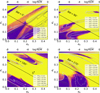 |
Fig. 8 Dynamical maps of the eccentricities of the two inner planets (eb, ec) and fixed values of the argument of pericentre of TOI-1438 b(∆ϖ = ωc − ωb). The black filled circle with a white rim shows the location of the solution obtained by modelling with the eccentricities set as free parameters. Small values of the fast indicator log REM characterises regular (long-term stable) solutions, which are marked with black and dark blue colour. Chaotic solutions are marked with brighter colours, up to yellow. The black line represents the so-called collision curve of orbits, defined by the condition: αb(1 + eb) = ac(1 − ec). The resolution of each plot is 301 × 301 points. Triangles marked 1-3 correspond to the solutions shown in Fig. 9. Also, the labelled grey contours refer to the TTV amplitudes shown in Fig. 10 (details in Section 3.5). |
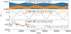 |
Fig. 9 Temporal evolution of eccentricities for the representative solution selected in the dynamical maps shown in Fig. 8. The eccentricity of TOI-1438 b and TOI-1438 c are marked in blue and orange, respectively. |
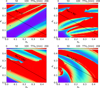 |
Fig. 10 TTV amplitudes in the (eb, ec)-plane and fixed initial values of the argument of pericentre TOI-1438 b (∆ϖ = ωc − ωb), computed for the RV data time span. The black filled circle with a white rim shows the location of the solution obtained with a model where the eccentricities are set as free parameters. |
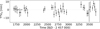 |
Fig. 11 TTV measurements based on the TESS photometric data (and spanning all but two sectors) skipped due to excessive noise. |
4 Discussion
4.1 Interior structure models for planets b and c
Figure 12 plots all planets from the NASA exoplanet archive with uncertainties better than 21% and 7% in mass and radius, respectively, as of 12 April 2025. The uncertainties are chosen to have the same impact on the bulk density. Also shown are brown dwarfs (Table A.1 in Barkaoui et al. 2025, and references therein), and eclipsing low-mass stars (Ribas 2003; Bouchy et al. 2005; Pont et al. 2005, 2006; Demory et al. 2009; Tal-Or et al. 2013; Zhou et al. 2014; Díaz et al. 2014; Chaturvedi et al. 2016; Gillen et al. 2017; von Boetticher et al. 2017; Shporer et al. 2017; Chaturvedi et al. 2018; Carmichael et al. 2019; Grieves et al. 2021; Vowell et al. 2025; Barkaoui et al. 2025, and references therein). TOI-1438 b and c nicely fall within the diagonal strip of (sub-)Neptunes which displays decreasing density with increasing radius. The derived masses in this plot are mainly from RVs, but also from TTVs outlined in dark grey. Sub-Neptunes characterised by TTVs are puffier with lower densities compared to the bulk of the RV-characterised population of sub-Neptunes clearly seen in Fig. 12. This suggests that resonant planets have retained their lower initial density as compared to non-resonant sub-Neptunes (Leleu et al. 2024). The radius gap that separates rocky super-Earths with volatile sub-Neptunes (Fulton et al. 2017; Fulton & Petigura 2018) is seen between the water-rich and silicate interior composition models.
To determine the planetary structure and composition of TOI-1438 b and c, we performed an interior retrieval using the mass-radius table from Aguichine et al. (2021) as our initial approach. This table was calculated by assuming a three-layered structure: a Fe-rich core, a silicate mantle, and an irradiated water envelope. This interior model assumes hydrostatic equilibrium, conservation of mass, Gauss’ theorem for the computation of gravity, and convection as the main heat transport mechanism. The density calculations use the Vinet equations of state (EOS) for iron and rock (details in Brugger et al. 2016; Brugger et al. 2017) and Mazevet et al. (2019) for water under conditions exceeding the critical point. An atmospheric model provides the boundary conditions for pressure and temperature, adopting a wet/dry adiabatic profile near the surface and an isothermal mesosphere at low pressures. The atmosphere is heated by the stellar irradiation from the top isotropically, and internal heat sources coming from the interior are neglected.
The forward model incorporates four input parameters defined with their priors in Table 6. The Fe-to-refractory mass ratio, our first parameter, represents the core mass fraction (CMF) divided by the combined mass of the core and mantle (the sum of CMF and mantle mass fraction, MMF). The mantle and core together form the planet’s refractory component (rocks and Fe), while volatiles exist separately in the envelope. For reference, the Earth presents a CMF = 0.32, and MMF + CMF ≈1, yielding a Fe-to-refractory mass ratio of 0.32. Since water comprises the entire envelope, its mass fraction equals the water mass fraction (WMF).
We sampled the posterior using emcee and computed the likelihood function using the squared residuals of the observed mass and radius, according to Eqs. (6) and (14) in Dorn et al. (2015) and Acuña et al. (2021), respectively. For the MCMC retrieval, we used 32 walkers and N = 105 steps. The retrieval’s autocorrelation time was τ = 70 and 66 for planets b and c, respectively. The MCMC convergence criterion was τ ≪ N/50. In our case N/50 = 2000, showing that the chains are long enough to ensure convergence with the estimated autocorrelation times. We also ran retrievals assuming the mass values from different eccentricity models. The difference in WMF between these is less than 5 wt%, demonstrating that our conclusions on the interior composition of planets b and c are robust against differences in eccentricities.
The posterior distribution functions of our MCMC retrievals are shown in Fig. A.6. Table 6 shows the resulting mean and uncertainties of the posterior distribution functions. We observe that the retrieved Fe-to-refractory mass ratio spans CMF/(CMF + MMF) = [0.13, 0.73]. This range is wider than that reported in the super-Earth and hot rocky exoplanet population (Schulze et al. 2021; Liu & Ni 2023; Brinkman et al. 2024), which is CMFZ(CMF + MMF) ~ [0.20,0.46] (Plotnykov & Valencia 2020). Using only mass and radius measurements, we cannot effectively constrain the Fe-to-refractory ratio for sub-Neptunes. This is due to a change in CMF having a very small effect on radius compared to the volatile mass fraction, H/He and/or water, in sub-Neptunes and exoplanets with significant envelopes (see Otegi et al. 2020; Acuña Aguirre 2022, for a detailed discussion on this degeneracy).
We obtained well-defined 1σ estimates for WMFs of [0.67, 0.94] and [0.44, 0.75] for planets b and c, respectively. We report a mean WMF for planet b of ≈20 wt% higher than for planet c, although their WMFs are consistent within 1.2 σ. Given the current uncertainties, these planets might have comparable water mass fractions, or planet b may be marginally more water-rich. Distinguishing between these scenarios would require improving the planetary radii precision from 6% to 2%, which would reduce WMF uncertainties from 18 wt% to 9 wt% which is a twofold improvement in precision. While JWST offers sufficient precision for such radius measurements, the TSMs of both planets (Table 5) are below the recommended cut-off for subNeptunes (TSM > 90, Kempton et al. 2018). Nonetheless, the atmospheric characterisation of TOI-1438 b (TSM = 64), particularly the detection of H2O and CH4, may still be possible with a few transit observations, as suggested for planets with similar TSMs (Chaturvedi et al. 2022).
We used mass-radius curves by an interior structure model that makes two assumptions: volatile species have water-like densities and occupy an isolated envelope layer distinct from the mantle and core. However, actual planetary structures may be more complex. Recent JWST transmission spectra of subNeptunes reveal envelopes containing mixtures of HZHe and high-molecular-weight species (H2O, CO2, CO, CH4, NH3) at envelope metal mass fractions ~50% (Benneke et al. 2024; Holmberg & Madhusudhan 2024; Piaulet-Ghorayeb et al. 2024). In addition, rock mantles may be soluble and miscible with water and other volatiles (Kite et al. 2019; Vazan et al. 2022; Schlichting & Young 2022; Luo et al. 2024).
To demonstrate the degenerate nature of TOI-1438 b and c’s interiors as sub-Neptunes, we employed the open-source Python package GASTLI (GAS gianT modeL for Interiors, Acuña et al. 2021; Acuña et al. 2024) to generate forward interior structure models in Fig. 13. GASTLI models planetary structure using two distinct layers: a deep inner layer containing equal parts rocks and water by mass, and an outer envelope composed of H/He and water serving as a proxy for metals. GASTLI uses state-of-the-art EOS for rock, water and H/He. We couple it to its default atmospheric grid to calculate the envelope boundary conditions. This grid contains pressure-temperature profiles for warm (Teq < 1000 K) volatile-rich exoplanets generated with the self-consistent radiative-convective model petitCODE (details in Acuña et al. 2024).
Given the wide range of possible ages within 1 σ for TOI-1438 (Sect. 3.1) and that sub-Neptunes cool faster than their gas giant counterparts (Chen & Rogers 2016), we adopted an intrinsic temperature of Tint = 50 K. Fig. 13 shows that both planets could have a mixed interior of volatiles and rock, overlaid by a metal-rich, H/He envelope. In particular, planet b could have an envelope as massive as 0.5 M⊕, representing 5% of the planet’s total mass. Its composition ranges from an equal mix of H/He and metals to a high mean molecular weight atmosphere composed purely of metals. In contrast, planet c’s envelope is significantly less massive, <1% of its total mass, with a minimum envelope metal content of 80% by mass. External heat sources, such as tidal heating from non-zero eccentricity (Agúndez et al. 2014), would produce effects similar to increasing the H/He fraction in the envelope. Consequently, if internal heat sources are present, envelopes containing less than 20% H/He might be necessary to explain the observed masses and radii of both planets.
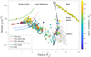 |
Fig. 12 Density vs radius diagram of the 230 planets in 159 multiplanet systems with ≥2 planets from the NASA exoplanet archive with uncertainties better than 21% and 7% in mass and radius, respectively, color-coded with instellation. The planets plotted in grey are single planet systems. The masses are derived from RV measurements (181 planets) or from TTVs (49 planets outlined in dark grey), and the radii from transit photometry. Solar System planets are marked with brown squares. Low-mass stars are marked with yellow star symbols. TOI-1438 b and c are marked with red star symbols and fall within the diagonal strip of (sub-)Neptunes which displays decreasing density with increasing radius. The interior models for low mass-planets are from Zeng et al. (2019), and the solid black line shows the interior model of H/He dominated giant objects with Z = 0.02, age = 5 Gyr, and no irradiation (Baraffe et al. 2003, 2008). |
Best fit compositional parameters, planetary masses, and equilibrium temperatures derived from our MCMC interior structure analysis.
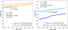 |
Fig. 13 Mass-radius relationships for TOI-1438 b (left panel) and c (right panel). The GASTLI interior structure models are flexible enough to incorporate an inner deep layer of equal parts rock and water (50% each), along with a H/He envelope containing variable metal content. We adopt an intrinsic temperature Tint = 50 K (see text) across all models. The observed masses and radii of TOI-1438 b and c support multiple possible interior configurations, from planets with Fe-rich cores and isolated irradiated hydrospheres to those with mixed rock-water interiors covered by envelopes of varying H/He and metal proportions. |
4.2 Signal d
If signal d is shown to be due to stellar activity, a striking feature of this signal would be the large amplitude of  m s−1 (or potentially higher, as explained in Sect. 3.4), especially considering that the star is not very active (log R′HK = −4.925 ± 0.013). To investigate if an amplitude of this magnitude is typical for stars with this activity level, we cross-matched the exoplanet hosts log R′HK values derived in Claudi et al. (2024) with the jitter (σ1) values from Bonomo et al. (2017), both based on observations with HARPS-N. In Fig. 14, we show stars appearing in both aforementioned studies with M⋆ < 1.1 M⊙ and at least ten RV observations. The light-grey error bars are systems with a baseline shorter than 1 yr, the black ones have a baseline longer than 2 yr, and the grey ones have baselines in between. To set TOI-1438 into this context, we fitted the RVs assuming a two-planet model (planets b and c) and let the jitter term absorb the long-period signal. The result was σ1 = 22.7 ± 1.8 m s−1, a rather large value among these stars as is evident from Fig. 14.
One aspect this plot obviously fails to convey is the complexity of the signal(s) responsible for the jitter. Signal d in TOI-1438 has a low harmonic complexity and can be nicely modelled as a simple Keplerian orbit. The figure also does not provide any information on the potential periodicity of the phenomenon. We therefore took a closer look at four of the systems closest to TOI-1438 in log R′HK − σ1 space, namely, HAT-P-15 (Teff = 5568 ± 90 K, log g = 4.38 ± 0.03; Kovács et al. 2010), HAT-P-18 (Teff = 4750 ± 100 K, log g = 4.50 ± 0.25; Hartman et al. 2011), WASP-10 (Teff = 4675 ± 100 K, log g = 4.40 ± 0.20; Christian et al. 2009), and TrES-4 (Teff = 6100 ± 150 K, log g = 4.045 ± 0.034; Mandushev et al. 2007). All four targets have been monitored with HARPS-N and/or HIRES and have baselines well over 1500 d (Knutson et al. 2014; Bonomo et al. 2017); however, the sampling for TOI-1438 is much better (105 RVs compared to at most 48 for HAT-P-18). We collected the RVs from these two studies, along with RVs for WASP-10 obtained with the SOPHIE and FIES spectrographs and looked at the residuals after subtracting the best-fitting models. Figure A.7 shows the residuals and their associated periodograms.
The morphology of the residuals from these four targets appear quite different from that of TOI-1438, as they do not seem to display any coherent signal on long timescales. Indeed, from calculating the GLS, the most prominent peaks had periodicities of 165 d or less. Moreover, the peaks in the periodograms do not have a FAP < 0.1%; therefore, they are not considered to be significant. We further note that for WASP-10, the jitter stemming from HIRES was significantly lower than that coming from SOPHIE and FIES. This is also quite apparent by eye and from the root-mean-square (RMSHIRES = 4.26 m s−1, RMSSOPHIE = 29.39 m s−1, RMSFIES = 47.73 m s−1). The large value reported for the jitter for this system might therefore be explained (at least partly) by instrumental noise. Taken together, we believe that the source of the jitter in TOI-1438 is inherently different in both morphology and periodicity compared to the other four systems. Overall, this supports a planetary origin of signal d. However, to confidently confirm the existence of planet d, we need more data over a longer baseline to resolve the long-period signals of stellar activity.
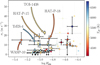 |
Fig. 14 RV jitter (σ1) as derived in Bonomo et al. (2017) as a function of log R′HK activity index calculated in Claudi et al. (2024) for exoplanet host stars with M⋆ < 1.1 M⊙. Light-grey error bars denote systems with a baseline shorter than 1 yr, grey error bars are systems with a baseline 1-2 yr, and black error bars are systems with baselines >2 yr. The error bars with arrows are upper limits on the RV jitter. The markers are colour coded with the stellar Teff. TOI-1438 is marked with a square. The marked systems HAT-P-15, HAT-P-19, TrES-4, and WASP-10 are discussed in Sect. 4.3. Adapted from Fig. 3 in Hekker et al. (2006). |
4.3 System architecture
The architecture of the TOI-1438 system is composed of an inner system with two sub-Neptunes and likely an outer system harbouring a giant planet. If a three-planet system, TOI-1438 belongs to a small group of detected systems with inner, small planets and outer long-period giant planets; for instance, Kepler-48 (Steffen et al. 2013; Marcy et al. 2014) and TOI-4010 (Kunimoto et al. 2023). To compare the architecture of TOI-1438 to all the detected systems so far, we selected systems from the NASA Exoplanet Archive that contain a minimum of three planets, with at least one confirmed small (R < 4 R⊕) or low-mass planet (M < 20 M⊕) with an orbital period < 10 days and an outer confirmed giant planet (R > 8 R⊕ or M > 90 M⊕) with P > 300 days. We applied the mass-radius relationships from Müller et al. (2024) to convert the measured masses to radii and vice versa for the planets that did not have both radius and mass values. There are only 26 systems that fulfill these criteria as of 12 April 2025, most of which do not display a large gap between the outer giant and its inner adjacent planet similar to TOI-1438, as visualised in Fig. 15. The largest orbital period ratio between two adjacent planets in each system is given in parentheses after each host star’s name and increases from top to bottom in the figure. It is clear that the TOI-1438 system has a unique architecture with two small, low-mass, and tightly packed planets orbiting close to the host star and a Jupiter-like planet residing in the outer region of the system separated from planet c by an orbital period ratio of ~300. Only one system, HD 153557 (Feng et al. 2022), has a larger orbital period ratio between the inner and outer system; however, the outer object is a brown dwarf, or possibly a low-mass star, with a minimum mass of 27 MJ.
Previous studies have shown that inner small planets in observed multi-planetary systems with outer giants tend to have more irregular orbital spacings than the planets in systems without any long-period giants (He & Weiss 2023; Muresan et al. 2024). This could suggest that TOI-1438 may host at least one (or even several) undetected planets adjacent to planet c with a different orbital spacing compared to the planet pair b and c. For example, if a planet were to hide in the TOI-1438 system with an orbital period of approximately 150 days, we could place an upper limit on its mass of 29 ± 8 M⊕, assuming an orbit that is circular and coplanar with the two transiting planets. Continued RV observations would provide even stronger constraints on, or discovery of, potentially hidden planets.
While the number of known systems with both small (superEarths or sub-Neptunes) inner planets and outer gas giants is relatively small, owing to the relative difficulty of detecting the latter, several studies suggest that these two populations are correlated. Uehara et al. (2016) estimated that 20% of the systems with inner planets host outer giants, based on mono-transits in Kepler light curves, while Bryan et al. (2019) estimated a rate of 39% based on published RV datasets for a heterogeneous sample of inner systems detected either in transit or in RV. However, with dedicated follow-up of 38 Kepler/K2 systems, Bonomo et al. (2023) found a lower rate of 9% for the conditional occurrence of outer giants given the presence of small inner planets, consistent with the overall population of such giants. Bryan & Lee (2024) found a strong metallicity dependency of the conditional occurrence rate, and Zhu (2024) argued that this accounted for the Bonomo et al. (2023) finding as a manifestation of Simpson’s paradox. Nevertheless, with a smaller, but more homogeneous sample than Bryan & Lee (2024), Van Zandt & Petigura (2024) did not recover the metallicity effect, although Van Zandt et al. (2025) have recovered the inner small-outer giant correlation. Overall, larger but more inhomogeneous samples seem to indeed suggest a correlation between outer giants and inner small planets. This is, however, not always seen in smaller more controlled samples, although these may lack the statistical power to identify this correlation significantly. In light of this, more such systems, and their adequate characterisation, are clearly valuable.
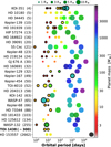 |
Fig. 15 Architectures of all 27 detected systems with minimum three planets and at least one inner small planet and one outer giant, including the TOI-1438 system assuming a planetary nature of signal d. The largest orbital period ratio between two adjacent planets in each system increases from top to bottom and is written in parentheses after the name of the host star. The sizes and colors of the circles indicate the radii and masses of the planets, respectively. Planets with transit measurements are outlined in black. All planets have RV measurements except for HD 73344 b, Kepler−167 b, c, and d, as well as the eight planets orbiting KOI-351. |
4.4 Formation of systems with small inner planets and outer giants
Both sub-Neptunes and Jovian planets are thought to mainly form via core accretion, where envelope accretion follows the accumulation of a solid core of ~10 M⊕ (Pollack et al. 1996). Variants are pebble accretion and planetesimal accretion, depending on the size of the dominant source of accreted solids. Modern versions of these models suggest that any correlation between close-in planets and outer gas giants arises because of the disc-wide dependence of planet formation arising from the global budget of solids in the disc. From planetesimal accretion models, Schlecker et al. (2021) found that co-existence of outer giant planets and smaller inner planets occurs preferentially for intermediate values of the quantity of solids: too little, and cores cannot grow large enough to begin gas accretion; too much, and multiple gas giants form, which typically destabilise the inner planets during instabilities (see also Mustill et al. 2017; Pu & Lai 2021). In models of pebble accretion, Bitsch & Izidoro (2023) found frequent co-existence of inner and outer planets if the envelope contraction is not overly efficient (i.e. avoiding growth of the inner sub-Neptunes to full gas giants). However, again, where multiple outer planets form, the instabilities among them can often reduce the multiplicity of the inner system (Bitsch et al. 2020). In the case of TOI-1438, the large separation between the dynamically cold inner sub-Neptunes and the outer giant may have helped preserve them from any instability (should one have occurred). The low (albeit non-zero) eccentricity of the outer planet might suggest a mild instability, with relatively little effect on the inner system (Pu & Lai 2021); this could indicate, for instance, the prior ejection of a relatively low-mass outer giant planet (Kokaia et al. 2020; Pu & Lai 2021).
5 Conclusions
In this paper, we present the detection and characterisation of the TOI-1438 system with two short-orbital period sub-Neptunes and a tentative Jupiter-like planet with an orbital period of  yr. If the latter is indeed a planet, it has a minimum mass of 2.1 ± 0.3 MJ. Overall, given the constraints on the orbital model parameters that make it possible to construct a global view of the dynamics, our stability analysis combined with the measured small TTV amplitudes and their predicted values in the parameter space favours an orbital model with nearly circular orbits of the inner subsystem. Long-period magnetic stellar activity seems to be present at some level, as indicated by several activity indicators. Thus, we cannot confirm the existence of planet d which remains a tentative discovery. More data are required to fully cover the entire orbital period of signal d and to resolve the long-period stellar activity signals. If it is confirmed as a triple-planet system, the architecture of TOI-1438 would exhibit one of the largest gaps between inner small planets and outer giant planets of all known systems so far. This particular aspect could point to further, undetected planets.
In our interior structure analysis, we considered both a water world structure with an iron core and a silicate-rich mantle, as well as a range of sub-Neptune structures with varying H/He mass fractions and mixed rock-water cores. TOI-1438 b and c present volatile-rich envelopes, which are a mixture of H/He and water. This is due to the fact that pure water envelopes require very high envelope mass fractions to explain their low densities (>50%). Planets b and c could contain up to 2.5% and 0.2% of H/He in mass, respectively. The compositions of their deep cores could not be constrained from mass and radius data alone due to degeneracies, which may range from cores constituted by rock and Fe to silicate melts with miscible water and other volatiles.
Acknowledgements
This paper includes data collected by the TESS mission. Funding for the TESS mission is provided by the NASA Explorer Program. We acknowledge the use of public TESS data from pipelines at the TESS Science Office and at the TESS Science Processing Operations Center. Funding for the TESS mission is provided by NASA’s Science Mission Directorate. Resources supporting this work were provided by the NASA High-End Computing (HEC) Program through the NASA Advanced Supercomputing (NAS) Division at Ames Research Center for the production of the SPOC data products. We also acknowledge the use of TESS High-Level Science Products (HLSP) produced by the Quick-Look Pipeline (QLP) at the TESS Science Office at MIT, which are publicly available from the Mikulski Archive for Space Telescopes (MAST) at the Space Telescope Science Institute (STScI). STScI is operated by the Association of Universities for Research in Astronomy, Inc., under NASA contract NAS 5-26555. This research has made use of the Exoplanet Follow-up Observation Program (ExoFOP; DOI: 10.26134/ExoFOP5) website, which is operated by the California Institute of Technology, under contract with the National Aeronautics and Space Administration under the Exoplanet Exploration Program. Some of the observations in this paper made use of the High-Resolution Imaging instrument ‘Alopeke and were obtained under Gemini LLP Proposal Number: GN/S-2021A-LP-105. ‘Alopeke was funded by the NASA Exoplanet Exploration Program and built at the NASA Ames Research Center by Steve B. Howell, Nic Scott, Elliott P. Horch, and Emmett Quigley. Alopeke was mounted on the Gemini North telescope of the international Gemini Observatory, a program of NSF’s OIR Lab, which is managed by the Association of Universities for Research in Astronomy (AURA) under a cooperative agreement with the National Science Foundation. on behalf of the Gemini partnership: the National Science Foundation (United States), National Research Council (Canada), Agencia Nacional de Investigación y Desarrollo (Chile), Ministerio de Ciencia, Tecnología e Innovación (Argentina), Ministério da Ciência, Tecnologia, Inovações e Comunicações (Brazil), and Korea Astronomy and Space Science Institute (Republic of Korea). This work has made use of SME package, which benefits from the continuing development work by J. Valenti and N. Piskunov and we gratefully acknowledge their continued support. We acknowledge fruitful discussions with Andreas Quirrenbach on stellar activity and the effect on RVs. C.M.P., M.F. and A.J.M. acknowledge the support of the Swedish National Space Agency (DNR 65/19, 177/19, and 2023-00146). C.M.P., E.K. and A.M. acknowledge the support of GENIE at Chalmers. Funding for the Stellar Astrophysics Centre is provided by The Danish National Research Foundation (Grant agreement no.: DNRF106). C.N.W. acknowledge support from the TESS mission via subaward s3449 from MIT. T.M. acknowledges support from the Spanish Ministry of Science and Innovation with the the proyecto plan nacional PLAtoSOnG (grant no. PID2023-146453NB-100). R.A.G., D.B.P., and L.B. acknowledge the support from the GOLF and PLATO Centre National D’Études Spatiales grants. S.M. and H.J.D. acknowledges support by the Spanish Ministry of Science and Innovation with the grants number PID2019-107061GB-C66 and PID2023-149439NB-C41, and through AEI under the Severo Ochoa Centres of Excellence Programme 2020-2023 (CEX2019-000920-S). K.G., D.J. and G.N. gratefully acknowledges the Centre of Informatics Tricity Academic Supercomputer and networK (CI TASK, Gdansk, Poland) for computing resources (grant no. PT01187). G.N. thanks for the research funding from the Ministry of Science and Higher Education programme the “Excellence Initiative – Research University” conducted at the Centre of Excellence in Astrophysics and Astrochemistry of the Nicolaus Copernicus University in Torun, Poland. G.M. acknowledges financial support from the Severo Ochoa grant CEX2021-001131-S and from the Ramón y Cajal grant RYC2022-037854-I funded by MCIN/AEI/1144 10.13039/501100011033 and FSE+. F.M. acknowledges the financial support from the Agencia Estatal de Investigación del Ministerio de Ciencia, Innovación y Universidades (MCIU/AEI) through grant PID2023-152906NA-I00. E.P. acknowledge financial support from the Agencia Estatal de Investigación of the Ministerio de Ciencia e Innovación MCIN/AEI/10.13039/501100011033 and the ERDF “A way of making Europe” through project PID2021-125627OB-C32, and from the Centre of Excellence “Severo Ochoa” award to the Instituto de Astrofisica de Canarias. R.L. acknowledges support for this work by NASA through the NASA Hubble Fellowship grant HST-HF2-51559.001-A awarded by the Space Telescope Science Institute, which is operated by the Association of Universities for Research in Astronomy, Inc., for NASA, under contract NAS5-26555. K.W.F.L. acknowledge support by European Union’s Horizon Europe Framework Programme under the Marie Skìodowska-Curie Actions grant agreement No. 101086149 (EXOWORLD). J.K. acknowledge support from the Swiss NCCR PlanetS and the Swiss National Science Foundation. This work has been carried out within the framework of the NCCR PlanetS supported by the Swiss National Science Foundation under grants 51NF40182901 and 51NF40205606. J.K. acknowledges support from the Swedish National Space Agency (SNSA; DNR 2020-00104) and of the Swiss National Science Foundation under grant number TMSGI2_211697. VVE. has been supported by UK’s Science & Technology Facilities Council through the STFC grants ST/W001136/1 and ST/S000216/1.
Data availability
Tables A.1 and A.3 are available at the CDS via https://cdsarc.cds.unistra.fr/viz-bin/cat/J/A+A/702/A69.
Appendix A Figures
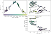 |
Fig. A.1 RVs vs time, differential line width (dLW) vs RVs, and dLW vs time. The models of planets b and c have been subtracted from the RVs. |
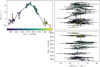 |
Fig. A.2 RVs vs time, RV chromatic index (CRX) vs RVs, and CRX vs time. The models of planets b and c have been subtracted from the RVs. |
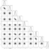 |
Fig. A.3 Corner plot of the posterior distributions of the joint transit and RV model of planet b. |
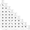 |
Fig. A.4 Corner plot of the posterior distributions of the joint transit and RV model of planet c. |
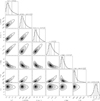 |
Fig. A.5 Corner plot of the posterior distributions of the RV model of signal d. |
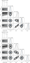 |
Fig. A.6 Corner plot of the posteriors of our MCMC retrieval of TOI-1438 b (top) and planet c (bottom) interior structures and compositions. |
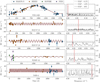 |
Fig. A.7 RV residuals for TOI-1438 and the four systems highlighted in Fig. 14 are shown in the plots to the left. The sinusoid shown in red in each of these is calculated from the most prominent peak highlighted in red in the associated GLS to the right. The false alarm probabilities are shown as horizontal lines, with values indicated in the legend. |
References
- Acuña, L., Deleuil, Magali, Mousis, Olivier, et al. 2021, A&A, 647, A53 [NASA ADS] [CrossRef] [EDP Sciences] [Google Scholar]
- Acuña, L., Kreidberg, L., Zhai, M., & Mollière, P. 2024, A&A, 688, A60 [NASA ADS] [CrossRef] [EDP Sciences] [Google Scholar]
- Acuña Aguirre, L. 2022, PhD thesis, université Aix-Marseille [Google Scholar]
- Aguichine, A., Mousis, O., Deleuil, M., & Marcq, E. 2021, ApJ, 914, 84 [NASA ADS] [CrossRef] [Google Scholar]
- Agúndez, M., Venot, O., Selsis, F., & Iro, N. 2014, ApJ, 781, 68 [Google Scholar]
- Aigrain, S., & Foreman-Mackey, D. 2023, ARA&A, 61, 329 [NASA ADS] [CrossRef] [Google Scholar]
- Aigrain, S., Llama, J., Ceillier, T., et al. 2015, MNRAS, 450, 3211 [Google Scholar]
- Allard, F., Homeier, D., & Freytag, B. 2012, Philos. Trans. Roy. Soc. Lond. A, 370, 2765 [NASA ADS] [Google Scholar]
- Angus, R., Morton, T. D., Foreman-Mackey, D., et al. 2019, AJ, 158, 173 [Google Scholar]
- Baliunas, S. L., Donahue, R. A., Soon, W. H., et al. 1995, ApJ, 438, 269 [Google Scholar]
- Baraffe, I., Chabrier, G., Barman, T. S., Allard, F., & Hauschildt, P. H. 2003, A&A, 402, 701 [NASA ADS] [CrossRef] [EDP Sciences] [Google Scholar]
- Baraffe, I., Chabrier, G., & Barman, T. 2008, A&A, 482, 315 [NASA ADS] [CrossRef] [EDP Sciences] [Google Scholar]
- Barkaoui, K., Sebastian, D., Zúñiga-Fernández, S., et al. 2025, A&A, 696, A44 [NASA ADS] [CrossRef] [EDP Sciences] [Google Scholar]
- Barnes, S. A. 2007, ApJ, 669, 1167 [Google Scholar]
- Barragán, O., Gandolfi, D., & Antoniciello, G. 2019, MNRAS, 482, 1017 [Google Scholar]
- Barragán, O., Aigrain, S., Rajpaul, V. M., & Zicher, N. 2022, MNRAS, 509, 866 [Google Scholar]
- Becker, J. C., & Adams, F. C. 2017, MNRAS, 468, 549 [NASA ADS] [CrossRef] [Google Scholar]
- Benneke, B., Roy, P.-A., Coulombe, L.-P., et al. 2024, arXiv e-prints, [arXiv:2403.03325] [Google Scholar]
- Bitsch, B., & Izidoro, A. 2023, A&A, 674, A178 [NASA ADS] [CrossRef] [EDP Sciences] [Google Scholar]
- Bitsch, B., Trifonov, T., & Izidoro, A. 2020, A&A, 643, A66 [EDP Sciences] [Google Scholar]
- Bonomo, A. S., Desidera, S., Benatti, S., et al. 2017, A&A, 602, A107 [NASA ADS] [CrossRef] [EDP Sciences] [Google Scholar]
- Bonomo, A. S., Dumusque, X., Massa, A., et al. 2023, A&A, 677, A33 [NASA ADS] [CrossRef] [EDP Sciences] [Google Scholar]
- Boro Saikia, S., Marvin, C. J., Jeffers, S. V., et al. 2018, A&A, 616, A108 [NASA ADS] [CrossRef] [EDP Sciences] [Google Scholar]
- Borucki, W. J., Koch, D., Basri, G., et al. 2010, Science, 327, 977 [Google Scholar]
- Bouchy, F., Pont, F., Melo, C., et al. 2005, A&A, 431, 1105 [NASA ADS] [CrossRef] [EDP Sciences] [Google Scholar]
- Boué, G., & Fabrycky, D. C. 2014, ApJ, 789, 111 [CrossRef] [Google Scholar]
- Bressan, A., Marigo, P., Girardi, L., et al. 2012, MNRAS, 427, 127 [NASA ADS] [CrossRef] [Google Scholar]
- Brinkman, C. L., Weiss, L. M., Huber, D., et al. 2024, arXiv e-prints, [arXiv:2410.00213] [Google Scholar]
- Brugger, B., Mousis, O., Deleuil, M., & Lunine, J. I. 2016, ApJ, 831, L16 [NASA ADS] [CrossRef] [Google Scholar]
- Brugger, B., Mousis, O., Deleuil, M., & Deschamps, F. 2017, ApJ, 850, 93 [NASA ADS] [CrossRef] [Google Scholar]
- Bruntt, H., Bedding, T. R., Quirion, P.-O., et al. 2010, MNRAS, 405, 1907 [NASA ADS] [Google Scholar]
- Bryan, M. L., & Lee, E. J. 2024, ApJ, 968, L25 [NASA ADS] [CrossRef] [Google Scholar]
- Bryan, M. L., Knutson, H. A., Lee, E. J., et al. 2019, AJ, 157, 52 [Google Scholar]
- Butler, R. P., & Marcy, G. W. 1996, ApJ, 464, L153 [NASA ADS] [CrossRef] [Google Scholar]
- Carmichael, T. W., Latham, D. W., & Vanderburg, A. M. 2019, AJ, 158, 38 [NASA ADS] [CrossRef] [Google Scholar]
- Castelli, F., & Kurucz, R. L. 2004, ArXiv e-prints [arXiv:astro-ph/0405087] [Google Scholar]
- Ceillier, T., Tayar, J., Mathur, S., et al. 2017, A&A, 605, A111 [NASA ADS] [CrossRef] [EDP Sciences] [Google Scholar]
- Chaturvedi, P., Chakraborty, A., Anandarao, B. G., Roy, A., & Mahadevan, S. 2016, MNRAS, 462, 554 [Google Scholar]
- Chaturvedi, P., Sharma, R., Chakraborty, A., Anandarao, B. G., & Prasad, N. J. S. S. V. 2018, AJ, 156, 27 [NASA ADS] [CrossRef] [Google Scholar]
- Chaturvedi, P., Bluhm, P., Nagel, E., et al. 2022, A&A, 666, A155 [NASA ADS] [CrossRef] [EDP Sciences] [Google Scholar]
- Chen, H., & Rogers, L. A. 2016, ApJ, 831, 180 [Google Scholar]
- Choi, J., Dotter, A., Conroy, C., et al. 2016, ApJ, 823, 102 [Google Scholar]
- Christian, D. J., Gibson, N. P., Simpson, E. K., et al. 2009, MNRAS, 392, 1585 [NASA ADS] [CrossRef] [Google Scholar]
- Ciardi, D. R., Beichman, C. A., Horch, E. P., & Howell, S. B. 2015, ApJ, 805, 16 [NASA ADS] [CrossRef] [Google Scholar]
- Cincotta, P. M., Giordano, C. M., & Simó, C. 2003, Physica D, 182, 151 [NASA ADS] [CrossRef] [Google Scholar]
- Claret, A. 2018, A&A, 618, A20 [NASA ADS] [CrossRef] [EDP Sciences] [Google Scholar]
- Claudi, R., Bruno, G., Fossati, L., et al. 2024, A&A, 682, A136 [NASA ADS] [CrossRef] [EDP Sciences] [Google Scholar]
- Collins, K. A., Kielkopf, J. F., Stassun, K. G., & Hessman, F. V. 2017, AJ, 153, 77 [Google Scholar]
- Cosentino, R., Lovis, C., Pepe, F., et al. 2012, Proc. SPIE, 8446, 84461V [Google Scholar]
- Cosentino, R., Lovis, C., Pepe, F., et al. 2014, SPIE Conf. Ser., 9147, 91478C [Google Scholar]
- Cresswell, P., & Nelson, R. P. 2022, MNRAS, 510, 620 [Google Scholar]
- da Silva, L., Girardi, L., Pasquini, L., et al. 2006, A&A, 458, 609 [NASA ADS] [CrossRef] [EDP Sciences] [Google Scholar]
- Deck, K. M., & Batygin, K. 2022, ApJ, 928, 118 [Google Scholar]
- Demory, B.-O., Ségransan, D., Forveille, T., et al. 2009, A&A, 505, 205 [NASA ADS] [CrossRef] [EDP Sciences] [Google Scholar]
- Díaz, R. F., Montagnier, G., Leconte, J., et al. 2014, A&A, 572, A109 [NASA ADS] [CrossRef] [EDP Sciences] [Google Scholar]
- Dorn, C., Khan, A., Heng, K., et al. 2015, A&A, 577, A83 [NASA ADS] [CrossRef] [EDP Sciences] [Google Scholar]
- Doyle, A. P., Davies, G. R., Smalley, B., Chaplin, W. J., & Elsworth, Y. 2014, MNRAS, 444, 3592 [Google Scholar]
- Feng, F., Butler, R. P., Vogt, S. S., et al. 2022, ApJS, 262, 21 [NASA ADS] [CrossRef] [Google Scholar]
- Foreman-Mackey, D. 2016, J. Open Source Softw., 1, 24 [Google Scholar]
- Foreman-Mackey, D., Hogg, D. W., Lang, D., & Goodman, J. 2013, PASP, 125, 306 [Google Scholar]
- Foreman-Mackey, D., Agol, E., Ambikasaran, S., & Angus, R. 2017, Astrophysics Source Code Library [record ascl:1709.008] [Google Scholar]
- Fossati, L., Erkaev, N. V., Lammer, H., et al. 2017, A&A, 598, A90 [NASA ADS] [CrossRef] [EDP Sciences] [Google Scholar]
- Fulton, B. J., & Petigura, E. A. 2018, AJ, 156, 264 [Google Scholar]
- Fulton, B. J., Petigura, E. A., Howard, A. W., et al. 2017, AJ, 154, 109 [Google Scholar]
- Furlan, E., & Howell, S. B. 2017, AJ, 154, 66 [NASA ADS] [CrossRef] [Google Scholar]
- García, R. A., Hekker, S., Stello, D., et al. 2011, MNRAS, 414, L6 [NASA ADS] [CrossRef] [Google Scholar]
- García, R. A., Mathur, S., Pires, S., et al. 2014, A&A, 568, A10 [Google Scholar]
- García, R. A., Palakkatharappil, D. B., Mathur, S., et al. 2024, in TESS Science Conference III, 32 [Google Scholar]
- Gillen, E., Hillenbrand, L. A., David, T. J., et al. 2017, ApJ, 849, 11 [Google Scholar]
- Gozdziewski, K., Bois, E., Maciejewski, A. J., & Kiseleva-Eggleton, L. 2001, A&A, 378, 569 [NASA ADS] [CrossRef] [EDP Sciences] [Google Scholar]
- Grieves, N., Bouchy, F., Lendl, M., et al. 2021, A&A, 652, A127 [NASA ADS] [CrossRef] [EDP Sciences] [Google Scholar]
- Guerrero, N. M., Seager, S., Huang, C. X., et al. 2021, ApJS, 254, 39 [NASA ADS] [CrossRef] [Google Scholar]
- Gustafsson, B., Edvardsson, B., Eriksson, K., et al. 2008, A&A, 486, 951 [NASA ADS] [CrossRef] [EDP Sciences] [Google Scholar]
- Hadden, S., & Payne, M. J. 2020, AJ, 160, 106 [NASA ADS] [CrossRef] [Google Scholar]
- Handberg, R., & Lund, M. N. 2014, MNRAS, 445, 2698 [Google Scholar]
- Hartman, J. D., Bakos, G. Á., Sato, B., et al. 2011, ApJ, 726, 52 [NASA ADS] [CrossRef] [Google Scholar]
- He, M. Y., & Weiss, L. M. 2023, AJ, 166, 36 [NASA ADS] [CrossRef] [Google Scholar]
- Hekker, S., Reffert, S., Quirrenbach, A., et al. 2006, A&A, 454, 943 [NASA ADS] [CrossRef] [EDP Sciences] [Google Scholar]
- Holmberg, M., & Madhusudhan, N. 2024, A&A, 683, L2 [NASA ADS] [CrossRef] [EDP Sciences] [Google Scholar]
- Howard, A. W., Johnson, J. A., Marcy, G. W., et al. 2010, ApJ, 721, 1467 [Google Scholar]
- Howard, A. W., Marcy, G. W., Bryson, S. T., et al. 2012, ApJS, 201, 15 [Google Scholar]
- Howell, S. B., & Furlan, E. 2022, Front. Astron. Space Sci., 9, 871163 [NASA ADS] [CrossRef] [Google Scholar]
- Howell, S. B., Everett, M. E., Sherry, W., Horch, E., & Ciardi, D. R. 2011, AJ, 142, 19 [Google Scholar]
- Howell, S. B., Sobeck, C., Haas, M., et al. 2014, PASP, 126, 398 [Google Scholar]
- Howell, S. B., Scott, N. J., Matson, R. A., et al. 2021, Front. Astron. Space Sci., 8, 10 [NASA ADS] [Google Scholar]
- Huang, C. X., Vanderburg, A., Pál, A., et al. 2020a, RNAAS, 4, 204 [Google Scholar]
- Huang, C. X., Vanderburg, A., Pál, A., et al. 2020b, RNAAS, 4, 206 [NASA ADS] [Google Scholar]
- Hunter, A. A., Macgregor, A. B., Szabo, T. O., Wellington, C. A., & Bellgard, M. I. 2012, Source Code Biol. Med., 7, 1 [Google Scholar]
- Husser, T. O., Wende-von Berg, S., Dreizler, S., et al. 2013, A&A, 553, A6 [NASA ADS] [CrossRef] [EDP Sciences] [Google Scholar]
- Jenkins, J. M. 2002, ApJ, 575, 493 [Google Scholar]
- Jenkins, J. M., Chandrasekaran, H., McCauliff, S. D., et al. 2010, SPIE Conf. Ser., 7740, 77400D [Google Scholar]
- Jenkins, J. M., Twicken, J. D., McCauliff, S., et al. 2016, SPIE Conf. Ser., 9913, 99133E [Google Scholar]
- Jenkins, J. M., Tenenbaum, P., Seader, S., et al. 2020, Kepler Data Processing Handbook: Transiting Planet Search, Kepler Science Document KSCI-19081-003, 9, ed. J. M. Jenkins. [Google Scholar]
- Kempton, E. M. R., Bean, J. L., Louie, D. R., et al. 2018, PASP, 130, 114401 [Google Scholar]
- Kipping, D. M. 2013, MNRAS, 434, L51 [Google Scholar]
- Kite, E. S., Fegley, Jr., B., Schaefer, L., & Ford, E. B. 2019, ApJ, 887, L33 [NASA ADS] [CrossRef] [Google Scholar]
- Knutson, H. A., Fulton, B. J., Montet, B. T., et al. 2014, ApJ, 785, 126 [NASA ADS] [CrossRef] [Google Scholar]
- Kokaia, G., Davies, M. B., & Mustill, A. J. 2020, MNRAS, 492, 352 [Google Scholar]
- Kovács, G., Bakos, G. Á., Hartman, J. D., et al. 2010, ApJ, 724, 866 [CrossRef] [Google Scholar]
- Kreidberg, L. 2015, PASP, 127, 1161 [Google Scholar]
- Kuerster, M., Schmitt, J. H. M. M., Cutispoto, G., & Dennerl, K. 1997, A&A, 320, 831 [Google Scholar]
- Kunimoto, M., Tey, E., Fong, W., et al. 2022, RNAAS, 6, 236 [NASA ADS] [Google Scholar]
- Kunimoto, M., Vanderburg, A., Huang, C. X., et al. 2023, AJ, 166, 7 [NASA ADS] [CrossRef] [Google Scholar]
- Kurucz, R. L. 1993, VizieR Online Data Catalog: VI/39 [Google Scholar]
- Lai, D., & Pu, B. 2017, AJ, 153, 42 [Google Scholar]
- Leleu, A., Delisle, J.-B., Burn, R., et al. 2024, A&A, 687, L1 [NASA ADS] [CrossRef] [EDP Sciences] [Google Scholar]
- Li, J., Tenenbaum, P., Twicken, J. D., et al. 2019, PASP, 131, 024506 [NASA ADS] [CrossRef] [Google Scholar]
- Liu, Z., & Ni, D. 2023, A&A, 674, A137 [NASA ADS] [CrossRef] [EDP Sciences] [Google Scholar]
- Livesey, J. R., & Becker, J. 2025, ApJ, 979, 202 [Google Scholar]
- Luo, H., Dorn, C., & Deng, J. 2024, Nat. Astron., 8, 1399 [Google Scholar]
- Malavolta, L., Nascimbeni, V., Piotto, G., et al. 2016, A&A, 588, A118 [NASA ADS] [CrossRef] [EDP Sciences] [Google Scholar]
- Malavolta, L., Mayo, A. W., Louden, T., et al. 2018, AJ, 155, 107 [NASA ADS] [CrossRef] [Google Scholar]
- Mamajek, E. E., & Hillenbrand, L. A. 2008, ApJ, 687, 1264 [Google Scholar]
- Mandushev, G., O’Donovan, F. T., Charbonneau, D., et al. 2007, ApJ, 667, L195 [NASA ADS] [CrossRef] [Google Scholar]
- Marcy, G. W., Isaacson, H., Howard, A. W., et al. 2014, ApJS, 210, 20 [NASA ADS] [CrossRef] [Google Scholar]
- Masuda, K., & Winn, J. N. 2020, AJ, 159, 81 [NASA ADS] [CrossRef] [Google Scholar]
- Mathur, S., García, R. A., Régulo, C., et al. 2010, A&A, 511, A46 [NASA ADS] [CrossRef] [EDP Sciences] [Google Scholar]
- Mathur, S., Claytor, Z. R., Santos, Â. R. G., et al. 2023, ApJ, 952, 131 [NASA ADS] [CrossRef] [Google Scholar]
- Matson, R. A., Howell, S. B., Horch, E. P., & Everett, M. E. 2018, AJ, 156, 31 [NASA ADS] [CrossRef] [Google Scholar]
- Mayor, M., Pepe, F., Queloz, D., et al. 2003, The Messenger, 114, 20 [NASA ADS] [Google Scholar]
- Mazevet, S., Licari, A., Chabrier, G., & Potekhin, A. Y. 2019, A&A, 621, A128 [NASA ADS] [CrossRef] [EDP Sciences] [Google Scholar]
- McQuillan, A., Aigrain, S., & Mazeh, T. 2013, MNRAS, 432, 1203 [Google Scholar]
- Millholland, S., Wang, S., & Laughlin, G. 2017, ApJ, 849, L33 [NASA ADS] [CrossRef] [Google Scholar]
- Mills, S. M., Fabrycky, D. C., Migaszewski, C., & Ford, E. B. 2023, AJ, 165, 72 [CrossRef] [Google Scholar]
- Morris, R. L., Twicken, J. D., Smith, J. C., et al. 2020, Kepler Data Processing Handbook: Photometric Analysis, Kepler Science Document KSCI-19081-003, 6. Ed. J. M. Jenkins [Google Scholar]
- Müller, S., Baron, J., Helled, R., Bouchy, F., & Parc, L. 2024, A&A, 686, A296 [NASA ADS] [CrossRef] [EDP Sciences] [Google Scholar]
- Muresan, A., Persson, C. M., & Fridlund, M. 2024, A&A, 692, A122 [NASA ADS] [CrossRef] [EDP Sciences] [Google Scholar]
- Murray, C. D., & Correia, A. C. M. 2010, in Exoplanets, ed. S. Seager, 15 [Google Scholar]
- Mustill, A. J., Davies, M. B., & Johansen, A. 2017, MNRAS, 468, 3000 [Google Scholar]
- Otegi, J. F., Dorn, C., Helled, R., et al. 2020, A&A, 640, A135 [NASA ADS] [CrossRef] [EDP Sciences] [Google Scholar]
- Palakkatharappil, D. B., Gilles, M., García, R. A., et al. 2024, in 8th TESS/15th [Google Scholar]
- Kepler Asteroseismic Science Consortium Workshop, 93 [Google Scholar]
- Panichi, F., Gozdziewski, K., & Turchetti, G. 2017, MNRAS, 468, 469 [Google Scholar]
- Papaloizou, J. C. B., & Szuszkiewicz, E. 2005, MNRAS, 363, 153 [Google Scholar]
- Persson, C. M., Fridlund, M., Barragán, O., et al. 2018, A&A, 618, A33 [NASA ADS] [CrossRef] [EDP Sciences] [Google Scholar]
- Piaulet-Ghorayeb, C., Benneke, B., Radica, M., et al. 2024, ApJ, 974, L10 [NASA ADS] [CrossRef] [Google Scholar]
- Pires, S., Mathur, S., García, R. A., et al. 2015, A&A, 574, A18 [NASA ADS] [CrossRef] [EDP Sciences] [Google Scholar]
- Piskunov, N., & Valenti, J. A. 2017, A&A, 597, A16 [NASA ADS] [CrossRef] [EDP Sciences] [Google Scholar]
- Plotnykov, M., & Valencia, D. 2020, MNRAS, 499, 932 [CrossRef] [Google Scholar]
- Polanski, A. S., Lubin, J., Beard, C., et al. 2024, ApJS, 272, 32 [NASA ADS] [CrossRef] [Google Scholar]
- Pollack, J. B., Hubickyj, O., Bodenheimer, P., et al. 1996, Icarus, 124, 62 [NASA ADS] [CrossRef] [Google Scholar]
- Pont, F., Bouchy, F., Melo, C., et al. 2005, A&A, 438, 1123 [NASA ADS] [CrossRef] [EDP Sciences] [Google Scholar]
- Pont, F., Moutou, C., Bouchy, F., et al. 2006, A&A, 447, 1035 [NASA ADS] [CrossRef] [EDP Sciences] [Google Scholar]
- Poon, S. T. S., & Nelson, R. P. 2020, MNRAS, 498, 5166 [NASA ADS] [CrossRef] [Google Scholar]
- Pu, B., & Lai, D. 2021, MNRAS, 508, 597 [CrossRef] [Google Scholar]
- Rajpaul, V., Aigrain, S., Osborne, M. A., Reece, S., & Roberts, S. 2015, MNRAS, 452, 2269 [Google Scholar]
- Rein, H., & Liu, S. F. 2012, A&A, 537, A128 [NASA ADS] [CrossRef] [EDP Sciences] [Google Scholar]
- Rein, H., & Spiegel, D. S. 2015, MNRAS, 446, 1424 [Google Scholar]
- Ribas, I. 2003, A&A, 398, 239 [NASA ADS] [CrossRef] [EDP Sciences] [Google Scholar]
- Ricker, G. R., Winn, J. N., Vanderspek, R., et al. 2015, J. Astron. Telesc. Instrum. Syst., 1, 014003 [Google Scholar]
- Rodet, L., & Lai, D. 2021, MNRAS, 502, 3746 [Google Scholar]
- Ryabchikova, T., Piskunov, N., Kurucz, R. L., et al. 2015, Phys. Scr, 90, 054005 [Google Scholar]
- Salabert, D., García, R. A., Beck, P. G., et al. 2016, A&A, 596, A31 [NASA ADS] [CrossRef] [EDP Sciences] [Google Scholar]
- Santos, A. R. G., García, R. A., Mathur, S., et al. 2019, ApJS, 244, 21 [Google Scholar]
- Santos, A. R. G., Breton, S. N., Mathur, S., & García, R. A. 2021, ApJS, 255, 17 [NASA ADS] [CrossRef] [Google Scholar]
- Schlecker, M., Mordasini, C., Emsenhuber, A., et al. 2021, A&A, 656, A71 [NASA ADS] [CrossRef] [EDP Sciences] [Google Scholar]
- Schlegel, D. J., Finkbeiner, D. P., & Davis, M. 1998, ApJ, 500, 525 [Google Scholar]
- Schlichting, H. E., & Young, E. D. 2022, PSJ, 3, 127 [NASA ADS] [Google Scholar]
- Schulze, J. G., Wang, J., Johnson, J. A., et al. 2021, PSJ, 2, 113 [Google Scholar]
- Scott, N. J., Howell, S. B., Gnilka, C. L., et al. 2021, Front. Astron. Space Sci., 8, 138 [NASA ADS] [CrossRef] [Google Scholar]
- Seager, S., & Mallén-Ornelas, G. 2003, ApJ, 585, 1038 [Google Scholar]
- Serrano, L. M., Gandolfi, D., Mustill, A. J., et al. 2022, Nat. Astron., 6, 736 [NASA ADS] [CrossRef] [Google Scholar]
- Shporer, A., Zhou, G., Vanderburg, A., et al. 2017, ApJ, 847, L18 [Google Scholar]
- Smith, J. C., Stumpe, M. C., Van Cleve, J. E., et al. 2012, PASP, 124, 1000 [Google Scholar]
- Steffen, J. H., Fabrycky, D. C., Agol, E., et al. 2013, MNRAS, 428, 1077 [NASA ADS] [CrossRef] [Google Scholar]
- Stevenson, A. T., Haswell, C. A., Faria, J. P., et al. 2025, MNRAS, 539, 727 [Google Scholar]
- Stumpe, M. C., Smith, J. C., Van Cleve, J. E., et al. 2012, PASP, 124, 985 [Google Scholar]
- Stumpe, M. C., Smith, J. C., Catanzarite, J. H., et al. 2014, PASP, 126, 100 [Google Scholar]
- Tal-Or, L., Mazeh, T., Alonso, R., et al. 2013, A&A, 553, A30 [NASA ADS] [CrossRef] [EDP Sciences] [Google Scholar]
- Torrence, C., & Compo, G. P. 1998, Bull. Am. Meteorol. Soc., 79, 61 [Google Scholar]
- Torres, G., Andersen, J., & Giménez, A. 2010, A&A Rev., 18, 67 [Google Scholar]
- Twicken, J. D., Clarke, B. D., Bryson, S. T., et al. 2010, SPIE Conf. Ser., 7740, 774023 [NASA ADS] [Google Scholar]
- Twicken, J. D., Catanzarite, J. H., Clarke, B. D., et al. 2018, PASP, 130, 064502 [Google Scholar]
- Uehara, S., Kawahara, H., Masuda, K., Yamada, S., & Aizawa, M. 2016, ApJ, 822, 2 [NASA ADS] [CrossRef] [Google Scholar]
- Valenti, J. A., & Piskunov, N. 1996, A&AS, 118, 595 [NASA ADS] [CrossRef] [EDP Sciences] [Google Scholar]
- Van Zandt, J., & Petigura, E. A. 2024, AJ, 168, 268 [Google Scholar]
- Van Zandt, J., Petigura, E. A., Lubin, J., et al. 2025, arXiv e-prints, [arXiv:2581.86342] [Google Scholar]
- Vazan, A., Sari, R., & Kessel, R. 2022, ApJ, 926, 150 [NASA ADS] [CrossRef] [Google Scholar]
- Vines, J. I., & Jenkins, J. S. 2022, MNRAS, 513, 2719 [NASA ADS] [CrossRef] [Google Scholar]
- Vogt, S. S., Allen, S. L., Bigelow, B. C., et al. 1994, SPIE Conf. Ser., 2198, 362 [NASA ADS] [Google Scholar]
- von Boetticher, A., Triaud, A. H. M. J., Queloz, D., et al. 2017, A&A, 604, L6 [NASA ADS] [CrossRef] [EDP Sciences] [Google Scholar]
- Vowell, N., Rodriguez, J. E., Latham, D. W., et al. 2025, arXiv e-prints, [arXiv:2581.89795] [Google Scholar]
- Weiss, L., Isaacson, H., Marcy, G., et al. 2023, in American Astronomical Society Meeting Abstracts, 241, 316.03 [Google Scholar]
- Weiss, L. M., Marcy, G. W., Petigura, E. A., et al. 2018, AJ, 155, 48 [Google Scholar]
- Wilson, O. C. 1978, ApJ, 226, 379 [Google Scholar]
- Xu, W., & Fabrycky, D. C. 2019, ApJ, 875, 67 [NASA ADS] [CrossRef] [Google Scholar]
- Yee, S. W., Petigura, E. A., & von Braun, K. 2017, ApJ, 836, 77 [Google Scholar]
- Zakamska, N. L., Pan, M., & Ford, E. B. 2011, MNRAS, 410, 1895 [NASA ADS] [Google Scholar]
- Zechmeister, M., & Kürster, M. 2009, A&A, 496, 577 [CrossRef] [EDP Sciences] [Google Scholar]
- Zechmeister, M., Reiners, A., Amado, P. J., et al. 2018, A&A, 609, A12 [NASA ADS] [CrossRef] [EDP Sciences] [Google Scholar]
- Zeng, L., Jacobsen, S. B., Sasselov, D. D., et al. 2019, PNAS, 116, 9723 [Google Scholar]
- Zhou, G., Bayliss, D., Hartman, J. D., et al. 2014, MNRAS, 437, 2831 [Google Scholar]
- Zhu, W. 2024, Res. Astron. Astrophys., 24, 045013 [CrossRef] [Google Scholar]
KESPRINT is an international consortium devoted to the characterisation and research of exoplanets discovered with space-based missions, https://kesprint.science
Observing programs: CAT19A_162 (15 spectra), CAT21A_119 (8), CAT22A_111 (23) – PI: Nowak; ITP19_1 (2) – PI: Pallé; A41TAC_49 (5) – PI: Gandolfi; CAT20B_80 (1) – PI: Casasayas; CAT23A_52 (16), CAT23B_74 (10), CAT24B_20 (5) – PI: Carleo.
All Tables
Comparison of stellar mass and radius of TOI-1438 derived by different methods compared to values of a typical K0V star.
Summary models of planets b and c with free (model i) and fixed eccentricities (model ii).
Best fit compositional parameters, planetary masses, and equilibrium temperatures derived from our MCMC interior structure analysis.
All Figures
|
Fig. 1 Final results of the Gemini North speckle imaging of TOI-1438. The blue and red curves show the 5 σ contrast curves in 562 nm and 832 nm filters, respectively, as a function of the angular separation out to 1.2". The inset shows the reconstructed 832 nm image with a 1" scale bar. TOI-1438 was found to have no close companions from the diffraction limit out to 1.2" and within the magnitude contrast levels achieved. |
| In the text | |
|
Fig. 2 SED of TOI-1438 and the model with highest probability (Castelli & Kurucz 2004) are plotted together with the synthetic photometry (magenta diamonds) and the observed photometry (blue points). The vertical error bars outlines the 1 σ uncertainties and the horizontal bars the effective width of the passbands. The residuals of the fit (normalised to the errors of the photometry) are shown in the lower panel. |
| In the text | |
|
Fig. 3 GLS periodogram of the HARPS-N and HIRES RV data. The GLS of the raw RVs are shown in the top panel and the below panels have the best-fitting models subtracted for a given planet or signal d, as described in Sect. 3.4. From right to left, the orange, red, and blue vertical lines denotes the orbital periods of planets b and c, and signal d, respectively. |
| In the text | |
|
Fig. 4 GLS periodogram of HARPS-N data with activity indicators from DRS and Serval as indicated in the legends. The preliminary stellar rotation period of 23 days and Earth’s orbital period of 365 days are marked with red and green vertical dashed lines, respectively, and signal d with a blue vertical thick line. |
| In the text | |
|
Fig. 5 Emission in the line cores of the Ca II H & K absorption lines in the co-added HARPS spectrum of TOI-1438. |
| In the text | |
|
Fig. 6 TESS photometry of TOI-1438. Top: the de-trended TESS time series colour-coded according to sector; from black in Sector 14 to light copper in Sector 81. The data from Sector 74 is under the red cross and was excluded from the analysis. In total, there are 150 and 79 transits of planets b and c, respectively (excluding Sector 74). Middle: the phasefolded light curves for planets b (left) and c (right). The unbinned data are shown as small, grey markers, and the larger markers are ~10 min binned data colour-coded as in the top panel. The best-fitting models are shown as the white lines. Bottom: residuals from subtracting the best-fitting models from the data. |
| In the text | |
|
Fig.7 RVs of TOI-1438. Top: the HARPS-N (blue) and HIRES (orange) RV time series with the best-fitting three Keplerian model in grey with residuals shown in the panel below. Lower: the phasefolded RV curves for planet b (left) and c (middle) as well as signal d (right). The best-fitting models are shown as the grey lines with the shaded area denoting the 1 and 2 σ intervals in the K-amplitude. Residuals are given below. |
| In the text | |
|
Fig. 8 Dynamical maps of the eccentricities of the two inner planets (eb, ec) and fixed values of the argument of pericentre of TOI-1438 b(∆ϖ = ωc − ωb). The black filled circle with a white rim shows the location of the solution obtained by modelling with the eccentricities set as free parameters. Small values of the fast indicator log REM characterises regular (long-term stable) solutions, which are marked with black and dark blue colour. Chaotic solutions are marked with brighter colours, up to yellow. The black line represents the so-called collision curve of orbits, defined by the condition: αb(1 + eb) = ac(1 − ec). The resolution of each plot is 301 × 301 points. Triangles marked 1-3 correspond to the solutions shown in Fig. 9. Also, the labelled grey contours refer to the TTV amplitudes shown in Fig. 10 (details in Section 3.5). |
| In the text | |
|
Fig. 9 Temporal evolution of eccentricities for the representative solution selected in the dynamical maps shown in Fig. 8. The eccentricity of TOI-1438 b and TOI-1438 c are marked in blue and orange, respectively. |
| In the text | |
|
Fig. 10 TTV amplitudes in the (eb, ec)-plane and fixed initial values of the argument of pericentre TOI-1438 b (∆ϖ = ωc − ωb), computed for the RV data time span. The black filled circle with a white rim shows the location of the solution obtained with a model where the eccentricities are set as free parameters. |
| In the text | |
|
Fig. 11 TTV measurements based on the TESS photometric data (and spanning all but two sectors) skipped due to excessive noise. |
| In the text | |
|
Fig. 12 Density vs radius diagram of the 230 planets in 159 multiplanet systems with ≥2 planets from the NASA exoplanet archive with uncertainties better than 21% and 7% in mass and radius, respectively, color-coded with instellation. The planets plotted in grey are single planet systems. The masses are derived from RV measurements (181 planets) or from TTVs (49 planets outlined in dark grey), and the radii from transit photometry. Solar System planets are marked with brown squares. Low-mass stars are marked with yellow star symbols. TOI-1438 b and c are marked with red star symbols and fall within the diagonal strip of (sub-)Neptunes which displays decreasing density with increasing radius. The interior models for low mass-planets are from Zeng et al. (2019), and the solid black line shows the interior model of H/He dominated giant objects with Z = 0.02, age = 5 Gyr, and no irradiation (Baraffe et al. 2003, 2008). |
| In the text | |
|
Fig. 13 Mass-radius relationships for TOI-1438 b (left panel) and c (right panel). The GASTLI interior structure models are flexible enough to incorporate an inner deep layer of equal parts rock and water (50% each), along with a H/He envelope containing variable metal content. We adopt an intrinsic temperature Tint = 50 K (see text) across all models. The observed masses and radii of TOI-1438 b and c support multiple possible interior configurations, from planets with Fe-rich cores and isolated irradiated hydrospheres to those with mixed rock-water interiors covered by envelopes of varying H/He and metal proportions. |
| In the text | |
|
Fig. 14 RV jitter (σ1) as derived in Bonomo et al. (2017) as a function of log R′HK activity index calculated in Claudi et al. (2024) for exoplanet host stars with M⋆ < 1.1 M⊙. Light-grey error bars denote systems with a baseline shorter than 1 yr, grey error bars are systems with a baseline 1-2 yr, and black error bars are systems with baselines >2 yr. The error bars with arrows are upper limits on the RV jitter. The markers are colour coded with the stellar Teff. TOI-1438 is marked with a square. The marked systems HAT-P-15, HAT-P-19, TrES-4, and WASP-10 are discussed in Sect. 4.3. Adapted from Fig. 3 in Hekker et al. (2006). |
| In the text | |
|
Fig. 15 Architectures of all 27 detected systems with minimum three planets and at least one inner small planet and one outer giant, including the TOI-1438 system assuming a planetary nature of signal d. The largest orbital period ratio between two adjacent planets in each system increases from top to bottom and is written in parentheses after the name of the host star. The sizes and colors of the circles indicate the radii and masses of the planets, respectively. Planets with transit measurements are outlined in black. All planets have RV measurements except for HD 73344 b, Kepler−167 b, c, and d, as well as the eight planets orbiting KOI-351. |
| In the text | |
|
Fig. A.1 RVs vs time, differential line width (dLW) vs RVs, and dLW vs time. The models of planets b and c have been subtracted from the RVs. |
| In the text | |
|
Fig. A.2 RVs vs time, RV chromatic index (CRX) vs RVs, and CRX vs time. The models of planets b and c have been subtracted from the RVs. |
| In the text | |
|
Fig. A.3 Corner plot of the posterior distributions of the joint transit and RV model of planet b. |
| In the text | |
|
Fig. A.4 Corner plot of the posterior distributions of the joint transit and RV model of planet c. |
| In the text | |
|
Fig. A.5 Corner plot of the posterior distributions of the RV model of signal d. |
| In the text | |
|
Fig. A.6 Corner plot of the posteriors of our MCMC retrieval of TOI-1438 b (top) and planet c (bottom) interior structures and compositions. |
| In the text | |
|
Fig. A.7 RV residuals for TOI-1438 and the four systems highlighted in Fig. 14 are shown in the plots to the left. The sinusoid shown in red in each of these is calculated from the most prominent peak highlighted in red in the associated GLS to the right. The false alarm probabilities are shown as horizontal lines, with values indicated in the legend. |
| In the text | |
Current usage metrics show cumulative count of Article Views (full-text article views including HTML views, PDF and ePub downloads, according to the available data) and Abstracts Views on Vision4Press platform.
Data correspond to usage on the plateform after 2015. The current usage metrics is available 48-96 hours after online publication and is updated daily on week days.
Initial download of the metrics may take a while.