| Issue |
A&A
Volume 702, October 2025
|
|
|---|---|---|
| Article Number | A109 | |
| Number of page(s) | 12 | |
| Section | Cosmology (including clusters of galaxies) | |
| DOI | https://doi.org/10.1051/0004-6361/202555390 | |
| Published online | 14 October 2025 | |
Starlight from JWST: Implications for star formation and dark matter models
1
Keemilise ja Bioloogilise Füüsika Instituut, Rävala pst. 10, 10143 Tallinn, Estonia
2
Department of Cybernetics, Tallinn University of Technology, Akadeemia tee 21, 12618 Tallinn, Estonia
3
King’s College London, Strand, London, WC2R 2LS
United Kingdom
4
Theoretical Physics Department, CERN, Geneva, Switzerland
5
Dipartimento di Fisica e Astronomia, Università degli Studi di Padova, Via Marzolo 8, 35131 Padova, Italy
6
Istituto Nazionale di Fisica Nucleare, Sezione di Padova, Via Marzolo 8, 35131 Padova, Italy
⋆ Corresponding author: This email address is being protected from spambots. You need JavaScript enabled to view it.
Received:
5
May
2025
Accepted:
12
August
2025
Abstract
We compared the star formation rate in different dark matter (DM) models with UV luminosity data from JWST up to z ≃ 25 and legacy data from HST. We find that a transition from a Salpeter population to top-heavy Pop III stars is likely at z ≃ 10, and that beyond z = 10 − 15 the feedback from supernovae and active galactic nuclei is progressively reduced, so that at z ≃ 25 the production of stars is almost free from any feedback. We compared fuzzy and warm DM models that suppress small-scale structures with the CDM paradigm, and find that the fuzzy DM mass > 5.6 × 10⁻²² eV and the warm DM mass > 1.5 keV at a 95% CL. The fits of the star formation rate parametrisation do not depend strongly on the DM properties within the allowed range. We find no preference over CDM for enhanced matter perturbations associated with axion mini-clusters or primordial black holes. The scale of the enhancement of the power spectrum should be > 25 Mpc−1 at the 95% CL, excluding axion mini-clusters produced for ma < 6.6 × 10⁻¹⁷ eV or heavy primordial black holes that constitute a fraction fPBH > max[105 M⊙/mPBH, 10−4(mPBH/104 M⊙)−0.09] of DM.
Key words: cosmology: theory / dark matter
© The Authors 2025
 Open Access article, published by EDP Sciences, under the terms of the Creative Commons Attribution License (https://creativecommons.org/licenses/by/4.0), which permits unrestricted use, distribution, and reproduction in any medium, provided the original work is properly cited.
This article is published in open access under the Subscribe to Open model. This email address is being protected from spambots. You need JavaScript enabled to view it. to support open access publication.
1. Introduction
An important target for James Webb Space Telescope (JWST) observations is to measure the UV luminosity function at high z (Naidu et al. 2022b; Castellano 2023; Donnan et al. 2023; Morishita & Stiavelli 2023; Bouwens et al. 2023; Pérez-González et al. 2023; Harikane et al. 2023, 2024; Pérez-González et al. 2025; Castellano et al. 2025). These observations complement the more precise lower-z observations from the Hubble Space Telescope (HST) (McLeod et al. 2016; Oesch et al. 2018; Bouwens et al. 2021; Finkelstein et al. 2022; Leethochawalit et al. 2023; Bagley et al. 2024). The high-z observations serve as a probe of galaxy dynamics and the star formation rate (SFR) at early epochs of the universe, constraining the abundance and masses of the conjectured first-generation Pop III stars (Maiolino 2024; Vanzella et al. 2023; Ventura et al. 2024; Fujimoto et al. 2025). The frontier of UV luminosity function measurements has been pushed back to unprecedented early times with recent measurements at z ∼ 25, opening a window on the epoch before reionisation took place (Pérez-González et al. 2025; Castellano et al. 2025).
The number density of Pop III stars depends on the abundance of early galaxies. This depends in turn on the nature of dark matter (DM) since galaxies populate DM halos. The UV luminosity function is therefore a valuable source of insights into DM models (Sabti et al. 2022b; Hütsi et al. 2023; Parashari & Laha 2023; Liu et al. 2024; Winch et al. 2024; Sipple et al. 2025). As the redshift increases, the halo mass function (HMF) becomes more sensitive to the physical properties of DM since fewer halos are built via hierarchical growth and the imprints from the physics before the CMB are more noticeable.
Our understanding of structure formation and the star formation process in models of DM with suppressed small-scale structure formation at high z ≳ 10, such as fuzzy dark matter (FDM) and warm dark matter (WDM), or in models with an enhanced matter power spectrum is very limited. Therefore, the very high redshift abundance and distribution of Pop III stars, made of pristine gas from the Big Bang, are topics of hot debate. The roles of external radiation, internal fragmentation of the gas clouds and the dynamics that form the stars are highly uncertain, so the environments where these first stars were born and their mass function are as yet unknown (see Klessen & Glover 2023 for a review). The UV luminosity function measured with JWST has proven to be higher than anticipated, even when considering only the galaxies that are spectroscopically confirmed (Harikane et al. 2024). This suggests either that the feedback mechanisms preventing star formation were less restrictive (Susa & Umemura 2004; Dekel et al. 2023; Fukushima & Yajima 2021) or that the Pop III stars were very top-heavy, and therefore more luminous (Hirano et al. 2015; Steinhardt et al. 2023; Hirano et al. 2014; Chakraborty & Choudhury 2024). This tension has been exacerbated by the measurements of starlight at z ∼ 25, which are higher than the predictions from many semi-analytical models in the literature (Pérez-González et al. 2025).
The objectives of this work are to parametrise the essential physics of high-z star formation and to understand the features necessary to reproduce the UV luminosity function back to z ∼ 25 in different DM models. We took into account possible degeneracies and features of modified DM models, feedback, and changes in the stellar population. To this end, we connected the HMF obtained using the excursion set formalism (Bond et al. 1991), with the early Universe microphysics of DM, and combined this with a phenomenological parametrisation of star formation. We also discuss the effects of gravitational lensing and dust attenuation, neither of which seems to be very significant for the interpretation of the z > 15 UV data.
To extrapolate the results of DM simulations from low to high z and to obtain reliable bounds, we improved on existing techniques in the literature in two key aspects. First, we derived a new estimate of the DM halo growth rate that accounts for the ellipsoidal collapse correction, and used it consistently for different DM models. To this end, we recomputed the first-crossing probability distributions of the paths with a moving barrier and found a better fit than that originally proposed by Sheth et al. (2001). The conditional mass function in the Sheth-Tormen approach is divergent for very small steps, as has been pointed out by Jiang & van den Bosch (2014) and Zhang et al. (2008). Our fit is divergence-free and reproduces analytical estimations of Zhang et al. (2008). Second, we provide new values for the parameters the smooth-k window function that, unlike those proposed in Leo et al. (2018), consistently match the CDMprediction.
We find that, under the assumption that the star formation rate (SFR) is proportional to the halo growth rate, the observations of the UV luminosity function up to high z indicate two interesting effects that change the luminosity function. First, at z > 10, the stars need to be more luminous and/or the SFR needs to be higher. This transition is relatively sharp and might be caused by a top-heavy Pop III-dominated star population. We find that the evidence for this effect is above the 95% CL. In addition, the SFR needs to be further enhanced at z > 15. This can be achieved by reducing the feedback from supernovae (SNe) and active galactic nuclei (AGNs) on the SFR. We find that to explain the z > 15 observations, this feedback needs to be significantly reduced to match the UV luminosity function, and at z ≃ 25 the production of stars should be almost free from feedback effects. In agreement with Yung et al. (2025), with these changes in the stellar population and feedback effects, we find that the JWST data can be explained within the CDM model.
An important focus of this work is whether different DM scenarios require different star formation physics to fit the high-redshift data. Interestingly, we find very little sensitivity to DM properties that differ from CDM, with only a small change in star formation rates favoured for WDM, and no change for FDM.
When marginalizing over the SFR parametrisation, we find a lower bound of mFDM > 5.6 × 10⁻²²eV for the case of FDM and mWDM > 1.5 keV for the case of WDM. The new JWST data push the observations to much earlier galaxies, and yet they are still not precise enough to put much stronger bounds than the HST data, as also found in Winch et al. (2024). We also find that enhanced small-scale matter perturbations are not preferred over changes in the star formation, due to the presence of Pop III stars and changes in the feedback in the pre-reionisation era. We are able to put bounds on the scale of white-noise enhanced perturbations at kc > 25 Mpc−1, excluding, for example, the possibility of axion mini-clusters produced for ma < 6.6 × 10⁻¹⁷ eV or heavy primordial black holes (PBHs) that constitute the fraction fPBH > max[105 M⊙/mPBH, 10−4(mPBH/104 M⊙)−0.09] of DM. In a forthcoming paper, we will leverage these findings to compute the growth of SMBHs in non-CDM scenarios and obtain, for the first time, even more competitive bounds on deviations from CDM using the measurements of high-z SMBHs by JWST.
Throughout this work, we use the Planck 2018 CMB best-fit values for the cosmological parameters (Aghanim et al. 2020): ΩM = 0.315, ΩB = 0.0493, zeq = 3402.0, σ8 = 0.811, h = 0.674, T0 = 2.7255 K, and ns = 0.965.
2. Halo mass function and growth rate
In the excursion-set formalism (Bond et al. 1991), the conditional and unconditional HMFs are obtained from the first threshold crossing distributions of uncorrelated random walks in the (S, δ) plane, where S = σ(M)2 denotes the variance of matter perturbations at mass scale M, and δ is the matter density contrast around a given spatial point. The unconditional mass function is obtained from the first-crossing distribution pFC(S, z) of walks starting from (0, 0)
 (1)
(1)
For spherical collapse in a universe with CDM, the density contrast threshold is δsp(z) = 3(3π/2)2/3/(5Dg(z)) (Dodelson 2003), where the CDM linear growth function Dg(z) does not depend on S and the first-crossing distribution pFC(S, z) can be computed analytically. In the extension to include ellipsoidal collapse, the threshold becomes S-dependent
![Mathematical equation: $$ \begin{aligned} \delta _{\rm ell}(S,z) = \sqrt{a} \,\delta _{\rm sp}(z) \left[ 1 + 0.485 \left(a \frac{\delta _{\rm sp}(z)^2}{S} \right)^{-0.615} \right], \end{aligned} $$](/articles/aa/full_html/2025/10/aa55390-25/aa55390-25-eq2.gif) (2)
(2)
with a = 0.707 (Sheth et al. 2001), and pFC(S, z) cannot be calculated analytically. The standard Sheth-Tormen ansatz for the first-crossing distribution with ellipsoidal collapse is (Sheth & Tormen 1999)
![Mathematical equation: $$ \begin{aligned} p_{\rm FC}(S,z) = A \left[ 1 + \left(q \nu \right)^{-p}\right] \sqrt{\frac{q\nu }{2\pi }} \frac{e^{-q\nu /2}}{S} , \,\, \nu = \frac{\delta _{\rm sp}(z)^2}{S} , \end{aligned} $$](/articles/aa/full_html/2025/10/aa55390-25/aa55390-25-eq3.gif) (3)
(3)
where the normalisation factor A is given by ![Mathematical equation: $ A = [1+2^{-p} \Gamma(1/2 - p)/\sqrt{\pi}]^{-1} $](/articles/aa/full_html/2025/10/aa55390-25/aa55390-25-eq4.gif) , p = 0.3, and q = a = 0.7071. In the left panel of Fig. 1 we show that random walks tend towards a slightly higher value of q = 0.80. The histograms shown in Fig. 1 are obtained by generating 2 × 10⁵ random walks with step size Δν/ν = 10−4. The Seth-Tormen halo mass function has been found to closely match the results of numerical simulations (see e.g. Reed et al. (2003), Zheng et al. (2024)).
, p = 0.3, and q = a = 0.7071. In the left panel of Fig. 1 we show that random walks tend towards a slightly higher value of q = 0.80. The histograms shown in Fig. 1 are obtained by generating 2 × 10⁵ random walks with step size Δν/ν = 10−4. The Seth-Tormen halo mass function has been found to closely match the results of numerical simulations (see e.g. Reed et al. (2003), Zheng et al. (2024)).
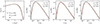 |
Fig. 1. Left panel: Unconditional first-crossing distribution for walks starting from S = 0, δ = 0. The histogram shows the results of random walks; the solid black and dashed orange curves show the ansatz (3) with q = 0.80 and q = 0.707, respectively; and the dotted grey curve shows the spherical collapse result. Other panels: Conditional first-crossing distribution at z > z0 for walks starting from S0 > 0 and δell(z0, S0) > 0 as indicated in the plot. The histogram again shows the results of random walks, the solid black curves show the ansatz (4), the dashed orange curves show the ansatz (3) with δsp(z)→δsp(z)−δsp(z0) and S → S − S0, and the dotted grey curve shows the spherical collapse result. |
For the conditional mass function, we studied random walks starting from S0 > 0 and δ0 = δell(S0, z0) > 0. The simplest ansatz for the first-crossing distribution pFC(S, z|S0, z0), as considered by Sheth & Tormen (2002), among others, is obtained by the shift δsp(z)→δsp(z)−δsp(z0) and S → S − S0 in (3). As seen in Fig. 1, comparing the orange dashed curves with the histograms, we find that this ansatz does not reproduce well the results of the random walks. A better estimate, shown by the solid black curves in Fig. 1, is given by
![Mathematical equation: $$ \begin{aligned} \begin{aligned}&p_{\rm FC}(S,z|S_0,z_0) = A^{\prime } \left[ 1 + \left(a \nu \right)^{-p}\right] \sqrt{\frac{\nu ^{\prime }}{2\pi }} \frac{e^{-\nu ^{\prime }/2} }{S-S_0} , \\&\nu = \frac{\delta _{\rm sp}(z)^2}{S} , \quad \nu ^{\prime } = \frac{(\delta _{\rm ell}(z,S_0)-\delta _{\rm ell}(z_0,S_0))^2}{S-S_0} , \end{aligned} \end{aligned} $$](/articles/aa/full_html/2025/10/aa55390-25/aa55390-25-eq5.gif) (4)
(4)
where, as in Eq. (2), a = 0.707 and the normalisation factor A′ in the limit z → z0 is
![Mathematical equation: $$ \begin{aligned} A^{\prime } = \left[1+\left(a \frac{\delta _{\rm sp}(z_0)^2}{S_0}\right)^{-p} \right]^{-1} . \end{aligned} $$](/articles/aa/full_html/2025/10/aa55390-25/aa55390-25-eq6.gif) (5)
(5)
In the limit z → z0, our formula (4) agrees well with the analytical estimate derived by Zhang et al. (2008). However, our expression also matches the numerical results for large redshift differences z − z0 ≫ 02.
From the first-crossing probabilities, we can construct the probability density that a halo whose mass at z′ is M′ ends up being a part of a halo of mass M > M′ at z < z′:
 (6)
(6)
This, in turn, directly gives the halo mass growth rate:
 (7)
(7)
Unlike the estimate derived by Correa et al. (2015), our estimate (7) accounts for the correction from ellipsoidal collapse. Moreover, our estimate is based on the expected increase in the halo mass, while the estimate of Correa et al. (2015) is based on finding the expected mass of the main progenitor. However, we find that these estimates agree within a factor of two across a broad range of halo masses and redshifts.
3. Dark matter models
3.1. Suppressed small-scale structures
We considered two DM models that predict suppression of small-scale structures: 1) FDM where the DM is provided by coherent waves of an ultra-light bosonic field with mass mFDM = 𝒪(10−20 eV) and 2) WDM where the DM is provided by semi-relativistic particles with masses mWDM = 𝒪(keV). The changes in the matter power spectrum in these cases can be described by transfer functions TJ(k)2, where J labels the model. The resulting matter power spectrum is given by
 (8)
(8)
where 𝒫CDM(k) denotes the CDM matter power spectrum that we compute with the transfer function from Eisenstein & Hu (1998).
In the case of FDM, the speed of sound is modified by quantum pressure, so that cs ∼ k/(4a2mFDM2). Consequently, the Jeans scale is non-zero (see e.g. Marsh (2016)),
![Mathematical equation: $$ \begin{aligned} k_{\rm J} = \frac{66.5\,\mathrm{Mpc}^{-1}}{(1+z_{\rm eq})^{1/4}} \left[\frac{\Omega _{\rm FDM}\,h^2}{0.12}\right]^{\frac{1}{4}}\left[\frac{m_{\rm FDM}}{10^{-22}\,\mathrm{eV}}\right]^{\frac{1}{2}}, \end{aligned} $$](/articles/aa/full_html/2025/10/aa55390-25/aa55390-25-eq10.gif) (9)
(9)
and perturbations at small scales k ≳ kJ are suppressed. This suppression can be estimated using an effective fluid approximation that is accurately matched to the solution of the Klein-Gordon equation (Hu et al. 2000; Passaglia & Hu 2022). We use the fitting formula provided by Passaglia & Hu (2022):
 (10)
(10)
where
 (11)
(11)
with m22 ≡ mFDM/10−22 eV.
In the case of WDM, a thermal production mechanism is typically assumed, and the particles are lighter than typical CDM particles and remain relativistic for a longer time. This implies that the free streaming length of WDM particles can be long, λfs ∼ (mWDM/keV)−4/3Mpc. In order to compute the resultant damping of the small-scale structures, it is necessary to track accurately the transition between relativistic and non-relativistic behaviour by solving the Boltzmann equations. This yields the fit (Bode et al. 2001; Hansen et al. 2002; Viel et al. 2005)
![Mathematical equation: $$ \begin{aligned} T_{\rm W} = \left[1+(\alpha k)^{2\mu }\right]^{-5/\mu } , \end{aligned} $$](/articles/aa/full_html/2025/10/aa55390-25/aa55390-25-eq13.gif) (12)
(12)
with μ = 1.12 and
![Mathematical equation: $$ \begin{aligned} \alpha = 0.049\left[\frac{m_{\rm WDM}}{\mathrm{keV}}\right]^{-1.11} \left[\frac{\Omega _{\rm DM}}{0.25}\right]^{0.11} \left[\frac{h}{0.7}\right]^{1.22} h^{-1} \mathrm{Mpc}. \end{aligned} $$](/articles/aa/full_html/2025/10/aa55390-25/aa55390-25-eq14.gif) (13)
(13)
3.2. Enhanced small-scale structures
For the enhancement of small-scale structures, we also considered two cases: 1) an axion DM model that includes axion mini-clusters and 2) a scenario where heavy primordial black holes (PBHs) constitute a fraction of the DM density. In both cases, we model the enhancement of the matter power spectrum as (Hütsi et al. 2023)
 (14)
(14)
This parametrisation includes one parameter, the scale kc above which the power spectrum is dominated by a white noise contribution. We performed the analysis in terms of kc, which is related to the parameters of the underlying DM models as discussed below.
In axion-like particle DM models, where the global U(1) symmetry is broken after cosmic inflation, significantly small-scale density fluctuations arise due to the Kibble mechanism. These lead to the formation of axion mini-clusters (Kolb & Tkachev 1993). This scenario results in a white noise contribution to the matter power spectrum (Fairbairn et al. 2018; Feix et al. 2019; Ellis et al. 2022). The resulting power spectrum can be approximated by Eq. (14) with
![Mathematical equation: $$ \begin{aligned} k_c \approx 3 h\, \mathrm{Mpc} ^{-1} \left[\frac{m_a}{10^{-18}\,\mathrm{eV} }\right]^{0.6} , \end{aligned} $$](/articles/aa/full_html/2025/10/aa55390-25/aa55390-25-eq16.gif) (15)
(15)
where ma denotes the axion-like particle mass. The white noise contribution is cut at scales that re-entered the horizon when the axion began oscillating:
 (16)
(16)
However, in the relevant part of the parameter space, the cut is far beyond the enhancement scale, kc ≪ kcut. We also note that the Jeans scale is larger than the cutoff scale, kJ > kcut.
In scenarios involving heavy PBHs there is a white noise contribution to the matter power spectrum (Inman & Ali-Haïmoud 2019; De Luca et al. 2020) with
![Mathematical equation: $$ \begin{aligned} k_c \approx 6 h \, \mathrm{Mpc} ^{-1} \left[\frac{f_{\rm PBH} m_{\rm PBH}}{10^4 M_\odot }\right]^{-0.4} , \end{aligned} $$](/articles/aa/full_html/2025/10/aa55390-25/aa55390-25-eq18.gif) (17)
(17)
where fPBH is the DM fraction in PBHs, mPBH is the PBH mass, and ρDM is the dark matter density. The cutoff is set by the average separation of PBHs (Hütsi et al. 2023):
![Mathematical equation: $$ \begin{aligned} \begin{aligned} k_{\rm cut}= 900 h \, \mathrm{Mpc} ^{-1} \left[f_{\rm PBH} \frac{10^4 M_\odot }{m_{\rm PBH}}\right]^{1/3} . \end{aligned} \end{aligned} $$](/articles/aa/full_html/2025/10/aa55390-25/aa55390-25-eq19.gif) (18)
(18)
Below this scale, one expects roughly one PBH per corresponding comoving volume, and the seed effect (Carr & Silk 1983, 2018; Cappelluti et al. 2022) becomes dominant. The condition kc < kcut is satisfied for fPBH > 10−4(mPBH/104 M⊙)−0.09.
3.3. Window function
In order to convert the matter power spectrum into the HMF, it is necessary to specify a window function to be used in conjunction with the excursion-set formalism. The window function is used to compute the variance of the matter perturbations,
 (19)
(19)
where the normalisation factor A is chosen to match the Planck measurement of σ8 = σ(R = 8/h Mpc) = 0.811 (Aghanim et al. 2020). We used a window function of the form (Leo et al. 2018; Verwohlt et al. 2024):
 (20)
(20)
where R is related to the mass of the overdensity by  . In the case of a suppressed matter power spectrum, the HMF scales as dn/dlnM ∝ Mc2/6 and the halo growth rate as dM/dz ∝ M1 − c2/6 at scales far below the suppression scale. For all models, we used c2 = 6 so that also for WDM and FDM models the growth rate increases with the halo mass, and fixed c1 = 0.43 so that the resulting variance in CDM closely matches that computed using the standard real space top hat window function, in agreement with simulation results. We find that this choice also reproduces well the simulation results in the FDM model (Schive et al. 2016), but it underestimates the halo mass where the HMF found in WDM simulations deviates from the CDM prediction (Lovell et al. 2014). On the other hand, the choice c1 = 1/3.3 suggested by Leo et al. (2018) reproduces the low-mass part, but it does not match the CDM prediction at high masses. To reproduce the simulation results in WDM and to match CDM predictions at masses much above the suppression scale, we used c1 = 0.43 in the window function and multiplied α in the WDM transfer function by 3.3c1 ≈ 1.4.
We show in the upper panel of Fig. 2 how the variance of the density perturbations in the models described above differs from that in the CDM model. For FDM and WDM, the variance asymptotes to a constant value at low masses. The break from the CDM-like behaviour at high masses is sharper for FDM than for WDM. This reflects the fact that the free streaming length does not make as abrupt a transition as the Jeans scale. For the case of enhanced perturbations, we see the opposite effect and the variance of the perturbation grows rapidly at low masses. In the lower panel of Fig. 2, we show the change in the DM halo growth rate for the different scenarios. In cases with suppressed small-scale structures, we find that the growth rate exceeds that of CDM, while the halos grow more slowly in the case with enhanced small-scale structures.
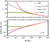 |
Fig. 2. Variance S = σ2 of matter perturbations (upper panel) and halo growth rate (lower panel) in the models considered in this work: CDM (dashed black line), FDM (green line), WDM (orange line), and an enhanced matter power spectrum (red line). |
The HMFs are shown in Fig. 3, where they are compared with the CDM predictions. For the case with suppressed small-scale structures, the HMF grows ∝M at low masses. This power-law behaviour does not significantly affect the fits to the UV luminosity observations discussed below. For the enhanced perturbations, we can see how the enhancement gets weaker at low z as the mini-clusters merge with heavier halos and their original imprint is diluted.
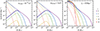 |
Fig. 3. HMF at various redshifts z in the FDM (left) and WDM (middle) models, and in models where white noise dominates the matter perturbations at k > kc (right). The dashed contours show the HMF in the CDM model for comparison. |
4. UV luminosity functions
After discussing the DM structures, which provide the potential wells that trap baryons, we now turn to the source of the UV light, namely the stars that populate galaxies. The stellar mass in a galaxy increases not only via mergers, but mainly via the formation of new stars from cold gas. At high z, the star formation rate (SFR) can be probed using the UV luminosity function, which quantifies the number density of galaxies as a function of their UV luminosity. The UV luminosity of a galaxy is directly proportional to the SFR because the sources that dominate this emission are massive 𝒪(10 M⊙) stars that are short-lived at cosmological scales, with τ ≲ 10 Myr3.
The observed UV luminosity function can be computed from the HMF as
 (21)
(21)
where dP(L|M)/dL denotes the distribution of luminosities emitted by galaxies in halos of mass M and dP(Lobs|L)/dLobs is the distribution of observed luminosities if the emitted luminosity is L. The latter is affected by gravitational lensing magnification (Takahashi et al. 2011) and dust attenuation (Wang & Heckman 1996):
 (22)
(22)
Here dP(B)/dB denotes the distribution of the dust attenuation B, and dP(μ)/dμ denotes the distribution of the lensing magnification μ.
4.1. Lensing magnification
The first correction to the observed luminosity that we consider is gravitational lensing. This correction is relevant for the bright end of the UV luminosity function, which receives contributions from magnified distant galaxies lensed by intervening structures. As shown by Takahashi et al. (2011), the magnification can be approximated as4
 (23)
(23)
where κ denotes the convergence given by the Laplacian of the lens potential. For multiple lenses, the convergence is obtained by summing the contributions from the different lenses j and subtracting the empty beam convergence κE,
 (24)
(24)
where Σj(rj) denotes the projected surface mass density of the jth lens, Dj the angular diameter distance of the lens, Ds the angular diameter distance of the source, and Dj, s the angular diameter distance between the lens and the source. The convergence of the jth lens depends on the mass of the lens Mj, the lens redshift zj, and the distance of the lens from the line of sight to the source rj, θj = {Mj, zj, rj}. As the mean convergence is ⟨κ⟩ = 0, the empty beam convergence can be written as κE = −⟨∑jκ(1)(θj)⟩.
We compute the distribution of μ by generating numerically the distribution of κ, converting it to dP(μ)/dμ using Eq. (23) and applying a 1/μ factor to transform the image-plane distribution into the source-plane distribution. We model the lenses by NFW halos whose spatial distribution follows a uniform distribution and use the halo mass-concentration/redshift relation derived by Ludlow et al. (2016). We account for the finite source sizes by averaging the surface density over a sphere of radius Rs that we obtained by projecting the source size to the lens plane. We fix the source size to 10 kpc (see in Takahashi et al. (2011), Ferrami & Wyithe (2023) how the result is affected by the source size). The distribution of lenses is given by
 (25)
(25)
To limit the number of lenses N, we impose an upper limit on the distance r of the halo from the line of sight, r < rmax(M, zl), so that κ(1) > κthr. We checked that our choice of κthr is sufficiently small that our results are insensitive to it. The distribution of contributions κ(1) is given by
 (26)
(26)
We compute the distribution of the convergence by picking random numbers from dP(1)(κ)/dκ to generate multiple realisations of ∑jκ(1)(θj) and shifting the resulting distribution by κE so that its mean is zero5.
The resulting distributions of lensing magnifications at different source redshifts are shown in Fig. 4. The distributions have a characteristic long tail towards high magnifications. This amplifies the high-luminosity (low-magnitude) tail of the UV luminosity functions, as seen in Fig. 5 by comparing the dashed and solid curves. We note that the lensing amplification is dominated by relatively heavy structures, M ≳ 1010 M⊙, and is not significantly affected by the changes in the small-scale structures that we consider in this work.
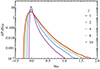 |
Fig. 4. Distributions of lensing magnifications at different source redshifts. |
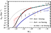 |
Fig. 5. UV luminosity function at z = 4 (black) and z = 17 (blue) with and without corrections due to lensing magnification and dust attenuation. The cyan and pink points show respectively the HST z = 4 data from Bouwens et al. (2021) and Harikane et al. (2022), and the brown and grey points the JWST z = 17 data from Pérez-González et al. (2025) and Castellano et al. (2025). |
4.2. Dust attenuation
Following the literature (see e.g. Trenti et al. (2015), Vogelsberger et al. (2020)), we neglect the variance in the dust attenuation B and approximate  . This gives
 (27)
(27)
where  .
.
The UV luminosity functions are commonly presented in terms of the absolute magnitude instead of the luminosity. The associated absolute magnitude MUV is defined by (Oke & Gunn 1983)
![Mathematical equation: $$ \begin{aligned} \log _{10}\left[\frac{L_{\rm UV}}{\mathrm{erg\,s^{-1}}}\right] = 0.4 \left(51.63-M_{\rm UV}\right), \end{aligned} $$](/articles/aa/full_html/2025/10/aa55390-25/aa55390-25-eq32.gif) (28)
(28)
where the normalisation is chosen to match the luminosity of the star Vega. Dust attenuation shifts the absolute magnitude by  , which we estimate as
![Mathematical equation: $$ \begin{aligned} A_{\rm UV} = \frac{1}{s} \ln \left[e^{s(C_0 + 0.2\ln 10 (C_1 \sigma _\beta )^2 + C_1 \bar{\beta }_{\rm UV})} + 1 \right], \end{aligned} $$](/articles/aa/full_html/2025/10/aa55390-25/aa55390-25-eq34.gif) (29)
(29)
with s = 3, C0 = 4.4, C1 = 2.0, σβ = 0.34, and
![Mathematical equation: $$ \begin{aligned} \bar{\beta }_{\rm UV} = -\exp \!\left[\frac{0.17(19.5+M_{\rm UV})}{1.54+0.075 z}\right] (1.54+0.075 z) . \end{aligned} $$](/articles/aa/full_html/2025/10/aa55390-25/aa55390-25-eq35.gif) (30)
(30)
The last is obtained by fitting the results shown in Table 3 of Bouwens et al. (2014), assuming that  scales exponentially with MUV. We note that, in Eq. (29), instead a piecewise function, we use a softplus function with sharpness parameter s = 3 chosen so that the resulting dust attenuation roughly matches that obtained by numerical sampling shown in Fig. 1 of Vogelsberger et al. (2020).
In terms of absolute magnitude, the UV luminosity function is given by
 (31)
(31)
where MUV = Mobs − AUV + 1.086lnμ. Comparing the short- and long-dashed curves in Fig. 5, we see that dust attenuation suppresses strongly the high-luminosity tail of the luminosity function at low redshifts, but at very high redshifts its effect is almost negligible. However, we note that the dust attenuation is calibrated to observations at z ≤ 8 (Bouwens et al. 2014) and we have simply extrapolated these results to z ≫ 8.
4.3. Star formation rate
We assume that the emitted UV magnitudes MUV in a given halo of mass M follow a Gaussian distribution:
![Mathematical equation: $$ \begin{aligned} \frac{\mathrm{d}P(M_{\rm UV}|M)}{\mathrm{d}M_{\rm UV}} = \frac{1}{\sqrt{2\pi } \sigma _{\rm UV}} \exp \left[ -\frac{(M_{\rm UV} - \bar{M}_{\rm UV})^2}{2\sigma _{\rm UV}^2} \right] . \end{aligned} $$](/articles/aa/full_html/2025/10/aa55390-25/aa55390-25-eq38.gif) (32)
(32)
The scatter in the MUV − M relation, σUV, is taken as a free parameter. The mean emitted UV luminosity,  , is directly proportional to the SFR:
 (33)
(33)
As mentioned in the Introduction, we assume that the SFR is proportional to the halo growth rate (Bian et al. 2013),  , where fB = ΩB/ΩM ≈ 0.16. We parametrise the proportionality coefficient f*(M), which models the feedback effects from SNe and AGNs, as a broken power law around M = Mc with an exponential suppression in halos with M < Mt < Mc,
 (34)
(34)
where α, β, ϵ > 0. A similar parametrisation is used in the GALLUMI code (Sabti et al. 2022a), for example. The difference is that in our parametrisation the maximum of f*(M) is at M = Mc for Mt ≪ Mc. We find that z-independent values of α, β, ϵ, and κUV give a good fit to the observations up to z ≈ 10, but that the data prefer higher luminosities at z ≳ 10.
To accommodate this enhancement in the luminosities of the early stars, we introduce a parametrisation in which the conversion factor κUV changes around z = zκ,
![Mathematical equation: $$ \begin{aligned} \kappa _{\rm UV} = \kappa _0 \left[\frac{1 + f_\kappa }{2} - \frac{1 - f_\kappa }{2} \tanh \left(\frac{z - z_\kappa }{\gamma }\right) \right] , \end{aligned} $$](/articles/aa/full_html/2025/10/aa55390-25/aa55390-25-eq43.gif) (35)
(35)
where κ0 = 1.15 × 10⁻²² M⊙ s erg−1 Myr−1, 0 < fκ ≤ 1, and γ > 0. The conversion factor depends on the initial stellar mass function and the value of κ0 corresponds to the Salpeter initial mass function (Madau & Dickinson 2014). We allow for a wide range of possibilities in the transition to Pop III stars: zκ determines the redshift at which the change of κUV starts, γ parametrises how sharp the transition is, and fκ is the fractional change in κ, such that at z ≫ zκ, κUV = fκκ0. We show κUV as a function of z for the best-fit values in the CDM model in the upper left panel of Fig. 6.
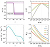 |
Fig. 6. Upper left: Best-fit UV conversion factor (35) as a function of redshift (thick purple curve) and the 68% range in fκ (purple band). Upper right: Best-fit SFR (34) as a function of halo mass at different redshifts. Lower left: SFR density with (solid) and without (dot-dashed) the suppression (36) of the feedback effects. Lower right: Best-fit mean UV magnitude as a function of the halo mass at different redshifts. |
In order to fit the highest-z UV data, we find that the feedback effects, which we parametrise with f*(M), need to be reduced. To allow for such a reduction, we parametrised the powers X = α, β so that they can approach zero linearly with z above some redshift zfb:
![Mathematical equation: $$ \begin{aligned} X_{z>z_{\rm fb}} = X \max \left[0, \frac{z_*-z}{z_*-z_{\rm fb}}\right] . \end{aligned} $$](/articles/aa/full_html/2025/10/aa55390-25/aa55390-25-eq44.gif) (36)
(36)
In this parametrisation, α and β become zero at z > z*, and f*(M) is mass independent at M ≫ Mt, as shown in the upper right panel of Fig. 6 for the best-fit values. This implies that in all halos with M ≫ Mt, the baryons that the halo accretes are converted into stars with efficiency ϵ.
In total, our parametrisation of the SFR, the UV conversion factor, and the distribution of the UV magnitudes includes 11 free parameters: {Mt, Mc, ϵ, α, β, γ, fκ, zκ, zfb, z*, σUV}.
5. Results
We considered UV luminosity function measurements derived from both HST observations (Bouwens et al. 2021; Harikane et al. 2022) and JWST observations (Donnan et al. 2024; Pérez-González et al. 2025; Castellano et al. 2025). The latter are based on high-z photometric measurements, most of which are not spectroscopically confirmed. This can lead to errors in the estimation of redshift. Most notably, a photometric measurement of CEERS-93316 indicated that this galaxy was at z ≈ 16 (Naidu et al. 2022a), but a later spectroscopic measurement revealed it to be at z ≈ 5 (Arrabal Haro et al. 2023). However, the redshifts of some of the high-z galaxies have been confirmed spectroscopically by Donnan et al. (2024).
We performed a Markov chain Monte Carlo (MCMC) analysis of the models. For each scan over the model parameters, we generated eight MCMC chains, each consisting of 12000 samples of which the first 2000 are discarded as burn-in. We used the Metropolis-Hastings sampler with Gaussian proposal distributions whose widths we chose so that the acceptance rate is around 10%. The model parameter priors are given in Table 1. We assumed that the data follow a split normal distribution 𝒩(μ, σ1, σ2), where μ denotes the mode and σ1, 2 the left- and right-hand side standard deviations. The likelihood is given by
 (37)
(37)
Parameter range and best-fit values.
where j represents the measurements and the function Φ(MUV, z) is the model prediction. The code used in the analysis is available at GitHub.
5.1. Cold dark matter
The full posteriors for our CDM fit parameters are shown in blue in Fig. 7 and the best-fit values are given in Table 1. We checked that the Gelman-Rubin statistic R (Gelman & Rubin 1992) is very close to 1 for each of the parameters. This indicates good convergence of the MCMC chains. The highest value, R ≈ 1.09, was obtained for log10(Mt/M⊙).
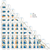 |
Fig. 7. Posteriors of SFR fits to the UV luminosity function observations in different models. The contours indicate the 68% and 95% credible regions. The marginalised 68% credible ranges and the 95% credible constraints are shown for CDM at the top of each column. |
Most of the parameters, in particular those parametrising the broken power-law shape of f*(M), are well constrained by the data, and the posteriors show only a mild negative correlation between α and β, and between α and Mc. The fits of α, β, and Mc are similar to those found by Harikane et al. (2022), but we find about a factor of two higher SFR. Compared to Sabti et al. (2022a), we fixed the cosmological parameters to the Planck CMB values, and we are able to constrain Mc and β better because the HST data we consider extend to higher luminosities.
From the posteriors of γ, fκ, and zκ, we see a clear (> 95%) preference for a relatively rapid change in κUV around zκ = 10 − 11 by factor of ∼3. The posterior of zfb shows that the preference for a high-z change in the powers α and β is less significant, < 95%. This is expected, since the change is driven by the measurements at z = 17 and z = 25 that have relatively large uncertainties and Φ = 0 is within the 95% range. Moreover, we see a correlation between fκ and zbf, indicating that the enhancement of the UV luminosity can be partly reduced by changing the powers α and β. The data prefer a narrow scatter in the UV magnitude, σUV < 0.15 at the 95% CL, and give an upper bound on the scale of the exponential SFR suppression, Mt < 109 M⊙, at the 95% CL. This implies that the explanation for the UV excess as a consequence of a large constant scatter in the (MUV, M) is disfavoured when compared to the Pop III star hypothesis6. This result should be treated with caution, however, since selection effects, which are not considered in the likelihood analysis, could modify the conclusion.
The evolution of κUV for the best fit is shown in the upper left panel of Fig. 6. The range shown in grey corresponds to estimates of the conversion factor for Pop III stars with top-heavy initial mass functions (Harikane et al. 2023). We see that the best fit prefers a sharp transition from Pop I and Pop II stars with standard Salpeter profiles up to z ∼ 10 to a top-heavy Pop III population at z > 10.8. The upper right panel of Fig. 6 illustrates how the feedback effects are suppressed for the best fit. This strongly enhances the SFR density,
 (38)
(38)
at high z, as shown in the lower left panel of Fig. 6. The lower right panel of Fig. 6 shows the relation between the mean UV magnitude and the halo mass at different redhifts.
In Fig. 8 we show the best-fit UV luminosity function in the CDM model (in black) compared with the HST and JWST observations at different redshifts. The change in the tail shape at MUV < −22 is primarily driven by the lensing magnification. The slight turn seen in the last panel at MUV > −18 is due to the exponential term in (34) that becomes relevant in the shown MUV range only at the highest z, as seen from the lower right panel of Fig. 6. The fit without the suppression of the feedback effects is shown by the dashed lines, and undershoots the measurements at z = 17 and 25. The dot-dashed curve shows the fit when the high-z enhancement in the luminosities is also removed. We see that this case undershoots the observed luminosity function at redshifts z > 10. Moreover, we see that our model does not provide a good fit of the brightest objects at z = 17. This may reflect a limitation of our parametrisation, but it is also possible that the luminosities of some of these objects are contaminated by AGNs (Castellano et al. 2025).
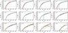 |
Fig. 8. UV luminosity function at different redshifts in the cold (black), fuzzy (green), and warm (orange) DM models and in the model with enhanced matter power (red). The best fit is shown for CDM and WDM cases, while for FDM the mass corresponds to the 95% lower bound. The dashed and dot-dashed curves show the CDM UV luminosity function without the suppression of the feedback effects and without the change in the UV conversion factor κUV. The points with errorbars show the HST measurements from Bouwens et al. (2021) (cyan) and Harikane et al. (2022) (pink) and the JWST measurements from Donnan et al. (2024) (blue), Pérez-González et al. (2025) (brown), and Castellano et al. (2025) (grey). |
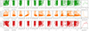 |
Fig. 9. Posteriors of SFR fits to the UV luminosity function observations as a function of FDM mass (top panels), WDM mass (middle panels), and the enhancement scale (bottom panels). The contours indicate the 68% and 95% credible regions. |
5.2. Suppressed small-scale perturbations
We also see in Fig. 8 the comparison between the UV data and the predictions with suppressed small-scale structures in the FDM (green) and WDM (orange) models. For FDM we show the case where the model parameters correspond to the CDM best fit and the FDM mass is at the 95% CL lower limit, while for WDM we show the best fit case, which is slightly better than in the CDM model. We see that the predictions are indistinguishable for z ≲ 10, and up to z ∼ 15 the suppression is at lighter halos (bigger MUV) than the observations can probe. At the highest redshifts, z > 15, we see that the model predictions undershoot the observations. However, since the uncertainties in the data are large, the observations at high z are compatible with a strongly suppressed UV luminosity function.
For the FDM model, the parameters for the star formation rate, the enhancement of the UV luminosity and the suppression of the feedback effects remain the same as in the CDM model, as seen in the posterior plots in Fig. 7. This reflects the fact that the FDM prediction deviates sharply from the CDM prediction at the suppression scale. The main difference between FDM and CDM models is seen in z*, which determines when the feedback effects are fully removed. For low FDM masses the feedback effects can be fully removed at lower z because the luminosity function is suppressed by the FDM quantum pressure, which causes the peak in the posterior of the FDM mass shown in the top panels of Fig. 9. The posterior also shows a lower bound on the FDM mass, mFDM > 5.6 × 10⁻²² eV at 95% CL. The UV luminosity function has been previously studied in the FDM model (Bozek et al. 2015; Schive et al. 2016; Corasaniti et al. 2017; Winch et al. 2024). Our constraint on the FDM mass is somewhat stronger than that obtained by Winch et al. (2024) using the HST data and JWST data from Harikane et al. (2024).
The deviation from the CDM prediction is smoother in the WDM case, and starts far above the half-mode mass. Consequently, the WDM fit at small mWDM moves to smaller values of α and larger values of β than in the CDM model, as seen in the posterior plots in Figs. 7 and 9. Due to the degeneracy between α and mWDM, in particular, the WDM model favours a narrow mass range around 2 keV. The maximum likelihood in the WDM model is slightly higher than in CDM, Δlnℒ ≈ 2.7, and the Bayesian information criterion (BIC), which accounts for the increase in the number of parameters, indicates a mild (insignificant) preference for WDM over CDM with ΔBIC ≈ −0.4. As seen from Fig. 8, the fit improves in particular at z = 17.
The posteriors of the WDM mass shown in the middle panels of Fig. 9 show a lower bound mWDM > 1.5 keV at 95% CL. Several previous works have derived constraints on WDM from UV luminosity function observations (Menci et al. 2016; Corasaniti et al. 2017; Rudakovskyi et al. 2021; Hibbard et al. 2022; Maio & Viel 2023; Liu et al. 2024). Although we used a larger set of JWST data, the bound on the WDM mass is weaker than that found by Liu et al. (2024). This difference arises because Liu et al. (2024) uses a low-z fit of the HMF to numerical simulations derived in Stücker et al. (2021), while we estimate the WDM HMF using the transfer function and the smooth-k window function.
5.3. Enhanced small-scale perturbations
Enhancing the small-scale structure has the opposite effect to WDM or FDM, but the conclusions are very similar. We see in Fig. 8 that for z ≲ 10 the predictions resemble those of CDM, and only at the highest redshifts do we see a small enhancement of the UV luminosity function that grows at lower scales, MUV ≲ −20. This reflects the fact that the higher the redshift, the more deviations from CDM one can expect to see, especially for low-mass halos. When fitting the star formation parameters, the results are independent of the enhancement of the scales and very similar to CDM, as seen in Fig. 7. We conclude that enhancing the matter power spectrum does not help to explain the excess in the UV radiation at high z when other possibilities (e.g. Pop III stars) are taken into account. The fit favours a sharp transition to Pop III stars and such a feature cannot be reproduced by enhancing the matter power spectrum. The fit gives a lower bound of kc > 25 Mpc−1 at 95% CL, as seen in the bottom panels of Fig. 9. The excluded region corresponds to axion mini-clusters produced with ma < 6.6 × 10⁻¹⁷ eV or PBHs that obey fPBH > max[105 M⊙/mPBH, 10−4(mPBH/104 M⊙)−0.09], where the second bound comes from the requirement that kc < kcut. Our constraint on kc is significantly stronger than that implied by the measurements of the matter power spectrum at scales 0.5 < k/Mpc−1 < 10 derived by Sabti et al. (2022b) and that implied by the analysis of Iršič et al. (2020), both using the HST data alone. For PBHs, our constraint is stronger than that derived by Murgia et al. (2019), which considered the limit on an enhanced small-scale power spectrum imposed by the Lyman-α forest observations. In Fig. 10, we show a compilation of previous PBH constraints together with our new constraint in red.
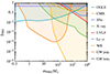 |
Fig. 10. Constraints on the fraction of the DM density provided by PBHs from the OGLE microlensing survey (Mróz et al. 2024), accretion limits from CMB observations (Serpico et al. 2020), SNe lensing (Zumalacarregui & Seljak 2018), the population of X-ray sources (Inoue & Kusenko 2017), Lyman-α data (Murgia et al. 2019), survival of wide binaries (Monroy-Rodríguez & Allen 2014), the population of gravitational wave (GW) sources (Andrés-Carcasona et al. 2024), and GW lensing (Urrutia et al. 2023). The red line shows the upper limit derived in this work from measurements of the UV luminosity function. |
6. Conclusions
We have investigated in this work the implications of the high-z UV luminosity function observations with HST and JWST for star formation and different DM models. We have revisited the excursion-set formalism to compute the unconditional and conditional halo mass functions and derived a new estimate of the halo growth rate. We have also proposed a new window function, inspired by the smooth-k Leo et al. (2018) window function, which reproduces well the numerical results and matches better the CDM predictions at high masses.
We have found that, assuming that the SFR is proportional to the halo growth rate, the observations of the UV luminosity function indicate two interesting effects that change the luminosity function at high z. First, we find evidence at more than 95% CL for a sharp enhancement in the luminosity function around z ≃ 10. This can be explained by a transition from a Salpeter mass function to a top-heavy Pop III mass function. Beyond z = 10 − 15 the luminosity function needs to be further enhanced, in particular to match the JWST observations at z = 17 and 25. This enhancement can be achieved by reducing the feedback from SNe and AGNs. The evidence for this second effect is, however, less than 95% CL. We have also considered the effect of dust attenuation and lensing, and shown that they are relevant for the bright end of the luminosity function at z < 10, but do not play a significant role in fitting the higher-redshift data.
We have considered departures from CDM in two directions, suppressing the small-scale structures via either warm or fuzzy DM and enhancing the matter power spectrum with white noise, which could happen in scenarios that include axion mini-clusters or PBHs. When marginalising over the SFR parametrisation, we find a lower bound of 5.6 × 10⁻²²eV for the FDM mass and 1.5 keV for the WDM mass, at 95% CL. Because the new JWST data at high z still have significant uncertainties, we find that the DM bounds are not much stronger than those obtained using the HST data alone. Another important conclusion is that enhanced matter perturbations are not preferred over changes in the star formation rate due to the presence of Pop III stars and changes in the feedback in the pre-reionisation era. We have found that the data constrain the scale of the enhancement to kc > 25 Mpc−1 at 95% CL, excluding, for example, the possibility of axion mini-clusters produced for ma < 6.6 × 10⁻¹⁷ eV or heavy PBHs that constitute a fraction fPBH > max[105 M⊙/mPBH, 10−4(mPBH/104 M⊙)−0.09] of DM. As JWST gathers more data and the uncertainties are reduced, the bounds on DM will become significantly stronger and our knowledge of star formation at high z will improve. In a forthcoming paper we will leverage our findings to compute the growth of SMBHs in non-CDM scenarios and obtain more competitive bounds on deviations from CDM using the measurements of high-z SMBHs by JWST.
The spherical collapse model corresponds to p = 0, q = 1, and A = 1/2.
The ellipsoidal collapse thresholds at different redshifts can intersect; however, this occurs only at very small halo masses, M < 104 M⊙, which are not relevant for our study.
The timescale is further reduced if the Pop III mass function is more top-heavy.
This approximation underestimates the high-μ tail of the distribution. However, this tail is damped by the finite sizes of the lenses.
A similar approach of finding the distribution of a sum of random variables was introduced by Ellis et al. (2024) for the computation of the gravitational wave background from a population of supermassive black hole binaries.
However, a mass-dependent scatter that increases at small halo masses could enhance the UV luminosities at high z (Gelli et al. 2024).
Acknowledgments
This work was supported by the Estonian Research Council grants PRG803, PSG869, RVTT3 and RVTT7 and the Center of Excellence program TK202. The work of J.E. and M.F. was supported by the United Kingdom STFC Grants ST/T000759/1 and ST/X000753/1. The work of V.V. was partially supported by the European Union’s Horizon Europe research and innovation program under the Marie Skłodowska-Curie grant agreement No. 101065736.
References
- Aghanim, N., Akrami, Y., Ashdown, M., et al. 2020, A&A, 641, A6 [Erratum: Astron. Astrophys. 652, C4 (2021)] [NASA ADS] [CrossRef] [EDP Sciences] [Google Scholar]
- Andrés-Carcasona, M., Iovino, A. J., Vaskonen, V., et al. 2024, Phys. Rev. D, 110, 023040 [Google Scholar]
- Arrabal Haro, P., Dickinson, M., Finkelstein, S. L., et al. 2023, Nature, 622, 707 [NASA ADS] [CrossRef] [Google Scholar]
- Bagley, M. B., Finkelstein, S. L., Rojas-Ruiz, S., et al. 2024, ApJ, 961, 209 [NASA ADS] [CrossRef] [Google Scholar]
- Bian, F., Fan, X., Jiang, L., et al. 2013, ApJ, 774, 28 [Google Scholar]
- Bode, P., Ostriker, J. P., & Turok, N. 2001, ApJ, 556, 93 [Google Scholar]
- Bond, J. R., Cole, S., Efstathiou, G., & Kaiser, N. 1991, ApJ, 379, 440 [NASA ADS] [CrossRef] [Google Scholar]
- Bouwens, R. J., Illingworth, G. D., Oesch, P. A., et al. 2014, ApJ, 793, 115 [Google Scholar]
- Bouwens, R. J., Oesch, P. A., Stefanon, M., et al. 2021, AJ, 162, 47 [NASA ADS] [CrossRef] [Google Scholar]
- Bouwens, R. J., Stefanon, M., Brammer, G., et al. 2023, MNRAS, 523, 1036 [NASA ADS] [CrossRef] [Google Scholar]
- Bozek, B., Marsh, D. J. E., Silk, J., & Wyse, R. F. G. 2015, MNRAS, 450, 209 [NASA ADS] [CrossRef] [Google Scholar]
- Cappelluti, N., Hasinger, G., & Natarajan, P. 2022, ApJ, 926, 205 [NASA ADS] [CrossRef] [Google Scholar]
- Carr, B. J., & Silk, J. 1983, ApJ, 268, 1 [Google Scholar]
- Carr, B., & Silk, J. 2018, MNRAS, 478, 3756 [NASA ADS] [CrossRef] [Google Scholar]
- Castellano, M., Fontana, A., Treu, T., et al. 2023, ApJ, 948, L14 [NASA ADS] [CrossRef] [Google Scholar]
- Castellano, M., Fontana, A., Merlin, E., et al. 2025, A&A, submitted [arXiv:2504.05893] [Google Scholar]
- Chakraborty, A., & Choudhury, T. R. 2024, JCAP, 07, 078 [Google Scholar]
- Corasaniti, P. S., Agarwal, S., Marsh, D. J. E., & Das, S. 2017, Phys. Rev. D, 95, 083512 [NASA ADS] [CrossRef] [Google Scholar]
- Correa, C. A., Wyithe, J. S. B., Schaye, J., & Duffy, A. R. 2015, MNRAS, 450, 1514 [NASA ADS] [CrossRef] [Google Scholar]
- De Luca, V., Desjacques, V., Franciolini, G., & Riotto, A. 2020, JCAP, 11, 028 [Google Scholar]
- Dekel, A., Sarkar, K. C., Birnboim, Y., Mandelker, N., & Li, Z. 2023, MNRAS, 523, 3201 [NASA ADS] [CrossRef] [Google Scholar]
- Dodelson, S. 2003, Modern Cosmology (Amsterdam: Academic Press) [Google Scholar]
- Donnan, C. T., McLeod, D. J., Dunlop, J. S., et al. 2023, MNRAS, 518, 6011 [Google Scholar]
- Donnan, C. T., McLure, R. J., Dunlop, J. S., et al. 2024, MNRAS, 533, 3222 [NASA ADS] [CrossRef] [Google Scholar]
- Eisenstein, D. J., & Hu, W. 1998, ApJ, 496, 605 [Google Scholar]
- Ellis, D., Marsh, D. J. E., Eggemeier, B., et al. 2022, Phys. Rev. D, 106, 103514 [Google Scholar]
- Ellis, J., Fairbairn, M., Hütsi, G., et al. 2024, Phys. Rev. D, 109, L021302 [NASA ADS] [CrossRef] [Google Scholar]
- Fairbairn, M., Marsh, D. J. E., Quevillon, J., & Rozier, S. 2018, Phys. Rev. D, 97, 083502 [Google Scholar]
- Feix, M., Frank, J., Pargner, A., et al. 2019, JCAP, 05, 021 [Google Scholar]
- Ferrami, G., & Wyithe, J. S. B. 2023, MNRAS, 523, L21 [Google Scholar]
- Finkelstein, S. L., Bagley, M., Song, M., et al. 2022, ApJ, 928, 52 [CrossRef] [Google Scholar]
- Fujimoto, S., Naidu, R. P., Chisholm, J., et al. 2025, ApJ, 989, 46 [Google Scholar]
- Fukushima, H., & Yajima, H. 2021, MNRAS, 506, 5512 [NASA ADS] [CrossRef] [Google Scholar]
- Gelli, V., Mason, C., & Hayward, C. C. 2024, ApJ, 975, 192 [NASA ADS] [CrossRef] [Google Scholar]
- Gelman, A., & Rubin, D. B. 1992, Statist. Sci., 7, 457 [NASA ADS] [Google Scholar]
- Hansen, S. H., Lesgourgues, J., Pastor, S., & Silk, J. 2002, MNRAS, 333, 544 [Google Scholar]
- Harikane, Y., Ono, Y., Ouchi, M., et al. 2022, ApJS, 259, 20 [NASA ADS] [CrossRef] [Google Scholar]
- Harikane, Y., Ouchi, M., Oguri, M., et al. 2023, ApJS, 265, 5 [NASA ADS] [CrossRef] [Google Scholar]
- Harikane, Y., Nakajima, K., Ouchi, M., et al. 2024, ApJ, 960, 56 [NASA ADS] [CrossRef] [Google Scholar]
- Hibbard, J. J., Mirocha, J., Rapetti, D., et al. 2022, ApJ, 929, 151 [NASA ADS] [CrossRef] [Google Scholar]
- Hirano, S., Hosokawa, T., Yoshida, N., et al. 2014, ApJ, 781, 60 [NASA ADS] [CrossRef] [Google Scholar]
- Hirano, S., Hosokawa, T., Yoshida, N., Omukai, K., & Yorke, H. W. 2015, MNRAS, 448, 568 [NASA ADS] [CrossRef] [Google Scholar]
- Hu, W., Barkana, R., & Gruzinov, A. 2000, Phys. Rev. Lett., 85, 1158 [NASA ADS] [CrossRef] [Google Scholar]
- Hütsi, G., Raidal, M., Urrutia, J., Vaskonen, V., & Veermäe, H. 2023, Phys. Rev. D, 107, 043502 [CrossRef] [Google Scholar]
- Inman, D., & Ali-Haïmoud, Y. 2019, Phys. Rev. D, 100, 083528 [NASA ADS] [CrossRef] [Google Scholar]
- Inoue, Y., & Kusenko, A. 2017, JCAP, 10, 034 [Google Scholar]
- Iršič, V., Xiao, H., & McQuinn, M. 2020, Phys. Rev. D, 101, 123518 [Google Scholar]
- Jiang, F., & van den Bosch, F. C. 2014, MNRAS, 440, 193 [CrossRef] [Google Scholar]
- Klessen, R. S., & Glover, S. C. O. 2023, ARA&A, 61, 65 [NASA ADS] [CrossRef] [Google Scholar]
- Kolb, E. W., & Tkachev, I. I. 1993, Phys. Rev. Lett., 71, 3051 [NASA ADS] [CrossRef] [Google Scholar]
- Leethochawalit, N., Roberts-Borsani, G., Morishita, T., Trenti, M., & Treu, T. 2023, MNRAS, 524, 5454 [NASA ADS] [CrossRef] [Google Scholar]
- Leo, M., Baugh, C. M., Li, B., & Pascoli, S. 2018, JCAP, 04, 010 [Google Scholar]
- Liu, B., Shan, H., & Zhang, J. 2024, ApJ, 968, 79 [Google Scholar]
- Lovell, M. R., Frenk, C. S., Eke, V. R., et al. 2014, MNRAS, 439, 300 [Google Scholar]
- Ludlow, A. D., Bose, S., Angulo, R. E., et al. 2016, MNRAS, 460, 1214 [Google Scholar]
- Madau, P., & Dickinson, M. 2014, ARA&A, 52, 415 [Google Scholar]
- Maio, U., & Viel, M. 2023, A&A, 672, A71 [NASA ADS] [CrossRef] [EDP Sciences] [Google Scholar]
- Maiolino, R., Úbler, H., Perna, M., et al. 2024, A&A, 687, A67 [NASA ADS] [CrossRef] [EDP Sciences] [Google Scholar]
- Marsh, D. J. E. 2016, Phys. Rept., 643, 1 [NASA ADS] [CrossRef] [Google Scholar]
- McLeod, D. J., McLure, R. J., & Dunlop, J. S. 2016, MNRAS, 459, 3812 [NASA ADS] [CrossRef] [Google Scholar]
- Menci, N., Grazian, A., Castellano, M., & Sanchez, N. G. 2016, ApJ, 825, L1 [Google Scholar]
- Monroy-Rodríguez, M. A., & Allen, C. 2014, ApJ, 790, 159 [CrossRef] [Google Scholar]
- Morishita, T., & Stiavelli, M. 2023, ApJ, 946, L35 [NASA ADS] [CrossRef] [Google Scholar]
- Mróz, P., Udalski, A., Szymanski, M. K., et al. 2024, Nature, 632, 749 [CrossRef] [Google Scholar]
- Murgia, R., Scelfo, G., Viel, M., & Raccanelli, A. 2019, Phys. Rev. Lett., 123, 071102 [Google Scholar]
- Naidu, R. P., Oesch, P. A., Setton, D. J., et al. 2022a, arXiv e-prints [arXiv:2208.02794] [Google Scholar]
- Naidu, R. P., Oesch, P. A., van Dokkum, P., et al. 2022b, ApJ, 940, L14 [NASA ADS] [CrossRef] [Google Scholar]
- Oesch, P. A., Bouwens, R. J., Illingworth, G. D., Labbé, I., & Stefanon, M. 2018, ApJ, 855, 105 [Google Scholar]
- Oke, J. B., & Gunn, J. E. 1983, ApJ, 266, 713 [NASA ADS] [CrossRef] [Google Scholar]
- Parashari, P., & Laha, R. 2023, MNRAS, 526, L63 [NASA ADS] [CrossRef] [Google Scholar]
- Passaglia, S., & Hu, W. 2022, Phys. Rev. D, 105, 123529 [Google Scholar]
- Pérez-González, P. G., et al. 2025, arXiv e-prints [arXiv:2503.15594] [Google Scholar]
- Pérez-González, P. G., Costantin, L., Langeroodi, D., et al. 2023, ApJ, 951, L1 [CrossRef] [Google Scholar]
- Reed, D., Gardner, J., Quinn, T., et al. 2003, MNRAS, 346, 565 [NASA ADS] [CrossRef] [Google Scholar]
- Rudakovskyi, A., Mesinger, A., Savchenko, D., & Gillet, N. 2021, MNRAS, 507, 3046 [NASA ADS] [CrossRef] [Google Scholar]
- Sabti, N., Muñoz, J. B., & Blas, D. 2022a, Phys. Rev. D, 105, 043518 [Google Scholar]
- Sabti, N., Muñoz, J. B., & Blas, D. 2022b, ApJ, 928, L20 [Google Scholar]
- Schive, H.-Y., Chiueh, T., Broadhurst, T., & Huang, K.-W. 2016, ApJ, 818, 89 [NASA ADS] [CrossRef] [Google Scholar]
- Serpico, P. D., Poulin, V., Inman, D., & Kohri, K. 2020, Phys. Rev. Res., 2, 023204 [NASA ADS] [CrossRef] [Google Scholar]
- Sheth, R. K., & Tormen, G. 1999, MNRAS, 308, 119 [Google Scholar]
- Sheth, R. K., & Tormen, G. 2002, MNRAS, 329, 61 [Google Scholar]
- Sheth, R. K., Mo, H. J., & Tormen, G. 2001, MNRAS, 323, 1 [NASA ADS] [CrossRef] [Google Scholar]
- Sipple, J., Lidz, A., Grin, D., & Sun, G. 2025, MNRAS, 538, 1830 [Google Scholar]
- Steinhardt, C. L., Kokorev, V., Rusakov, V., Garcia, E., & Sneppen, A. 2023, ApJ, 951, L40 [NASA ADS] [CrossRef] [Google Scholar]
- Stücker, J., Angulo, R. E., Hahn, O., & White, S. D. M. 2021, MNRAS, 509, 1703 [Google Scholar]
- Susa, H., & Umemura, M. 2004, ApJ, 600, 1 [Google Scholar]
- Takahashi, R., Oguri, M., Sato, M., & Hamana, T. 2011, ApJ, 742, 15 [NASA ADS] [CrossRef] [Google Scholar]
- Trenti, M., Perna, R., & Jimenez, R. 2015, ApJ, 802, 103 [Google Scholar]
- Urrutia, J., Vaskonen, V., & Veermäe, H. 2023, Phys. Rev. D, 108, 023507 [Google Scholar]
- Vanzella, E., Loiacono, F., Bergamini, P., et al. 2023, A&A, 678, A173 [NASA ADS] [CrossRef] [EDP Sciences] [Google Scholar]
- Ventura, E. M., Qin, Y., Balu, S., & Wyithe, J. S. B. 2024, MNRAS, 529, 628 [Google Scholar]
- Verwohlt, J., Mason, C. A., Muñoz, J. B., et al. 2024, Phys. Rev. D, 110, 103533 [Google Scholar]
- Viel, M., Lesgourgues, J., Haehnelt, M. G., Matarrese, S., & Riotto, A. 2005, Phys. Rev. D, 71, 063534 [NASA ADS] [CrossRef] [Google Scholar]
- Vogelsberger, M., Nelson, D., Pillepich, A., et al. 2020, MNRAS, 492, 5167 [NASA ADS] [CrossRef] [Google Scholar]
- Wang, B., & Heckman, T. M. 1996, ApJ, 457, 645 [Google Scholar]
- Winch, H., Rogers, K. K., Hložek, R., & Marsh, D. J. E. 2024, ApJ, 976, 40 [NASA ADS] [CrossRef] [Google Scholar]
- Yung, L. Y. A., Somerville, R. S., & Iyer, K. G. 2025, arXiv e-prints [arXiv:2504.18618] [Google Scholar]
- Zhang, J., Ma, C.-P., & Fakhouri, O. 2008, MNRAS, 387, L13 [CrossRef] [Google Scholar]
- Zheng, H., Bose, S., Frenk, C. S., et al. 2024, MNRAS, 528, 7300 [Google Scholar]
- Zumalacarregui, M., & Seljak, U. 2018, Phys. Rev. Lett., 121, 141101 [Google Scholar]
All Tables
All Figures
|
Fig. 1. Left panel: Unconditional first-crossing distribution for walks starting from S = 0, δ = 0. The histogram shows the results of random walks; the solid black and dashed orange curves show the ansatz (3) with q = 0.80 and q = 0.707, respectively; and the dotted grey curve shows the spherical collapse result. Other panels: Conditional first-crossing distribution at z > z0 for walks starting from S0 > 0 and δell(z0, S0) > 0 as indicated in the plot. The histogram again shows the results of random walks, the solid black curves show the ansatz (4), the dashed orange curves show the ansatz (3) with δsp(z)→δsp(z)−δsp(z0) and S → S − S0, and the dotted grey curve shows the spherical collapse result. |
| In the text | |
|
Fig. 2. Variance S = σ2 of matter perturbations (upper panel) and halo growth rate (lower panel) in the models considered in this work: CDM (dashed black line), FDM (green line), WDM (orange line), and an enhanced matter power spectrum (red line). |
| In the text | |
|
Fig. 3. HMF at various redshifts z in the FDM (left) and WDM (middle) models, and in models where white noise dominates the matter perturbations at k > kc (right). The dashed contours show the HMF in the CDM model for comparison. |
| In the text | |
|
Fig. 4. Distributions of lensing magnifications at different source redshifts. |
| In the text | |
|
Fig. 5. UV luminosity function at z = 4 (black) and z = 17 (blue) with and without corrections due to lensing magnification and dust attenuation. The cyan and pink points show respectively the HST z = 4 data from Bouwens et al. (2021) and Harikane et al. (2022), and the brown and grey points the JWST z = 17 data from Pérez-González et al. (2025) and Castellano et al. (2025). |
| In the text | |
|
Fig. 6. Upper left: Best-fit UV conversion factor (35) as a function of redshift (thick purple curve) and the 68% range in fκ (purple band). Upper right: Best-fit SFR (34) as a function of halo mass at different redshifts. Lower left: SFR density with (solid) and without (dot-dashed) the suppression (36) of the feedback effects. Lower right: Best-fit mean UV magnitude as a function of the halo mass at different redshifts. |
| In the text | |
|
Fig. 7. Posteriors of SFR fits to the UV luminosity function observations in different models. The contours indicate the 68% and 95% credible regions. The marginalised 68% credible ranges and the 95% credible constraints are shown for CDM at the top of each column. |
| In the text | |
|
Fig. 8. UV luminosity function at different redshifts in the cold (black), fuzzy (green), and warm (orange) DM models and in the model with enhanced matter power (red). The best fit is shown for CDM and WDM cases, while for FDM the mass corresponds to the 95% lower bound. The dashed and dot-dashed curves show the CDM UV luminosity function without the suppression of the feedback effects and without the change in the UV conversion factor κUV. The points with errorbars show the HST measurements from Bouwens et al. (2021) (cyan) and Harikane et al. (2022) (pink) and the JWST measurements from Donnan et al. (2024) (blue), Pérez-González et al. (2025) (brown), and Castellano et al. (2025) (grey). |
| In the text | |
|
Fig. 9. Posteriors of SFR fits to the UV luminosity function observations as a function of FDM mass (top panels), WDM mass (middle panels), and the enhancement scale (bottom panels). The contours indicate the 68% and 95% credible regions. |
| In the text | |
|
Fig. 10. Constraints on the fraction of the DM density provided by PBHs from the OGLE microlensing survey (Mróz et al. 2024), accretion limits from CMB observations (Serpico et al. 2020), SNe lensing (Zumalacarregui & Seljak 2018), the population of X-ray sources (Inoue & Kusenko 2017), Lyman-α data (Murgia et al. 2019), survival of wide binaries (Monroy-Rodríguez & Allen 2014), the population of gravitational wave (GW) sources (Andrés-Carcasona et al. 2024), and GW lensing (Urrutia et al. 2023). The red line shows the upper limit derived in this work from measurements of the UV luminosity function. |
| In the text | |
Current usage metrics show cumulative count of Article Views (full-text article views including HTML views, PDF and ePub downloads, according to the available data) and Abstracts Views on Vision4Press platform.
Data correspond to usage on the plateform after 2015. The current usage metrics is available 48-96 hours after online publication and is updated daily on week days.
Initial download of the metrics may take a while.