| Issue |
A&A
Volume 702, October 2025
|
|
|---|---|---|
| Article Number | A105 | |
| Number of page(s) | 13 | |
| Section | Cosmology (including clusters of galaxies) | |
| DOI | https://doi.org/10.1051/0004-6361/202555522 | |
| Published online | 10 October 2025 | |
Estimating the heterogeneity of pressure profiles within a complete sample of 55 galaxy clusters: A Bayesian hierarchical model
1
INAF-Osservatorio Astronomico di Brera, via Brera 28, 20121 Milano, Italy
2
Insubria University, Department of Pure and Applied Sciences, Computer Science Division, via Ottorino Rossi, 21100 Varese, Italy
3
INAF-Osservatorio Astronomico di Brera, via Emilio Bianchi 46, 23807 Merate, Italy
⋆ Corresponding author: This email address is being protected from spambots. You need JavaScript enabled to view it.
Received:
15
May 2025
Accepted:
7
August 2025
Abstract
Galaxy clusters exhibit heterogeneity in their pressure profiles, even after rescaling, highlighting the need for adequately sized samples to accurately capture variations across the cluster population. We present a Bayesian hierarchical model that simultaneously fits individual cluster parameters and the underlying population distribution, providing estimates of the population-averaged pressure profile and the intrinsic scatter, as well as accurate pressure estimates for individual objects. We introduce a highly flexible, low-covariance, and interpretable parametrization of the pressure profile based on restricted cubic splines. We model the scatter properly accounting for outliers, and we incorporate corrections for beam and transfer function, as is required for Sunyaev-Zel’dovich (SZ) data. Our model is applied to the largest non-stacked sample of individual cluster radial profiles, extracted from SPT+Planck Compton-y maps. This is a complete sample of 55 clusters, with 0.05 < z < 0.30 and M500 > 4 × 10¹⁴ M⊙, enabling subdivision into sizable morphological classes based on eROSITA data. Fitting is computationally feasible within a few days on a modern (2024) personal computer. The shape of the population-averaged pressure profile, at our 250 kpc full width at half maximum resolution, closely resembles the universal pressure profile, despite the flexibility of our model for accommodating alternative shapes, with a ∼12% lower normalization, similar to what is needed to alleviate the tension between cosmological parameters derived from the cosmic microwave background and Planck SZ cluster counts. Beyond r500, our pressure profile is steeper than previous determinations. The intrinsic scatter is consistent with or lower than previous estimates, despite the broader diversity expected from our SZ selection. Our flexible pressure modelization identifies a few clusters with nonstandard concavity in their radial profiles but no outliers in amplitude. When dividing the sample by morphology, we find remarkably similar pressure profiles across classes, though regular clusters show evidence of lower scatter and a more centrally peaked profile compared to disturbed ones.
Key words: methods: statistical / galaxies: clusters: general / galaxies: clusters: intracluster medium
© The Authors 2025
 Open Access article, published by EDP Sciences, under the terms of the Creative Commons Attribution License (https://creativecommons.org/licenses/by/4.0), which permits unrestricted use, distribution, and reproduction in any medium, provided the original work is properly cited.
This article is published in open access under the Subscribe to Open model. This email address is being protected from spambots. You need JavaScript enabled to view it. to support open access publication.
1. Introduction
Galaxy clusters are the largest gravitationally bound objects in the Universe and, as such, play a crucial role in the study of cosmic evolution on the largest scales (Kravtsov & Borgani 2012). The Sunyaev-Zeldovich effect (SZ, Sunyaev & Zeldovich 1970, 1972) in the cosmic microwave background (CMB) is an ideal direct tracer of the gas pressure in the intra-cluster medium (ICM) of galaxy clusters. The hot gas trapped within the cluster’s gravitational potential leaves an imprint on the microwave sky as its Compton free electrons scatter the photons of the CMB radiation. The SZ effect depends directly on the integrated pressure along the line of sight, making it an ideal probe of the distribution of pressure across the ICM of galaxy clusters. This helps constrain models of structure formation for different cosmological scenarios (Pratt et al. 2019; Bocquet et al. 2024).
Estimating the average pressure profile of a galaxy cluster population, along with its dispersion, provides valuable insights that extend beyond individual cluster studies. It enables the investigation of fundamental aspects of cosmology, astrophysics, and the large-scale structure of the Universe, contributing to a more comprehensive understanding of cosmic evolution. The scatter in the pressure profile within the population, together with other thermodynamic properties, is essential for analyzing the impact of nongravitational physical processes such as gas cooling, supernova feedback (Tozzi & Norman 2001; Kay et al. 2002), and active galactic nuclei (AGNs, Gaspari et al. 2014), as well as investigating hydrodynamic phenomena driven by shocks, turbulence, and bulk motions (Rasia et al. 2006; Vazza et al. 2009). The pressure profile can also be used to address more complex questions, such as those related to degenerate higher-order scalar-tensor theories (Cardone et al. 2021). For all these reasons, many authors have studied the pressure profiles of multiple galaxy clusters (Arnaud et al. 2010; Planck Collaboration V 2013; Sayers et al. 2013, 2016; Bourdin et al. 2017; Romero et al. 2017; Ghirardini et al. 2019; Pointecouteau et al. 2021; Anbajagane et al. 2022; Melin & Pratt 2023; Oppizzi et al. 2023; Sayers et al. 2023; Hanser et al. 2024), taking advantage of the increasing availability of data from SZ surveys, including Planck, Bolocam, MUSTANG, SPT, ACT, and NIKA2.
When analyzing multiple galaxy clusters, it is important to recognize that they do not all share the same characteristics. Most studies in the literature scale profiles by mass and do not explicitly account for potential intrinsic variations among clusters at fixed mass, often treating such differences as part of the statistical scatter rather than modeling them directly. However, it is crucial to examine the dispersion within the population and understand how individual clusters differ beyond the expected variations due to mass. Accounting for this heterogeneity is methodologically challenging and computationally demanding as it requires one to estimate the target quantity in a single-stage procedure for all clusters simultaneously. To properly incorporate the intrinsic scatter among distinct galaxy clusters, one must consider that the uncertainty in the average pressure profile arises not only from errors in individual clusters but also from their intrinsic differences. Normalizing different profiles according to their mass does not make them identical because the overall dispersion is larger than the spread caused by errors in the individual profiles.
To develop a model that inherently accounts for the statistical dispersion among distinct clusters, it is essential to recognize that the analysis operates at two interconnected levels: the top level, which describes the overall population and the distribution of individual clusters within it, and the bottom level, which refers to cluster-specific estimates, namely the properties of each individual galaxy cluster. For example, consider an analysis of human characteristics: the bottom level involves individual measurements such as mass, height, and income, while the top level represents the statistical distribution of these quantities across the entire population. From a statistical perspective, this structure can be naturally modeled using a Bayesian hierarchical model (BHM, Gelman et al. 1995; Andreon & Weaver 2015). The major obstacle in such an analysis is the computational cost, as the structure of the model and, consequently, the likelihood function, becomes increasingly complex as more clusters are added. This complexity scales more than linearly, making joint modeling significantly more computationally demanding than performing individual analyses and subsequently combining the results.
In this paper, we present a novel analysis of the pressure profile for a complete sample of 55 galaxy clusters. The simultaneous fit is based on a BHM following a forward-modeling approach and relies on a Markov chain Monte Carlo (MCMC) algorithm.
The paper is organized as follows. In Sect. 2, we provide a detailed description of the methodology behind the analysis, including the data used, the pressure profile modelization, and the implementation of the BHM. In Sect. 3, we present the results of our analysis on a sample of 55 galaxy clusters and compare them with previously published studies. We discuss our findings in Sect. 4 and conclude with the final remarks in Sect. 5.
Throughout our work, we adopted a flat ΛCDM cosmology with H0 = 70 km s−1 Mpc−1, ΩM = 0.3, and ΩΛ = 0.7 to convert between observed and physical quantities. Throughout the paper, we adopt as summary measures for the posterior distribution of a parameter its median and the 68% uncertainty defined by the corresponding percentiles of the distribution.
2. Methods
2.1. Data
From the South Pole Telescope (SPT) SZ galaxy cluster catalog (Bocquet et al. 2019), we selected objects that have z < 0.3 and signal-to-noise ratio (S/N) of > 5,  , and that are not located at the boundary of the SPT map footprint (Bleem et al. 2022, see Fig. 1). These criteria were guided by our goal of studying clusters with well-resolved, high-quality data. Out of the 58 selected clusters, in later sections we exclude two clusters (SPT-CLJ0431-6126 and SPT-CLJ2012-5649) because they are too extended in the sky, which makes excessive computation times for our hierarchical model and one cluster (SPT-CLJ0405-4916) because the background around it is oscillating instead of flattening (see Sect. 3.1). Table 2 reports the sample of galaxy clusters analyzed.
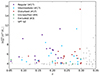 |
Fig. 1. Studied sample (colored points) and entire SPT catalog (gray points, Bocquet et al. 2019). Gray points within the redshift-mass selection area did not meet the S/N or footprint constraints. Crosses indicate galaxy clusters that were subsequently removed from our sample. |
The raw Compton-y map of each cluster was extracted from the Sanson-Flamsteed projection minimum-variance Compton-y maps based on both SPT and Planck data (Bleem et al. 2022). Their radial profiles were computed in circular annuli with a width of 75 arcsec, which corresponds to the beam’s full width at half maximum (FWHM), accounting for field boundaries and after flagging other sources and regions of lower quality. The chosen width ensures that the data covariance between radial bins is negligible. We adopted as centers the coordinates derived by Bocquet et al. (2019) and the point spread function (PSF) and transfer function provided with the Compton maps (Bleem et al. 2022). To estimate the errors of the profiles, we measured the scatter across profiles computed from random centers placed around each cluster. Radial profiles were extracted up to r ∼ 17.5 arcmin. At a round number close to the median redshift, z = 0.2, the data are sampling the pressure profile with a 250 kpc scale FWHM, a scale much smaller than the cluster diameter at Δ = 500, typically 3 Mpc1.
We cross-matched our sample with the eROSITA catalog from the eRASS1 survey (Bulbul et al. 2024) to classify the clusters according to their morphological properties. We adopted the disturbance indicator Dcomb defined by Sanders et al. (2025), which combines information on the shape and concentration of the cluster. Data were available for 51 out of the 55 galaxy clusters in our analysis. As is shown in Fig. 1, we divided these clusters into three tertiles: Dcomb < 0.02 (dubbed regular), 0.02 < Dcomb < 0.4 (intermediate) and Dcomb > 0.4 (disturbed). Their morphological indicator is a combination of indices, not all of which account for the PSF, data noise, and redshift dependence, and which tend to be weighted toward the bright central regions of clusters, resulting in biases in the presence of a cool-core (Sanders et al. 2025). Figure 1 indicates that clusters classified as disturbed tend to have higher redshifts than those classified as relaxed.
2.2. Pressure profile modelization
To model the pressure profile of galaxy clusters, we adopted restricted cubic splines (Durrleman & Simon 1989). These functions combine the flexibility of cubic interpolation between the innermost and outermost knots with linear regression at both extremities, avoiding undesired twists in the pressure profile at radii that are essentially unconstrained by data, namely well inside the beam FWHM and at radii where the S/N is vanishing.
The equation for a restricted cubic spline model with K knots is
 (1)
(1)
where
![Mathematical equation: $$ \begin{aligned} f(r,R_j) = \,&\bigg [ \big (r - R_j\big )^3_+ - \frac{R_K - R_j}{R_K - R_{K-1}} \big (r - R_{K-1}\big )^3_+ + \nonumber \\&+ \frac{R_{K-1} - R_j}{R_K - R_{K-1}} \big (r - R_K\big )^3_+ \bigg ], \end{aligned} $$](/articles/aa/full_html/2025/10/aa55522-25/aa55522-25-eq3.gif) (2)
(2)
where (R1, …, RK) are the knots and the “+” notation indicates
 (3)
(3)
Splines were computed in log-log space to avoid unphysical negative values for either radii or pressures. To ensure a finite integral and to distinguish between a radially flat background and a radially flat cluster signal, we set an upper limit for the slope value beyond the largest knot, as done in previous works (Romero et al. 2018; Andreon et al. 2021). In our analysis, we constrained this slope to be negative, which is less restrictive than in previous works.
Since clusters have different masses and sizes, we used the scaled pressure profiles, p(x), defined in Arnaud et al. (2010) as follows:
![Mathematical equation: $$ \begin{aligned} p(x) = \frac{P(r)}{P_{500}}\left[\frac{M_{500}}{3\times 10^{14}M_\odot }\right]^{\alpha _P+\alpha ^{\prime }_P(x)}, \end{aligned} $$](/articles/aa/full_html/2025/10/aa55522-25/aa55522-25-eq5.gif) (4)
(4)
where x = r/r500, αP ≃ 0.12, and
 (5)
(5)
P500, the characteristic pressure, was computed according to the following equation:
![Mathematical equation: $$ \begin{aligned} P_{500}=\frac{3}{8\pi }\left[\frac{500\,G^{-1/4}H(z)^2}{2}\right]^{4/3}\frac{\mu }{\mu _e}\,f_B\,M_{500}^{2/3}, \end{aligned} $$](/articles/aa/full_html/2025/10/aa55522-25/aa55522-25-eq7.gif) (6)
(6)
where  is the Hubble parameter at a given redshift, G is the gravitational constant, fB = ΩB/ΩM = 0.175 is the mean baryon fraction in the Universe, μ = 0.59 is the mean molecular weight, and μe = 1.14 is the mean molecular weight per free electrons.
2.3. Likelihood function computation for the i-th cluster
The three-dimensional pressure profile of Sect. 2.2 was numerically integrated along the line of sight through an Abel transform to obtain a two-dimensional map of the Compton-y parameter, which was then convolved to account for the beam and transfer function. Finally, the radial profile was extracted from the filtered Compton-y parameter map, converted to the surface brightness unit, and compared to the observed data within a Bayesian framework, yielding the pressure profile parameters and their associated errors. We added a pedestal parameter to the surface brightness profile to account for a nonzero background level, adopting a Gaussian distribution centered on 0 with σ = 10−6 as prior. For all these operations, we used PreProFit, as detailed in Castagna & Andreon (2019). The updated code, which allows users to adopt a restricted cubic spline model, as well as a generalized Navarro, Frenk & White (gNFW) profile (Nagai et al. 2007), a piecewise power law, or a cubic spline model, is publicly available on GitHub2.
2.4. Mass definition
The  values in the SPT catalog (Bocquet et al. 2019) are unreliable because the derived
  values are, in some cases, manifestly too large or too small compared to the angular size of the cluster, regardless of whether these values are corrected by the 0.8 factor proposed in Tarrío et al. (2019), as illustrated below. We therefore estimated the cluster’s M500 mass from its SZ flux, Y500, using
![Mathematical equation: $$ \begin{aligned} E^{-2/3}(z) \left[ \frac{D_A^2 Y_{500}}{10^{-4} \mathrm{Mpc} ^2} \right] = 10^{-0.19} \left[ \frac{M_{500}}{6\times 10^{14} M_\odot } \right]^{1.79}, \end{aligned} $$](/articles/aa/full_html/2025/10/aa55522-25/aa55522-25-eq11.gif) (7)
(7)
where E(z) = H(z)/H0 is the dimensionless Hubble parameter and DA is the angular diameter distance (Planck Collaboration XX 2014), as illustrated in Fig. 2 for two clusters. We adopted r500 values derived from the fit pressure profile model rather than from the data because the model enforces regularity in the case of noisy data (e.g., see left panel) and does not harm high-quality data (e.g., see right panel). Y500 and M500 values for each cluster are reported in Table 2.
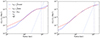 |
Fig. 2. Derivation of r500 for two galaxy clusters, SPT-CLJ0051-4834 (left panel) and SPT-CLJ0328-5541 (right panel), shown as examples. Integrating the model ensures regularity in the case of noisy data (left panel) and does not affect high-quality data (right panel). |
Figure 3 compares our r500 values with the  values from the Planck catalog (Planck Collaboration XXVII 2016) in the left panel for the 38 objects in common, and with the
  values from the SPT catalog (Bocquet et al. 2019) in the right panel for the entire sample. The
  values are derived from a measurement at 5r500, scaled down by an amount fixed by the Planck team assuming the pressure profile of Arnaud et al. (2010). The
  values, on the other hand, are inferred in Bocquet et al. (2019) from the cluster detection probability. Our r500 values are in good agreement with Planck values, with most of them tightly aligned along the
  relation (dotted blue line). On the other hand, we observe no agreement between our r500 and
  , which justifies the decision to recompute these values through Y500. In particular, the
  values show a large scatter because the spatial Compton-y signal assumed an overly constrained profile model, as earlier mentioned and detailed in Sect. 3.1.
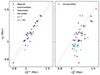 |
Fig. 3. Comparison of our estimates of r500 (y axis) with Planck for the 38 clusters in common (left panel) and with SPT for the entire sample (right panel). Our r500 values are strongly correlated with the Planck ones, while a larger scatter is observed when compared with SPT. No morphology-dependent trend is observed. |
2.5. Hierarchical model for the population of clusters
To model the variety of pressure profiles of clusters with the same mass, we used a two-level BHM. This approach allows us to estimate the average pressure profile and the intrinsic scatter for a population of galaxy clusters. The top level models the population, while the bottom level models the individual clusters. The population-averaged pressure profile is modeled (nonparametrically) with a restricted cubic spline with nk knots. At each knot, the scatter of the individual profiles from the average is modeled with a Student’s t distribution with 10 degrees of freedom. We preferred a Student’s t over a Gaussian because it is less sensitive to outliers (e.g., Andreon & Hurn 2010). However, we also performed an additional analysis using a Gaussian distribution for the scatter, which yielded very similar results.
In detail, at the k-th knot of i-th cluster, the individual pressures lgPk, i can scatter around the population-averaged pressure lgPk as
 (8)
(8)
The coefficient in front of the scale parameter ensures that Var(tν) = σint, k2, allowing us to correctly interpret the σint, k parameters as estimates of the intrinsic scatter. lgP is a shorthand for log10(p(x)).
Our prior of the population-averaged pressure profile at the k-th knot is a Gaussian with a large σ (0.5 dex) centered on the universal pressure profile (UPP, Arnaud et al. 2010):
 (9)
(9)
The prior on the scatter is a uniform distribution over a wide range (from 0 to 1 dex), largely encompassing all plausible values:
 (10)
(10)
Our model has (2 × nk) parameters describing the population, namely the average pressures at the nk knots and the dispersions around them, plus (nk+1) parameters per cluster, namely the individual pressures at the nk knots and the pedestal parameter.
2.6. Model and MCMC settings
Throughout our analyses, we set the number of knots to nk = 5 and placed them at fixed locations: [0.1,0.4,0.7,1,1.3] × r500. With this radial scaling, we assume that the scatter is a function of r500, as in previous works (e.g., Ghirardini et al. 2019), rather than, for example, radii that do not scale with mass. The spacing of the knots was chosen to be larger than the width of the radial binning to avoid strong covariances between radially adjacent estimates, while the innermost radius was set at 30 arcsec in order to prevent us from undersampling the PSF FWHM. The MCMC estimations were performed using the PyMC Python package3 (Patil et al. 2010) with the default sampling methods. We ran 8000 iterations with 24 walkers, discarding the first half iterations as a burn-in period. We then compared the posterior distributions of all walkers and removed some walkers that had not fully converged.
3. Results
3.1. Exploratory analysis and cluster characterization
We started by fitting each individual galaxy cluster independently of the other ones using a standard Bayesian analysis with uniform priors for the pressure values to assess whether our chosen model of the pressure profile is adequate for the used data. Figure 4 shows the distribution of the reduced chi-square χν = 92 for this exploratory analysis (red histogram), compared with the analogous measures for the subsequent population analysis (blue histogram). This goodness-of-fit evaluation is performed by comparing the median surface brightness profile, obtained by computing the median value across all posterior profiles at each radial bin, with the observed data, and therefore does not provide the minimal χν2. All individual fits, except one, show acceptable χν2 values, suggesting that the adopted spline with five knots is sufficiently flexible to describe the pressure profiles of the studied clusters given the data quality. The object with a large χν2 is SPT-CLJ0405-4916, and its value is due to an oscillating background level due to contamination. For this reason, SPT-CLJ0405-4916 has been removed from the sample. The results of the population fit show acceptable χν2 values, suggesting that the population analysis presented in the following section appropriately models all clusters in the sample.
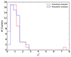 |
Fig. 4. Distribution of the reduced chi-square χν = 92 of the 58 individual fits and the population fit of 55 clusters. The red outlier with χν2 > 7 is SPT-CLJ0405-4916, which is characterized by a highly oscillating surface brightness distribution in its outermost region, while our background model, the pedestal, is a constant. For this reason, we excluded it from the population analysis. |
Figure 5 shows the distribution of the number of resolution elements for all 58 clusters, defined as the ratio between θ500, namely the characteristic radius r500 in angular units, and the beam’s half width at half maximum (HWHM), which in our case equals 0.625 arcmin. Because of our selection based on mass and redshift, all clusters have θ500/HWHM > 5, i.e., are well resolved, making the assumption used in Bocquet et al. (2019) to derive their (SZ) mass invalid for our sample and justifying our redetermination of it. Two objects (SPT-CLJ2012-5649 and SPT-CLJ0431-6126), with θ500/HWHM > 30, are so extended that we chose to exclude them from our sample for computational reasons: including them would considerably increase the computation time of the hierarchical model. Figure 6 shows how our selection resulted in a sample of more resolved clusters compared to other works in the literature that analyzed samples of clusters using SZ data (Sayers et al. 2016; Pointecouteau et al. 2021; Melin & Pratt 2023).
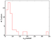 |
Fig. 5. Distribution of the number of resolution elements, θ500/HWHM, across the initial sample of 58 objects. Because of our careful sample selection in mass and redshift, all clusters have θ500/HWHM > 5, i.e., are well resolved. The two clusters with θ500/HWHM > 30 are excluded from later analyses because of the high computational time required to include them in the hierarchical model. |
Figure 7 compares our integrated Compton parameters within 0.75 arcmin,  , with the values published by Bleem et al. (2015) for the sample of 58 clusters. The determination of Bleem et al. (2015) assumes that the cluster profile follows a β-model, and uses shallower data. Apart from the fact that their values are larger by approximately 23%, likely due to the overly constrained model adopted, there is general agreement between the two determinations. Our values are reported in Table 2.
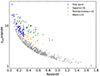 |
Fig. 6. Resolution of galaxy clusters in our sample and in works that analyze galaxy clusters using only SZ instruments (Sayers et al. 2016; Pointecouteau et al. 2021; Melin & Pratt 2023). Compared to other studies, our selection focuses on well-resolved clusters. |
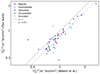 |
Fig. 7. Integrated Compton parameter |

3.2. Population analysis
The population analysis simultaneously fits the population-averaged pressure profile and the 55 individual pressureprofiles of the galaxy clusters. Figure 8 shows the individual surface brightness profiles from the population analysis for two clusters, taken as examples, together with the observed data and the corresponding profiles from the individual analyses of the previous section. The plot highlights an acceptable fit of the hierarchical model for the two selected clusters, quantified, as mentioned, in Fig. 4 for all 55 clusters, demonstrating that the chosen model is appropriate for the data used. The two chosen clusters undergo a change in concavity in the pressure profile around the third interpolation knot (see Fig. 9), an aspect that our model accommodates, unlike other pressure profile parametrizations.
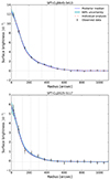 |
Fig. 8. Surface brightness profiles of two clusters, taken from the population analysis. Vertical dotted gray lines show the placement of the knots, whereas the horizontal one indicates the estimated pedestal level. The plots highlight that our radial profile parametrization is adequate for these two clusters. Figure 4 quantifies the fit for the entire sample. |
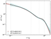 |
Fig. 9. Pressure profiles of the two clusters in Fig. 8. Vertical dotted gray lines show the placement of the knots. The plot highlights a marked change in concavity around the third interpolation knot. |
Figure A.1 compares our individual cluster pressure profile estimates with derivations by other authors who fit nonparametric models on SZ data (Ghirardini et al. 2019; Sayers et al. 2023), for the four objects for which data are available. Our pressure profiles are generally consistent with the results from other studies.
Trace plots and marginal probability distributions for the population parameters (color-coded by walker) are shown in Fig. B.1. Table 1 lists the population parameter estimates (the population-averaged pressures lgPk and the intrinsic scatters σint, k), while Table 2 lists the individual pressure parameter estimates lgPk, i. These individual estimates are more accurate than those obtained from fitting each cluster independently, as the joint hierarchical model leverages the population-level posteriors as informative priors for the individual lgPk, i.
Population-averaged pressure and intrinsic scatter values for the entire studied sample and for the morphological classes.
Sample of galaxy clusters and estimated parameters in the population analysis. The full table is available at CDS.
Figure 10 shows the joint and marginal probability distributions for the population parameters: the population-averaged pressure values (top panel) and the intrinsic scatters (bottom panel) at the five radii [0.1,0.4,0.7,1,1.3] × r500. The Bayesian approach inherently accounts for the covariance among parameters. However, this covariance is weak for these parameters due to our choice of the modeling function (a restricted cubic spline) and the spacing of the knots. Figure 11 shows the correlation matrix for all 340 fit parameters, where each value ρi, j represents the correlation between the parameter pair (θi, θj). While most parameters are nearly uncorrelated, two pairs stand out. The pressure at the outermost radius is strongly anticovariant with the pedestal, indicating that the data cannot distinguish a flat cluster profile from a flat background, despite our prior on the outer slope of the profile. Additionally, the pressures at the first two knots are anticorrelated, as the data largely constrain a quantity near their sum because of PSF effects. As is shown in Sect. 4.1, our modelization for the pressure is preferable to using a gNFW profile. Since the prior distributions are nearly uniform in the range where the posteriors are nonzero (Fig. 10), their impact on estimating the population parameters is minimal. Even the prior constraint to force a negative outer slope (beyond 1.3r500) has a negligible impact on the results: the 2σ upper limit of the slopes is < 0 for 51 out of 55 clusters and the population-averaged mean slope is −5.38 ± 0.65. We also performed an alternative fit, modeling the inverse of the intrinsic scatter with a Gamma prior distribution, and obtained similar results.
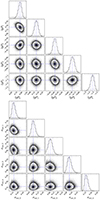 |
Fig. 10. Joint and marginal posterior distributions for the population-averaged pressure parameters lgPk (top panel) and intrinsic scatters σint, k (bottom panel) at the five radii (interpolation knots). Dashed blue lines represent the median values. In the diagonal panels, vertical dotted blue lines indicate the 68% uncertainty interval, while dashed black lines represent the adopted prior. All parameters show little correlation, due to our choice of the radial profile modelization and the knots spacing. Prior distributions have a negligible impact on the posterior distributions. |
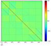 |
Fig. 11. Correlation matrix for all 340 fit parameters. Most parameters show little covariance, except between the pressures of the two inner knots and between the pressures at the last knot and the pedestal parameters (see text for details). These low correlations contrast with those observed in the fit using a gNFW model (see Fig. 18). |
Figure 12 shows the main result of our work encompassing estimates from both levels of the hierarchical model. The top panel shows the population-averaged pressure profile (solid blue line), its 68% uncertainty (blue shaded area), the 68% intrinsic scatter around it (error bars), and the individual cluster estimates from the population analysis (dashed gray lines). We emphasize that, with noisy data, we expect more than 68% of the individual posterior median profiles to lie within the 1σint interval. This occurs because the prior on the population parameters attracts the individual posterior parameters toward the mean, as in the SN fit shown by Andreon (2012). The central panel shows the radial distribution of the intrinsic scatter, estimated at the five knots. The dispersion is minimal at intermediate radii (second and third knots), which confirms and reinforces that the intermediate cluster regions are the most regular (Arnaud et al. 2010). At an attentive inspection, at least some individual profiles (e.g., SPT-CLJ0645-5413, SPT-CLJ2025-5117, SPT-CLJ0225-4327) undergo a change in concavity between the third and fourth knot (as is shown in Fig. 9). The fraction of profiles with a change in concavity depends on the threshold used to classify objects as members of the class. This change in concavity is not allowed with a gNFW profile, and as a consequence, has never been seen in previous works using this radial model. The inspection of the data (e.g., Fig. 8) confirms that the model captures the data behavior. Inspection of the XMM X-ray data for the clusters exhibiting a change in concavity does not reveal any obvious distinguishing features compared to the rest of the sample. The bottom panel shows the number of clusters that contributed to the derivation of the population-averaged pressure profile at different radii, noting that for some clusters the innermost radial bin (30 arcsec) is larger than the innermost interpolation knot. Around half of the clusters in the sample contribute to the determination of the intrinsic scatter at the innermost interpolation knot, r = 0.1r500.
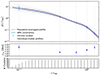 |
Fig. 12. Pressure profiles (top panel) and intrinsic scatter (top and central panels) of our population analysis. The scatter is minimal at 0.4r500 ≤ r ≤ 0.7r500. The bottom panel shows the number of objects contributing at each radius. |
Figure 13 shows the pressure estimates of individual clusters lgPk, i (points with error bars) together with the population-averaged pressure values lgPk (solid lines), their errors (shaded areas) and intrinsic scatters (dotted lines). This visualization highlights that we did not detect any cluster with outlier pressure parameters, despite allowing for such outliers by using a Student-t distribution to model the scatter. Only two individual pressure estimates lie beyond the 2σint threshold: one at the second and one at the fifth knot. Figure 14 shows the pressure estimates of individual clusters as a function of P500, suggesting that there is no discernible trend of dependence on it.To formally evaluate potential dependencies of the population parameters on P500 and redshift, we extended our baseline fitting model to include these effects. Specifically, we added to Eq. 8, in turn, γPlog(P500, i/P500, med) and γzlog((1 + zi)/(1 + zmed)), where P500, med and zmed are the sample medians. We adopted a Student’s t distribution with one degree of freedom (equivalent to a uniform prior on the angle) for each additional parameter γ. To assess the preference for the extended model over the baseline one, we computed the Bayes factor using the Savage-Dickey density ratio (Dickey 1971), as the models are nested. As is shown in Fig. 15, the data favor the absence of a dependence on P500, with a Bayes factor of 16.5, indicating moderate to strong evidence and supporting our decision not to include this term in the model. Instead, the comparison yields inconclusive evidence of redshift dependence, with the relative odds between the models being comparable.
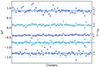 |
Fig. 13. Individual pressure parameters lgPk, i (points with error bars) at the five knots (marked on the right y axis). Horizontal lines represent the population-averaged pressure estimates lgPk (solid lines) with their errors (shaded areas), and intrinsic scatter estimates (dotted lines). |
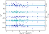 |
Fig. 14. Individual pressure parameters lgPk, i (points with error bars) at the five knots (marked on the right y axis) as a function of the cluster’s P500. Horizontal lines represent the population-averaged pressure estimates lgPk (solid lines) with their errors (shaded areas), and intrinsic scatter estimates (dotted lines). |
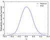 |
Fig. 15. Probability density function for the posterior and prior distributions of γP. A Bayes factor of 16.5 is moderately in favor of no dependence on P500. |
Figure 16 shows the population-averaged pressure profiles of the regular and disturbed clusters separately. These profiles were derived from joint fits of clusters belonging to these classes, as done for the entire sample, and the estimated parameters are reported in Table 1. Regular clusters exhibit a more peaked profile at the center (indicative of cool cores) compared to disturbed clusters, and show lower intrinsic scatter beyond the innermost knot, indicating that part of the pressure profile heterogeneity in the full sample is related to cluster morphology. The pressure profile and scatters of clusters morphologically classified as intermediate lie between them (not shown in the plot to avoid crowding). Since the disturbed clusters subset includes objects with a disturbance indicator spanning a large range (0.4 < Dcomb ≤ 1), we also performed an additional comparison by splitting this group into two further subsets, using Dcomb = 0.75 as the threshold. Even in this case, no significant differences were found.
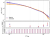 |
Fig. 16. Pressure profiles (top panel) and intrinsic scatter (top and central panels) of regular and disturbed clusters. Error bars and shading as in Fig. 12. Points are slightly horizontally offset for clarity. Regular clusters seem to show a lower scatter at r ≥ 0.4r500 and a more peaked profile at the center. The bottom panel shows the number of objects contributing at each radius. |
The top panel of Fig. 17 compares our population-averaged pressure profile with results from other works. Our profile exhibits a pressure deficit of approximately 12 ± 3% compared to the UPP (Arnaud et al. 2010, solid black line). The median absolute fractional difference between our profile and the 12 ± 3%-reduced UPP (dashed black line) is only ∼6%, indicating that deviations are minimal at the resolution offered by our data (250 kpc FWHM). Within r500, our profile agrees well with that of the low-z sample from Sayers et al. (2023, green points). The profile of Pointecouteau et al. (2021, orange line) shows an even more marked pressure deficit than ours within 0.6r500, while that of Ghirardini et al. (2019, red lines) lies systematically above all others. Beyond r500, our profile declines more steeply than those in these three works, which mostly rely on Planck at large radii.
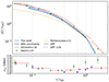 |
Fig. 17. Pressure profiles (top panel) and intrinsic scatters (bottom panel) for our sample and literature works, with literature errors omitted from the top panel for clarity. Within r500, our profile is ∼12% lower than the UPP, close to what is needed to remove the tension in cosmological parameters derived from CMB and Planck SZ cluster counts (Ruppin et al. 2019). The steep decline of our pressure profile beyond r500 is consistent with the deficit reported by Anbajagane et al. (2022), interpreted as a shock-induced thermal nonequilibrium between electrons and ions. Regarding the scatter, the three radial profiles are consistent up to 0.4r500. Beyond this radius, Sayers et al. (2023) report the highest scatter, while our analysis yields the lowest. |
The observed ∼12% pressure deficit relative to the UPP is consistent with the ∼15% reduction proposed by Ruppin et al. (2019) to alleviate the tension between cosmological parameters derived from the CMB and Planck SZ cluster counts. It is also in agreement with the revised UPP from He et al. (2021), which assumes a mass bias derived from simulations and whose predicted power spectrum at multipoles 100 < l < 1000 approximately matches the value observed by Planck, whereas the original UPP overestimated the signal by up to 50%. The steep decline of our pressure profile beyond r500 is consistent with the deficit reported by Anbajagane et al. (2022), interpreted as a shock-induced thermal nonequilibrium between electrons and ions. This lower pressure and steeper profile beyond r500 is also in line with the conditions required to reconcile the observed and predicted angular power spectrum of the thermal SZ effect in the work of Ramos-Ceja et al. (2015).
As was previously noted, our pressure values at the outermost knot are correlated with the pedestal estimates. Thiscorrelation does not significantly affect the slope at large radii: removing the pedestal from the model and refitting the data yields a similar population-averaged profile. Nevertheless, distinguishing a weak, approximately constant signal from the background remains inherently challenging, both in our work and in other works, regardless of whether the pedestal is included in the model.
Sample selection is unlikely to explain the differences among the pressure profiles obtained by different works. Pointecouteau et al. (2021) and Ghirardini et al. (2019) analyzed SZ-selected samples, such as ours, yet found discrepant results in opposite directions, with the Ghirardini et al. (2019) profile lying above the UPP, potentially increasing the cosmological tension. Arnaud et al. (2010) and Sayers et al. (2023)studied X-ray-selected samples – based on XMM and Chandra data, respectively – with Sayers et al. (2023) also incorporating high-resolution SZ observations. Pressure estimatesincluding X-ray data are less direct due to the assumption of clumpiness (Eckert et al. 2015) and differences between mass-weighted and X-ray temperatures (Vikhlinin et al. 2006). Additionally, a long-standing issue with absolute X-ray calibration, particularly between Chandra and XMM (Schellenberger et al. 2015), may contribute to the observed differences when not considered. Since all of these works probe comparable regions of the redshift-P500 plane, and we detect no dependence of the pressure parameters on redshift or P500 (Fig. 15), the observed differences between profiles cannot be attributed to variations in either of these parameters.
The bottom panel of Fig. 17 compares our estimate of the intrinsic scatter with those of Ghirardini et al. (2019) and Sayers et al. (2023), both of which adopt, as our work does, a nonparametric model for the pressure profile. The three radial profiles of intrinsic scatter are consistent up to 0.4r500. Beyond this radius, Sayers et al. (2023) report the highest scatter, while our analysis yields the lowest. Although SZ-selected samples are expected to encompass more heterogeneous populations of clusters than X-ray-selected samples (Planck Collaboration IX 2011; Andreon et al. 2016; Rossetti et al. 2017), this expectation is not reflected in the intrinsic scatter estimates: the scatter in the X-ray-selected sample of Sayers et al. (2023) is systematically larger beyond 0.6r500 than in the SZ-selected samples of our work and Ghirardini et al. (2019).
3.3. Sensitivity analyses
Our analysis excludes three clusters within the redshift range, potentially introducing some incompleteness into the sample. Although formally incomplete, the sample remains representative because these clusters were removed for reasons not related to their Compton-y signal, making it a random sampling of a complete cluster, and therefore their removal should not affect our results. Nevertheless, we assess the impact of this random incompleteness by slightly narrowing the redshift range and re-fitting all 49 clusters within the interval 0.08 < z < 0.29, a range in which no clusters were excluded. The resulting posterior means and uncertainties of the population-averaged pressure parameters at the five knots, along with three of the five intrinsic scatter parameters, remain unchanged. The posterior means of the remaining two intrinsic scatters differ byapproximately 1σ.
Our analysis includes clusters with Compton-y S/N as low as 5, consistent with other studies that also adopt similar or even lower thresholds (e.g., Pointecouteau et al. 2021). To assess the robustness of our results to the S/N cut, we repeated the analysis using only the 33 clusters within our sample with S/N > 6. The results are very similar to those obtained from the full sample, with a mean absolute standardized difference of 0.56 between the population parameters of the two models.
In our analysis, we adopted a specific Y-M scaling relation (Eq. 7). Preliminary tests using an alternative scaling relation and a reduced sample, chosen to limit computational cost, indicate that the resulting mean pressure profile is sensitive to the choice of scaling relation. The observed variation exceeds our current uncertainty estimates, due to the precision achieved by our large sample. As with all analyses, our results are conditional on the underlying assumptions, which in our analysis and similar ones include the adopted cosmology and the Y-M scaling relation. A more comprehensive investigation, possibly including a simultaneous fit of the scaling parameters, is deferred to future work.
4. Discussion and conclusions
4.1. Astrostatistics considerations
Our approach sets a new standard compared to previous analyses. First, we introduce the restricted cubic spline interpolation model for the pressure profile, which offers several advantages. It improves on the cubic spline interpolation model (Andreon et al. 2021, 2023) as it avoids undesired twists in the pressure profile at radii that are essentially unconstrained by the data. It does not show the irregular uncertainties (larger near the knots and smaller at the center of the interpolation intervals) observed with the power-law interpolation model adopted, for example, by Romero et al. (2018) and Kéruzoré et al. (2023). By not assuming a parametric form for individual cluster and population-averaged profiles, we do not impose a model on nature, unlike the gNFW radial profile. As a result, the restricted cubic spline model can flexibly capture changes in the concavity of the pressure profile, unlike more constraining parametrizations such as the gNFW or power-law models. Second, our choice of profile parametrization makes the parameters easier to interpret and breaks the strong covariance present, for example, in fits that assume a gNFW model. Figure 18 shows the correlation matrix for the analysis performed using a gNFW parametrization (Nagai et al. 2007) instead of restricted cubic splines. The differences compared to the correlation matrix in Fig. 11 are substantial. Third, by fitting the population and the individual clusters simultaneously in a BHM, we avoid the inconsistency of widespread two-step analyses, which first assume a uniform prior for a parameter (e.g., the profile normalization) during the individual fits and subsequently impose a normal distribution on it. Fourth, by adopting a Student-t distribution, we account for outliers, i.e., clusters with unusual pressure profiles, which are automatically identified and downweighted in the computation of the average profile. This approach eliminates the need for manual examination and the use of arbitrary criteria (such as a 3σ clipping, which may be based on a preliminary computed σ), as was previously done (e.g., Ghirardini et al. 2019). Fifth, rather than blindly assuming a model for the individual pressure profile, we critically assess its validity by checking how well it fits the data (see Fig. 4 and discussion therein). Similarly, rather than blindly assuming no evolution and no P500 dependency of population parameters, we use the Bayes factor to choose whether to include them in the model. Finally, when a parameter is unconstrained, rather than arbitrarily fixing its value and excluding all other possibilities, including those differing negligibly, our joint fit marginalizes over the prior distribution. When a parameter is unconstrained for a cluster, the joint fit uses the information from the whole sample as an effective prior, improving its value and uncertainty.
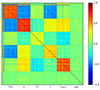 |
Fig. 18. Correlation matrix for all 340 fit parameters in an analysis performed assuming a gNFW model for the pressure profile. Many parameters show a strong level of covariance, much higher than with our pressure parametrization, whose correlation matrix is shown in Fig. 11. |
From a computational perspective, this process is highly time-consuming due to the simultaneous fitting of 340 parameters. However, PyMC is particularly effective for modeling complex dependencies in hierarchical Bayesian frameworks. It supports multidimensional parameters in hierarchical models by allowing group-level distributions to define structured dependencies across multiple levels. PyMC also enables vectorized priors through the “shape” argument, ensuring computational efficiency and automatic sharing of statistical strength across groups.
4.2. Astronomical considerations
We fit our model on the largest non-stacked sample of individual cluster radial profiles (55 objects), computing the population-averaged profile and the intrinsic scatter around it, as described by the parameters in Table 1. We also derived the parameters of the individual pressure profiles (see Table 2) by leveraging information from clusters with well-determined profiles. By applying appropriate selection criteria in mass and redshift, we avoid attempting to measure the pressure profile of clusters that are unresolved with the data (see Fig. 6). Following the identification of inconsistencies in some M500 estimates, we rederived all normalizations under weaker assumptions. We identified some clusters with radial pressure profiles that exhibit a change in concavity. Although the model allows for outliers, none are detected in the pressure values of individual clusters. Compared to Arnaud et al. (2010), our determination extends to radii 1.4x larger and includes more objects in each morphologically defined class (17 vs. 10 or 11). Compared to Ghirardini et al. (2019), whose scatter estimates are based on just four and eight clusters per class and thus considered potentially unreliable, we can split our sample into morphological classes with a significantly larger number of objects per class. Despite the unprecedented precision enabled by the largest sample of resolved clusters and the flexibility offered by our spline-based radial profile, the population-averaged profile is close to the UPP within r500 (Fig. 12), indicating that deviations are minimal at the resolution offered by our data (250 kpc FWHM). Our profile is even more closely aligned with the ∼15% decreased version of the UPP proposed by Ruppin et al. (2019) to alleviate tensions between cosmological parameters as derived from the CMB and Planck SZ cluster counts. The steep decline of our pressure profile beyond r500 is consistent with the deficit reported by Anbajagane et al. (2022), interpreted as a shock-induced thermal nonequilibrium between electrons and ions. At large radii, specifically around r = 1.4r500, distinguishing a weak, approximately constant signal from the background is inherently challenging. As a result, pressure measurements and slope estimates at these radii should be interpreted with caution. This is true regardless of whether the background level along the cluster line of sight is allowed to deviate from that measured in a reference region (as done in our analysis) or is assumed to be identically zero (as in several other studies). The dependencies on redshift and P500 are also weak and not appreciable in our sample. The intrinsic scatter is minimal at intermediate radii, approximately between 0.4r500 and 0.7r500, and is lower than that determined by Sayers et al. (2023), who use X-ray-selected samples. This result is especially notable given that our sample is SZ-selected, and thus expected to encompass a more heterogeneous population of clusters. Splitting the sample according to morphological types gives similar pressure profiles for the two classes, with some evidence that morphologically regular clusters show a lower intrinsic scatter and a more peaked profile at the center than disturbed clusters. Cluster morphology is a component contributing to the heterogeneity of pressure profiles within the analyzed sample.
4.3. Limitations and future developments
Samples without any SZ-based selection do not require corrections for a never-applied SZ selection. Therefore, our approach can be directly applied - without modification - to samples selected, for example, through gravitational lensing, such as those detected by Oguri et al. (2021) and studied by Andreon & Radovich (2025), or those to be released in the upcoming Data Release 1 of the Euclid survey (Euclid Collaboration: Mellier et al. 2025). However, for samples similar to the one analyzed here, as well as in most previous works, the selection function has to be modeled and incorporated into the fit. Therefore, the conclusions derived from our analysis apply only to the studied sample or to samples selected in similar ways, rather than to the entire population of clusters. As a consequence, the heterogeneity observed in our sample is an underestimate of the actual heterogeneity. Indeed, there are already known examples of clusters whose pressure profile is manifestly different from those derived from ICM-selected samples (Andreon et al. 2019, 2021, 2023). Neglecting the selection function was a necessary simplification in this first step; modeling it represents a natural direction for future work. Additional possible developments include the use of multiwavelength data, such as combining SZ measurements with X-ray and weak lensing observations, which would further enhance the robustness of our analysis by integrating complementary information and providing a more complete picture of clusterproperties.
5. Conclusions
We developed a Bayesian hierarchical model that simultaneously and coherently fits both the parameters of individual clusters and those of the population from which they are drawn. We introduced a highly flexible, low-covariance parametrization of the pressure profile using restricted cubic splines, which provide a simple and intuitive interpretation of the parameters. To account for outliers, we modeled the scatter with a Student-t distribution and assessed the appropriateness of the fit radial profile against the data. We also applied the beam and transfer function corrections, as is required for SZ data. We used the Bayes factor to choose between possible modelizations. Our method was applied to the largest non-stacked sample of clusters with resolved pressure profiles, extracted from SPT+Planck Compton-y maps. This sample consists of 55 clusters, large enough to be divided into three morphological classes based on eROSITA data. Computations are feasible within a few days on a modern (2024) personal computer. The shape of the population-averaged pressure profile, at our 250 kpc resolution, closely resembles the universal pressure profile, despite the flexibility of our model for accommodating alternative shapes, with a ∼12% lower normalization, close to what is needed to alleviate the tension between cosmological parameters derived from the CMB and Planck SZ cluster counts (Ruppin et al. 2019). At the largest radii, our profile is steeper than other works, but in agreement with the pressure deficit observed by Anbajagane et al. (2022), interpreted as a shock-induced thermal nonequilibrium between electrons and ions. A lower pressure profile that steepens at large radii is also required to reconcile the predicted and observed thermal SZ power spectrum. The estimate of the intrinsic scatter is consistent with or lower than previous estimates, although our SZ-selected sample is expected to include more heterogeneous clusters than the X-ray-selected samples used for comparison. Using our flexible pressure model, we identified a few clusters whose radial pressure profiles display a change in concavity. Although the model allows for outliers, none are detected in the pressure values of individual clusters. When splitting the sample by morphological type, we found that the profiles of the two extreme tertiles are remarkably similar, with some evidence suggesting that morphologically regular clusters exhibit lower intrinsic scatter and more centrally peaked profiles compared to disturbed clusters. Therefore, morphology is a key contributor to the observed heterogeneity in pressure profiles.
Data availability
Full Table 2 is available at the CDS via https://cdsarc.cds.unistra.fr/viz-bin/cat/J/A+A/702/A105
Acknowledgments
We thank Merrilee Hurn for helpful statistical advice, Om Sharan Salafia for fruitful discussion, and Jack Sayers for useful comments. FC and SA acknowledge INAF grant “Characterizing the newly discovered clusters of low surface brightness” and PRIN-MIUR grant 20228B938N “Mass and selection biases of galaxy clusters: a multi-probe approach”, the latter funded by the European Union Next generation EU, Mission 4 Component 1 CUP C53D2300092 0006.
References
- Anbajagane, D., Chang, C., Jain, B., et al. 2022, MNRAS, 514, 1645 [NASA ADS] [CrossRef] [Google Scholar]
- Andreon, S. 2012, in Astrostatistical Challenges for the New Astronomy, ed. J. M. Hilbe (Springer), 41 [Google Scholar]
- Andreon, S., & Hurn, M. A. 2010, MNRAS, 404, 1922 [NASA ADS] [Google Scholar]
- Andreon, S., & Radovich, M. 2025, ApJ, 985, 78 [Google Scholar]
- Andreon, S., & Weaver, B. 2015, Bayesian Methods for the Physical Sciences. Learning from Examples in Astronomy and Physics, 4 (Springer) [Google Scholar]
- Andreon, S., Serra, A. L., Moretti, A., & Trinchieri, G. 2016, A&A, 585, A147 [NASA ADS] [CrossRef] [EDP Sciences] [Google Scholar]
- Andreon, S., Moretti, A., Trinchieri, G., & Ishwara-Chandra, C. H. 2019, A&A, 630, A78 [NASA ADS] [CrossRef] [EDP Sciences] [Google Scholar]
- Andreon, S., Romero, C., Castagna, F., et al. 2021, MNRAS, 505, 5896 [NASA ADS] [CrossRef] [Google Scholar]
- Andreon, S., Romero, C., Aussel, H., et al. 2023, MNRAS, 522, 4301 [NASA ADS] [CrossRef] [Google Scholar]
- Arnaud, M., Pratt, G. W., Piffaretti, R., et al. 2010, A&A, 517, A92 [CrossRef] [EDP Sciences] [Google Scholar]
- Bleem, L. E., Stalder, B., de Haan, T., et al. 2015, ApJS, 216, 27 [Google Scholar]
- Bleem, L. E., Crawford, T. M., Ansarinejad, B., et al. 2022, ApJS, 258, 36 [NASA ADS] [CrossRef] [Google Scholar]
- Bocquet, S., Dietrich, J. P., Schrabback, T., et al. 2019, ApJ, 878, 55 [Google Scholar]
- Bocquet, S., Grandis, S., Bleem, L. E., et al. 2024, Phys. Rev. D, 110, 083510 [NASA ADS] [CrossRef] [Google Scholar]
- Bourdin, H., Mazzotta, P., Kozmanyan, A., Jones, C., & Vikhlinin, A. 2017, ApJ, 843, 72 [Google Scholar]
- Bulbul, E., Liu, A., Kluge, M., et al. 2024, A&A, 685, A106 [NASA ADS] [CrossRef] [EDP Sciences] [Google Scholar]
- Cardone, V. F., Karmakar, P., De Petris, M., & Maoli, R. 2021, Phys. Rev. D, 103, 064065 [Google Scholar]
- Castagna, F., & Andreon, S. 2019, A&A, 632, A22 [NASA ADS] [CrossRef] [EDP Sciences] [Google Scholar]
- Dickey, J. M. 1971, Ann. Math. Stat., 204 [Google Scholar]
- Durrleman, S., & Simon, R. 1989, Stat. Med., 8, 551 [Google Scholar]
- Eckert, D., Roncarelli, M., Ettori, S., et al. 2015, MNRAS, 447, 2198 [Google Scholar]
- Euclid Collaboration (Mellier, Y., et al.) 2025, A&A, 697, A1 [Google Scholar]
- Gaspari, M., Brighenti, F., Temi, P., & Ettori, S. 2014, ApJ, 783, L10 [NASA ADS] [CrossRef] [Google Scholar]
- Gelman, A., Carlin, J. B., Stern, H. S., & Rubin, D. B. 1995, Bayesian Data Analysis (Chapman and Hall/CRC) [Google Scholar]
- Ghirardini, V., Eckert, D., Ettori, S., et al. 2019, A&A, 621, A41 [NASA ADS] [CrossRef] [EDP Sciences] [Google Scholar]
- Hanser, C., Adam, R., Ade, P., et al. 2024, in mm Universe 2023 - Observing the Universe at mm Wavelengths, Eur. Phys. J. Web Conf., 293 [Google Scholar]
- He, Y., Mansfield, P., Rau, M. M., Trac, H., & Battaglia, N. 2021, ApJ, 908, 91 [NASA ADS] [CrossRef] [Google Scholar]
- Kay, S. T., Pearce, F. R., Frenk, C. S., & Jenkins, A. 2002, MNRAS, 330, 113 [Google Scholar]
- Kéruzoré, F., Mayet, F., Artis, E., et al. 2023, Open J. Astrophys., 6 [Google Scholar]
- Kravtsov, A. V., & Borgani, S. 2012, ARA&A, 50, 353 [Google Scholar]
- Melin, J. B., & Pratt, G. W. 2023, A&A, 678, A197 [NASA ADS] [CrossRef] [EDP Sciences] [Google Scholar]
- Nagai, D., Kravtsov, A. V., & Vikhlinin, A. 2007, ApJ, 668, 1 [Google Scholar]
- Oguri, M., Miyazaki, S., Li, X., et al. 2021, PASJ, 73, 817 [NASA ADS] [CrossRef] [Google Scholar]
- Oppizzi, F., De Luca, F., Bourdin, H., et al. 2023, A&A, 672, A156 [NASA ADS] [CrossRef] [EDP Sciences] [Google Scholar]
- Patil, A., Huard, D., & Fonnesbeck, C. J. 2010, J. Stat. Software, 35, 1 [Google Scholar]
- Planck Collaboration V. 2013, A&A, 550, A131 [NASA ADS] [CrossRef] [EDP Sciences] [Google Scholar]
- Planck Collaboration IX. 2011, A&A, 536, A9 [NASA ADS] [CrossRef] [EDP Sciences] [Google Scholar]
- Planck Collaboration XX. 2014, A&A, 571, A20 [NASA ADS] [CrossRef] [EDP Sciences] [Google Scholar]
- Planck Collaboration XXVII. 2016, A&A, 594, A27 [NASA ADS] [CrossRef] [EDP Sciences] [Google Scholar]
- Pointecouteau, E., Santiago-Bautista, I., Douspis, M., et al. 2021, A&A, 651, A73 [NASA ADS] [CrossRef] [EDP Sciences] [Google Scholar]
- Pratt, G. W., Arnaud, M., Biviano, A., et al. 2019, Space Sci. Rev., 215, 25 [Google Scholar]
- Ramos-Ceja, M. E., Basu, K., Pacaud, F., & Bertoldi, F. 2015, A&A, 583, A111 [NASA ADS] [CrossRef] [EDP Sciences] [Google Scholar]
- Rasia, E., Ettori, S., Moscardini, L., et al. 2006, MNRAS, 369, 2013 [CrossRef] [Google Scholar]
- Romero, C. E., Mason, B. S., Sayers, J., et al. 2017, ApJ, 838, 86 [Google Scholar]
- Romero, C., McWilliam, M., Macías-Pérez, J. F., et al. 2018, A&A, 612, A39 [NASA ADS] [CrossRef] [EDP Sciences] [Google Scholar]
- Rossetti, M., Gastaldello, F., Eckert, D., et al. 2017, MNRAS, 468, 1917 [Google Scholar]
- Ruppin, F., Mayet, F., Macías-Pérez, J. F., & Perotto, L. 2019, MNRAS, 490, 784 [NASA ADS] [CrossRef] [Google Scholar]
- Sanders, J. S., Bahar, Y. E., Bulbul, E., et al. 2025, A&A, 695, A160 [NASA ADS] [CrossRef] [EDP Sciences] [Google Scholar]
- Sayers, J., Czakon, N. G., Mantz, A., et al. 2013, ApJ, 768, 177 [Google Scholar]
- Sayers, J., Golwala, S. R., Mantz, A. B., et al. 2016, ApJ, 832, 26 [Google Scholar]
- Sayers, J., Mantz, A. B., Rasia, E., et al. 2023, ApJ, 944, 221 [NASA ADS] [CrossRef] [Google Scholar]
- Schellenberger, G., Reiprich, T. H., Lovisari, L., Nevalainen, J., & David, L. 2015, A&A, 575, A30 [NASA ADS] [CrossRef] [EDP Sciences] [Google Scholar]
- Sunyaev, R. A., & Zeldovich, Y. B. 1970, Ap&SS, 7, 3 [NASA ADS] [Google Scholar]
- Sunyaev, R. A., & Zeldovich, Y. B. 1972, Comm. Astrophys. Space Phys., 4, 173 [Google Scholar]
- Tarrío, P., Melin, J. B., & Arnaud, M. 2019, A&A, 626, A7 [NASA ADS] [CrossRef] [EDP Sciences] [Google Scholar]
- Tozzi, P., & Norman, C. 2001, ApJ, 546, 63 [NASA ADS] [CrossRef] [Google Scholar]
- Vazza, F., Brunetti, G., Kritsuk, A., et al. 2009, A&A, 504, 33 [NASA ADS] [CrossRef] [EDP Sciences] [Google Scholar]
- Vikhlinin, A., Kravtsov, A., Forman, W., et al. 2006, ApJ, 640, 691 [Google Scholar]
Appendix A: Comparison with individual profiles
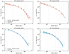 |
Fig. A.1. Pressure profiles in our work and literature works providing nonparametric determinations using SZ data (Ghirardini et al. 2019; Sayers et al. 2023). Errors on the estimates from other works are shown when available. Vertical dotted gray lines show the placement of the knots. Our profiles show a generally good agreement with results from other authors using independent data. |
Appendix B: Population analysis diagnostics plots
 |
Fig. B.1. Marginal posterior distribution (kernel density estimate) and trace plots of the population-level parameters. Each line refers to a different walker in the MCMC. |
The overdensity r500 is defined as the radius within which the average density is 500 times the critical density at the cluster’s redshift.
All Tables
Population-averaged pressure and intrinsic scatter values for the entire studied sample and for the morphological classes.
Sample of galaxy clusters and estimated parameters in the population analysis. The full table is available at CDS.
All Figures
|
Fig. 1. Studied sample (colored points) and entire SPT catalog (gray points, Bocquet et al. 2019). Gray points within the redshift-mass selection area did not meet the S/N or footprint constraints. Crosses indicate galaxy clusters that were subsequently removed from our sample. |
| In the text | |
|
Fig. 2. Derivation of r500 for two galaxy clusters, SPT-CLJ0051-4834 (left panel) and SPT-CLJ0328-5541 (right panel), shown as examples. Integrating the model ensures regularity in the case of noisy data (left panel) and does not affect high-quality data (right panel). |
| In the text | |
|
Fig. 3. Comparison of our estimates of r500 (y axis) with Planck for the 38 clusters in common (left panel) and with SPT for the entire sample (right panel). Our r500 values are strongly correlated with the Planck ones, while a larger scatter is observed when compared with SPT. No morphology-dependent trend is observed. |
| In the text | |
|
Fig. 4. Distribution of the reduced chi-square χν = 92 of the 58 individual fits and the population fit of 55 clusters. The red outlier with χν2 > 7 is SPT-CLJ0405-4916, which is characterized by a highly oscillating surface brightness distribution in its outermost region, while our background model, the pedestal, is a constant. For this reason, we excluded it from the population analysis. |
| In the text | |
|
Fig. 5. Distribution of the number of resolution elements, θ500/HWHM, across the initial sample of 58 objects. Because of our careful sample selection in mass and redshift, all clusters have θ500/HWHM > 5, i.e., are well resolved. The two clusters with θ500/HWHM > 30 are excluded from later analyses because of the high computational time required to include them in the hierarchical model. |
| In the text | |
|
Fig. 6. Resolution of galaxy clusters in our sample and in works that analyze galaxy clusters using only SZ instruments (Sayers et al. 2016; Pointecouteau et al. 2021; Melin & Pratt 2023). Compared to other studies, our selection focuses on well-resolved clusters. |
| In the text | |
|
Fig. 7. Integrated Compton parameter |
| In the text | |
|
Fig. 8. Surface brightness profiles of two clusters, taken from the population analysis. Vertical dotted gray lines show the placement of the knots, whereas the horizontal one indicates the estimated pedestal level. The plots highlight that our radial profile parametrization is adequate for these two clusters. Figure 4 quantifies the fit for the entire sample. |
| In the text | |
|
Fig. 9. Pressure profiles of the two clusters in Fig. 8. Vertical dotted gray lines show the placement of the knots. The plot highlights a marked change in concavity around the third interpolation knot. |
| In the text | |
|
Fig. 10. Joint and marginal posterior distributions for the population-averaged pressure parameters lgPk (top panel) and intrinsic scatters σint, k (bottom panel) at the five radii (interpolation knots). Dashed blue lines represent the median values. In the diagonal panels, vertical dotted blue lines indicate the 68% uncertainty interval, while dashed black lines represent the adopted prior. All parameters show little correlation, due to our choice of the radial profile modelization and the knots spacing. Prior distributions have a negligible impact on the posterior distributions. |
| In the text | |
|
Fig. 11. Correlation matrix for all 340 fit parameters. Most parameters show little covariance, except between the pressures of the two inner knots and between the pressures at the last knot and the pedestal parameters (see text for details). These low correlations contrast with those observed in the fit using a gNFW model (see Fig. 18). |
| In the text | |
|
Fig. 12. Pressure profiles (top panel) and intrinsic scatter (top and central panels) of our population analysis. The scatter is minimal at 0.4r500 ≤ r ≤ 0.7r500. The bottom panel shows the number of objects contributing at each radius. |
| In the text | |
|
Fig. 13. Individual pressure parameters lgPk, i (points with error bars) at the five knots (marked on the right y axis). Horizontal lines represent the population-averaged pressure estimates lgPk (solid lines) with their errors (shaded areas), and intrinsic scatter estimates (dotted lines). |
| In the text | |
|
Fig. 14. Individual pressure parameters lgPk, i (points with error bars) at the five knots (marked on the right y axis) as a function of the cluster’s P500. Horizontal lines represent the population-averaged pressure estimates lgPk (solid lines) with their errors (shaded areas), and intrinsic scatter estimates (dotted lines). |
| In the text | |
|
Fig. 15. Probability density function for the posterior and prior distributions of γP. A Bayes factor of 16.5 is moderately in favor of no dependence on P500. |
| In the text | |
|
Fig. 16. Pressure profiles (top panel) and intrinsic scatter (top and central panels) of regular and disturbed clusters. Error bars and shading as in Fig. 12. Points are slightly horizontally offset for clarity. Regular clusters seem to show a lower scatter at r ≥ 0.4r500 and a more peaked profile at the center. The bottom panel shows the number of objects contributing at each radius. |
| In the text | |
|
Fig. 17. Pressure profiles (top panel) and intrinsic scatters (bottom panel) for our sample and literature works, with literature errors omitted from the top panel for clarity. Within r500, our profile is ∼12% lower than the UPP, close to what is needed to remove the tension in cosmological parameters derived from CMB and Planck SZ cluster counts (Ruppin et al. 2019). The steep decline of our pressure profile beyond r500 is consistent with the deficit reported by Anbajagane et al. (2022), interpreted as a shock-induced thermal nonequilibrium between electrons and ions. Regarding the scatter, the three radial profiles are consistent up to 0.4r500. Beyond this radius, Sayers et al. (2023) report the highest scatter, while our analysis yields the lowest. |
| In the text | |
|
Fig. 18. Correlation matrix for all 340 fit parameters in an analysis performed assuming a gNFW model for the pressure profile. Many parameters show a strong level of covariance, much higher than with our pressure parametrization, whose correlation matrix is shown in Fig. 11. |
| In the text | |
|
Fig. A.1. Pressure profiles in our work and literature works providing nonparametric determinations using SZ data (Ghirardini et al. 2019; Sayers et al. 2023). Errors on the estimates from other works are shown when available. Vertical dotted gray lines show the placement of the knots. Our profiles show a generally good agreement with results from other authors using independent data. |
| In the text | |
|
Fig. B.1. Marginal posterior distribution (kernel density estimate) and trace plots of the population-level parameters. Each line refers to a different walker in the MCMC. |
| In the text | |
Current usage metrics show cumulative count of Article Views (full-text article views including HTML views, PDF and ePub downloads, according to the available data) and Abstracts Views on Vision4Press platform.
Data correspond to usage on the plateform after 2015. The current usage metrics is available 48-96 hours after online publication and is updated daily on week days.
Initial download of the metrics may take a while.