| Issue |
A&A
Volume 702, October 2025
|
|
|---|---|---|
| Article Number | A155 | |
| Number of page(s) | 31 | |
| Section | Cosmology (including clusters of galaxies) | |
| DOI | https://doi.org/10.1051/0004-6361/202555551 | |
| Published online | 21 October 2025 | |
Euclid: Photometric redshift calibration performance with the clustering-redshifts technique in the Flagship 2 simulation⋆
1
Institut de Física d’Altes Energies (IFAE), The Barcelona Institute of Science and Technology, Campus UAB, 08193 Bellaterra (Barcelona), Spain
2
Serra Húnter Fellow, Departament de Física, Universitat Autònoma de Barcelona, E-08193 Bellaterra, Spain
3
Aix-Marseille Université, CNRS, CNES, LAM, Marseille, France
4
Ruhr University Bochum, Faculty of Physics and Astronomy, Astronomical Institute (AIRUB), German Centre for Cosmological Lensing (GCCL), 44780 Bochum, Germany
5
Departament de Física, Universitat Autònoma de Barcelona, 08193 Bellaterra (Barcelona), Spain
6
Centro de Investigaciones Energéticas, Medioambientales y Tecnológicas (CIEMAT), Avenida Complutense 40, 28040 Madrid, Spain
7
Port d’Informació Científica, Campus UAB, C. Albareda s/n, 08193 Bellaterra (Barcelona), Spain
8
Max Planck Institute for Extraterrestrial Physics, Giessenbachstr. 1, 85748 Garching, Germany
9
Department of Astronomy, University of Geneva, ch. d’Ecogia 16, 1290 Versoix, Switzerland
10
Institute of Cosmology and Gravitation, University of Portsmouth, Portsmouth PO1 3FX, UK
11
Institució Catalana de Recerca i Estudis Avançats (ICREA), Passeig de Lluís Companys 23, 08010 Barcelona, Spain
12
ESAC/ESA, Camino Bajo del Castillo, s/n., Urb. Villafranca del Castillo, 28692 Villanueva de la Cañada, Madrid, Spain
13
School of Mathematics and Physics, University of Surrey, Guildford, Surrey GU2 7XH, UK
14
INAF-Osservatorio Astronomico di Brera, Via Brera 28, 20122 Milano, Italy
15
INAF-Osservatorio di Astrofisica e Scienza dello Spazio di Bologna, Via Piero Gobetti 93/3, 40129 Bologna, Italy
16
IFPU, Institute for Fundamental Physics of the Universe, Via Beirut 2, 34151 Trieste, Italy
17
INAF-Osservatorio Astronomico di Trieste, Via G. B. Tiepolo 11, 34143 Trieste, Italy
18
INFN, Sezione di Trieste, Via Valerio 2, 34127 Trieste TS, Italy
19
SISSA, International School for Advanced Studies, Via Bonomea 265, 34136 Trieste TS, Italy
20
Centre National d’Etudes Spatiales – Centre spatial de Toulouse, 18 avenue Edouard Belin, 31401 Toulouse Cedex 9, France
21
Dipartimento di Fisica e Astronomia, Università di Bologna, Via Gobetti 93/2, 40129 Bologna, Italy
22
INFN-Sezione di Bologna, Viale Berti Pichat 6/2, 40127 Bologna, Italy
23
INAF-Osservatorio Astronomico di Padova, Via dell’Osservatorio 5, 35122 Padova, Italy
24
Dipartimento di Fisica, Università di Genova, Via Dodecaneso 33, 16146 Genova, Italy
25
INFN-Sezione di Genova, Via Dodecaneso 33, 16146 Genova, Italy
26
Department of Physics "E. Pancini", University Federico II, Via Cinthia 6, 80126 Napoli, Italy
27
INAF-Osservatorio Astronomico di Capodimonte, Via Moiariello 16, 80131 Napoli, Italy
28
Dipartimento di Fisica, Università degli Studi di Torino, Via P. Giuria 1, 10125 Torino, Italy
29
INFN-Sezione di Torino, Via P. Giuria 1, 10125 Torino, Italy
30
INAF-Osservatorio Astrofisico di Torino, Via Osservatorio 20, 10025 Pino Torinese (TO), Italy
31
INAF-IASF Milano, Via Alfonso Corti 12, 20133 Milano, Italy
32
INAF-Osservatorio Astronomico di Roma, Via Frascati 33, 00078 Monteporzio Catone, Italy
33
INFN-Sezione di Roma, Piazzale Aldo Moro, 2 – c/o Dipartimento di Fisica, Edificio G. Marconi, 00185 Roma, Italy
34
Institute for Theoretical Particle Physics and Cosmology (TTK), RWTH Aachen University, 52056 Aachen, Germany
35
Institute of Space Sciences (ICE, CSIC), Campus UAB, Carrer de Can Magrans, s/n, 08193 Barcelona, Spain
36
Institut d’Estudis Espacials de Catalunya (IEEC), Edifici RDIT, Campus UPC, 08860 Castelldefels, Barcelona, Spain
37
INFN section of Naples, Via Cinthia 6, 80126 Napoli, Italy
38
Institute for Astronomy, University of Hawaii, 2680 Woodlawn Drive, Honolulu, HI 96822, USA
39
Dipartimento di Fisica e Astronomia “Augusto Righi” – Alma Mater Studiorum Università di Bologna, Viale Berti Pichat 6/2, 40127 Bologna, Italy
40
Instituto de Astrofísica de Canarias, Vía Láctea, 38205 La Laguna, Tenerife, Spain
41
Institute for Astronomy, University of Edinburgh, Royal Observatory, Blackford Hill, Edinburgh EH9 3HJ, UK
42
Jodrell Bank Centre for Astrophysics, Department of Physics and Astronomy, University of Manchester, Oxford Road, Manchester M13 9PL, UK
43
European Space Agency/ESRIN, Largo Galileo Galilei 1, 00044 Frascati, Roma, Italy
44
Université Claude Bernard Lyon 1, CNRS/IN2P3, IP2I Lyon, UMR 5822, Villeurbanne, F-69100, France
45
Institut de Ciències del Cosmos (ICCUB), Universitat de Barcelona (IEEC-UB), Martí i Franquès 1, 08028 Barcelona, Spain
46
UCB Lyon 1, CNRS/IN2P3, IUF, IP2I Lyon, 4 rue Enrico Fermi, 69622 Villeurbanne, France
47
Departamento de Física, Faculdade de Ciências, Universidade de Lisboa, Edifício C8, Campo Grande, PT1749-016 Lisboa, Portugal
48
Instituto de Astrofísica e Ciências do Espaço, Faculdade de Ciências, Universidade de Lisboa, Campo Grande, 1749-016 Lisboa, Portugal
49
Université Paris-Saclay, CNRS, Institut d’astrophysique spatiale, 91405 Orsay, France
50
Aix-Marseille Université, CNRS/IN2P3, CPPM, Marseille, France
51
INAF-Istituto di Astrofisica e Planetologia Spaziali, via del Fosso del Cavaliere, 100, 00100 Roma, Italy
52
Space Science Data Center, Italian Space Agency, via del Politecnico snc, 00133 Roma, Italy
53
INFN-Bologna, Via Irnerio 46, 40126 Bologna, Italy
54
School of Physics, HH Wills Physics Laboratory, University of Bristol, Tyndall Avenue, Bristol BS8 1TL, UK
55
Universitäts-Sternwarte München, Fakultät für Physik, Ludwig-Maximilians-Universität München, Scheinerstrasse 1, 81679 München, Germany
56
FRACTAL S.L.N.E., calle Tulipán 2, Portal 13 1A, 28231 Las Rozas de Madrid, Spain
57
Jet Propulsion Laboratory, California Institute of Technology, 4800 Oak Grove Drive, Pasadena, CA 91109, USA
58
Department of Physics, Lancaster University, Lancaster LA1 4YB, UK
59
Technical University of Denmark, Elektrovej 327, 2800 Kgs. Lyngby, Denmark
60
Cosmic Dawn Center (DAWN), Denmark
61
Max-Planck-Institut für Astronomie, Königstuhl 17, 69117 Heidelberg, Germany
62
NASA Goddard Space Flight Center, Greenbelt, MD 20771, USA
63
Department of Physics and Astronomy, University College London, Gower Street, London WC1E 6BT, UK
64
Department of Physics and Helsinki Institute of Physics, Gustaf Hällströmin katu 2, 00014 University of Helsinki, Finland
65
Université de Genève, Département de Physique Théorique and Centre for Astroparticle Physics, 24 quai Ernest-Ansermet, CH-1211 Genève 4, Switzerland
66
Department of Physics, P.O. Box 64 00014 University of Helsinki, Finland
67
Helsinki Institute of Physics, Gustaf Hällströmin katu 2, University of Helsinki, Helsinki, Finland
68
Laboratoire d’etude de l’Univers et des phenomenes eXtremes, Observatoire de Paris, Université PSL, Sorbonne Université, CNRS, 92190 Meudon, France
69
Institute of Theoretical Astrophysics, University of Oslo, P.O. Box 1029 Blindern 0315 Oslo, Norway
70
SKA Observatory, Jodrell Bank, Lower Withington, Macclesfield, Cheshire SK11 9FT, UK
71
Centre de Calcul de l’IN2P3/CNRS, 21 avenue Pierre de Coubertin, 69627 Villeurbanne Cedex, France
72
Dipartimento di Fisica “Aldo Pontremoli”, Università degli Studi di Milano, Via Celoria 16, 20133 Milano, Italy
73
INFN-Sezione di Milano, Via Celoria 16, 20133 Milano, Italy
74
University of Applied Sciences and Arts of Northwestern Switzerland, School of Computer Science, 5210 Windisch, Switzerland
75
Universität Bonn, Argelander-Institut für Astronomie, Auf dem Hügel 71, 53121 Bonn, Germany
76
Dipartimento di Fisica e Astronomia “Augusto Righi” – Alma Mater Studiorum Università di Bologna, via Piero Gobetti 93/2, 40129 Bologna, Italy
77
Department of Physics, Institute for Computational Cosmology, Durham University, South Road, Durham DH1 3LE, UK
78
Infrared Processing and Analysis Center, California Institute of Technology, Pasadena, CA 91125, USA
79
Université Paris Cité, CNRS, Astroparticule et Cosmologie, 75013 Paris, France
80
CNRS-UCB International Research Laboratory, Centre Pierre Binétruy, IRL2007, CPB-IN2P3, Berkeley, USA
81
University of Applied Sciences and Arts of Northwestern Switzerland, School of Engineering, 5210 Windisch, Switzerland
82
Institut d’Astrophysique de Paris, 98bis Boulevard Arago, 75014 Paris, France
83
Institut d’Astrophysique de Paris, UMR 7095, CNRS, and Sorbonne Université, 98 bis boulevard Arago, 75014 Paris, France
84
Institute of Physics, Laboratory of Astrophysics, Ecole Polytechnique Fédérale de Lausanne (EPFL), Observatoire de Sauverny, 1290 Versoix, Switzerland
85
Telespazio UK S.L. for European Space Agency (ESA), Camino bajo del Castillo, s/n, Urbanizacion Villafranca del Castillo, Villanueva de la Cañada, 28692 Madrid, Spain
86
European Space Agency/ESTEC, Keplerlaan 1, 2201 AZ Noordwijk, The Netherlands
87
DARK, Niels Bohr Institute, University of Copenhagen, Jagtvej 155, 2200 Copenhagen, Denmark
88
Université Paris-Saclay, Université Paris Cité, CEA, CNRS, AIM, 91191 Gif-sur-Yvette, France
89
Institute of Space Science, Str. Atomistilor, nr. 409 Măgurele, Ilfov 077125, Romania
90
Consejo Superior de Investigaciones Cientificas, Calle Serrano 117, 28006 Madrid, Spain
91
Universidad de La Laguna, Departamento de Astrofísica, 38206 La Laguna, Tenerife, Spain
92
Dipartimento di Fisica e Astronomia “G. Galilei”, Università di Padova, Via Marzolo 8, 35131 Padova, Italy
93
INFN-Padova, Via Marzolo 8, 35131 Padova, Italy
94
Institut für Theoretische Physik, University of Heidelberg, Philosophenweg 16, 69120 Heidelberg, Germany
95
Institut de Recherche en Astrophysique et Planétologie (IRAP), Université de Toulouse, CNRS, UPS, CNES, 14 Av. Edouard Belin, 31400 Toulouse, France
96
Université St Joseph; Faculty of Sciences, Beirut, Lebanon
97
Departamento de Física, FCFM, Universidad de Chile, Blanco Encalada 2008, Santiago, Chile
98
Universität Innsbruck, Institut für Astro- und Teilchenphysik, Technikerstr. 25/8, 6020 Innsbruck, Austria
99
Satlantis, University Science Park, Sede Bld 48940, Leioa-Bilbao, Spain
100
Department of Physics, Royal Holloway, University of London, TW20 0EX, UK
101
Instituto de Astrofísica e Ciências do Espaço, Faculdade de Ciências, Universidade de Lisboa, Tapada da Ajuda, 1349-018 Lisboa, Portugal
102
Cosmic Dawn Center (DAWN)
103
Niels Bohr Institute, University of Copenhagen, Jagtvej 128, 2200 Copenhagen, Denmark
104
Universidad Politécnica de Cartagena, Departamento de Electrónica y Tecnología de Computadoras, Plaza del Hospital 1, 30202 Cartagena, Spain
105
Centre for Information Technology, University of Groningen, PO Box 11044 9700 CA Groningen, The Netherlands
106
Kapteyn Astronomical Institute, University of Groningen, PO Box 800 9700 AV Groningen, The Netherlands
107
INAF, Istituto di Radioastronomia, Via Piero Gobetti 101, 40129 Bologna, Italy
108
Department of Physics, Oxford University, Keble Road, Oxford OX1 3RH, UK
109
Aurora Technology for European Space Agency (ESA), Camino bajo del Castillo, s/n, Urbanizacion Villafranca del Castillo, Villanueva de la Cañada, 28692 Madrid, Spain
110
INAF-Osservatorio Astronomico di Brera, Via Brera 28, 20122 Milano, Italy, and INFN-Sezione di Genova, Via Dodecaneso 33, 16146 Genova, Italy
111
ICL, Junia, Université Catholique de Lille, LITL, 59000 Lille, France
112
ICSC – Centro Nazionale di Ricerca in High Performance Computing, Big Data e Quantum Computing, Via Magnanelli 2, Bologna, Italy
⋆⋆ Corresponding author: This email address is being protected from spambots. You need JavaScript enabled to view it.
Received:
16
May
2025
Accepted:
28
July
2025
Abstract
Aims. The precision of cosmological constraints from imaging surveys hinges on an accurately estimated redshift distribution n(z) of the tomographic bins, especially their mean redshifts. We assess the effectiveness of the clustering-redshifts technique in constraining Euclid tomographic redshift bins to meet the target uncertainty of σ(⟨z⟩) < 0.002(1 + z). We inferred these mean redshifts from the small-scale angular clustering of Euclid galaxies, which were distributed into bins with spectroscopic samples localised in narrow redshift slices.
Methods. We generated spectroscopic mocks from the Flagship2 simulation for the Baryon Oscillation Spectroscopic Survey (BOSS), the Dark Energy Spectroscopic Instrument (DESI), and the Euclid Near-Infrared Spectrometer and Photometer (NISP) spectroscopic survey. We evaluated and optimised the clustering-redshifts pipeline, and we introduced a new method for measuring the photometric galaxy bias (clustering), which is the primary limitation of this technique.
Results. We have successfully constrained the means and standard deviations of the redshift distributions for all of the tomographic bins (with a maximum photometric redshift of 1.6). We achieved precision beyond the required thresholds. We have identified the main sources of bias, particularly the impact of the one-halo galaxy distribution, which imposed the minimal separation scale to be larger than 1.5 Mpc for evaluating cross-correlations. These results demonstrate that clustering-redshifts can meet the precision requirements for Euclid, and we highlighted several avenues for future improvements.
Key words: methods: data analysis / methods: statistical / techniques: photometric / techniques: spectroscopic / large-scale structure of Universe
This paper is published on behalf of the Euclid Consortium.
© The Authors 2025
 Open Access article, published by EDP Sciences, under the terms of the Creative Commons Attribution License (https://creativecommons.org/licenses/by/4.0), which permits unrestricted use, distribution, and reproduction in any medium, provided the original work is properly cited.
This article is published in open access under the Subscribe to Open model. This email address is being protected from spambots. You need JavaScript enabled to view it. to support open access publication.
1. Introduction
The Euclid space telescope is currently mapping the positions and shapes of billions of galaxies. This provides data that are critical to understand the large-scale structure of the Universe, in particular, the mysterious nature of dark matter and dark energy (Euclid Collaboration: Mellier et al. 2025). Through its imaging survey, Euclid measures the flux of galaxies in the visible and near-infrared wavelengths using broadband filters. Additionally, it determines spectroscopic redshifts for a subset of galaxies via slitless spectroscopy, targeting emission-line galaxies (ELGs). These data will enable the precise determination of cosmological parameters and models, primarily through the study of galaxy clustering, galaxy-galaxy lensing, and cosmic shear (Euclid Collaboration: Blanchard et al. 2020), with galaxy samples divided into approximate line-of-sight tomographic bins.
It is essential to accurately estimate the redshift distributions of these galaxy samples to interpret cosmological measurements correctly (see e.g. Huterer et al. 2006; Bordoloi et al. 2010; Hildebrandt et al. 2021; Stölzner et al. 2021). The vast amount of forthcoming data means that it is not feasible to obtain spectroscopic redshifts for every individual galaxy because spectroscopy of large samples is time-consuming and costly. Photometric surveys provide redshift estimates for each galaxy based on multi-band photometry of that galaxy, a technique called photometric redshift, or photo-z. A large variety of photo-z methods exists (e.g. Tanaka et al. 2018; Salvato et al. 2019; Euclid Collaboration: Ilbert et al. 2021; Euclid Collaboration: Desprez et al. 2020). The photometric information can also be used to produce redshift estimates using scheme based on a self-organising map (hereafter, SOM), which allows a more general control over all the known potential sources of uncertainties that affect the estimates (Wright et al. 2020a,b; Myles et al. 2021; Giannini et al. 2024; Campos et al. 2024; Wright et al. 2025; Roster et al. 2025). The degeneracies between colours and redshift, however, and unrepresentative spectroscopic samples for training and calibration ultimately limit the performance of photometric methods (Wright et al. 2020a; Hartley et al. 2020).
Clustering-based redshift estimation methods offer another alternative to infer redshift distributions (see e.g. Newman 2008; Ménard et al. 2013; McQuinn & White 2013; Morrison et al. 2017; Scottez et al. 2018; Gatti et al. 2018; van den Busch et al. 2020; Hildebrandt et al. 2021; Gatti et al. 2022; Cawthon et al. 2022; Rau et al. 2023; Wright et al. 2025). Unlike photo-z, clustering-redshifts techniques statistically infer the redshift properties for entire bins instead of individual galaxies. Furthermore, this approach is independent of photometric uncertainties, observations over smaller deep fields, or representative spectroscopic samples.
The clustering-redshifts method relies on angular cross-correlations between spectroscopic samples, with secure redshifts, and photometric samples. Samples that overlap in redshift trace the same underlying dark matter field and are consequently correlated in their position. The amplitude of this angular correlation provides insight into their redshift overlap, which results in the measurement of the redshift distribution of the photometric samples. This amplitude is degenerate with galaxy biases (of both samples), however, which makes the measurement of these biases, and their redshift evolution, a critical step (McQuinn & White 2013; Gatti et al. 2018; Naidoo et al. 2023). While the galaxy bias for the spectroscopic sample can be directly constrained through auto-correlation functions, it is more challenging to estimate the galaxy bias for the photometric sample (van den Busch et al. 2020; Cawthon et al. 2022), and is sometimes evaluated using simulations (Gatti et al. 2022).
The precision of the clustering-redshifts method depends on the redshift and sky overlap of the photometric and spectroscopic data, but also on range of the clustering angular scale. To achieve the primary science goal of Euclid, the uncertainty on the mean redshift, σ(⟨z⟩), for each tomographic bin must remain below 0.002(1 + z) at 68% confidence (Laureijs et al. 2011). Naidoo et al. (2023) found that clustering-redshifts would be able to reach the statistical uncertainties required by Euclid for a sufficiently large sky overlap, typically several hundreds of deg2, when analysing scales from 100 kpc to 1 Mpc, although systematic biases limit the accuracy. In particular, there were some unknown residual biases for high-redshift bins with their methods or simulated data.
This paper aims to re-evaluate the potential of photometric-spectroscopic cross-correlations as a core component of the redshift calibration for Euclid. Our method may be seen as a continuation, and a substantial improvement from Naidoo et al. (2023). We used 5000 deg2 of simulated data from the Euclid Flagship2 simulation (Euclid Collaboration: Castander et al. 2025). Our goal is to evaluate the uncertainties associated with the clustering-redshifts calibration through a realistic framework, and to determine the limitation of the method. We created spectroscopic mock samples for the Dark Energy Spectroscopic Instruments (DESI), or alternatively, for the 4-metre Multi-Object Spectroscopic Telescope (4MOST), the Baryon Oscillation Spectroscopic Survey (BOSS), and Euclid. We assessed the potential systematic effects on the measurement, introduced a new method to measure photometric galaxy bias, optimised the clustering-z pipeline, and derived methods for inferring the redshift constraints from the amplitude of two-point correlations. We assumed the same flat ΛCDM cosmology as was used for the simulation, with Ωm = 0.319, Ωb = 0.049, ΩΛ = 0.681, As = 2.1 × 10⁻⁹, ns = 0.96, σ8 = 0.813, and h = 0.67. Our code is publicly available1.
This paper is organised as follows. In Sect. 2 we describe the Flagship2 simulation and the mocks we generated to mimic Euclid and spectroscopic data. In Sect. 3 we give a detailed overview of angular clustering, its application to clustering redshifts, and potential sources of errors. In Sect. 4 we present the different tests we ran to optimise the pipeline and address potential sources of bias. Finally in Sect. 5 we apply the results pipeline to realistic Euclid tomographic bins and compare our results with previous work and the requirements.
2. Simulated data
To assess the performance of the Euclid clustering-redshifts method, we constructed simulated datasets that were as similar as possible to the observational datasets. In this section, we describe how these samples can be generated from the Flagship simulation.
2.1. The Flagship simulation and survey mocks
For this study, we used the second edition of the Flagship catalogue (version 2.1.10), which was presented in detail in Euclid Collaboration: Castander et al. (2025). The Euclid Flagship N-body dark matter simulation comprises a simulation box measuring 3600 h−1 Mpc on each side, containing 4 trillion particles. This simulation is the largest N-body simulation performed to date and encompasses a cosmological volume comparable to what the telescope will survey. It enables precise resolution of 16 billion dark matter haloes, which host even the faintest galaxies that Euclid intends to observe. They are identified with the ROCKSTAR halo finder (Behroozi et al. 2013). From this dark matter simulation, a synthetic galaxy catalogue was generated with a prescription including the halo occupation distribution (HOD) and abundance matching (AM) techniques, as well as empirical relations between galaxy properties (Euclid Collaboration: Castander et al. 2025).
Each galaxy entry in the catalogue is associated with observed fluxes for multiple survey bands, observed spectroscopic redshift (zspec, including peculiar velocity), photometric redshift estimates (zp), true redshift (ztrue), true and magnified coordinates, lensing convergence κ and shear γ = γ1 + iγ2. Source photometry is provided in terms of fluxes F (in erg s−1 cm−2 Hz−1) rather than in magnitude m. We generate magnified fluxes as in Lepori et al. (2025), using the relation
 (1)
(1)
We do not include the Doppler effect, which is usually a very small correction, and note that the effect of magnification is achromatic: that is, it is the same for for the different bands and it cancels for colours.
We need mock samples Euclid-like photometric galaxies, Euclid-like Near-Infrared Spectrometer and Photometer Survey (NISP-S) galaxies, and other spectroscopic tracers (Dawson et al. 2013; Adame et al. 2024): BOSS-like low-redshift (LOWZ) and constant mass (CMASS) galaxies; DESI-like bright galaxies (BGs), luminous red galaxies (LRGs), and ELGs. The selection of each sample is described in the following sections. Differences in the redshift distributions or colours of observational and simulated galaxy samples may stem from the incompleteness of the target sample or limitations in the simulation’s ability to replicate accurate colour distributions. As in Naidoo et al. (2023), systematic issues such as variable photometry, variable survey depth, and complex masks are not addressed. We generated one version of these samples with unmagnified fluxes, which will be our default samples, and one version with the same cuts on magnified photometry. We produced numerous fast generations of galaxy catalogues, varying sample definitions and areas, using the web application CosmoHub (Carretero et al. 2017; Tallada et al. 2020). Our photometric and spectroscopic samples are plotted in Fig. 1.
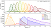 |
Fig. 1. Top: Simulated true-redshift distribution of each of the first ten tomographic bins (zphoto < 1.6). Bottom: Simulated redshift distribution of the spectroscopic samples from the BOSS, DESI, and Euclid surveys. The lack of spectroscopic samples for zspec > 1.8 imposes the zphoto < 1.6 condition for clustering-redshifts calibration. |
2.2. Euclid photometric sample
The photometric sample was constructed by imposing an upper limit on the IE magnitude (Euclid Collaboration: Cropper et al. 2025), set at 24.5, to emulate the expected performance of Euclid (Laureijs et al. 2011). Several algorithms exist for evaluating the photometric redshift. We used the Deep-z estimate which was run for the full catalogue. The Deep-z photo-z method, introduced for the Physics of the Accelerating Universe (PAU) survey in Eriksen et al. (2020), uses a linear neural network with a mixture density network for predicting the redshift distributions. The network has not been pretrained on simulations, avoiding potential problems with over-fitting by using too similar simulations. The network was trained with 20 000 simulated galaxies, magnitude-limited to iLSST < 23 without colour selection. The training used the Legacy Survey of Space and Time (LSST; LSST Science Collaboration 2009) bands plus Euclid near-infrared (NIR) bands, a batch size of 200 and 1000 epochs with varying learning rates. The photometric noise added to noiseless fluxes corresponds to the depth forecast in the southern hemisphere for the Euclid DR3 time. The limiting magnitudes at 10σ are 24.4, 25.6, 25.7, 25.0, 24.3, 24.3 for the ugrizy bands of LSST, and 25.0, 23.5, 23.5, 23.5 for the IE, YE, JE, HE bands of Euclid (Euclid Collaboration: Cropper et al. 2025; Euclid Collaboration: Jahnke et al. 2025).
LSST photometry will not be available over the whole Euclid footprint, and therefore the photometry will be different in the northern region where photometry will be provided by UNIONS (Gwyn et al. 2025). However, for clustering redshifts, we do not depend on photo-z quality except for the tomographic bin definitions and photometric bias correction. Spectroscopy from DESI and BOSS-eBOSS will be available in the north, and 4MOST will provide DESI-like samples in the south. Thus, photometric angular anisotropies will be tested in practice.
We selected galaxies with photo-z between 0.2 and 1.6. We did not consider galaxies with a photo-z higher than 1.6 because we do not have large spectroscopic samples at redshifts greater than 1.8. Future studies could test the possibility of using quasar galaxy samples from BOSS, eBOSS, DESI, and 4MOST (Palanque-Delabrouille et al. 2016; Yèche et al. 2020) for high-z calibration. BOSS and eBOSS quasars were used for the clustering-redshifts DES calibration, but as a complement to ELGs and LRGs data sets for z < 1.1 (Gatti et al. 2022; Giannini et al. 2024). The low density of this sample, and clustering properties at high-z, require a dedicated study. Nonetheless, eBOSS QSOs will be used for the high-z calibration of the final DES data for 0.8 < z < 2.2 (d’Assignies et al., in prep.); thus one expects that DESI QSOs could be used up to z = 3.5 for Euclid. Generating DESI QSO mocks and testing clustering-redshifts with them is left for future work.
We produced ten tomographic bins with approximately equal numbers of galaxies, through photo-z cuts. The fiducial Euclid survey at data release 3 plans to use 13 bins instead of ten, and we can assume that three of these bins will contain galaxies with zp > 1.6. The true redshift distributions (that we want to measure) of our simulated tomographic bins are reported in Fig. 1.
2.3. Euclid NISP sample
We defined mock NISP-S samples in Flagship2 by selecting galaxies with H α fluxes greater than 2 × 10⁻¹⁶erg cm−2 s−1 (Laureijs et al. 2011), in the expected redshift range, with
 (2)
(2)
 (3)
(3)
We obtained a galaxy density of 1990 deg−2. Unlike the other spectroscopic samples, this dataset is expected to suffer from a significant level of contamination by interlopers (Euclid Collaboration: Le Brun et al. 2025, Risso et al., in prep.). These interlopers are galaxies whose true redshifts differ substantially from their estimated values, leading to incorrect associations in redshift space. Although our analysis did not employ realistic mocks that include such contaminants, we adopted the approach of Contarini et al. (2022): we uniformly down-sampled the galaxy catalogue, retaining only 60% of the originally selected galaxies. This down-sampled catalogue is then assumed to have 100% purity, effectively removing the impact of interlopers in our modelling. Thus, our fiducial density is 1200 deg−2 as the sample from Naidoo et al. (2023), which was generated with a brighter cut on the H α flux. This is a pessimistic sample from the precision point of view (i.e. fewer spectra means larger uncertainty on the redshift distribution reconstruction; cf. McQuinn & White 2013), but optimistic in terms of accuracy, because our sample is interloper free (Addison et al. 2019). Interlopers may significantly degrade the performance of clustering-redshifts if not taken into consideration, as they are not necessarily distributed randomly in redshift. Indeed, clustering-redshifts might be helpful to quantify the interlopers’ properties such as their fraction and redshift distribution, by cross-correlating them with spectroscopic samples which do not suffer from the same misidentification. We will explore these two aspects in future work.
2.4. BOSS LOWZ and CMASS samples
We replicated the BOSS colour-magnitude selections specified in Dawson et al. (2013) in Flagship, as in Naidoo et al. (2023). We first define
 (4)
(4)
 (5)
(5)
 (6)
(6)
There are two spectroscopic BOSS LRG samples: LOWZ and CMASS. They correspond to adjacent redshift intervals 0.15 ≤ zspec ≤ 0.43 and 0.43 < zspec ≤ 0.7, respectively, with true densities of about 30 deg−2 and 120 deg−2, respectively.
The LOWZ sample is defined by
 (7)
(7)
 (8)
(8)
 (9)
(9)
and the CMASS sample by
 (10)
(10)
 (11)
(11)
 (12)
(12)
We got LOWZ- and CMASS- like objects, with densities of 48.5 deg−2 and 164.3 deg−2. We then applied sparse sampling to get the desired densities. We refer to the joint LOWZ+CMASS sample as the BOSS sample in our study.
2.5. DESI samples
We generated DESI BG, LRG, and ELG mocks that mimic the sample characteristics reported in Adame et al. (2024). We associated these galaxy samples to the DESI survey, but similar samples are expected to be observed by 4MOST (Verdier et al. 2025). For BGs, and ELGs, we used the same cuts as Naidoo et al. (2023), which were based on DESI Collaboration (2016). For LRGs, we used a different selection to generate a sample covering the entire z < 1.1 redshift range. As we previously mentioned in Sect. 2.1, there is a mismatch in the Flagship2 colour distribution and data expectation, and using the same colour cuts can lead to some significant differences. We find this issue to be particularly problematic for LRGs. Therefore we did not apply the same selection as Adame et al. (2024), but rather we tried to closely reproduce the redshift distribution and galaxy properties with similar but modified cuts.
We selected the BG-like galaxies with
 (13)
(13)
 (14)
(14)
We adopted for LRGs the tailored cuts
 (15)
(15)
 (16)
(16)
 (17)
(17)
Finally, we selected ELGs with
 (18)
(18)
 (19)
(19)
 (20)
(20)
 (21)
(21)
 (22)
(22)
 (23)
(23)
These cuts provided BG-, LRG-, and ELG-like objects with densities of 850, 909, and 4158 deg−2. We achieved the fiducial densities 700, 550, and 1140 deg−2 with sparse sampling.
3. Theory and method
In this section, we provide a detailed description of the clustering-redshifts method. Our approach begins with an overview of galaxy clustering in Sect. 3.1. In Sect. 3.2 we explain how the clustering equations are simplified for some particular redshift distributions. We then apply this formalism to the clustering-redshifts context in Sect. 3.3. In Sect. 3.4, we explain how clustering-redshifts are evaluated with data in practice. Finally, in Sect. 3.5 we explain our strategy to deduce from the data-vectors constraints on the redshift distribution moments. In particular, in Sect. 3.5.1, we state the Euclid requirements for the np measurements, which must be fulfilled in order to provide robust constraints on cosmological parameters.
3.1. Angular galaxy clustering
In this section we provide a general introduction to photometric angular clustering, as a basis for the development of our clustering-redshifts method. It draws inspiration from many previous weak-lensing and clustering-z works such as Davis et al. (2018), Krause et al. (2021), Gatti et al. (2018, 2022), Cawthon et al. (2022), and Pandey et al. (2025).
3.1.1. Galaxy density contrast
The observed angular galaxy count of a sample a (photometric or spectroscopic) is
 (24)
(24)
where  is the mean (observed) galaxy count, and
  is the observed projected galaxy density contrast. It can be expressed as (Krause et al. 2021)
 (25)
(25)
where μ refers to magnification, RSD to redshift space distortion (in the linear regime2), and  to the line of sight projection of the three-dimensional (3D) galaxy density contrast δa(z, ⃗θ):
 (26)
(26)
where na(z) is the redshift distribution of the observed sample, normalised to unity, and function of the observed redshift. All these quantities are associated with observations, and they depend on survey properties (depth, masks etc.), but for clarity, we drop the “obs” index for the rest of our work, as we do not consider observational systematics. We also do not model relativistic corrections.
3.1.2. Angular two-point correlation function
The angular two-point correlation function of samples a and b (with possibly a = b) from the observed projected density contrast can be written as
 (27)
(27)
where ⟨…⟩ indicates an average over angular scales, and θ is now a scalar3. The dominant corrections (RSD×D; μ ×D) are already small with respect to the dominant term (D×D), and we decided to omit even smaller corrections (Krause et al. 2021; Gatti et al. 2022).
We will mainly focus on the D × D correlation. Since it corresponds to the leading order, we omit its D index in the rest of the article. The clustering two-point correlation can be expressed as
 (28)
(28)
 (29)
(29)
 (30)
(30)
where we have defined the 3D cross-correlation function ξab(za, zb, θ), and used ⟨δx⟩ = 0. While we have introduced the correlations as a function of sky separation θ, we can also express them as functions of the perpendicular comoving separation rp, defined as
 (31)
(31)
in the flat sky approximation, and small angle limit, where χ is the comoving radial distance (equal to the comoving angular-diameter distance with no spatial curvature). Working with rp instead of θ is relevant when making particular scale choices for evaluating the correlation, but the Python package we use, TreeCorr (Jarvis 2015) has angular separation as the default convention.
3.1.3. Moving to matter statistics with galaxy bias
For large-scale correlations, the linear galaxy bias provides a relation between the galaxy overdensity and the matter density field δm
 (32)
(32)
where bg is the galaxy sample bias, and δm is the matter density field. Under this approximation, the angular correlation function becomes,
 (33)
(33)
where ξm is the 3D matter two-point correlation.
Following the literature, we used the linear bias expression of Eq. (32) by default. It is worth noting, however, that the linear bias expression is expected to break at scales around 6 h−1 Mpc. In addition, the next-order expression would extend this scale range to around 4 h−1 Mpc (Pandey et al. 2020). Thus, none of the equations (linear or non-linear e.g. Appendix A) are properly adapted to the standard clustering-redshifts scale ranges, (0.1–1) h−1 Mpc, (0.5–1.5) h−1 Mpc or (1–5) h−1 Mpc. However, linear bias has been tested to give accurate enough modelling for clustering-redshifts analysis (Gatti et al. 2018, 2022; van den Busch et al. 2020; Cawthon et al. 2022; Naidoo et al. 2023). As a consequence, it is crucial to quantify and address potential deviations introduced in the reconstructed n(z). We will pay particular attention to the galaxy bias issue, nonlinear contributions, and the scale range choice.
3.1.4. Magnification
In this section, we describe the two magnification terms in Eq. (27),
 (34)
(34)
Magnification is a lensing effect due to the gravitational bending of distant source light by the matter between those sources and the observer (Krause et al. 2021; Elvin-Poole et al. 2023). It introduces an angular position correlation for galaxies distant in redshift because of the lensing of a high-z galaxy sample by the matter traced by a lower-z sample4. Fortunately, this effect, which breaks the naive hypothesis that in clustering-redshifts only galaxies close in redshift are correlated, can be modelled.
Magnification impacts the apparent position of galaxies and their density. In regions of positive convergence5, the apparent separation between any two points on a source plane is enlarged, leading the telescope to capture a larger apparent solid angle, consequently reducing the apparent galaxy density locally. Another effect of positive convergence is an increase in distant source flux received by the telescope, potentially resulting in a change in the number of galaxies passing through the selection function.
Magnification was taken into account for clustering-z in DES, through direct modelling of its effect, and simulation-based estimation of magnification coefficients (Gatti et al. 2022; Cawthon et al. 2022). Complete inclusion of magnification should include position magnification, flux magnification, and its impact on photo-z, which can be significant (Legnani et al., in prep.), but we restricted this work to position and flux magnification. We detail how magnification can be modelled in the Appendix B. Since the tomographic bins are expected to be narrower for Euclid than for DES, the effect of magnification is expected to be smaller, as illustrated by the toy examples in Appendix B. Therefore, we do not include magnification in our default modelling. We will reassess the need to incorporate magnification in future work, based on the properties of the data bins.
3.1.5. RSD
In the linear regime, RSD contributes to the projected galaxy density contrast through the apparent large-scale flow of galaxies across the redshift boundaries of the bins (Krause et al. 2021). Equivalently, the redshift distribution of galaxies as a function of the observed redshift is slightly different from the distribution as a function of the Hubble redshift. The latter should be used, however, as the modelling assumes isotropy through the correlation function ξ. Since the photometric tomographic bins are quite large, it would mainly affect the spectroscopic sample which is divided into narrow redshift slices; the narrower the slices, the larger the effect is. Therefore, only the term  may contribute to the two-point correlation of Eq. (27). We tested in Sect. 4.7 the bias induced by the use of the spec-z instead of true-z for the spectroscopic slicing, in the Flagship simulation, since peculiar velocities are included, cf. Sect. 2.1.
3.2. Impact of the galaxy redshift distribution and its modelling
A tomographic bin will be referred to as a sample p, without referring to the tomographic ID, as the latter is always explicit. Different spectroscopic samples are considered in this article from different simulated surveys and tracers, such as DESI ELGs. For a given survey tracer, we will additionally distribute the sample into redshift slices, with spectroscopic redshift cuts. For a given redshift slice, the galaxies will be referred to as sj, or {s, zj} with zj the mean of the redshift slice. We explore two cases for the modelling of the distribution and two-point correlations with a sliced spectroscopic sample.
3.2.1. Ideal case of a Dirac galaxy distribution
The situation often presented in clustering-redshifts literature (e.g. Gatti et al. 2022; Giannini et al. 2024) is the one of a sample localised in such a small redshift slice that it can be approximated by a Dirac distribution
 (35)
(35)
The cross-correlation with a second sample is then simplified to
 (36)
(36)
 (37)
(37)
with
 (38)
(38)
To go from Eq. (36) to Eq. (37), we assume the redshift evolution of the bias and distribution of the second sample is small in the support of ξm (i.e. in a small redshift interval centred in zi).
3.2.2. Realistic case: Spectroscopic sample into small redshift slices
Using the Limber approximation, Eq. (33) reduces to,
 (39)
(39)
where ξm is the same as in Eq. (38). In the standard scenario of clustering redshifts, the spectroscopic galaxy sample is localised within small redshift slices zi ± Δzi/2, so that the distribution can be approximated as uniform
 (40)
(40)
where Δzi is typically between 0.01 and 0.05. This modelling is of course only approximated true in practice, and would lead to some deviations which we will evaluate. In particular, under the assumption of constant galaxy bias across the redshift bin, the spectroscopic auto-correlation (b = a) becomes
 (41)
(41)
Thus, given a cosmology, waa provides a straightforward measurement of the spectroscopic galaxy bias. We note that this equation diverges as Δz → 0, and that, more generally, both our modelling and the Limber approximation are expected to become less accurate for narrower redshift bins and on larger angular scales (Simon 2007).
For b ≠ a, when the redshift evolution of the biases ba and bb and the redshift distribution nb is neglected, we obtain
 (42)
(42)
The superscript Limber-1-bin refers to the integration of the matter distribution over a redshift bin equal to the spectroscopic slice; we uses the Limber approximation too. If one further neglects the matter correlation variation over Δzi, one recovers the Dirac approximation Eq. (37); this is the approach of van den Busch et al. (2020), for example.
A limitation of Eq. (42) is the assumption that the redshift distribution nb is constant across the bin. In practice, nb could be larger near the bin edges and smaller near the centre (or the opposite), leading to an underestimation (resp. overestimation) of correlations with galaxies localised near zi ± Δzi. To address these issues without resorting to Eq. (39), we propose a correction by explicitly incorporating contributions from galaxies outside the spectroscopic redshift slice (three-bins):
 (43)
(43)
We introduce the phased correlations
 (44)
(44)
which account for the correlation of two bins of widths Δzi, separated by δz. Here, the three-bins modelling does not uses the Limber approximation. One can write Eq. (43) as
 (45)
(45)
with η0 = 1 and
 (46)
(46)
where ξm 0, ±Δzi is defined in Eq. (44). This formulation allows for a linear inference of ⃗n from the two-point correlation, which can be implemented in practice, unlike the Limber-full-z case where np(z) is integrated over, complicating the process.
3.2.3. Comparison of the correlation modelling
In the previous sections, we introduced four different approximations of the two-point correlation function described by Eq. (33):  ,
,  ,
,  , and
, and  . In this section, we investigate the differences between them with a toy model. We consider 10 samples ai, each with a step-n(z) distribution as given by Eq. (40), centred at zi = 0.325 + 0.05 i, with i = 0, 1…, 9, and Δzi = 0.05. For the redshift distribution of sample b we take a Gaussian (μ, σ) = (0.5, 0.08). This reproduces an idealistic case scenario of clustering-z calibration, with sample b representing the photometric data, and samples ai representing the spectroscopic data. Several of these n(z)s are plotted in the upper panel of Fig. 2. We assume a constant galaxy bias ba(z) = bb(z) = 1 for all samples, and evaluate correlation functions for rp = 2 Mpc (a scale standard for clustering-z analysis). We numerically evaluated the functions with the CCL library6 (Chisari et al. 2019). We used the default configuration, which is based on predictions from CLASS (Blas et al. 2011) and halofit (Takahashi et al. 2012) for the nonlinear power spectrum. We evaluated the functions at scales where we know the predictions are not completely precise because of the galaxy-halo connection, but as will be explicit in Sect. 3.3, this is expected to have little impact on real data.
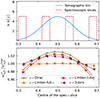 |
Fig. 2. Top: Redshift distribution of sample b in blue, and four out of the ten samples ai in red. Bottom: Deviation of approximated waib with respect to the exact one for the ten cross-correlations. |
In the lower panel of Fig. 2, we show the deviation of the four approximations to the “exact” correlation Eq. (33), for the samples ai, b. The level of the deviations depends on the nb(z) where the correlation is evaluated: we observe a larger deviation near the peak and for the tails. We evaluated the root mean square (RMS) of the deviation to 1 and got 0.022 (Dirac), 0.021 (Limber-1-bin), 0.013 (3-bins), and 0.002 (Limber-full-z). We can see that the Dirac and one-bin approximations are very close. Taking into consideration the correlations from bin neighbours with three-bins, we get an improvement of 40%. Finally, the best approximation is the Limber-full-z case [i.e. integrating n2(z) instead of assuming some effective values], with a deviation of 0.2% for individual points, and an RMS smaller by an order of magnitude to the Dirac and one-bin approximations.
In clustering-z studies, however, the redshift distribution np(z) is an unknown quantity that we aim to constrain from the measurement of wab. As a result, the Limber-full-z case is challenging to apply in practice, as the unknown np(z) is integrated over. In contrast, for the Dirac and one-bin cases, np(zi) enters the calculation linearly, making it easier to extract information. The same applies to the three-bins approximation, which provides a better approximation, as we have demonstrated.
3.3. Application to clustering redshifts
In the context of clustering redshifts, a photometric sample has an unknown redshift distribution np(z). To reconstruct it, we measure the cross-correlations with spectroscopic samples, distributed into fine redshift slices (usually 0.02 ≤ Δz ≤ 0.05). The distribution of these spectroscopic samples is assumed to be constant in each of these smaller slices (see Eq. 40). The amplitude of the photometric distribution at redshift zi can then be inferred linearly from the cross-correlation function between a spectroscopic bin centred in zi and the photometric sample [noted wsp(zi, θ) instead of wsip(θ)], assuming the Dirac modelling Eq. (37):
 (47)
(47)
One can write a similar expression for the one-bin and three-bins modelling, as described in Sect. 3.2.3.
The spectroscopic bias can be measured with the spectroscopic auto-correlation, following Eq. (41),
 (48)
(48)
The np(z) is still degenerate with the photometric galaxy bias. In the next section, we describe different possibilities for correcting this degeneracy.
3.3.1. Correcting the photometric galaxy bias
It is more complicated to measure the photometric bias than the spectroscopic bias since the sample cannot be split into small redshift slices and Eq. (41) cannot be applied. Here we introduce different methods.
-
M0: No correction at all. We assume there is no br and bp redshift evolutions and renormalise the measured redshift distribution.
-
M1: Spectroscopic bias only. We assume there is no bp redshift evolution and renormalise the measured redshift distribution.
-
M2: The photometric bias is measured for the whole tomographic bin. Hence we do not take into account the redshift evolution within the tomographic bin, but we are increasing the uncertainty on the np(zi), and thus we are more conservative.
-
M3: The photometric bias is measured for relatively large photometric bins (Δzphoto = 0.1), and the redshift evolution is deduced from a polynomial fit. The photo-z spreading of the bin needs to be corrected before the fit (more details in Sect. 3.3.2).
-
M4: The photometric bias is measured for small photometric bins (Δzphoto = 0.02), and the redshift evolution is deduced from a polynomial fit. The photo-z spreading of the bin needs to be corrected before the fit (cf. Sect. 3.3.2).
-
M5: Full correction. The two biases are measured using the true redshift (simulation only).
Methods 0-1-2-5 were already tested in Naidoo et al. (2023). Methods 3 and 4 are new in that context, but similar to methods from Cawthon et al. (2022) and van den Busch et al. (2020). Ideally, we would like to measure wss and wpp over the same redshift slices: [zi±Δz/2[. In doing so, we would get
 (49)
(49)
We note that we derive this equation with the linear bias assumption. Indeed we show that it remains valid at the next-order of the bias expansion in Appendix A. This ideal situation corresponds to M5, the photometric sample being distributed into redshift slices with the true redshift variable. This method can only be evaluated via simulation. The aim of methods 3 and 4 is to estimate wpp but with a different binning, and taking into account the photo-z spreading. With M2, we don’t correct for the redshift evolution, but we aim to take into account the variance induced by the photometric galaxy bias (Naidoo et al. 2023).
3.3.2. More details about the M3 and M4 corrections
With methods 3 and 4, the photometric sample is divided into bins (denoted j) based on photo-z cuts. These differ from the spectroscopic distribution described in Eq. (40), therefore requiring correction for the photo-z spreading. In other words, a photometric bin cannot be approximated by a redshift slice.
In practice, we measure the n(z) of these bins with the clustering-redshifts M1 method (cf. Sect. 3.3.1). This method assumes negligible photometric redshift evolution within each small bin. Then, we want to convert our imperfect-bin measurement to what we would measure for an ideal case with step n(z). Using the Limber case (cf. Sect. 3.2.3), we introduce the correction to the two-point auto-correlation function
 (50)
(50)
where the Δz corresponds to the spectroscopic redshift bin of the wsp correlation. We refer to this as the “full” correction, as it accounts for the redshift evolution of the matter correlation function across the bin. We use CCL to evaluate ξm at small scales.
A simpler approximation has been implemented for the DES redMaGiC and Maglim samples (Cawthon et al. 2022; Giannini et al. 2024). The correction was modelled with
 (51)
(51)
where ni(z) was estimated for the redMaGiC subsample having a spec-z and a photo-z (Gatti et al. 2022), or with clustering-redshifts (Cawthon et al. 2022). This is referred to as the “partial” correction, as it makes additional simplifying assumptions compared to the “full” correction in Eq. (50).
The “width-only” correction applies when using different bin widths for the auto- and cross-correlation functions, while still neglecting the effects of photo-z spreading across the bin. This correction simplifies to
 (52)
(52)
In summary, the “full” correction accounts for the redshift evolution of the matter correlation function, the “partial” correction introduces additional approximations by assuming a simplified n(z), and the “width-only” correction applies when focusing solely on differences in bin widths while neglecting photo-z spreading. We illustrate these methods and apply them to clustering-redshifts in Sect. 4.8.
These two methods for correcting photometric galaxy bias share similarities with the method in van den Busch et al. (2020). We do not assume a bias model of the form Bp(z)∝(1 + z)α, however. Instead, we directly measure and correct wpp(z) by constraining the photo-z spreading using clustering-z for smaller bins. Theoretically, the two approaches could be combined, which would eliminate any systematic effects continuous on the redshift, without assuming a particular model.
3.3.3. Data vectors reduced to scalars with some weighting
Using Eq. (48), one can extract a measurement of np for different rp (or equivalently θ). To optimise the sensitivity, it is standard to reduce all the data vectors to scalars with a scale weighting Ww(rp),
 (53)
(53)
We introduce the scale-weighted matter correlation
 (54)
(54)
It is easy to show that Eq. (48) or Eq. (49) are still valid with integrated quantities. The scale weighting is usually chosen as a power law Ww(rp)∝rpγ, where the function is normalised to unity (e.g. Gatti et al. 2018; van den Busch et al. 2020; Naidoo et al. 2023). Choosing γ < 0 increases the impact of small scales. They are expected to be less noisy but also more sensitive to non-linearities. Inversely, the measurement is not biased at large scales (i.e. the linear bias is a good model), but uncertainties are usually larger. Another reason to use small scales instead of large ones is to keep the calibration independent from the two-point weak-lensing analysis: using smaller and different scales, one can safely neglect the covariance between calibration and the observables. Nonetheless, these small scales are not used for the cosmological analysis for physically motivated reasons (non-linearities), which in theory should apply to clustering-redshifts as well (Pandey et al. 2020). Hence, the scale range is an important parameter and we will investigate this scale-weighting procedure in detail in Sect. 4.
Another possibility of weighting is to combine the different np(zi|rp), with a particular weighting Wn(rp):
 (55)
(55)
In other words, we integrate directly n(z| rp), which is wsp for M0,  for M1 or
  for M2-3-4-5.
3.4. Estimating the correlations with pair counts
We evaluated position-position correlations by counting pairs separated by a certain distance divided by the expectation of uncorrelated samples (random) to properly normalise the correlation. We chose the Landy–Szalay (LS) estimator (Landy & Szalay 1993),
 (56)
(56)
where DaDb, DaRb, RaDb, and RaRb are the standard data-data, data-random, random-data, random-random pair counts of samples a and b. We note that we omitted the galaxy number normalisation factors which correct for the randoms being ten times more numerous than data. Further details are given in Appendix C. As we were working with a simulation omitting observational systematics and masks, we generated random catalogues homogeneously over the footprint, taking 50 times more randoms than data.
3.4.1. Estimator weighting scheme
Given the weighting procedure Eq. (53), it is natural to weight the estimator as
 (57)
(57)
where the numerator is a concise notation for the numerator of Eq. (56). In the context of clustering redshifts, this weighted estimator was first introduced by Ménard et al. (2013), and later used by Cawthon et al. (2022).
Another weighting scheme was introduced by Schmidt et al. (2013), and was used by Davis et al. (2018), Gatti et al. (2018), van den Busch et al. (2020), and Naidoo et al. (2023). The principle is to scale-average data-data and random-random pair counts:
 (58)
(58)
Schmidt’s motivation to do so was to assume that the ratio of the averaged quantities would lead to higher signal-to-noise (S/N) than the averaged ratio (which is expected for a constant ratio, which is not the case here). With this second estimator what we have is a re-weighting of the correlation functions with a new effective weighting, as
 (59)
(59)
where ηmask(rp) is a geometrical factor due to the masking of some sky area (cf. Appendix C). In particular, the effective scale weighting is
 (60)
(60)
 (61)
(61)
 (62)
(62)
This effective weighting is still re-normalised to unity as required by the denominator of Eq. (59). The mask incompleteness is not rigorously corrected (cf. Appendix C), except if ηmask is scale-independent7. By default, we consider the first estimator (Eq. 57), since understanding the weighting is straightforward, and the mask is better corrected, but we will test and compare the two in the results section8.
3.4.2. Covariance matrix
We used the jackknife covariance matrix as our fiducial covariance. For a measured data vector w, the covariance matrix is
 (64)
(64)
where NJkk is the number of jackknife regions, wk is the data vector excluding the data from the kth region, and  is its mean value. Here, w can be, for example, the vector wsp(rp), the ratio of vectors
  , the scalars
  , or the ratio of scalars
  . In this article, we use a sufficiently large number of regions (200), with a small enough number of points (around a dozen), so that Hartlap (Hartlap et al. 2007) or Percival (Percival et al. 2022) corrections to the inverse of the covariance are at the percent level and can be safely neglected.
3.5. Extracting the unknown distribution moments
3.5.1. clustering-redshifts requirements for cosmic shear
The success of the Euclid mission requires achieving a particular precision in the characterisation of n(z) of the tomographic bins i. The requirements usually focus on the mean redshift, expressed as
 (65)
(65)
as illustrated in works such as Gatti et al. (2018), van den Busch et al. (2020), and Gatti et al. (2022). The desired precision for the Euclid mission requires knowledge of the redshift standard deviation, however, which is denoted as
 (66)
(66)
as outlined in Reischke (2024). The criteria are as follows: the mean redshift bias (Laureijs et al. 2011; Reischke 2024) and the redshift standard deviation (Reischke 2024) for every bin should be measured with precision
 (67)
(67)
 (68)
(68)
3.5.2. Discretisation of a distribution
The last step of a clustering-redshifts pipeline is to derive the np(z) moments from the discrete measurements np(zi). The mean redshift of a bin is evaluated with
 (69)
(69)
We are not directly measuring np(zj) but rather its averaged value over ranges zj ± Δz/2,
 (70)
(70)
As a consequence, Eq. (69) is an accurate approximation of the exact integral form as long as Δz is small compared to the tomographic bin width. As an example, the numerical difference between Eq. (69) and Eq. (65) is 𝒪(10−4) for our Euclid tomographic bins (cf. Sect. 2.2), and Δz = 0.02–0.5. Nonetheless, the recovered shape of the distribution is affected by Eq. (70) and for large Δz the measured distribution would be flattened. We illustrate this in Fig. 3, plotting a galaxy distribution (which in practice corresponds to a very thin slicing), and the same distribution with a Δz averaging as Eq. (70). We see that the flattening associated with the bin increases. These effects will also be tested in Sect. 4.
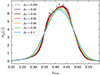 |
Fig. 3. Galaxy distribution observed through different Δz averaging as Eq. (70). The redshift convolution modifies the shape of the distribution for larger slicing compared to the real slicing as estimated with a very thin slicing (grey). For this case, all slicings Δz ≤ 0.06 produce a good estimate. |
3.5.3. Overall strategy
The uncertainty on the mean-z directly inferred with Eq. (69) would not fulfil the Euclid requirement Eq. (67). In doing this, we would be very conservative, allowing for any tomographic bin shape, whereas in reality, we know their shape a priori. Thus, we can define some priors on the np(z) properties to decrease the uncertainty. We describe two possibilities:
-
we assume a prior on the shape of the distribution, through a n(z) model;
-
we use Gaussian process formalism, to generate coherent realisations, assuming a kernel, which is related to how “fast” the distribution is evolving in redshift.
Thus in one case, we put a prior on the shape of the tomographic bin, and in the other, on the redshift variation.
3.5.4. Shifted-stretched model
For this approach, we evaluated a given model nmodel(z) with some parameters {p1, p2…}, by minimising the likelihood,
![Mathematical equation: $$ \begin{aligned} \ln \mathcal{L}&(\{p_1,p_2\ldots \}\vert n, \mathcal{C} _n)\nonumber \\&=-\frac{1}{2} \left[ n(z_i)-n^\mathrm{model}(z_i)\right]^\top \mathcal{C} _n^{-1}\left[ n(z_i)-n^\mathrm{model}(z_i)\right]\,, \end{aligned} $$](/articles/aa/full_html/2025/10/aa55551-25/aa55551-25-eq84.gif) (71)
(71)
where {np(zi)}i, and the associated covariance 𝒞n are the measured quantities. Then, using a Markov chain Monte Carlo9, the mean redshift and standard deviation were extracted from one thousand realisations of {nmodel}.
For the nmodel, we use the shifted-stretched model (SSM), which is commonly used for clustering redshifts; given a particular distribution n(z) with a mean redshift ⟨z⟩, two free parameters are used describing a redshift shift δz and a stretching s,
 (72)
(72)
This model is particularly convenient because for a given δz, s, the bias in mean redshift and standard deviation with respect to the model are δz and s. In our case, as the model is the true redshift distribution, we have
 (73)
(73)
 (74)
(74)
As we use the true redshift distribution of the bin as a model (simulation only), the performance may be overestimated compared to a realistic scenario, where the model is taken from a Self-Organised-Map estimate (e.g. Hildebrandt et al. 2021), or a candidate from a simulation (e.g. Gatti et al. 2018, 2022; Cawthon et al. 2022). That is why we also consider a more direct method.
3.5.5. Suppressed Gaussian process
We introduce the suppressed-Gaussian-process model (SGP) developed by Naidoo et al. (2023); GP reconstruction from clustering-redshifts was also performed in Johnson et al. (2017). The main benefit of this approach is that it is non-parametric. The procedure is as follows:
-
we generate realisations of Gaussian Process (GP) where the multivariate normal distributions are the measurements, and model the correlation between the points through a specific kernel10;
-
we apply to the realisations a suppression function that damps signals in regions where the measurements are consistent with zero;
-
the realisations are renormalised to unity;
-
the moments of the true distribution and their uncertainties are estimated from this large sample of normalised SGP realisations.
For the GP covariance, we chose a 3/2 Matern kernel function, and assume the length-scale l to be l = Δz/2 where Δz corresponds to the redshift slicing11. To validate these choices, we tested different kernels and length-scale, by comparing generated GP from discrete n(zi) and covariance to true n(z); see, for example, the right panel of Fig. 4.
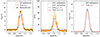 |
Fig. 4. Left: n(z) distribution measurement, with 50 associated GP realisations (orange), and the true distribution (red). Middle: SNR of the GP realisation (orange), and their convolution (blue). The SNR threshold ( = 3) is reported with the dashed line. Right: Associated SGP realisations, renormalised to unity (blue), compared to the true distribution (red). |
For the second step, given a GP realisation i, the associated SPG is
 (75)
(75)
where S is a suppression factor that removes the noisy part of the distribution. We chose the parametrisation
 (76)
(76)
In the above, the x variable is a smoothing of the continuous signal-to-noise ratio (SNR)
 (77)
(77)
Here 𝒢 is a Gaussian with a standard deviation Δz, * represents the convolution operation, which smooths the SNR between data points (and avoids non-physical cuts), and SNRthresh is the SNR threshold below which the suppressed factor is applied. Thus, if SNR < SNRthresh over a redshift range larger than Δz, the amplitude of the realisation nGPi(z) would be reduced by a factor k/3 × SNR. We fix k = 0.3 in Eq. (76), so that the suppressed factor rapidly drops for x < 1, but we ensured that the impact of this parameter was small.
In Fig. 4 we illustrate the whole procedure. We show for a measurement {np(zi)}i, 𝒞n (not normalised to unity), GP realisations, their SNR nGP/σ(z), and the associated normalised SGP realisations compared with the true distribution. It is clear that going from the left to the right panel, the overall procedure greatly improves the realisations. Nonetheless, the procedure could be optimised further in the future, since we did not rigorously explore all of the SGP parametrisation.
4. Results
In this section, we present the clustering-redshifts pipeline optimisation. In Fig. 5 we summarise the different ingredients entering the modelling of clustering redshifts, and the corresponding validation tests presented in this section. In Sect. 4.1, we describe the simulated data used. In Sect. 4.2, we compare the performance of the clustering estimator. In Sect. 4.3, we evaluate the hypothesis that the galaxy biases of cross-correlations and auto-correlations are the same at small scales. In Sect. 4.4, we determine the optimal scale range, and in Sect. 4.5, the optimal scale weighting. In Sect. 4.6, we test different spectroscopic slicing Δz for measurements affected by systematics, with the effects of these systematics tested individually in Sect. 4.7. In Sect. 4.8, we compare different galaxy bias correction methods. Finally, in Sect. 4.9, we investigate the impact of the tomographic bin definition on the redshift constraints.
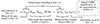 |
Fig. 5. Modelling the cross-correlation between spectroscopic samples in redshift slices and photometric bins, and reference to the corresponding tests we performed to optimise the pipeline. |
4.1. Investigation strategy
Our investigation strategy consists of varying a set of analysis parameters to check the impact on clustering redshifts. We chose to use three tomographic bins covering the full redshift range of interest and corresponding to different types of galaxies.
The three tomographic bins: “low-z”, “mid-z”, and “high-z”, were generated within the Flagship simulation with the photo-z cuts:
 (78)
(78)
 (79)
(79)
 (80)
(80)
They corresponds to bin 2, 7, and 10 in Fig. 1. For reference samples, we used BOSS LOWZ and CMASS, DESI ELG, and Euclid NISP-S like samples. We report the redshift distribution of the tomographic bins and spectroscopic samples in Fig. 1.
To characterise the uncertainty from sample variance in our analysis, we split each tomographic bin into five independent Flagship2 sky patches12 of 1000 deg2. As the simulation is limited to 5000 deg2, this is the maximum number of large independent patches that we can use. When investigating the optimal spectroscopic slicing we do not want our results to be biased because the points luckily cover the optimal part of the distribution. Thus, for every patch j = 1, …5, we varied the redshift slicing of the spectroscopic samples zi; Δz, by shifting the slice centres by j × Δz/5. To summarise, we tested over five independent 1000 deg2 sky patches for three tomographic bins, each cross-correlated with spectroscopic samples distributed into different slices for each patch (but with the same Δz).
4.2. Choice of the estimator weighting scheme
In this section, we compare the two different estimators of the angular correlation function, described in Sect. 3.4.1. We measured the auto-correlations of spectroscopic samples for a 1000 deg2 sky patch, a single redshift bin of width Δz = 0.05, and the two estimators:
-
 defined by Eq. (57), where weighting is applied to the ratio of pair counts;
 -
 defined by Eq. (58), where weighting is applied directly the pair counts.
Correlations were evaluated for the scale range 0.5– 5 Mpc, and with different weighting functions  . The results are reported in Fig. 6. We used logarithmic binning, and expect the measurements to be weighted by an effective function Weff ∝ rpγ + 2 (cf. Eq. (60)), which is confirmed by the matched amplitudes of blue-yellow and purple-red points. Importantly, we do not observe significant differences in the associated uncertainties between the two estimators with the corresponding weights. Given that the weighting variation does not offer any practical advantage, and leads to unnecessary complexity in the weighting process (cf. Appendix C), we adopted the first estimator, Eq. (57), as our fiducial choice for this analysis, and we will evaluate the optimal value of γ.
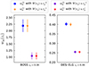 |
Fig. 6. Auto-correlations of two spectroscopic samples for a single redshift bin (Δz = 0.05). The yellow and red points are obtained using the first estimator |


4.3. Testing the bias-cancellation hypothesis
The scales used for clustering-redshifts calibration are typically very small [e.g. (0.1–5) Mpc] in order to minimise correlations between the calibration and the cosmological analysis, and to maximise the SNR. The associated nonlinear effects are often overlooked, however. Most authors assume that for two galaxy samples located within the same redshift bin, the two-point angular correlation function follows the relation:
 (81)
(81)
If we were using scalar product, instead of scale correlation function, this would be equivalent to the Cauchy–Schwarz equality, which implies that the density contrasts Δa and Δb are linearly dependent, and the Pearson correlation coefficient rab is 1, with
 (82)
(82)
At large scales (> 10 Mpc) galaxy samples act as linear tracers of the underlying dark matter density field. In this case, δa = bb/ba × δb, which means that galaxy field are linearly dependant. At smaller scales, the linearity between the dark matter field and galaxy statistics begins to break down. For a more complex biasing between matter field and galaxy field, however, we would still expect |rab|≤113.
At even smaller scales (within the one-halo regime), the modelling of galaxy fields as random variables of the dark matter field breaks down (e.g. in Swanson et al. 2008, clustering properties between galaxy subpopulations was investigated), potentially impacting cosmological inference (e.g. Chaves-Montero et al. 2023, in the context of weak lensing). We illustrate this issue with an extreme example: one sample consists only of central galaxies, whilst the other consists only of satellite galaxies. If we assume there is at most one satellite galaxy per halo, the auto-correlation of central and satellite galaxies would be very small on scales smaller than the halo size, but still non-zero as we are not evaluating 3d clustering. The positive cross-correlation between the two would be strong, however. This would result in rab ≫ 1, which is not possible for random variables. The reason for this discrepancy is that the statistics of the satellite distribution depend on those of the central galaxy distribution. In typical halo occupation distribution models, the probability of hosting a satellite galaxy is conditional on the presence of a central galaxy. Alternatively, if two galaxy samples populate different haloes, the cross-correlation would be very small on scales smaller than the halo size, while the auto-correlations would remain significant, leading to rab ≪ 1.
The scale range mentioned earlier (referred to as “small” and “smaller”), and the behaviour of the rab coefficients are not clearly known. We decided to improve this aspect for our Euclid calibration method.
The small-scale effects that we have described are not a hypothetical framework, as this type of behaviour has already been observed in spectroscopic surveys. For instance, the first DESI data provides clear evidence that LRGs and ELGs exhibit low cross-correlation signals at small scales (a phenomenon so-called “conformity”; Rocher et al. 2023; Yuan et al. 2025; Gao et al. 2024). This occurs because these galaxies reside in different haloes, with their properties influenced by the history of the halo.
Given that the under-correlation between red and blue galaxies is well established, we aimed to test whether the Flagship simulation could reproduce this small-scale effect. Our strategy was to split the two samples into redshift slices (Δz = 0.05) using true-redshift, and to measure the ratio with angular correlation,
 (83)
(83)
which is expected to be 1 under the linear approximation.
In Fig. 7 we show rab(rp, z) for the Flagship LRG and ELG-like samples. We recover the under-correlation at small scales, through rab(rp, z) < 1. This ratio not only decreases with scales, but also with redshift. Since the recovered n(z) is degenerate with r, an evolving r with redshift would introduce a bias in the reconstructed n(z). This confirms the presence of one-halo behaviour in the Flagship simulation. However, since these behaviours were only recently identified and are still being actively studied, it is likely that their implementation in the Flagship simulation is incomplete or not fully accurate. A thorough study of this aspect of the simulation and one-halo physics is beyond the scope of this article.
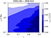 |
Fig. 7. Variation in the Pearson coefficients rab for Flagship LRGs with ELGs. This coefficient informs on the small-scale under-correlation of blue and red galaxies. |
In Fig. 8 we report rab(rp, z) for the three simulated photometric × spectroscopic bins (defined in Sect. 4.1). We observe significant scale and redshift evolution of the ratio, at least for the BOSS and DESI correlations, at scales smaller than 1 Mpc. Notably, we find r > 1, which we attribute to the physics of galaxy-halo connection and galaxy formation rather than non-linearities in the matter field (cf. the beginning of this subsection). Proving whether this is due to limitations in the HODmodelling or is a reliable prediction of the simulation is beyond the scope of our work. There is also a weak under-correlation for the low-z bin (and the mid-z) at scales (1–8) Mpc, but it does not appear to evolve with redshift, and is therefore not expected to introduce a bias into the n(z). This may correspond to the correction for non-linearities described above (r ≲ 1). For the high-z bin, we do not measure deviation from unity at any scale.
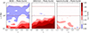 |
Fig. 8. Pearson coefficient for our three simulated bins: low-z, mid-z, and high-z. This term is assumed to be one for clustering-redshifts calibration. We see different behaviours, r = 1, r < 1, and r > 1 for different scales and redshifts, except for the high-z bin, for which r = 1 (almost) everywhere. |
Given these results, we are confident that using projected scales larger than 1.5 Mpc would avoid this one-halo effect14. As simulations improve in their modelling of galaxy halo properties, this test will need to be repeated. The ratio amplitude, scale, and redshift evolution are different depending on the tracers: under-correlation for DESI LRG and ELG in Fig. 7, and over-correlation for Euclid photo and DESI ELG in Fig. 8. We recommend to use only one type of spectroscopic tracer for the sample s when evaluating cross-correlations between photometric and spectroscopic samples at a specific redshift: wsp(zi), avoiding mixing ELGs and LRGs for example. If different spectroscopic tracers {sj}j are available for the same redshift zi, we can then predict different np(zi |sj) and combine them (e.g. Hildebrandt et al. 2021). Small-scale effect could lead to incompatibility as we show in this section, so that this procedure is more likely to detect systematics, and more robust.
4.4. Choice of the scale range
In this section, we investigate the best scale range that minimises the deviation
 (84)
(84)
while maximising the SNR. We explored a wide range of scales, including those previously discarded in Sect. 4.3. Unlike the estimator of w in Eq. (57), which averages over scales, our estimator was evaluated for a single scale15 as in Eq. (48). Consequently, we refer to the distribution measured as np (z | rp). We always normalised the measured distributions to unity. We employed three methods for correcting the bias, covering all the bias correction cases: no correction (i.e. M0), spectroscopic correction (i.e. M1), and full correction (i.e. M5)16. This approach allows us to assess how bias correction influences the optimal scale range.
We used three statistical indicators, as a function of the projected scale
-
the root mean square
![Mathematical equation: $$ \begin{aligned} \mathrm{RMS}[\Delta n]\,({r_{\rm p}}) = \sqrt{\frac{1}{N_z}\sum _{z_i} \Delta n\,(z_i\vert \, {r_{\rm p}}) ^2 }\,; \end{aligned} $$](/articles/aa/full_html/2025/10/aa55551-25/aa55551-25-eq103.gif) (85)
(85) -
the (mean) signal-to-noise-ratio
![Mathematical equation: $$ \begin{aligned} \mathrm{SNR}[n] ({r_{\rm p}}) = \frac{1}{N_z} \sum _{z_i} \frac{\vert n_{\rm p}(z_i)\vert }{\sigma _n (z_i)}\,; \end{aligned} $$](/articles/aa/full_html/2025/10/aa55551-25/aa55551-25-eq104.gif) (86)
(86) -
the reduced χ2
![Mathematical equation: $$ \begin{aligned} \chi _z^2({r_{\rm p}}) = \frac{1}{N_z} \left[\Delta n\,(z_i\vert \, {r_{\rm p}}\right]^\top _{z_i}\,\;\mathcal{C} _{n\vert {r_{\rm p}})}\;\left[\Delta n\,(z_i\vert \, {r_{\rm p}})\right]_{z_i}\,, \end{aligned} $$](/articles/aa/full_html/2025/10/aa55551-25/aa55551-25-eq105.gif) (87)
(87)
with Nz the number of points (equivalently the number of redshift slices of the spectroscopic sample). These indicators, evaluated at scales ranging from (0.05–10) Mpc for the different bins and bias corrections, are reported in Fig. 9. The thin lines represent individual realisations of 1000 deg2 patches, while the thicker lines indicate their means.
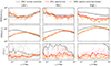 |
Fig. 9. RMS of Δn, SNR of n, and reduced χ2 of Δn (top to bottom) as a function of the projected scale rp for the three redshift bins (left to right) for three bias corrections (colours). The fine lines show five independent realisations of 1000 deg2, and the thick lines show their means. |
We first discuss the impact of the bias correction. Whilst the no-bias correction model M0 shows a higher SNR for scales lower than 1 Mpc, its corresponding χz2 value is very high, indicating that it is not accurate. Therefore, we focus exclusively on M1 and M5 for the remainder of this section. Both methods perform similarly for the SNR, but for mid-z and high-z, M5 provides a χz2 closer to unity.
For the three tomographic bins, the RMS is increasing for smaller scales. This increase is associated with a lower SNR, and the χz2 remains relatively constant. This suggests an overall consistency, and we can choose the scale range based on the SNR only. For the low-z bin, it peaks at 1 Mpc and then decreases. For the other two bins, it appears to peak around 2 Mpc, with a small decrease for larger scales.
In conclusion, the scale range (1.5–5) Mpc appears to be well suited for clustering redshifts; it is nearly optimal regarding the SNR; the χz2 is almost minimal for the whole range; it avoids the rp < 1.5 Mpc one-halo regime (excluded in Sect. 4.3); these scales are not used for cosmological analysis.
This scale range is the same as in Gatti et al. (2022) and Giannini et al. (2024), but significantly larger than in other works such as van den Busch et al. (2020), Cawthon et al. (2022), and Naidoo et al. (2023), which used scales of 0.1–1 Mpc h−1 or 0.5–1.5 Mpc h−1. Early clustering-redshifts studies even advocated for using smaller scales, down to the kpc range (Ménard et al. 2013; Schmidt et al. 2013). We note that we have chosen scales that avoid the one-halo term and the range of scales used for cosmology. One way to be conservative on the small-scales bias effects would be to use only large scales, overlapping those used in the 3 × 2 point analysis. In previous calibrations such as HSC, KIDS, and DES, scale choice was largely driven by the lack of spectroscopic sample (Hildebrandt et al. 2021), and the range was chosen to be at the peak of the SNR (Gatti et al. 2018). For Euclid, this will no longer be the case, and from Fig. 9 it is clear that larger scales can be used for calibration. However, it requires the generation of a more complex covariance to accurately propagate the correlation. This was proved to be informative through a Fisher formalism in Johnston et al. (2025), but never implemented in practice with simulated or real data, and is beyond the scope of thisarticle.
4.5. Choice of the scale weighting
In this section, we varied the weighting W(rp) in Eq. 53 and evaluated the RMS and SNR defined in Eqs. (85) and (86). The scale range was fixed to (1.5–5) Mpc following the last section’s conclusion. We tested three power laws
 (88)
(88)
and two different weighting schemes:
-
we scale-average the different correlation functions and compute their ratio, as in Eq. (53),
 (89)
(89) -
we scale-average the estimated n(zi| rp) as in Eq. (55),
 (90)
(90)
In Fig. 10 we show the comparison between the SNR and the RMS for the three tomographic bins, with three power laws, two weighting schemes, and two bias correction methods (M1 and M5). The small markers are the realisations for the five individual 1000 deg2 patches, while the larger markers indicate their means. The region of interest covers the lower right part of the plots, as it corresponds to minimum deviation and high SNR. Notably, the RMS/SNR plot displays a linear trend, indicating that points with a smaller deviation are associated with a better SNR, which is consistent with the expectations for an unbiased measurement. For all three redshift bins, the optimal weighting is the inverse scale weighting (darker red marker), a similar result to Schmidt et al. (2013) and Ménard et al. (2013). The reason is that SNR is higher, while RMS is lower, for scales around 1.5 Mpc than 5 Mpc (cf. Fig. 9). Ww and Wn are similar for the RMS, but the first performs slightly better for the SNR. These findings hold for M1 and M5. Additionally, we confirm that correcting the photometric bias for the first redshift bin is not strictly necessary in terms of RMS, but it does lead to abetter SNR.
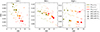 |
Fig. 10. SNR and RMS for the three tomographic bins (left to right), with three power laws as weighting functions (colours), two weighting schemes, and two bias-correction methods (M1 and M5). |
Thus, the best weighting scheme appears to be the inverse scale weighting applied to correlation functions, combined with a full bias correction approach.
4.6. Finding the optimal spectroscopic slicing
In the previous sections, we did not include systematics (e.g. magnification) in the measurement because we were questioning the optimal statistical choices on the two-point clustering itself, hence the use of statistical quantities such as RMS and SNR. In the rest of the article, we consider realistic measurements, including systematics, and evaluate their impact on the moments of the redshift distribution we aim to calibrate.
In this section, we varied the slicing of the spectroscopic sample Δz, cf. Sect. 3.2.2. On the one hand, narrow slices are more sensitive to corrections associated with bin modelling (cf. Sect. 3.2.3), magnification (cf. Sect. 3.1.4), or RSD (cf. Sect. 3.1.5). On the other hand, if the slices are too wide, there may not be enough points covering the distribution to properly measure the n(z), the shape would be flattened (cf. Sect. 3.5.2 and Fig. 3), and the assumption that galaxy biases and redshift distributions are constant may break (cf. Sect. 3.2.2). Therefore, we aim to find a compromise between narrow slices affected by systematic errors and large slices that are not statistically optimal, and for which the modelling might not be precise enough. The impacts of the systematic errors are tested one by one in the next Sect. 4.7.
We introduced the systematics using magnified sky coordinates and fluxes for the photometric and spectroscopic samples, and spectroscopic redshift (including peculiar velocity) for the spectroscopic sample. We used M5 as the bias correction method. For extracting the distribution moments from the {n(zi)} we employed the SGP n(z) reconstruction introduced in Sect. 3.5.5. We did so because, even with few points, fitting the true distribution (as with the SSM, cf. Sect. 3.5.4) is likely to yield good yet unrealistic results, whereas the SGP provides weaker yet realistic constraints.
We measured the mean (absolute) biases on the mean |⟨z⟩−⟨z⟩true| and standard deviation |σz/σztrue − 1| of the np(z) for different slicing, where the mean is evaluated over the five independent patches. We reported the mean values and their associated mean uncertainties in Fig. 11. We also created a similar plot using the SSM and obtain comparable results except for the uncertainties, which remain constant across the different slicing. This confirms our previous statement and justifies the choice of the SGP.
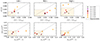 |
Fig. 11. Mean redshift and shape reconstruction with SGP, for the three tomographic bins. The different markers and colours are associated with different slicing Δz. The sandy region corresponds to the Euclid requirements, and the diagonal line shows a coherent deviation of 1σ. |
First of all, the uncertainties (y axis) on mean redshift and shape increase with the slicing Δz, and we also observe larger deviation for wider slices. Regarding the shape reconstruction (related to σz), narrow slices are not associated with larger deviations, except for the mid-z bin. For the mean redshift, small slicing is associated with similar or larger deviations than Δz ∼ 0.05, but not larger uncertainties. The optimum slicing appears to correspond to 0.04 ≤ Δz ≤ 0.06.
Consequently, we decided to use a redshift slicing of Δz = 0.05 for every bin, for the rest of the study. This is larger than the slicing used for DES (Gatti et al. 2022; Giannini et al. 2024), but the same as the previous Euclid clustering-redshifts paper (Naidoo et al. 2023). As illustrated by the sandy region in Fig. 11, we predict that the systematic errors for this redshift slicing will not shift the data points outside the Euclid requirement. Since the Δz = 0.05 points are predominantly on the diagonal (except for the mid-z mean-z), this suggests that the corrections are fairly small for this slicing: the parameters are not biased more than 1σ away from the truth. The mid-z is the only case where we might fail to fulfil the requirement if we do not correct for the systematic errors. We investigated the origin of this deviation in detail in the next section.
4.7. Evaluating the (mis-)modelling of the clustering, magnification, and RSD
For clustering redshifts, we measure the cross-correlation of a wide photometric tomographic sample with several spectroscopic slices, and we assume that only the photometric galaxies within the redshift range of the spec-z cuts contribute to a non-zero correlation. There can be three corrections:
-
galaxies in the nearby redshift (nearby bins) can correlate as well (we refer to this as the one-bin approximation);
-
galaxies not covering the same redshift range can be correlated through magnification processes;
-
spectroscopic redshifts can be different than true redshifts, leading to correction on the ns at the boundary of the bin.
Two of these effects can be understood as bin border effects, and for larger slices they are expected to decrease in proportion. For wide spectroscopic slices, the assumption that n(z) and b(z) are constant within the bin might break down. We also note that spectroscopic interlopers were not included in the Euclid spectroscopic samples.
In the previous Sect. 4.6, we demonstrated that the compromise between having enough points np(zi) and limiting these effects, corresponds to slicings Δz = 0.04–0.06, regardless of the tomographic bin. To assess the influence of each effect, we used the idealised bias correction M5 to avoid the impact of galaxy bias, and proceed as follows:
-
To test the impact of the one-bin approximation, we compared the cross-correlation wsp(zi) with spectroscopic slices and the tomographic bin for two cases. In the first one, referred to as the “full bin”, the photometric sample is the fiducial one used in this paper. For the second case, referred to as the “independent bins”, we used idealised tomographic bins. To generate these idealised tomographic bins, for every zi, we keep only the photometric galaxies within the same redshift range as the spectroscopic galaxies (using true-z), and then complete this sample with randoms to maintain the total number of galaxies as in the full tomographic bin. This ensures that only the galaxies within the redshift slice of the spectroscopic sample contribute to the correlation, for each spectroscopic slice.
-
To test the magnification effect, we compared the results using the magnified variables for position and fluxes (over which we apply the samples cuts), or the unmagnifiedones.
-
To test the RSD effect, for the spectroscopic samples we used either the Flagship true redshifts, or the observed ones, the latter corresponding to a spectroscopic-like redshift estimate (including velocities).
-
We also tested all these effects together, referred to as “Total”.
In Fig. 12 we show the deviations associated with the different systematic effects for different slicing, for the SGP. The same test for SSM methods is presented in Fig. 13. The corresponding values for the two procedures are listed in Table D.1 for Δz = 0.05, in Appendix D. For RSD and magnification, we have to consider the full tomographic bin, which by default comes with the one-bin approximation. Therefore, the full bin assumption has to be compared with “independent bins”, and the RSD or magnification has to be compared with the full bin.
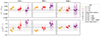 |
Fig. 12. Deviations on the mean-z (top) and standard deviation (bottom), with SGP fitting, for the three tomographic bins (left, middle, and right), with three Δz slicings (colours) and different implemented systematic effects (marker). The shadowed bands correspond to the Euclid requirement on both parameters. The dark and light error bars indicate 68.3% and 95.5% uncertainties |
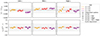 |
Fig. 13. Same as Fig. 12 for the two parameters of the SSM model, which are equivalent to ⟨z⟩−⟨z⟩true and σz/σztrue − 1. |
For the SSM and SGP, with Δz = 0.05, the constraints on the redshift standard deviation σ are within the requirements independently from the effects. Only a large slicing of Δz = 0.08 leads to some measurements out of the requirements because not enough points cover the distribution, and with larger slicing, the distribution appears flattened (σz/σztrue > 1) as shown in Fig. 3.
Regarding the mean redshift bias, all the “independent bin” measurements are consistent with no deviation at the 1 to 2σ level with the SGP and SSM. This suggests that our choice of scale and weighting is sufficient to limit the small-scale effects (cf. Sect. 4.4). In general, for the three tomographic bins, all the systematics lead to some deviations compared to the independent bins, but distinguishing these variations from statistical fluctuations is complicated. It is clear that the SGP procedure is more sensitive to these effects. The reason for this is that with SSM we compare the measurements with a model free from these effects. As this model is, in our case, the truth, its results may be optimistic. Nevertheless, with a SOM estimate as a model, we might expect a similar low sensitivity to these effects. For smaller bin sizes, the error bars are smaller, but the deviation due to systematic effects is at least as large as for other sizes. Wider slices are associated with greater uncertainty, and the balance between accuracy and precision is achieved for Δz = 0.05. For this bin size, the systematic effects do not produce deviations that exceed the requirements. However, for the mid-z bin, with SGP these systematic effects result in a deviation right at the limit of the budget on the mean-z, as the bias is 0.0038 ± 0.0017 (the requirements being 0.0038). For the optimistic case (SSM), the deviation remains within the requirements: the bias in mean redshift being 0.0022 ± 0.008. The effect causing this large deviation for SGP seems to be the one-bin approximation.
In Fig. 14, we report the true redshift distribution of three bins are shown alongside clustering-redshifts measurements for three slicing values: Δz = 0.02, 0.05, and 0.08, excluding the effects of RSD and magnification. We observe increasing deviations with finer slicing, whilst the shape reconstruction becomes less precise for coarser slicing (cf. Fig. 3). The small slicing deviations are higher for the mid-z and high-z bin, as one can expect since η± increase with redshift. We also see that large slices lead to worst shape estimate for the low-z bin, as its width is narrower.
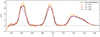 |
Fig. 14. True-redshift distributions of tomographic bins in black, and the clustering-redshifts measurements with M5 for three spectroscopic slicings: Δz = 0.02, 0.05, 0.08 (orange, red, and purple). |
In Appendix E we explore an alternative modelling including correlation with neighbours slices ( cf. Sect. 3.2.3). In short, despite our effort we did not manage to improve the accuracy of the modelling with extra-terms.
4.8. Comparison of the different bias-correction methods
In this section, we explore the different possibilities for breaking the degeneracy between np(z) and bp bs from wsp (cf. Eq. (47)). In the first subsection, we focus on measuring the photometric bias alone, since this is the challenging aspect.
4.8.1. Measuring the photometric galaxy bias evolution
In Sect. 3.3.2, we proposed to improve existing photometric bias corrections (van den Busch et al. 2020; Cawthon et al. 2022) with two methods to measure bp(z), applicable to real data, specifically for photometric galaxies with zphoto < 1.6 (i.e. fully covered by spectroscopic samples). The larger binning method M3 is applied in Fig. 15 and the smaller binning method M4 is applied in Fig. 16. They are represented by orange dashed lines. For both figures we also include the results using either the partial correction (blue dashed) or width correction (green dashed), for comparisons with previous analyses (van den Busch et al. 2020; Cawthon et al. 2022; Giannini et al. 2024). Additionally, we present the best fit degree-3 polynomial for the partial and the full corrections (solid lines) from a standard χ2 minimisation. The grey line shows the measurement using true-z, which we want to recover after the corrections.
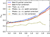 |
Fig. 15. True wpp for Δz = 0.05 in grey and measurement with corrections factors including M3 as dashed green, blue, and orange lines for photo-z binning Δz = 0.1. The best fits from degree-3 polynomials are reported with solid lines. The wpp used for M3 is the best-fit model of the full correction (solid red line). |
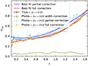 |
Fig. 16. Same as Fig. 15, but for M4, with a smaller photo-z binning Δz = 0.02. The wpp used for M4 is the best-fit model of the full correction (solid red line). |
We find that assuming the photo-z as the true-z (width-only correction), neither the amplitude nor the redshift evolution is well measured. For the partial correction, whilst the redshift evolution appears well-recovered, differences in amplitude persist. Finally, our full correction method significantly outperforms the others: in both figures, we recover the amplitude and redshift evolution of the bias more accurately. Notably, the bias evolves weakly for z < 1, suggesting that correcting the photometric bias at low redshift may not be necessary.
Since the partial and full corrections both give a good trend for the redshift evolution of the galaxy bias, one could argue their performance are identical in the context of clustering redshifts, as the measured np(z) can always be latterly renormalised. With the correct amplitude for the galaxy bias, evaluating whether the np(z) measured is directly normalised to unity can provide valuable information. Deviations from unity could indicate
-
a contamination from systematics, such as the small scale effect illustrated in Sect. 4.3;
-
the photometric sample is not fully covered by spec (and what is the fraction);
-
a problem with the spectroscopic redshifts, such as interlopers.
In that sense, the full correction performs significantly better than the partial one. The performance of our bias measurement may depend on the specific photo-z code and the quality of the available photometry, and data implementation will have to address this question.
4.8.2. Comparison of the methods
In this section, we compare the different bias correction methods introduced in Sect. 3.3.1, including M3 and M4. We aim to evaluate the bias correction performance, thus we work in an idealised framework with independent bins, no RSD, and no magnification (i.e. the “independent bin” test of Sect. 4.7). We employ a redshift slicing Δz = 0.05. We report in colours the deviations on the mean redshift and standard deviation for the six methods M0–M5, in Figs. 17 (for SSM) and 18 (for SGP). For each method, we have five realisations by varying the sky patch. We also give the values for the biases on mean-z and standard deviation in Table D.1, in Appendix D.
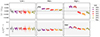 |
Fig. 17. Deviations with the SSM fitting on the mean redshift (upper panel) and standard deviation (lower panel) for the six methods M0–M5 in colour, for five sky patches (same colour). The requirements are represented by the shaded area. The dark and light error bars indicate 68.3% and 95.5% uncertainties. |
We can see that at low-z it is not necessary to correct for the photometric bias, and spectroscopic correction M1 produces good estimates. At mid-z it is necessary to correct at least for the spectroscopic bias, and ideally for both with M3 or M4. At high-z, it is essential to correct both biases. We observe that M3 performs significantly better than M4 for SSM and SGP; indeed, the redshift evolution is better captured in Fig. 15 than in Fig. 16. This difference may be attributed to the fact that smaller slices are more sensitive to systematic effects, as discussed in Sect. 4.6. Overall, M3 performs similarly to the idealistic M5 and is consistently the best bias correction method, exhibiting performance akin to M1 for low-z (though with slightly larger errorbars).
In conclusion, using M3 for every bin yields unbiased estimates of the mean redshift and standard deviation across all bins, with uncertainties that fall within the requirements for both methods. The values presented in these two figures are reported in Table D.2.
4.9. Tomographic bin uncertainties
We defined the tomographic bins as equi-populated, based on the assumption that the uncertainty scales with the total number of galaxies in each bin. For the 10 spectroscopic samples, we used 1-DESI-BGs, 2-BOSS, 3-DESI-LRGs, 4-DESI-LRGs, 5-DESI-LRGs, 6-DESI-ELGs, 7-DESI-ELGs, 8-Euclid-NISP, 9-Euclid-NISP, 10-Euclid-NISP.
In Fig. 19 we plot in red the uncertainty on the mean redshift σ(⟨z⟩) for every tomographic sample, and its standard deviation σ(σ(⟨z⟩)), evaluated for the five 1000 deg2 sky-patches with jackknife covariance, with SSM fitting. Interestingly, we find that the uncertainty is not constant. It remains the same for the first two samples, then decreases across the next six samples, before increasing again for the final ones. We also report for the first two samples, the case of 2500 deg2 sky patches in dark red, and observe a mean-z uncertainty reduction of 40%.
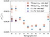 |
Fig. 19. Uncertainties on mean-z with SSM fitting for five sky realisations in red. We also plot the best-fit uncertainty model in blue. |
McQuinn & White (2013) predicted that “the linear bias times number of objects in a redshift bin generally can be constrained with cross-correlations to fractional error  ”, where NΔz is the number of spectroscopic redshift slices, and Ns the number of spectroscopic galaxies17. This expression describes how well the redshift distribution can be measured, whereas we are primarily interested in its moments. We assume that, at first order, the scaling should behave similarly, but with a different coefficient, which is complicated to predict because of the complexity of the mean-z fitting procedure. As a consequence, the uncertainty should depend on the number of spectroscopic galaxies, rather than on the volume or the number of photometric galaxies. However, for the low-z bins, the spectroscopic density is sufficiently high, especially with DESI-BG-like sample, that we might enter a cosmic variance (CV) regime. In this case, uncertainties are no longer sample-dominated (i.e. the shot noise 1/ns is subdominant). Thus, we introduce a maximum spectroscopic density to reach the cosmic variance limit ncv, which in principle depends on z, but that we assume to be constant. Our uncertainty model is
 (91)
(91)
where A is a constant independent of the tomographic bin, and VTB is the volume of the tomographic bin.
The equation above also indicates that the uncertainty scales with the inverse of the square root of the tomographic volume. This explains why in Fig. 8 of Naidoo et al. (2023), the uncertainty scales as a power law of the survey area Aγ, and the best-fit power law is close to γ = −1/2.
We constrained the A and ncv coefficients with the set of tomographic bin measurements using a χ2 procedure, and report in Fig. 19 the best-fit model in blue for 1000 and 2500 deg2. We observe a good agreement, particularly given that we neglected complications arising from galaxy biases and the mean-redshift fitting procedure. The uncertainty is largest for the low-z tomographic bins where the survey volume is much smaller and precision is limited by the CV regime. For the high-z samples, the uncertainty increases due to the reduced density of spectra, which is not sufficiently offset by the larger volume. The best-fit ncv roughly corresponds to the DESI-BGS density divided by a factor of four (and the BOSS density by a factor of 1.8), and it only plays a role for the first two bins.
As a result, to achieve consistent uncertainty across bins with clustering-z, the tomographic bin definition would need to be adjusted according to an uncertainty model like Eq. (91). However, the tomographic bin definition is primarily influenced by cosmological constraining power (e.g. Euclid Collaboration: Pocino et al. 2021), and our results alone do not provide sufficient grounds to recommend a change in binning strategy. However, the precision of the mean redshift is one of the key limiting factors in cosmic shear analyses (see, e.g., Reischke 2024), and the impact of bin definitions on the accuracy of redshift calibration is often overlooked.
5. Application to the ten Euclid tomographic bins
In this section, we applied our pipeline to calibrate the ten tomographic bins described in Sect. 2.2. For the spectroscopic samples, following our recommendation (see Sect. 4.3) we only correlated a tomographic bin with one spectroscopic tracer at a time. We used the following tracers for the different bins: 1-DESI-BGs, 2-BOSS, 3-DESI-LRGs, 4-DESI-LRGs, 5-DESI-LRGs, 6-DESI-ELGs, 7-DESI-ELGs, 8-Euclid-NISP, 9-Euclid-NISP, 10-Euclid-NISP. For simplicity, we did not consider the joint constraint of several spectroscopic tracers covering the same bin, which would provide additional information. For each bin, we produced several independent realisations by selecting distinct patches in Flagship 2. For the first two tomographic bins, we generated two 2500 deg−2 patches, while for the remaining eight bins, we used five 1000 deg−2 patches. This approach ensures similar uncertainties across bins, as explained in Sect. 4.9.
The true tomographic bin distribution, and the clustering-redshifts measurements are reported in Fig. 20. The measurements are visually indistinguishable from the truth. To quantify how good they are, we show the (optimistic) SSM calibration of the mean-z and standard deviations in Fig. 21. The results with the conservative SGP calibration are shown in Fig. 22. For comparison, we also plot the previous results of Naidoo et al. (2023) for the mean redshift (with Flagship1 samples). Our results using the SSM method are fully successful; for every bin and patch realisation, we meet the Euclid requirements for the mean redshift and shape, unlike prior results. However, as expected, the "conservative" SGP method yields larger uncertainties and deviations. In particular, for some bins (especially bins 1, 3, and 7), we observe slightly larger deviations and uncertainties than allowed by the mean redshift requirement. We tested the effect of increasing the patch sizes by a factor of two and found that the mean-z bias was reduced on average by 40%, which was sufficient to meet the requirement for all bins.
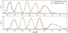 |
Fig. 20. True-redshift distribution of the simulated Flagship2 ten tomographic bins with zp < 1.6 (solid lines) and their clustering-redshifts measurements with our pipeline, including all systematics and realistic bias correction M3. The first two bin measurements are realised with 2500 deg2 sky patches, and the other eight are realised with 1000 deg2 sky patches. The dark and light error bars indicate 68.3% and 95.5% uncertainties, but are barely visible by eye. |
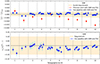 |
Fig. 21. Deviations in the mean redshift (top) and the redshift standard deviation (bottom) for the ten Flagship2 tomographic bins relative to the true-redshift distributions using the SSM method. The deviations are shown for each bin and sky patch. We consider patches of 2500 deg2 for the first two bins, and 1000 deg2 for the others. The Euclid requirements on the uncertainty are highlighted by the shaded area centred around zero. The uncertainties are consistent across all the bins for the mean redshift and we achieve a clear improvement from previous work shown in red. For the redshift standard deviations, the uncertainties are slightly underestimated, but this is within an acceptable range given the requirements. |
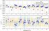 |
Fig. 22. Deviations in the mean redshift (top) and the redshift standard deviation (bottom) using the SGP method for the same bin configuration as in Fig. 21. The Euclid requirements on the uncertainty are highlighted by the shaded area centred around zero. For some bins (particularly bins 1, 3, and 7), we observe slightly larger deviations and uncertainties than permitted on the mean redshift. However, a clear improvement compared to previous work (shown in red) is still evident. The redshift standard deviations are unbiased and fall within the required range (shaded sandy area). |
Part of the improvement to Naidoo et al. (2023) is due to the use of a larger cosmic volume with Flagship2 instead of Flagship1. Nevertheless, with our pipeline we also got significantly lower mean redshift biases than Naidoo et al. (2023). The main differences between our pipeline and the previous one are our estimator (cf. Sect. 4.2), the scale range (cf. Sect. 4.4), the measurements being evaluated for each spectroscopic tracer (cf. Sect. 4.3), the bias correction method (cf. Sect. 4.8), and some improvement in the implementation of SSM and SGP (cf. Sect. 3.5). We note that we did include the effect of magnification contrary to Naidoo et al. (2023). In conclusion, we predict that clustering-redshifts will be able to satisfy the Euclid requirements.
6. Conclusion
We optimised and evaluated the performance of the clustering-redshifts method for calibrating the redshift distributions of Euclid tomographic bins.
Using the Flagship2 simulation, we generated realistic spectroscopic and photometric mock samples based on BOSS, DESI, and Euclid. The photometric sample was divided into ten equally populated tomographic bins, with a maximum photo-z of 1.6. We used up to five 1000 deg2 patches to fully exploit the volume of the simulation.
We measured the angular auto- and cross-correlations of these samples under various methodological choices and investigated alternative approximations to model the clustering.
From these clustering measurements, we calibrated the redshift distributions via two distinct methods. One method involved fitting the data points using a model n(z| p1, …) with free parameters. In practice, a complementary calibration, such as the self-organising map can be used to define the model (e.g., Hildebrandt et al. 2021; Gatti et al. 2022). The other method relies on Gaussian processes to directly fit the data without assuming a specific model. With the latter, the SOM and clustering-redshifts calibrations can both be run independently, or be combined as in the case of DES (Myles et al. 2021; Gatti et al. 2022).
In Sect. 4 we investigated and concluded the following about the clustering-redshifts technique and angular clustering.
-
In Sect. 4.2 we argued that the integrated pair-count estimator w(1) is a better choice than w(2) for measuring the integrated clustering (i.e. integrating the ratio DD/RR instead of taking the ratio of the integrated DD and RR).
-
In Sect. 4.3 we explained a potential issue with very small scales that arises from the one-halo properties of the clustering. We concluded that scales should always be larger than 1.5 Mpc to limit this problem. We also recommended separating the clustering-redshifts measurements for the different spectroscopic tracers.
-
In Sects. 4.4 and 4.5, we ran an optimisation of the scale range choice and weighting. With the Flagship simulation, we achieved a good compromise with 1.5 < rp < 5 Mpc with an inverse scale weighting.
-
In Sect. 4.6 we showed that the optimal spectroscopic slicing given our tomographic bins and the different systematics was Δz ≈ 0.05.
-
In Sect. 4.7 we showed that approximating ∫dz n2(z)⋯ (Limber-full-z) with some n2(zi)∫dz⋯ expressions (Limber-1-bin) is the main systematic effect and that magnification has some limited impact on the np(z) inference.
-
In Sect. 4.8 we compared different bias corrections and introduced a way to measure the photometric galaxy bias by splitting the TB into smaller bins and interpolating these effective biases over redshift (i.e. M3). The results of this method were comparable to the ideal case M5, in which photometric bias is measured using true redshifts. It should be used as the fiducial correction scheme.
-
Finally, we investigated in Sect. 4.9 the dependence of the mean-z error bars on the clustering-redshifts parameters, and confirmed that they are mainly driven by the number of spectroscopic galaxies that is available in the footprint.
In Sect. 5 we applied the optimised pipeline to calibrate the Euclid simulated tomographic bins. The calibration performance using the SSM model met or exceeded the required accuracy, while the SGP method yielded comparable results, but they were slightly below the requirements in certain cases. It is important to note that these results were derived from limited sky patches with correction methods that can still be improved in future work. These results represent a significant improvement over the previous Euclid clustering-redshifts study (Naidoo et al. 2023) overall and demonstrated that the clustering-redshifts technique is robust.
Additionally, as discussed in Sect. 2, we assumed that the H α sample had a purity of 100%. In reality, however, when we bin the sample into small redshift intervals, we expect that some of these galaxies may be interlopers, that is, they might be located at different redshifts due to noise or a misidentification of a spectral lines. This situation might significantly impact clustering-redshifts measurements because photometric galaxies at a similar redshifts as the interlopers would contribute to the clustering signal, which would bias the inferred n(z). It is therefore crucial to determine the fraction of these interlopers and their redshift distribution to correct for this effect. The clustering-redshifts technique can indeed be used to constrain the properties of interlopers by cross-correlating the NISP sample with other spectroscopic data or with photometric data with priors on their n(z).
As already mentioned in Sect. 4.3, the galaxy-halo connection implemented in the Flagship simulation might not be accurate, and our statistical estimator might be optimistic. It might therefore still be beneficial to use larger scales even though they are not statistically optimal. These larger scales will be used for the 3 × 2 analysis, which necessitates the generation of a more complex covariance to accurately propagate the correlation with the calibration (e.g. the work of Johnston et al. 2025). Although this approach is more complicated, the advantage is that the distribution would be free of small-scale potential bias, which may prove worthwhile.
Finally, we restricted the calibration to galaxies with a maximum photo-z of 1.6 because we lack dense spectroscopic samples above redshift 1.8, which sets a strict upper limit. Clustering-z for HSC, KIDS, and DES was even more limited than Euclid, with a maximum redshift of z ∼ 1. In the far future numerous spectroscopic samples from Lyman-break galaxies are expected to be observed by spectroscopic experiments such as DESI-II, MUST, and WST (if funded). In a much shorter time frame, QSOs might be used one could utilise QSOs to cover the redshift range 1.5 < z < 3. These constraints alone would most likely not fulfil the Euclid requirements because QSOs have a low-density, however, but they would still provide valuable information.
In the linear regime, RSD contribute to the projected galaxy density contrast through the apparent large-scale flow, of galaxies across the redshift boundaries of the samples. The redshift z we use to parametrise the D and μ terms includes the peculiar velocity, and is referred to as observed redshift.
Our Universe and its observation is assumed to be isotropic. Although the real isotropy of our Universe seems a reasonable hypothesis, observation may not always support it. For example, closer to the Galactic plane, there is more star contamination, leading to angular anisotropy. The Euclid observation strategy might also induce some angular anisotropy. This could potentially introduce bias on the cosmological parameters, especially for experiments such as Euclid or LSST (Baleato Lizancos & White 2023). Indeed, clustering-redshifts may be a valuable tool to investigate this issue by splitting the samples into independent sky patches.
The magnification of the two samples by the lower-z matter is negligible as it is a smaller correction (μ × μ cf. Sect. 3.1.2).
Positive convergence is induced by galaxy over-density. Correlation with voids would probe the negative convergence regime.
For scales that are neither too small nor too large, it should be a valid hypothesis, at least to first order.
Of course, in practice, all the previous integrals are discrete, with
 (63)
(63)
We use the python package emcee (Foreman-Mackey et al. 2013).
We use the python package Georges (Ambikasaran et al. 2015).
The length-scale represents the characteristic distance over which the function values are correlated.
We applied cuts on the RA coordinates, with a width of ΔRA = 17.5 deg.
As shown in Appendix A for quadratic non-linearities (second-order effects), we expect rab ≈ 1, with the correction arising from third-order terms. Pushing further the perturbative development, we can show that indeed rab ≤ 1, analogously to the Cauchy–Schwarz inequality.
We note that we are using angular correlation, so most of the 3-D separation between galaxies is much larger than this 1.5 Mpc.
In practice, it is evaluated for a small scale bin.
We expect the results with M2-3-4 to be similar to that of M5.
We have slightly adjusted the convention to remain consistent with the rest of our article.
There are different and confusing conventions in the literature. For instance, sometimes α is given as s, 2.5s, or 5s − 2.
Acknowledgments
The authors thank Alex Alarcon, Carles Sánchez, Elisa Chisari, and Santi Ávila for enlightening discussions, as well as Krishna Naidoo for his help, code, and results sharing. The authors also acknowledge Mathias Urbano for his code support. This work was supported by the MICINN projects PID2019-111317GB-C32, PID2021-123012NB-C41, PID2022-141079NB-C32, CNS2023-144328 (Carteu) as well as predoctoral program AGAUR-FI ajuts (2024 FI-1 00692) Joan Oró. IFAE is partially funded by the CERCA program of the Generalitat de Catalunya. This work has made use of CosmoHub, developed by PIC (maintained by IFAE and CIEMAT) in collaboration with ICE-CSIC. It received funding from the Spanish government (grant EQC2021-007479-P funded by MCIN/AEI/10.13039/501100011033), the EU NextGeneration/PRTR (PRTR-C17.I1), and the Generalitat de Catalunya. The Euclid Consortium acknowledges the European Space Agency and a number of agencies and institutes that have supported the development of Euclid, in particular the Agenzia Spaziale Italiana, the Austrian Forschungsförderungsgesellschaft funded through BMIMI, the Belgian Science Policy, the Canadian Euclid Consortium, the Deutsches Zentrum für Luft- und Raumfahrt, the DTU Space and the Niels Bohr Institute in Denmark, the French Centre National d’Etudes Spatiales, the Fundação para a Ciência e a Tecnologia, the Hungarian Academy of Sciences, the Ministerio de Ciencia, Innovación y Universidades, the National Aeronautics and Space Administration, the National Astronomical Observatory of Japan, the Netherlandse Onderzoekschool Voor Astronomie, the Norwegian Space Agency, the Research Council of Finland, the Romanian Space Agency, the State Secretariat for Education, Research, and Innovation (SERI) at the Swiss Space Office (SSO), and the United Kingdom Space Agency. A complete and detailed list is available on the Euclid web site (https://www.euclid-ec.org/).
References
- Adame, A. G., Aguilar, J., Ahlen, S., et al. 2024, AJ, 167, 62 [NASA ADS] [CrossRef] [Google Scholar]
- Addison, G. E., Bennett, C. L., Jeong, D., Komatsu, E., & Weiland, J. L. 2019, ApJ, 879, 15 [NASA ADS] [CrossRef] [Google Scholar]
- Ambikasaran, S., Foreman-Mackey, D., Greengard, L., Hogg, D. W., & O’Neil, M. 2015, IEEE Trans. Pattern Anal. Mach. Intell., 38, 252 [Google Scholar]
- Baleato Lizancos, A., & White, M. 2023, JCAP, 07, 044 [Google Scholar]
- Behroozi, P. S., Wechsler, R. H., & Wu, H.-Y. 2013, ApJ, 762, 109 [NASA ADS] [CrossRef] [Google Scholar]
- Blas, D., Lesgourgues, J., & Tram, T. 2011, JCAP, 07, 034 [CrossRef] [Google Scholar]
- Bordoloi, R., Lilly, S. J., & Amara, A. 2010, MNRAS, 406, 881 [NASA ADS] [Google Scholar]
- Campos, A., Yin, B., Dodelson, S., et al. 2024, ArXiv e-prints [arXiv:2408.00922] [Google Scholar]
- Carretero, J., Tallada, P., Casals, J., et al. 2017, in Proceedings of the EuropeanPhysical Society Conference on High Energy Physics. 5-12 July, 488 [Google Scholar]
- Cawthon, R., Elvin-Poole, J., Porredon, A., et al. 2022, MNRAS, 513, 5517 [NASA ADS] [CrossRef] [Google Scholar]
- Chaves-Montero, J., Angulo, R. E., & Contreras, S. 2023, MNRAS, 521, 937 [Google Scholar]
- Chisari, N. E., Alonso, D., Krause, E., et al. 2019, ApJS, 242, 2 [Google Scholar]
- Contarini, S., Verza, G., Pisani, A., et al. 2022, A&A, 667, A162 [NASA ADS] [CrossRef] [EDP Sciences] [Google Scholar]
- Davis, M., & Peebles, P. J. E. 1983, ApJ, 267, 465 [Google Scholar]
- Davis, C., Rozo, E., Roodman, A., et al. 2018, MNRAS, 477, 2196 [Google Scholar]
- Dawson, K. S., Schlegel, D. J., Ahn, C. P., et al. 2013, AJ, 145, 10 [Google Scholar]
- DESI Collaboration (Aghamousa, A., et al.) 2016, ArXiv e-prints [arXiv:1611.00037] [Google Scholar]
- Elvin-Poole, J., MacCrann, N., Everett, S., et al. 2023, MNRAS, 523, 3649 [NASA ADS] [CrossRef] [Google Scholar]
- Eriksen, M., Alarcon, A., Cabayol, L., et al. 2020, MNRAS, 497, 4565 [CrossRef] [Google Scholar]
- Euclid Collaboration (Blanchard, A., et al.) 2020, A&A, 642, A191 [NASA ADS] [CrossRef] [EDP Sciences] [Google Scholar]
- Euclid Collaboration (Desprez, G., et al.) 2020, A&A, 644, A31 [EDP Sciences] [Google Scholar]
- Euclid Collaboration (Ilbert, O., et al.) 2021, A&A, 647, A117 [NASA ADS] [CrossRef] [EDP Sciences] [Google Scholar]
- Euclid Collaboration (Pocino, A., et al.) 2021, A&A, 655, A44 [NASA ADS] [CrossRef] [EDP Sciences] [Google Scholar]
- Euclid Collaboration (Castander, F., et al.) 2025, A&A, 697, A5 [Google Scholar]
- Euclid Collaboration (Cropper, M., et al.) 2025, A&A, 697, A2 [Google Scholar]
- Euclid Collaboration (Jahnke, K., et al.) 2025, A&A, 697, A3 [Google Scholar]
- Euclid Collaboration (Le Brun, V., et al.) 2025, A&A, submitted [Google Scholar]
- Euclid Collaboration (Mellier, Y., et al.) 2025, A&A, 697, A1 [Google Scholar]
- Foreman-Mackey, D., Hogg, D. W., Lang, D., & Goodman, J. 2013, PASP, 125, 306 [Google Scholar]
- Gao, H., Jing, Y. P., Xu, K., et al. 2024, ApJ, 961, 74 [Google Scholar]
- Gatti, M., Vielzeuf, P., Davis, C., et al. 2018, MNRAS, 477, 1664 [Google Scholar]
- Gatti, M., Giannini, G., Bernstein, G. M., et al. 2022, MNRAS, 510, 1223 [Google Scholar]
- Giannini, G., Alarcon, A., Gatti, M., et al. 2024, MNRAS, 527, 2010 [Google Scholar]
- Gwyn, S., McConnachie, A. W., Cuillandre, J. C., et al. 2025, ArXiv e-prints [arXiv:2503.13783] [Google Scholar]
- Hartlap, J., Simon, P., & Schneider, P. 2007, A&A, 464, 399 [NASA ADS] [CrossRef] [EDP Sciences] [Google Scholar]
- Hartley, W. G., Chang, C., Samani, S., et al. 2020, MNRAS, 496, 4769 [Google Scholar]
- Hildebrandt, H. 2016, MNRAS, 455, 3943 [NASA ADS] [CrossRef] [Google Scholar]
- Hildebrandt, H., van den Busch, J. L., Wright, A. H., et al. 2021, A&A, 647, A124 [EDP Sciences] [Google Scholar]
- Huterer, D., Takada, M., Bernstein, G., & Jain, B. 2006, MNRAS, 366, 101 [Google Scholar]
- Jarvis, M. 2015, Astrophysics Source Code Library [record ascl:1508.007] [Google Scholar]
- Johnson, A., Blake, C., Amon, A., et al. 2017, MNRAS, 465, 4118 [Google Scholar]
- Johnston, H., Elisa Chisari, N., Joudaki, S., et al. 2025, A&A, 699, A127 [NASA ADS] [CrossRef] [EDP Sciences] [Google Scholar]
- Krause, E., Fang, X., Pandey, S., et al. 2021, ArXiv e-prints [arXiv:2105.13548] [Google Scholar]
- Landy, S. D., & Szalay, A. S. 1993, ApJ, 412, 64 [Google Scholar]
- Laureijs, R., Amiaux, J., Arduini, S., et al. 2011, ArXiv e-prints [arXiv:1110.3193] [Google Scholar]
- Lepori, F., Schulz, S., Tutusaus, I., et al. 2025, A&A, 694, A321 [NASA ADS] [CrossRef] [EDP Sciences] [Google Scholar]
- Pandey, S., Sánchez, C., Jain, B., & LSST Dark Energy Science Collaboration 2025, Phys. Rev. D, 111, 023527 [Google Scholar]
- LSST Science Collaboration (Abell, P. A., et al.) 2009, ArXiv e-prints [arXiv:0912.0201] [Google Scholar]
- McQuinn, M., & White, M. 2013, MNRAS, 433, 2857 [Google Scholar]
- Ménard, B., Scranton, R., Schmidt, S., et al. 2013, ArXiv e-prints [arXiv:1303.4722] [Google Scholar]
- Morrison, C. B., Hildebrandt, H., Schmidt, S. J., et al. 2017, MNRAS, 467, 3576 [Google Scholar]
- Myles, J., Alarcon, A., Amon, A., et al. 2021, MNRAS, 505, 4249 [NASA ADS] [CrossRef] [Google Scholar]
- Naidoo, K., Johnston, H., Joachimi, B., et al. 2023, A&A, 670, A149 [NASA ADS] [CrossRef] [EDP Sciences] [Google Scholar]
- Newman, J. A. 2008, ApJ, 684, 88 [Google Scholar]
- Nicola, A., Hadzhiyska, B., Findlay, N., et al. 2024, JCAP, 02, 015 [Google Scholar]
- Palanque-Delabrouille, N., Magneville, C., Yèche, C., et al. 2016, A&A, 587, A41 [NASA ADS] [CrossRef] [EDP Sciences] [Google Scholar]
- Pandey, S., Krause, E., Jain, B., et al. 2020, Phys. Rev. D, 102, 123522 [CrossRef] [Google Scholar]
- Percival, W. J., Friedrich, O., Sellentin, E., & Heavens, A. 2022, MNRAS, 510, 3207 [NASA ADS] [CrossRef] [Google Scholar]
- Rau, M. M., Dalal, R., Zhang, T., et al. 2023, MNRAS, 524, 5109 [NASA ADS] [CrossRef] [Google Scholar]
- Reischke, R. 2024, MNRAS, 530, 4412 [NASA ADS] [CrossRef] [Google Scholar]
- Rocher, A., Ruhlmann-Kleider, V., Burtin, E., et al. 2023, JCAP, 10, 016 [Google Scholar]
- Roster, W., Wright, A. H., Hildebrandt, H., et al. 2025, ApJ submitted [arXiv:2508.02779] [Google Scholar]
- Salvato, M., Ilbert, O., & Hoyle, B. 2019, Nat. Astron., 3, 212 [NASA ADS] [CrossRef] [Google Scholar]
- Schmidt, S. J., Ménard, B., Scranton, R., Morrison, C., & McBride, C. K. 2013, MNRAS, 431, 3307 [Google Scholar]
- Scottez, V., Benoit-Lévy, A., Coupon, J., Ilbert, O., & Mellier, Y. 2018, MNRAS, 474, 3921 [Google Scholar]
- Simon, P. 2007, A&A, 473, 711 [NASA ADS] [CrossRef] [EDP Sciences] [Google Scholar]
- Stölzner, B., Joachimi, B., Korn, A., Hildebrandt, H., & Wright, A. H. 2021, A&A, 650, A148 [NASA ADS] [CrossRef] [EDP Sciences] [Google Scholar]
- Swanson, M. E. C., Tegmark, M., Blanton, M., & Zehavi, I. 2008, MNRAS, 385, 1635 [Google Scholar]
- Takahashi, R., Sato, M., Nishimichi, T., Taruya, A., & Oguri, M. 2012, ApJ, 761, 152 [Google Scholar]
- Tallada, P., Carretero, J., Casals, J., et al. 2020, Astron. Comput., 32, 100391 [Google Scholar]
- Tanaka, M., Coupon, J., Hsieh, B.-C., et al. 2018, PASJ, 70, S9 [Google Scholar]
- van den Busch, J. L., Hildebrandt, H., Wright, A. H., et al. 2020, A&A, 642, A200 [NASA ADS] [CrossRef] [EDP Sciences] [Google Scholar]
- Verdier, A., Rocher, A., Bandi, B., et al. 2025, ArXiv e-prints [arXiv:2508.07311] [Google Scholar]
- Wright, A. H., Hildebrandt, H., van den Busch, J. L., & Heymans, C. 2020a, A&A, 637, A100 [NASA ADS] [CrossRef] [EDP Sciences] [Google Scholar]
- Wright, A. H., Hildebrandt, H., van den Busch, J. L., et al. 2020b, A&A, 640, L14 [NASA ADS] [CrossRef] [EDP Sciences] [Google Scholar]
- Wright, A. H., Hildebrandt, H., van den Busch, J. L., et al. 2025, A&A, submitted [arXiv:2503.19440] [Google Scholar]
- Yèche, C., Palanque-Delabrouille, N., Claveau, C.-A., et al. 2020, Res. Notes Am. Astron. Soc., 4, 179 [Google Scholar]
- Yuan, S., Wechsler, R. H., Wang, Y., et al. 2025, MNRAS, 538, 1216 [Google Scholar]
Appendix A: Higher-order development of the galaxy bias
We introduced a first-order bias expansion in Sect. 3.1.3
 (A.1)
(A.1)
The two-point correlation between two samples a and b localised at the same redshift is
 (A.2)
(A.2)
We are using the ratio of correlations to infer n(z), as it is equal to unity at main order (cf. Sect. 3.3),
 (A.3)
(A.3)
In this appendix we investigate the impact of second-order terms in the bias expansion on the ratio Eq. (A.3). We can express the galaxy overdensity δg perturbatively up to second-order with
 (A.4)
(A.4)
where 𝒪j are a set of second-order fields, with ⟨𝒪j⟩ = 0. We note that we do not consider the stochastic contribution, as we are working with real-space correlations. For example, in Pandey et al. (2020) and Nicola et al. (2024) they used
 (A.5)
(A.5)
where  is the quadratic bias, sg is the tidal bias, s2 is the trace squared of the tidal tensor, and dgal is the non-local bias. The correlation between a and b (with possibly a = b) at second order is:
 (A.6)
(A.6)
 (A.7)
(A.7)
We note we did drop the θ index for clarity. Using this relation for the product of the auto-correlation, we get at second order,
 (A.8)
(A.8)
 (A.9)
(A.9)
 (A.10)
Appendix B: Magnification modelling
Here we describe the modelling of the magnification terms cf. Eq. (34). The impact of the magnification change in flux depends on a parameter sμ related to the selection function applied to the sample (Elvin-Poole et al. 2023). In the case of a magnitude threshold, it is the well-known derivative of the cumulative number count  , evaluated at the maximum magnitude,
![Mathematical equation: $$ \begin{aligned} s_{\mu }= \frac{\mathrm{d}}{\mathrm{d} m}[\ln {N^\mathrm{c}_\mu }]_{m_{\rm max}}\,. \end{aligned} $$](/articles/aa/full_html/2025/10/aa55551-25/aa55551-25-eq124.gif) (B.1)
(B.1)
Usually, changes in flux and solid angle are concatenated through the coefficient18α = 2.5sμ − 1 .
Evaluating the αs is in practice very challenging, since we are rarely considering only one magnitude cut as in Eq. (B.1), and it requires dedicated works (e.g. cf. the case of two magnitude cuts in Lepori et al. 2025), but is necessary for weak lensing (Hildebrandt 2016; Elvin-Poole et al. 2023).
The spectroscopic sample is magnified by the matter traced by low-z photometric galaxies, and the matter traced by spectroscopic galaxies is magnifying high-z photometric galaxies. Neglecting RSD, using the conventions from Krause et al. (2021) and the Limber approximation, we have
 (B.2)
(B.2)
where  is the galaxy bias, caμ = αa is the magnification coefficient, ℒℓ is the Legendre polynomials of order ℓ, Pm is the matter power spectrum,
  , and
, and
 (B.3)
(B.3)
These expressions are simplified if the spectroscopic sample is localised in a small redshift slice (Δz small enough to neglect redshift variations) centred in zs. In that case, we can model the distribution of the photometric sample by a step function
 (B.4)
(B.4)
where H is the Heaviside function, equal to unity for Δz/2 − |z − zi|> 0 and 0 otherwise. We then have
 (B.5)
(B.5)
 (B.6)
(B.6)
 (B.7)
(B.7)
We can rewrite our magnification term as
 (B.8)
(B.8)
with
 (B.9)
(B.9)
Our final expression contains several differences with Gatti et al. (2022). We are taking into account the redshift variation of spectroscopic and photometric biases, and α. Our conventions and the sum indices are slightly different (we try to be more explicit).
We illustrate the impact of magnification on angular correlation in Fig. B.1 using toy models. Two tomographic bins are introduced, with Gaussian redshift distributions centred at z = 0.5 with widths σ = 0.08 and σ = 0.16, respectively. The clustering and the two magnification terms are evaluated using spectroscopic samples divided into 20 redshift slices with Δz = 0.05. We adopt bs = bp = 1, αs = 1, and αp = −1.
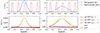 |
Fig. B.1. Top panel: The redshift distributions of the photometric sample (blue) and five out of the 20 spectroscopic samples (red) are shown. The photometric distribution on the left follows a Gaussian with parameters (μ, σ) = (0.5, 0.08), while on the right, it follows (μ, σ) = (0.5, 0.16). Bottom panel: The angular correlation is displayed for clustering only (green), magnification only (red and purple), and their sum (orange). The values of the coefficients b and α are provided in the legend. Magnification impacts the shape of the angular correlation (sum vs. clustering only) and may influence the mean redshift, particularly for larger tomographic bins (right vs. left). |
A noticeable difference is observed between clustering alone and the sum of the three effects, indicating that magnification is not entirely negligible. Since different α values are used for the spectroscopic and photometric samples, the combined effect appears to be shifted towards lower redshifts, potentially introducing a bias in the mean redshift. Finally, the impact is very limited for the narrower tomographic bin (left) but becomes more pronounced for the wider bin (right).
This highlights the importance of accounting for magnification effects when using broad tomographic bins. With UNION and LSST photometry, our bins are projected to be narrower and more localised than DES ones, and thus magnification may be negligible for Euclid clustering redshifts, even if it was not for DES.
Appendix C: Pair counts
The pair-count between two samples is theoretically given by
 (C.1)
(C.1)
where N(z) = Ntot n(z) is the number galaxy distribution. We use galaxy weights to correct selection effects, anisotropies due to observation conditions or background etc.
C.1. From continuous to discrete
In practice, the pair count is evaluated for a certain distance range rp ± Δrp. It means that for a galaxy of sample a, we are counting all the sample b galaxies within an annulus with radius rpi and width Δrpi. For instance, we use logarithmic binning, for which Δrpi ∝ rpi. Thus, the correlation (including galaxy weights) of Eq. (C.1) is related to the theoretical one through,
 (C.2)
(C.2)
C.2. Mask and estimator
There is an additional geometrical effect to Eq. (C.2) which is the mask: we do not observe the full sky. The annuli are not perfect and there is a geometrical correction
 (C.3)
(C.3)
To correct it, we compare the pair count of the correlated samples, with the ones of uncorrelated samples, submitted to the same mask, the so-called “randoms”,
 (C.4)
(C.4)
Comparing different pair counts, we always correct the amplitude, which scales as the number of objects. We usually use 10 times more randoms than objects, so we multiply DD/RR by 100. This step is done by default in Treecorr.
Computing random-galaxy pair counts, DR [which scales as 2π rpi Δrpi ηmask(rp) as well] is optimal for variance reduction (Landy & Szalay 1993). That is why our fiducial analysis involves the full Landy–Szalay estimator,
 (C.5)
(C.5)
where we omitted the galaxy number normalisation factors introduced below. A common choice for clustering-redshifts is to use the Davis and Peebles estimator
 (C.6)
(C.6)
mainly because there is no need for a random catalogue for the second sample (Davis & Peebles 1983; Gatti et al. 2018; van den Busch et al. 2020). For Euclid, a random catalogue would be created for the different analyses, so there is no motivation for using Eq. (C.6) rather than Eq. (C.5).
Appendix D: Systematic errors and bias correction
In this appendix, we provide additional tables to Sects. 4.7 and 4.8. In Table D.1, we report the values of the deviations on the mean redshift and shape due to the systematic effects. The values are the means over the five sky patches, and correspond to Δz = 0.05 and the M5 bias correction. We found similar results with other bias corrections. Finally in Table D.2, we report the values of the deviations on the mean redshift and standard deviation associated with the bias correction, in the absence of systematic effects.
Mean redshift and standard deviation bias for the different systematic effects (including none, and all) are reported; Req. refers to the requirement that needs to be fulfilled.
Mean redshift and standard deviation for the different bias corrections M0–M5, for SSM and SGP fitting, without systematics (independent case in Sect. 4.7); Req. refers to the requirement to fulfil.
Appendix E: Mis-modelling of clustering-redshifts with the one-bin approximation
In Sect. 3.2.3, we introduced an improvement to the modelling to expand beyond this one-bin approximation, which in the context of M5 bias correction is,

Since η± > 0, we expect to measure n(z) with a norm higher than unity. The global offset should be approximately
 (E.1)
(E.1)
In Fig. E.1 we show the ratio of the measured np(zi) to the true distribution, for three slicing Δz, and the five sky patches. We also report the offset predicted from Eq. (E.1) for each Δz. We observe consistency between the points and the rough prediction. Concatenating the measurements from the different redshift slices, we can express the correlation as
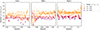 |
Fig. E.1. Deviation of the measured np(zi) to the true distribution, for different slicing Δz (points in colours), and the global offset predicted by our model, which includes correlation at the edge of the slices (solid lines in colours). The points correspond to the measurements for the five patches, hence the difference in redshift between them is not Δz. |
 (E.2)
(E.2)
where ⃗n = {n(zi)}i = 1, ..,n, Bx are diagonal matrices representing the galaxy biases, and Λ is a tridiagonal matrix, easily invertible, with unity on its diagonal and smaller terms (corrections) on the first off-diagonals. We attempted to implement Eq. (E.2) for the inference of np(z) by replacing the one-bin modelling with three-bins. We did not observe a significant improvement in the bias on the mean redshift compared to the standard renormalisation procedure, however. In Fig. E.1, we note that points from different patches at similar redshifts (visible as groups of 5 points corresponding to the 5 patches in the high-z bin) are spread over a wide range, despite the true distributions being very similar across the patches. This behaviour could be attributed to substantial sample variance, which might explain why three-bins perform similarly to one-bin. Additionally, we observe that three-bins still exhibit significant deviations in Fig. 2, highlighting the challenges of improving one-bin modelling despite our efforts. We note that in Fig. 14, the measurements for 0.75 < z < 0.85 are systematically under the true n(z) for Δz = 0.02, 0.05, which might cause the positive shift in mean redshift. This under-correlation is also visible in Fig. E.1. We did not identify its cause.
All Tables
Mean redshift and standard deviation bias for the different systematic effects (including none, and all) are reported; Req. refers to the requirement that needs to be fulfilled.
Mean redshift and standard deviation for the different bias corrections M0–M5, for SSM and SGP fitting, without systematics (independent case in Sect. 4.7); Req. refers to the requirement to fulfil.
All Figures
|
Fig. 1. Top: Simulated true-redshift distribution of each of the first ten tomographic bins (zphoto < 1.6). Bottom: Simulated redshift distribution of the spectroscopic samples from the BOSS, DESI, and Euclid surveys. The lack of spectroscopic samples for zspec > 1.8 imposes the zphoto < 1.6 condition for clustering-redshifts calibration. |
| In the text | |
|
Fig. 2. Top: Redshift distribution of sample b in blue, and four out of the ten samples ai in red. Bottom: Deviation of approximated waib with respect to the exact one for the ten cross-correlations. |
| In the text | |
|
Fig. 3. Galaxy distribution observed through different Δz averaging as Eq. (70). The redshift convolution modifies the shape of the distribution for larger slicing compared to the real slicing as estimated with a very thin slicing (grey). For this case, all slicings Δz ≤ 0.06 produce a good estimate. |
| In the text | |
|
Fig. 4. Left: n(z) distribution measurement, with 50 associated GP realisations (orange), and the true distribution (red). Middle: SNR of the GP realisation (orange), and their convolution (blue). The SNR threshold ( = 3) is reported with the dashed line. Right: Associated SGP realisations, renormalised to unity (blue), compared to the true distribution (red). |
| In the text | |
|
Fig. 5. Modelling the cross-correlation between spectroscopic samples in redshift slices and photometric bins, and reference to the corresponding tests we performed to optimise the pipeline. |
| In the text | |
|
Fig. 6. Auto-correlations of two spectroscopic samples for a single redshift bin (Δz = 0.05). The yellow and red points are obtained using the first estimator |
| In the text | |
|
Fig. 7. Variation in the Pearson coefficients rab for Flagship LRGs with ELGs. This coefficient informs on the small-scale under-correlation of blue and red galaxies. |
| In the text | |
|
Fig. 8. Pearson coefficient for our three simulated bins: low-z, mid-z, and high-z. This term is assumed to be one for clustering-redshifts calibration. We see different behaviours, r = 1, r < 1, and r > 1 for different scales and redshifts, except for the high-z bin, for which r = 1 (almost) everywhere. |
| In the text | |
|
Fig. 9. RMS of Δn, SNR of n, and reduced χ2 of Δn (top to bottom) as a function of the projected scale rp for the three redshift bins (left to right) for three bias corrections (colours). The fine lines show five independent realisations of 1000 deg2, and the thick lines show their means. |
| In the text | |
|
Fig. 10. SNR and RMS for the three tomographic bins (left to right), with three power laws as weighting functions (colours), two weighting schemes, and two bias-correction methods (M1 and M5). |
| In the text | |
|
Fig. 11. Mean redshift and shape reconstruction with SGP, for the three tomographic bins. The different markers and colours are associated with different slicing Δz. The sandy region corresponds to the Euclid requirements, and the diagonal line shows a coherent deviation of 1σ. |
| In the text | |
|
Fig. 12. Deviations on the mean-z (top) and standard deviation (bottom), with SGP fitting, for the three tomographic bins (left, middle, and right), with three Δz slicings (colours) and different implemented systematic effects (marker). The shadowed bands correspond to the Euclid requirement on both parameters. The dark and light error bars indicate 68.3% and 95.5% uncertainties |
| In the text | |
|
Fig. 13. Same as Fig. 12 for the two parameters of the SSM model, which are equivalent to ⟨z⟩−⟨z⟩true and σz/σztrue − 1. |
| In the text | |
|
Fig. 14. True-redshift distributions of tomographic bins in black, and the clustering-redshifts measurements with M5 for three spectroscopic slicings: Δz = 0.02, 0.05, 0.08 (orange, red, and purple). |
| In the text | |
|
Fig. 15. True wpp for Δz = 0.05 in grey and measurement with corrections factors including M3 as dashed green, blue, and orange lines for photo-z binning Δz = 0.1. The best fits from degree-3 polynomials are reported with solid lines. The wpp used for M3 is the best-fit model of the full correction (solid red line). |
| In the text | |
|
Fig. 16. Same as Fig. 15, but for M4, with a smaller photo-z binning Δz = 0.02. The wpp used for M4 is the best-fit model of the full correction (solid red line). |
| In the text | |
|
Fig. 17. Deviations with the SSM fitting on the mean redshift (upper panel) and standard deviation (lower panel) for the six methods M0–M5 in colour, for five sky patches (same colour). The requirements are represented by the shaded area. The dark and light error bars indicate 68.3% and 95.5% uncertainties. |
| In the text | |
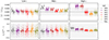 |
Fig. 18. Same as Fig. 17 with the SGP fitting. |
| In the text | |
|
Fig. 19. Uncertainties on mean-z with SSM fitting for five sky realisations in red. We also plot the best-fit uncertainty model in blue. |
| In the text | |
|
Fig. 20. True-redshift distribution of the simulated Flagship2 ten tomographic bins with zp < 1.6 (solid lines) and their clustering-redshifts measurements with our pipeline, including all systematics and realistic bias correction M3. The first two bin measurements are realised with 2500 deg2 sky patches, and the other eight are realised with 1000 deg2 sky patches. The dark and light error bars indicate 68.3% and 95.5% uncertainties, but are barely visible by eye. |
| In the text | |
|
Fig. 21. Deviations in the mean redshift (top) and the redshift standard deviation (bottom) for the ten Flagship2 tomographic bins relative to the true-redshift distributions using the SSM method. The deviations are shown for each bin and sky patch. We consider patches of 2500 deg2 for the first two bins, and 1000 deg2 for the others. The Euclid requirements on the uncertainty are highlighted by the shaded area centred around zero. The uncertainties are consistent across all the bins for the mean redshift and we achieve a clear improvement from previous work shown in red. For the redshift standard deviations, the uncertainties are slightly underestimated, but this is within an acceptable range given the requirements. |
| In the text | |
|
Fig. 22. Deviations in the mean redshift (top) and the redshift standard deviation (bottom) using the SGP method for the same bin configuration as in Fig. 21. The Euclid requirements on the uncertainty are highlighted by the shaded area centred around zero. For some bins (particularly bins 1, 3, and 7), we observe slightly larger deviations and uncertainties than permitted on the mean redshift. However, a clear improvement compared to previous work (shown in red) is still evident. The redshift standard deviations are unbiased and fall within the required range (shaded sandy area). |
| In the text | |
|
Fig. B.1. Top panel: The redshift distributions of the photometric sample (blue) and five out of the 20 spectroscopic samples (red) are shown. The photometric distribution on the left follows a Gaussian with parameters (μ, σ) = (0.5, 0.08), while on the right, it follows (μ, σ) = (0.5, 0.16). Bottom panel: The angular correlation is displayed for clustering only (green), magnification only (red and purple), and their sum (orange). The values of the coefficients b and α are provided in the legend. Magnification impacts the shape of the angular correlation (sum vs. clustering only) and may influence the mean redshift, particularly for larger tomographic bins (right vs. left). |
| In the text | |
|
Fig. E.1. Deviation of the measured np(zi) to the true distribution, for different slicing Δz (points in colours), and the global offset predicted by our model, which includes correlation at the edge of the slices (solid lines in colours). The points correspond to the measurements for the five patches, hence the difference in redshift between them is not Δz. |
| In the text | |
Current usage metrics show cumulative count of Article Views (full-text article views including HTML views, PDF and ePub downloads, according to the available data) and Abstracts Views on Vision4Press platform.
Data correspond to usage on the plateform after 2015. The current usage metrics is available 48-96 hours after online publication and is updated daily on week days.
Initial download of the metrics may take a while.