| Issue |
A&A
Volume 702, October 2025
|
|
|---|---|---|
| Article Number | A221 | |
| Number of page(s) | 13 | |
| Section | Extragalactic astronomy | |
| DOI | https://doi.org/10.1051/0004-6361/202555571 | |
| Published online | 24 October 2025 | |
Investigating the residuals in the M• – M* relation using the SIMBA cosmological simulation
1
Shanghai Astronomical Observatory, Chinese Academy of Sciences, Shanghai 200030, China
2
the University of Chinese Academy of Sciences, Beijing 100049, China
3
Departamento de Física Teórica, M-8, Universidad Autónoma de Madrid, Cantoblanco, E-28049 Madrid, Spain
4
Centro de Investigación Avanzada en Física Fundamental (CIAFF), Universidad Autónoma de Madrid, Cantoblanco, E-28049 Madrid, Spain
5
Institute for Astronomy, University of Edinburgh, Royal Observatory, Edinburgh EH9 3HJ, United Kingdom
6
Department of Physics, University of Connecticut, 196 Auditorium Road, U-3046, Storrs, CT 06269, USA
⋆ Corresponding authors: This email address is being protected from spambots. You need JavaScript enabled to view it.
, This email address is being protected from spambots. You need JavaScript enabled to view it.
Received:
19
May
2025
Accepted:
3
August
2025
Abstract
We investigate the scaling relation between black hole (BH) and stellar mass (M• − M*), diagnosing the residual Δlog(M•/M⊙) (Δ) in this relation to understand the coevolution of galaxies and BHs in the cosmological hydrodynamic simulation SIMBA. We show that SIMBA reproduces the observed M• − M* relation well, with little difference between central and satellite galaxies. By using the median value to determine the residuals, we find that the residual correlates with galaxy cold gas content, star formation rate, colour, and BH accretion properties. Both torque and Bondi models implemented in SIMBA contribute to this residual, with torque accretion playing a major role in high-redshift and low-mass galaxies, while Bondi (including BH mergers) dominates at low redshift and massive galaxies. By dividing the sample into two populations (Δ > 0 and Δ < 0), we compare their evolutionary paths by following the main progenitors. From this evolutionary tracking, we propose a simple picture for BH-galaxy coevolution: early-formed galaxies seed BHs earlier, with stellar mass increasing rapidly to reach the point of triggering ‘jet mode’ feedback. This process reduces the cold gas content and halts the growth of M*, effectively quenching galaxies. Meanwhile, during the initial phase of torque accretion growth, the BH mass is comparable between galaxies formed early and those formed later. However, galaxies that formed earlier appear to attain a marginally greater BH mass when transitioning to Bondi accretion, aligning with the galaxy transition time. As the early-formed galaxies reach this point earlier – leaving a longer period for Bondi accretion and mergers – their residuals become positive, i.e. having more massive BHs at z = 0 compared to these late-formed galaxies at the same M*. This picture is further supported by the strong positive correlation between the residuals and the galaxy age, which we propose as a validation with observation data of the scenario suggested by SIMBA.
Key words: galaxies: evolution / galaxies: formation / galaxies: general / galaxies: nuclei
Talento-CM fellow.
© The Authors 2025
 Open Access article, published by EDP Sciences, under the terms of the Creative Commons Attribution License (https://creativecommons.org/licenses/by/4.0), which permits unrestricted use, distribution, and reproduction in any medium, provided the original work is properly cited.
This article is published in open access under the Subscribe to Open model. This email address is being protected from spambots. You need JavaScript enabled to view it. to support open access publication.
1. Introduction
Galaxies of any substantial size are believed to host a central black hole (BH), with its mass, M•, scaling with the galaxy stellar mass, M*, even in dwarf galaxies (e.g. Mezcua et al. 2018a; Reines et al. 2020; Birchall et al. 2020), and at extremely high redshift (e.g. Larson et al. 2023; Kocevski et al. 2023). The initial states of these BHs, such as the ‘seeding’ mass and mass growth from the earliest phases to the massive BH stage, are still unknown (e.g. Wise et al. 2019; Haemmerlé et al. 2020; Volonteri et al. 2021, and references therein). Recent studies reveal that at high redshifts (z > 7), BH masses already exceed 108 M⊙ (e.g. Bañados et al. 2018; Wang et al. 2021a), which requires super-Eddington accretion (e.g. Alexander & Natarajan 2014). Along with their mass growth through gas accretion, BHs release large amounts of energy to galaxies through active galactic nucleus (AGN) feedback, which is observed across a broad range of redshifts (e.g. Bongiorno et al. 2014; Reines & Volonteri 2015; Mezcua et al. 2018b; Yang et al. 2023; Maiolino et al. 2024a). Such a large amount of energy is critical in hydrodynamical simulations and semi-analytic models to regulate star formation (see Heckman & Best 2014, and references therein and after) and to reproduce the observed galaxy properties (e.g. Di Matteo et al. 2005; McCarthy et al. 2011; Beckmann et al. 2017; Donnari et al. 2021; Cui et al. 2021). Whether this energy is responsible for galaxy quenching remains a topic of debate in observations; we therefore refer interested readers to detailed studies such as Aird et al. (2012), Page et al. (2012), Bongiorno et al. (2016), Bluck et al. (2020).
It has long been recognised that the growth of BHs and their host galaxies is correlated, as seen in their properties. Many observational studies report a tight correlation between the BH mass, M•, and the stellar mass, M* (e.g. Magorrian et al. 1998; Reines & Volonteri 2015; Mountrichas 2023), bulge luminosity, Lbulge (e.g. Kormendy & Richstone 1995; Kim et al. 2008; Gültekin et al. 2009; Sani et al. 2011), bulge mass, Mbulge (e.g. McLure & Dunlop 2002; Häring & Rix 2004; Kormendy & Ho 2013), and stellar velocity dispersion, σ (e.g. Merritt & Ferrarese 2001; Graham 2008; McConnell & Ma 2013; Molina et al. 2024). These scaling relations suggest the coevolution of BHs and their host galaxies, although there is considerable scatter around the median relations. This scatter, more specifically the residuals in these relations, indicates the intrinsic differences between the BHs at the same galaxy mass. Therefore, to understand the origin of this residual, it is crucial to explore how BHs form and evolve and how they interact with their host galaxies. Through this investigation, we probe the role of BHs in their coevolution with their host galaxies.
In recent decades, observational research on the M• − M* relation has primarily focused on relatively low redshifts (e.g. Cisternas et al. 2011; Sun et al. 2015; Ding et al. 2020). However, some clues about BH-galaxy coevolution remain evident through scaling relations. For example, Zhuang & Ho (2023) measure ∼11 500 broad-line AGNs at z ≤ 0.35 and find that galaxies tend to evolve towards the local M• − M* relation; i.e. when objects lie above the relation, they experience a significant increase in M*, resulting in more horizontal evolution. In contrast, objects below the relation exhibit a more pronounced growth in M•, evolving vertically, while those aligned with the relation tend to progress along it. Nevertheless, studies of faint objects and at high redshift remain scarce. This situation improved dramatically following the launch of the James Webb Space Telescope (JWST). Several studies based on the JWST have investigated the M• − M* relation at early cosmic times (z > 4) (e.g. Kocevski et al. 2023; Harikane et al. 2023; Maiolino et al. 2024b; Stone et al. 2024). Some of these studies show that galaxies at high redshift tend to host overmassive BHs compared to the local M• − M* relation (e.g. Übler et al. 2023; Harikane et al. 2023; Pacucci et al. 2023; Kokorev et al. 2023), although this difference may be enhanced by mass uncertainties and selection effects (Li et al. 2025).
Nevertheless, scaling relations at a given redshift are cumulative results over time, which makes it difficult to probe the coevolution of galaxy formation and their hosted central BHs. Comparisons between different redshifts, used to study coevolution, are also problematic because they do not directly track the progenitors. Over the last decade, this has been studied numerically by implementing empirical models into cosmological simulations and semi-analytic models (e.g. Wang et al. 2015; Nelson et al. 2015; Crain et al. 2015; Schaye et al. 2015; Dubois et al. 2016; Weinberger et al. 2017; Bower et al. 2017; Pillepich et al. 2018; McAlpine et al. 2018; Davé et al. 2019; Blank et al. 2019). However, in simulations, different BH and galaxy formation models lead to variations in their predictions of the M• − M* relation at z = 0. From the standpoint of BH mass growth, several processes are expected to affect this relation:
1.1. BH seeding mass.
To include BH particles, many simulations (e.g. Vogelsberger et al. 2014; Schaye et al. 2015; Davé et al. 2019) initialise BHs as intermediate mass (Greene et al. 2020) in the range of M• ∼ 103 − 105 M⊙, depending on conditions such as halo or galaxy mass. Therefore, different BH seeding models noticeably influence the low-mass end of the M• − M* relation and also have a substantial impact across all mass ranges at high redshift (e.g. Wang et al. 2019; Hu et al. 2022; Bhowmick et al. 2025).
1.2. BH accretion and mergers.
In simulations, BH mass mainly increases through accretion and mergers, which also play an important role in regulating the M• − M* relation (Zhu & Springel 2025). For the former, most simulations, such as TNG and EAGLE, adopt the commonly used Bondi accretion. While SIMBA additionally includes the torque model, which can bring different BH growth trajectories (e.g. Habouzit et al. 2021, 2022). Although the contribution of BH mergers to the final mass remains unclear, upcoming gravitational wave observations will allow us to quantify it more accurately.
1.3. AGN feedback.
AGNs Feedback, which releases significant amounts of energy into galactic, halo, and extragalactic environments, primarily affects the galaxy stellar mass in the M• − M* relation by regulating galaxy cold gas content and star formation activities (e.g. Ma et al. 2022; Liu et al. 2025), especially at the high-mass end (e.g. Li et al. 2020; Habouzit et al. 2021). As the key connection between the BH and its host galaxy, AGN feedback plays an important role in their coevolution.
To shed light on BH-galaxy coevolution, we propose using BH mass residuals, i.e. the relative BH mass difference at a given galaxy stellar mass, which provide a unique perspective. In this work, we use the SIMBA simulation (Davé et al. 2019) to explore the origin of the residual in the M• − M* scaling relation and its implications for BH-galaxy coevolution. We correlate the residual with galaxy and BH properties and investigate how BH accretion and cold gas evolution influence the residual and the growth path of M• − M*.
This paper is organised as follows: In Section 2, we present basic information about the SIMBA simulation and describe its BH accretion and feedback models. In Section 3, we show the residual of the M• − M* scaling relation and its correlation with galaxy and BH properties. In Section 4, we investigate the origin of the residual and BH-galaxy coevolution. Section 5 provides a discussion, and we summarise our main findings in Section 6.
2. The SIMBA simulation
The SIMBA simulation (Davé et al. 2019) is a cosmological hydrodynamic simulation based on MUFASA (Davé et al. 2016), running in the meshless-finite-mass mode of the GIZMO code (Hopkins 2015). We focus on the simulation run m100n1024, which has a box size of 100 h−1 Mpc on the side, containing 10243 gas particles and 10243 dark matter particles. The mass resolution is 9.6 × 10⁷ M⊙ for dark matter and 1.82 × 10⁷ M⊙ for gas particles. The adopted cosmology is based on Planck Collaboration XIII (2016) with parameters: ΩM = 0.3, ΩΛ = 0.7, Ωb = 0.048, and H0 = 68 km s−1 Mpc−1.
In SIMBA, galaxies are identified using a 6D friends-of-friends (FoF) algorithm with a linking length of 0.0056 times the mean particle separation. The Galaxy properties, such as stellar mass, M*, star formation rate (SFR), and metallicity, are characterised by the CAESAR analysis package1. Star formation is directly modelled following the relation of Schmidt (1959), by calculating the molecular gas fraction of the total gas, fH2, following the subgrid prescription of Krumholz & Gnedin (2011). The SFR is calculated as  , where ϵ* = 0.02 (Kennicutt 1998), ρ is the gas density, and tdyn is the local dynamical time. Star formation occurs when
  . The H I fraction is calculated based on the prescription of Rahmati et al. (2013), which accounts for the self-shielding effect. The H I and H2 are computed on the fly self-consistently in SIMBA, with their combined amount representing the total neutral gas.
SIMBA adopts the on-the-fly FoF algorithm to seed BHs in galaxies. BHs are placed in galaxies when M* > γBH × Mseed, with Mseed = 104 M⊙/h and γBH = 3 × 10⁵. After seeding, BHs grow through a two-mode accretion model. Torque accretion (Anglés-Alcázar et al. 2015, 2017) is for cold (T < 105K) gas within the BH kernel, with gas inflow rate ṀTorque driven by disc gravitational instabilities (Hopkins & Quataert 2011). Bondi accretion (Bondi 1952) is for hot (T > 105 K) non-ISM gas, with the gas inflow rate referred to as ṀBondi. The total accretion rate is calculated as Ṁ∙ = (1−η) × (ṀTorque + ṀBondi, where the radiative efficiency η is set to 0.1.
The BH feedback in SIMBA consists of kinetic feedback and X-ray feedback. The kinetic feedback model is motivated by two-mode AGN feedback in observations: the ‘radiative mode’ at high accretion rate, and ‘jet mode’ at low accretion rate. These are divided by the Eddington ratio,  , where Medd is the Eddington accretion rate:
  . The radiative mode mimics the radiative AGN winds; the outflow velocity is based on M• and is typically around 1000 km s−1. The jet mode arises when fedd < 0.2 and
  . The outflow velocity increases strongly as fedd drops and reaches the full speed ∼8000 km s−1 when fedd ≤ 0.02. When the full-velocity jet is triggered and the gas fraction is fgas = Mgas/M* < 0.2, X-ray feedback is included to heat the surrounding gas. We refer the reader to Davé et al. (2019) for more details. In this study, we restricted the analysis to galaxies with stellar mass
  and BH mass M• > 5.0 × 10⁶ M⊙ at all redshifts, to ensure that only well-resolved galaxies and BHs are included.
3. Black hole – galaxy scaling relations
The connection between the mass a galaxy and its central supermassive BH has been shown to be linearly correlated over orders of magnitude in logarithmic space, in the form
 (1)
(1)
Thanks to the torque accretion model (Anglés-Alcázar et al. 2013, 2015, 2017), the SIMBA simulation is able to reproduce this scaling relation, as presented in Davé et al. (2019), along with other BH and AGN statistics (Thomas et al. 2019). In Figure 1, we revisit this relation by separating central galaxies from satellite galaxies and fitting the M• − M* relation using the median values of M• in each M* bin. The median values and corresponding fits for both central and satellite galaxies agree well with the observational line from the M• − Mbulge relation in Kormendy & Ho (2013) (KH2013). Although the best fit for satellite galaxies tends to deviate from that of centrals and from observations at low M* (with slightly higher M•), the median data points are well aligned. A plausible explanation is that satellite galaxies in massive haloes tend to be stripped to lower M* compared to centrals. Because this difference is minimal, we do not separate central and satellite galaxies in this study unless noted.
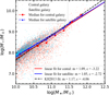 |
Fig. 1. Scaling relation between M• and M* for central and satellite galaxies, shown as red and cyan dots, respectively. The best-fit power-law relations for central (red line) and satellite galaxies (blue line) are compared to the observational results from Kormendy & Ho (2013) (KH2013, dashed black line), and the best-fit parameters are given in the lower-right legend. The plot highlights the very small discrepancy between central and satellite galaxies and the observed relation. |
In Figure 2, we show the M• − M* relation for galaxies at z = 0, z = 1, z = 2 and z = 3, from left to right, colour-coded by  . At a given stellar mass, galaxies tend to have higher BH masses as SFR decreases. Quiescent galaxies host more massive BHs and show a smoother decline in SFR with M• at z ≤ 2, a trend also seen in Illustris, IllustisTNG, and EAGLE (Terrazas et al. 2016, 2020). We fit the median log M• in each log M* bin (black crosses). The best-fit results are shown as solid black lines, with the linear fitting parameters given in the bottom legend. Instead of using the original fit to all the data (e.g. Shankar et al. 2025), we used the median points to avoid the fitting line tilting lower at low galaxy stellar mass due to the large spread of data points in that region. Our results show a mild evolution from z = 3 to z = 0. At a given stellar mass bin, more massive BHs are found at lower redshift. The SFRs of massive galaxies above the scaling relation begin to decrease earlier than those below it, and galaxies quench when M• > 108 M⊙. This is caused by the jet mode AGN feedback in SIMBA, as discussed in the following sections.
 |
Fig. 2. Scaling relation between M• − M* for galaxies at z = 0, z = 1, z = 2, and z = 3, shown from left to right, colour-coded by log SFR. The median M• value in each M* bin is shown as black dots. The black lines represent the best-fit relation to these median values and are used as the median M• − M* scaling relation when calculating residuals. The best-fit parameters are presented in the legend at the bottom. Galaxies with lower SFR at a given M* tend to host more massive BHs. |
As shown in Habouzit et al. (2021), SIMBA agrees with TNG simulations and shows the relation evolving from a lower normalisation to higher values at z = 0. In contrast, Illustris, Horizon-AGN, and EAGLE show the opposite redshift evolution, i.e. a higher M• − M* normalisation at higher redshift. In the BRAHMA simulation, Bhowmick et al. (2025) explores five different BH seeding models, finding that the seeding models noticeably affect the M• − M* relation, particularly at the low-mass end, and substantially impact all mass ranges at high redshift. Although recent discoveries of supermassive BHs at very high redshift tend to favour a decreasing evolution (see, Ding et al. 2020, for example), as suggested by Illustris, Horizon-AGN, EAGLE, and UniverseMachine (Terrazas et al. 2024), larger samples and more consistent studies are needed to reach a firm conclusion.
As indicated by the colour bar in Figure 2, there is a meaningful scatter around the median M• − M* relation. To better quantify this, we defined the residual Δlog(M•/M⊙) (Δ) in the M• − M* scaling relation as the difference between the actual galaxy log(M•/M⊙) values and their corresponding best-fit log(M•/M⊙) values at the given stellar mass log(M*/M⊙), i.e.
 (2)
(2)
We explore the correlation between the residual and galaxy and BH properties in Section 3.1 and Section 3.2.
3.1. Relation between residuals and galaxy properties
Figure 3 shows the correlations between the residuals and various galaxy properties. Panels from top to bottom display galaxy SFR, H I mass ( ), H2 mass (MH2), and metallicity (Z). From left to right, the panels show these relations at z = 0, z = 1, z = 2, and z = 3. Data points are colour-coded by log M*. Correlation coefficients are shown at the bottom of each panel. For all correlations, we used the Pearson correlation coefficient, which is based on the proportion of covariance to the standard deviation of the initial data. These coefficients are provided to roughly indicate their relevance and are mainly used to compare different redshifts. We also examined other galaxy properties, but only those with high correlation coefficient values are shown in Figure 3. For example, although the SFR is closely related to galaxy colour2, the correlation between galaxy colour and the residual is much weaker, as shown in Figure 4 at z = 0. The correlations between residuals and galaxy colour become even weaker at higher redshift.
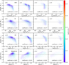 |
Fig. 3. Correlations between residuals and galaxy properties. Panels from top to bottom show galaxy SFR, H I mass ( |

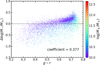 |
Fig. 4. Correlation between residual and galaxy colour g − r at z = 0, colour-coded by log M*. The correlation coefficient between colour and the residual is shown at the bottom. |
The SFR shows a strong negative correlation with the residual, consistent with Figure 2. In addition, galaxies with higher BH mass (larger Δlog M• ) tend to have smaller cold gas reservoirs (both H I and H2), but higher metallicity and redder colour at z = 0 (see also Cui et al. 2024). This indicates that star formation activity and cold gas content play a significant role in regulating the M• − M* relation. Phenomenally, large cold gas reservoirs fuel star formation, keeping galaxies blue and enabling them to have larger M* with lower residuals, i.e. lying below the relation. When cold gas is consumed, expelled, or heated, galaxies begin to quench: the growth of M* slows, galaxies tend to redden and have less cold gas and higher metallicity. This leads to increased and larger residuals, i.e. lying above the relation. Here we focus only on the effect of galaxy stellar masses on the residual, without considering variations in BH mass, which will be examined in the following section.
3.2. The relation between the residual and BH accretion
Similar to Figure 3, Figure 5 shows the correlation between the residual and BH accretion properties at z = 0, z = 1, z = 2, and z = 3. Panels from top to bottom show the BH mass attributed to torque accretion (MTorque), the torque accretion rate (ṀTorque), the BH mass attributed to Bondi accretion (MBondi), the Bondi accretion rate (ṀBondi), and the Eddington ratio (fedd), colour-coded by log M*. We show the BH accretion rate ∼0 as 10−7 at each redshift.
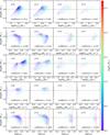 |
Fig. 5. Correlations between the residual and BH properties. Panels from top to bottom show BH mass attributed to torque accretion (MTorque), the torque accretion rate (ṀTorque), BH mass attributed to Bondi accretion (MBondi), the Bondi accretion rate (ṀBondi) and the Eddington ratio (fedd), colour-coded by log M*. Red dashed lines in the bottom row indicate fedd = 0.2, where jet mode feedback is triggered. In the panels for ṀTorque, ṀBondi, and fedd, BHs with zero accretion rate are assigned a value of 10−7. Panels from left to right show these relations at z = 0, z = 1, z = 2, and z = 3, respectively. Correlation coefficients between these relations are shown at the bottom of each panel. |
As expected, MTorque and MBondi correlate positively with the residual. As discussed in Section 2, torque accretion primarily drives BH growth by accreting cold gas near the BH, whereas Bondi accretion facilitates growth through the accretion of hot gas. The increasing masses associated with these accretion modes lead to the growth of BH mass and a larger residual. Residuals of galaxies with similar M* follow the same linear correlation with MTorque, unlike the relation with MBondi. This indicates that torque accretion does not significantly impede the growth of M*, suggesting that the growth of the BH and M* are synchronised during this phase. Therefore, we expect that Bondi accretion plays a more important role in increasing this scatter in SIMBA, as indicated by the stronger correlation coefficients of residuals with MBondi compared to MTorque, especially at lower redshift. However, the relation between MBondi and the residual truncates at log(MBondi/M⊙)∼5. This truncation occurs when log(M•/M⊙)∼8, where jet-mode feedback begins. This indicates that when BHs grow larger, jet-mode feedback plays a crucial role in heating cold gas, substantially enhancing the Bondi accretion rate and quenching galaxies by increasing the amount of hot gas, thereby modulating the growth of the BH and its host galaxy.
Overall, ṀTorque exhibits a negative correlation with the residual, whereas ṀBondi correlates positively. However, at z > 0, for BHs with residuals smaller than 0 (Δ < 0), ṀTorque positively correlates with the residual. In these cases, ṀTorque is relatively high, and only a small fraction of BHs have initiated Bondi accretion, so BH growth is primarily driven by torque accretion. In contrast, for BHs with residuals Δ > 0, ṀTorque is negatively correlated with the residual. In these systems, the BH has grown above the M• − M* scaling relation and Bondi accretion increases, leading to rapid BH growth as torque accretion diminishes. A positive correlation is observed between ṀBondi, the residual, and stellar mass for BHs with Δ > 0, suggesting that once Bondi accretion becomes strong, it significantly enhances the mass growth of all BHs.
The Eddington ratio, fedd, is defined as Ṁ∙/Ṁedd, where Ṁedd is proportional to the BH mass. In terms of Ṁ∙, more than 80% of BHs have fedd dominated by ṀTorque, which is also the dominant component of Ṁ∙ as seen in Figure 5. Although ṀBondi is positively correlated with the residual, fewer than 40% of BHs have ṀBondi > 0 at each redshift, and only ∼10% at z = 3. These BHs with ṀBondi > 0 are mostly hosted by the most massive galaxies at z = 0. Residuals therefore anti-correlate with fedd, similar to ṀTorque. If we naively take fedd as Ṁ∙, the negative correlation of residuals with fedd and the galaxy SFR will imply a positive correlation between Ṁ∙ and galaxy SFR, consistent with previous studies (e.g. Chen et al. 2013; Aird et al. 2019). In Figure 5, vertical red dashed lines mark fedd = 0.2, which denote the starting point of jet-mode feedback in SIMBA. Interestingly, most (∼95%) BHs enter jet-mode feedback (fedd < 0.2 and  ) after z ∼ 1, but these systems remain dominated by torque accretion, which naturally produces declining median Eddington ratios at lower redshift (Anglés-Alcázar et al. 2015). More massive BHs tend to have lower fedd. On the one hand, this potentially increases the BH mass, especially in low-mass galaxies, as suggested by Manzano-King et al. (2019), because AGN outflow is an important and potentially dominant source of feedback in low-mass galaxies, capable of suppressing stellar mass growth and thereby elevating M•. On the other hand, this does not seem to agree with AGN activity in dwarf galaxies found in observations. For example, Mezcua & Domínguez Sánchez (2024) found only ∼20 per cent of dwarf galaxies in MaNGA host AGN activity.
3.3. Indication of the M• − M* scaling relation
From Figures 2 to 5, we see that in SIMBA, the residuals correlate with both galaxy and BH properties. This is a meaningful and interesting quantity for interpreting and investigating the M• − M* relation and its evolution. Properties such as the cold gas content and BH growth may be responsible for the residuals in the M• − M* relation. From these figures, we hypothesise that galaxies have a large amount of cold gas at high redshift, fuelling star formation to grow stellar mass and maintain galaxies blue, while also providing the torque accretion required for rapid BH growth. Galaxies below the scaling relation are expected to have slightly more cold gas and lower metallicity. When BHs reach ∼108 M⊙, jet-mode AGN feedback activates. Bipolar jets eject gas particles surrounding the central BH vertically at high velocity. These gas particles will become wind particles, which first decouple from the hydrodynamic calculation in the simulation to travel almost freely for 0.0001 Hubble time (Davé et al. 2019). It then becomes a normal gas particle, entering the hydrodynamic calculations and heating up their surrounding gas particles through shock heating. This significantly reduces the total cold gas within and around galaxies (Ma et al. 2022) and further promotes BH growth through Bondi accretion. Galaxies then lose cold gas and start to quench and, as a result, the residuals begin to grow.
This coevolution process is also suggested by observations. Terrazas et al. (2016) find that quiescent galaxies host more massive BHs than star-forming galaxies with similar stellar masses at z < 0.034, i.e. quiescent galaxies have a positive residual in the M• − M* relation, where AGN feedback supresses star formation. Similarly, Martín-Navarro & Mezcua (2018) points out that BHs above the mean M• − σ scaling relations tend to reside in galaxies with lower SFR. With the advantage of simulations that allow us to track galaxy and BH evolution over time, we verify that assumption in the following sections.
4. Coevolution of BHs and galaxies
4.1. BH and galaxy coevolution
To further investigate how galaxies and BHs coevolve from high redshift to z = 0 in SIMBA, we traced the growth of BHs with  and their host galaxies with
  at z = 0. Figure 6 shows the distributions of M• − M*, MTorque − M*, and MBondi − M*, from top to bottom. The most massive progenitor in the previous snapshot is defined as the main progenitor. Each data point in Figure 6 marks the position of a progenitor galaxy and its BH in the M• − M* relation. Thus, the growth path of each galaxy can be traced as a series of dots with the same colour, colour-coded by the residual at z = 0 (Δz = 0). We show the evolution for galaxies in different stellar mass ranges and with Δ. To calculate the median lines, we used median stellar and BH masses for each snapshot when there are at least 20 galaxies in each snapshot. When a galaxy lacks a BH, its BH mass was considered as zero, and these values were included in the calculation of the median.
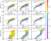 |
Fig. 6. Galaxy and BH coevolution history traced by M* and BH masses. Panels from top to bottom show the M• − M*, MTorque − M* and MBondi − M* relations as data points colour-coded by their residuals at z = 0 (Δz = 0). Columns from left to right show galaxies with stellar mass at z = 0 in the ranges 10.0 < log(M*/M⊙) < 10.5, 10.5 < log(M*/M⊙) < 11, and 11.0 < log(M*/M⊙) < 13. The galaxy number (n) in each stellar mass bin at z = 0 is given in the top-left corner. For reference, we show the scaling relation at z = 0 from Figure 2 as a black solid line. Median growth histories for galaxies with Δ > 0 and Δ < 0 are shown as red and blue solid lines, respectively, with the start redshifts of growth labelled. The separation time ZΔ, sep of M• − M* growth histories for the Δ > 0 and Δ < 0 populations, defined as the epoch when variance between their median growth trajectories first exceeds 0.1 dex, is indicated by large black dots. The separation time ZTorque, sep between the median M• − M* and MTorque − M* is marked with filled stars: red for Δ > 0 and blue for Δ < 0. To highlight these differences, the redshifts of ZΔ, sep and ZTorque, separe labelled in the first row, in red for Δ > 0 and blue for Δ < 0. |
To identify when the M• − M* growth histories of Δ > 0 and Δ < 0 populations diverge, we defined a separation time ZΔ, sep, at which the variance between their BH masses of median growth trajectories exceeds 0.1 dex for the last time. We likewise defined the separation time ZTorque, sep, when the differences between the median growth trajectories of M• − M* and MTorque − M* exceed 0.05 dex, which is marked as filled stars. These stars mark when the total BH mass growth is no longer dominated by the torque mass.
Figure 6 does not explicitly show redshift information, that is, data points at the same position can correspond to galaxies at different redshifts. To highlight this, we include several redshifts in the plot (red for Δ > 0 and blue for Δ < 0), with the redshifts at the bottom indicating the median starting redshift of each median line. Galaxies with Δ > 0 have higher starting redshifts than those with Δ < 0 in all three stellar-mass bins. The quantity ZΔ, sep is shown in the middle of the plots in the top row, which agrees with the starting redshift difference. This indicates that the torque model is affected by the galaxy growth history, driving the first deviations in the M• − M* relation. The ZTorque, sep values are shown at the top of the first-row panels, which highlights the influences of the Bondi module on the residuals. Bondi accretion contributes much later but drives the deviations to a larger value. This plot also explains why the M• − M* relation at high redshift lies lower than at low redshift: the initial growth of BH falls below the relation at z = 0. From the perspective of the galaxy, stellar mass growth is much more efficient at high-z compared with low-z, because star formation and the amount of cold gas systematically decrease over time due to AGN feedback3. As a result, low-z galaxies are more affected by the growth of M*, and the M• − M* relation is higher at low redshift.
In all stellar-mass bins, the growth of the M• − M* relation for galaxies with either Δ > 0 or Δ < 0 almost overlaps before ZΔ, sep. Almost all data points lie in the same region without clear separation until a very late redshift. The subtle difference can only be seen through the median lines. Galaxies with Δ > 0 then have higher BH masses than those with Δ < 0. Before ZTorque, sep, the M• − M* relation closely follows the MTorque − M* growth trajectory for all galaxies. After ZTorque, sep, i.e. when z ∼ 0 and log(M•/M⊙)∼8, jet-mode AGN feedback is triggered. It expels cold gas from galaxies and heats the cold gas within them. This process rapidly promotes Bondi accretion, which applies to hot gas. The significant growth of MBondi drives the rapid growth of M•. Simultaneously, torque accretion slows, causing the separation of M• − M* and MTorque − M*. As a consequence, the M• − M* growth trajectory moves vertically towards the scaling relation at z = 0 for galaxies with log(M*/M⊙) > 10.5. Galaxies that begin Bondi accretion earlier move above the scaling relation at z = 0 and become quenched. For galaxies with log(M*/M⊙) > 11 and Δ > 0, the growth of MBondi slows as redshift approaches zero. The growth of these massive galaxies is also influenced by mergers, which further contribute to the increase in BH and stellar masses (e.g. Hirschmann et al. 2015; Habouzit et al. 2021).
4.2. Physical drivers of the residual
Figure 6 shows the general M• − M* evolution trend: BHs and galaxies simultaneously increase towards the relation at z = 0, particularly at high redshift. The plot highlights the information on the initial state, which depends on the simulation resolution and the BH seeding mass. At lower redshifts, it is unclear when BH and galaxy stellar masses stabilise, i.e. no clear evolution results in the intermediate phase of growth trajectory in Figure 6. Furthermore, distinct mass-assembly phases driven by accretion mechanisms and feedback processes are inferred only by several hypotheses. This raises the question of what factors lead to the different mass assembly phases and how these individual evolutions can be quantitatively characterised. More importantly, whether the same mass growth of BHs and galaxies drives the similarity in the M• − M* relations between different redshifts remains an open question. In the following, we investigate in more detail how BHs accumulate mass via accretion processes and mergers, and how galaxies grow through star formation and the evolution of their cold gas reservoirs over time.
Figure 7, presents the growth history of BHs and galaxies in different stellar-mass ranges and Δ. The top row shows the median evolution of M•, and the mass fractions of torque accretion (fTorque = MTorque/M•), Bondi accretion (fBondi = MBondi/M•), and BH mergers (fMerge = MMerge/M•). The bottom row shows the evolution of M*,  , MH2, and SFR. We also marked ZΔ, sep and ZTorque, sep in the panels.
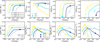 |
Fig. 7. Median growth histories for different galaxy quantities. The top row shows the evolution of M•, fTorque, fBondi, and fMerge with time from left to right. The bottom row shows the evolution of M*, |

Figure 7 shows that BHs with Δ > 0 begin their growth earlier than those with Δ < 0. This also applies to their host galaxies, owing to the seeding scheme in SIMBA in which BHs are seeded based on the host galaxy mass. Consequently, earlier-forming galaxies will have BH seeded earlier. For BHs in galaxies with log(M*/M⊙) < 11, torque accretion (fTorque) dominates the growth of BH mass, contributing a larger fraction than Bondi accretion (fBondi) or mergers (fMerge). Specifically, BHs in galaxies with 10 < log(M*/M⊙) < 10.5 and Δ < 0 rely almost entirely on torque accretion. With time, the relative contribution of torque accretion diminishes, while Bondi accretion and mergers become increasingly significant. In the most massive systems (11 < log(M*/M⊙) < 13), Bondi accretion and mergers surpass the contribution from torque accretion and dominate BH growth at z = 0. For BHs with Δ > 0, merger contribution tends to become more significant slightly later than Bondi accretion.
On the galaxy side (Figure 7, bottom panels), stellar mass growth is primarily driven by star formation from cold gas reservoirs (MH I and MH2). In the early Universe, rapid M* growth is due to the large amount of cold gas and high SFRs. In Figure 6, galaxies with Δ > 0 and Δ < 0 share similar M• − M* growth trajectories before ZΔ, sep, which corresponds to the epoch when MH I peaks (the second panel in the bottom row of Figure 7). Subsequently, in galaxies with log(M*/M⊙) < 11, those with Δ > 0 experience a faster decline in MH I after reaching the peak, slowing torque accretion and the growth of M* earlier compared to those with Δ < 0. For the most massive galaxies (11 < log(M*/M⊙) < 13), the differences between Δ > 0 and Δ < 0 become smaller: they exhibit similar MH I, undergo substantial mergers, and their M• − M* growth histories show little variation, consistent with what is shown in Figure 6. H I is located on the outskirts of galaxies, acting as the supply of H2 and revealing the total cold gas reservoir of galaxies (e.g. Wong & Blitz 2002; Kennicutt et al. 2007; Bigiel et al. 2008). As SIMBA uses an H2-based star formation model, SFR evolution closely follows H2 mass evolution (bottom-right panel). The longer and higher SFR in these Δ < 0 galaxies yield higher stellar masses at z = 0, and their BHs remain less massive than those galaxies of the same M* with Δ > 0. We also find that galaxies with Δ > 0 occupy denser environments than those with Δ < 0 after ZΔ, sep, which would deplete their H I more quickly. For the underlying physical mechanism behind this rapid H I depletion, we propose two main causes: (1) environmental effects such as ram pressure stripping or tidal events (e.g. Brown et al. 2017; Cortese et al. 2021; Wang et al. 2021b, 2022), or (2) earlier, and thus longer AGN feedback heating the gas and reducing the H I mass (discussed further below).
Before ZTorque, sep, H2, and SFR increase continuously, ensuring that torque accretion remains dominant and that growth of M• − M* and MTorque − M* remains consistent, as shown in Figure 6. When cold gas reservoirs and SFRs peak, that is, after ZTorque, sep, BH masses have already reached 108 M⊙. At this point, jet mode feedback is triggered, ejecting cold gas and increasing the density of hot gas within subhaloes. The reduced cold gas suppresses torque accretion and star formation, gradually quenching galaxies. Meanwhile, BH growth begins to increase by Bondi accretion. At this stage, the growth trajectories of M• − M* and MTorque − M* diverge (as indicated by star symbols in Figure 6). In galaxies with Δ > 0, BHs experience more significant and earlier Bondi accretion, along with more mergers, leading to overmassive BHs. In the most massive galaxies, BH mergers contribute comparably to Bondi accretion at z = 0. Both contributions decrease with galaxy stellar mass, with the BH mass in low-mass galaxies still dominated by torque accretion. Meanwhile, galaxies that host undermassive BHs (Δ < 0) experience a longer period of star formation, which declines slowly, delaying the cessation of M* growth to a later stage compared to galaxies with overmassive BHs. This behaviour occurs despite galaxies have similar SFRs in the early Universe, which has also been reported in Martín-Navarro et al. (2018) and suggested in Cui et al. (2021).
Most galaxies with Δ > 0 begin their growth earlier than those with Δ < 0, as indicated by the redshifts at the bottom of each panel in Figure 6. This provides Δ > 0 galaxies with more time to form stars and accumulate torque and Bondi accretion, allowing their BHs to grow more significantly than in the Δ < 0 population and therefore produces a larger residual. The different residuals of galaxies are partially attributed to differences in the times of galaxy formation. To quantify the relation between growth time and residual, we fit the galaxy formation history as an error function and defined the transition time (ZG, tran) for each galaxy following Eq. 1 of Cui et al. (2021). This is the redshift when the growth slope is less than 0.1, i.e.
 (3)
(3)
Unsurprisingly, this ZG, tran aligns with ZTorque, sep (Figure 7). We also consider the observable mass-weighted galaxy age, which is closely connected to the galaxy transition time. For consistency, the galaxy mass-weighted age is converted to the redshift through the Universe’s look-back time. With this quantity, which can be measured observationally, the SIMBA model of M• − M* coevolution can be verified against observational results.
Figure 8 shows the correlations between the residuals Δ and the redshift when BHs seeded (ZBH, seed), galaxy transition time (ZG, tran), and galaxy age (for uniformity, we converted the galaxy age to the redshift when they formed, ZG, form). The same three galaxy stellar mass bins (10.0 < log(M*/M⊙) < 10.5, 10.5 < log(M*/M⊙) < 11, and 11.0 < log(M*/M⊙) < 13) are presented. To highlight the significance, we also include the correlation coefficient between Δ and these quantities for each mass bin. The positive correlations between Δ and the three quantities confirm our earlier claims regarding why some galaxies host low-mass BHs while others can nurture massive BHs.
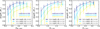 |
Fig. 8. Relation between residuals and the redshifts of BH seeding (ZBH, seed, left panel), galaxy transition (ZG, tran, middle panel), and galaxy formation (ZG, form, right panel). Galaxies with stellar mass ranges 10.0 < log(M*/M⊙) < 10.5, 10.5 < log(M*/M⊙) < 11, and 11.0 < log(M*/M⊙) < 13 are shown as navy, cyan, and yellow lines, respectively, with errors estimated from the 16th to 84th percentile ranges. Correlation coefficients for each stellar mass bin are shown in each panel in the corresponding colours. |
However, the correlation between residuals and ZBH, seed appears saturated when ZBH, seed is high and Δ > 0.2. The correlation curve plateaus at slightly different redshifts for different mass bins, being somewhat higher for the more massive bins. This implies two things: (1) there may be a maximum BH mass of the galaxy at a given mass, which cannot be exceeded, even if it is seeded at the highest possible redshift. Because the BH mass residual is anti-correlated with the galaxy SFR, these galaxies with high ZBH, seed are formed considerably earlier and are quenched earlier. After quenching, both the galaxy stellar mass and the BH mass almost halt, as shown in the left panels of Figure 7. (2) The plateau also indicates that above a certain ZBH, seed, even early-formed galaxies will not push the BH mass even higher. This implies that the coevolution between the BH and galaxy after quenching becomes self-similar: either both the BH and the galaxy masses stop growing entirely, or they both increase along the M• − M* relation.
The effects of BH seeding mass, particularly on the scatter of the M• − M*, are presented in several studies (e.g. Habouzit et al. 2021; Zhu & Springel 2025). As noted in Habouzit et al. (2021), the BH seeding mass should affect these simulations with only the Bondi accretion model ( more than SIMBA, where the torque accretion only weakly depends on the BH mass as the form of
  (Anglés-Alcázar et al. 2013, 2015)). This is consistent with our result that the final BH mass is related to the BH seeding time, not the seeding mass. Furthermore, we show that the scatter arises from both accretion models, with the Bondi model, as well as mergers, contributing more strongly for massive galaxies at low redshift (see e.g. Zou et al. 2024).
Since BH seeding in SIMBA is based on the galaxy stellar mass, an early BH seeding time corresponds to an early-formed galaxy and, as such, a higher galaxy transition redshift. Following Cui et al. (2021), at the same stellar mass, galaxies with higher transition redshift tend to reside in late-forming haloes, i.e. smaller haloes at high redshift. This facilitates faster consumption of cold gas, transferring the BH accretion to Bondi mode. Higher BH mass at the galaxy transition time and an extended Bondi accretion period further increase the BH mass, resulting in positive residuals. The relation between Bondi accretion and BH mergers can be viewed as mutually reinforcing; for example, Bhowmick et al. (2020) suggested that merging BHs tend to have high Eddington ratios, indicating elevated BH accretion rates.
These assumptions are supported by the previous figures. However, to confirm this observationally, we need to connect these results to observable quantities. Given that early transition times lead to red galaxies (Cui et al. 2021), it is not surprising to see the positive correlation between Δ and ZG, form. This allows our theoretical predictions to be tested with observational data. As suggested by Habouzit et al. (2022), the BH mass offsets of the simulated faint quasar population at z ≥ 4 represent the offsets of the entire BH population across all simulations, which can be used to present the entire BH offsets.
5. Discussion
5.1. Scatter and residuals
In observations, the scatter in the M* − M• relation is often related to observation uncertainties, systematics, and quantity-derivation methods. Observations generally report a scatter larger than 0.5 dex, (see Graham 2012; Davis et al. 2018; Baron & Ménard 2019; Li et al. 2023, for example), while the scatter from simulations is typically smaller than 1 dex (Habouzit et al. 2021; Zhu & Springel 2025). On the one hand, simulations probe the intrinsic scatter, which is expected to be smaller than in observations; on the other hand, this could be related to the lack of stochasticity in the galaxy-BH subgrid. Zhu & Springel (2025) found that the scatter in low-mass galaxies can be significantly reduced by AGN feedback, while at the high-mass end, it is decreased by the hierarchical merging of quenched systems. This was also found by Hirschmann et al. (2010), who showed that the intrinsic scatter of the M• − Mbulge relation decreases with an increasing number of mergers and, consequently, with time. However, these scatter studies can only reflect certain systematics, making it difficult to extract useful information on the BH-galaxy relation. Unlike scatter, which only quantifies standard deviations, the residual can be directly linked to differences in BH mass growth, allowing us to ask why some BHs accrete more mass than others at the same M*
It is well known from observation that the M• − M* relation has different slopes depending on the galaxy types used for the fitting function (e.g. Davis et al. 2019; Graham & Sahu 2023, for more recent results). Shankar et al. (2025) report that the correlation between the residuals of the BH scaling relations (M• − Mbulge, M• − σ) may result from kinetic AGN feedback. However, increasing the kinetic output of AGN feedback does not improve alignment with observational data. Marasco et al. (2021) investigated the residuals in the galaxy global star formation efficiency f* − M• relation versus those in the M• − Mhalo relation, finding that galaxies in lighter haloes have larger f* at the same M•. Although this is not directly presented in our study, it qualitatively agrees when combining the findings of Cui et al. (2021), which indicated that blue galaxies generally inhabit lower-mass haloes, with the results shown in Figure 2, which demonstrate that massive galaxies are more likely to be star-forming at a fixed BH mass. In addition, combining the results from Cui et al. (2021), we expect that low-mass BHs tend to reside in low-mass haloes at the same galaxy stellar mass4. This theoretically explains why the M• − Mhalo relation is also very tight. Nevertheless, directly linking this residual to galaxy properties provides a novel insight into BH growth and how it connects with galaxy evolution. Furthermore, the BH mass residuals computed for the entire BH population are crucial to understand the build-up of BHs (Habouzit et al. 2022), which we discuss in the next subsection.
5.2. Coevolution from the perspective of residuals
Li et al. (2024) separate BH growth in the TNG simulation into four distinct phases. Their Figure 2 shows minimal differences in the cumulative distributions between phase one (star formation, BH seed dominates) and phase two (rapid SMBH growth), as well as between phase three (self-regulation and galaxy quenching) and phase four (mergers). A similar feature can also be found in SIMBA, but for simplicity, we merged the two initial phases as the torque growth stage and the last phases into a Bondi and merger stage, following the approach of Mo et al. (2024) (see also Boco et al. 2023). The first stage is dominated by torque accretion. Early in galaxy formation, the amount of cold gas rapidly increases, which can supply star formation and rapid BH growth via torque accretion. During this phase, earlier-forming galaxies have more cold gas in the early Universe, growing M* and M• faster, leading to higher stellar and BH masses relative to those galaxies formed later after ZΔ, sep. The second stage begins at ZTorque, sep. Once the BH mass increases to ∼108 M⊙, jet-mode feedback starts, rapidly depleting and heating the cold gas. The BH growth supplied by torque accretion slows and begins to be dominated by Bondi accretion. The growth trajectories of M• − M* and MTorque − M* separate, H I is consumed, and both H2 and SFR begin to decrease. Galaxies experience a deceleration in M* growth and initiate quenching. Black holes seeded later result in a slower decline of cold gas and SFR, allowing for a longer period of star formation and a smaller fraction of Bondi accretion, maintaining Δ < 0. Furthermore, the evolution of neutral hydrogen gas mass (including both H2 and H I) with SFR in massive central disk galaxies is suggested as a critical constraint of BH feedback models across several simulations (Shi et al. 2022).
6. Conclusions
This work uses the SIMBA simulation (Davé et al. 2019) to extend the studies of Thomas et al. (2019) by providing a detailed analysis of the residuals in the M• − M* relation. Thanks to its BH accretion and AGN feedback models, the SIMBA simulation successfully reproduces the observed M• − M* relations. Our analysis focuses on galaxies that are well resolved in SIMBA, with  and
and  . Our main findings are as follows.
-
The SIMBA simulation reproduces the observed M• − M* relations from Kormendy & Ho (2013). There is little difference between the satellite and central galaxies for this relation. The evolution of the M• − M* relation is weak from z = 0 to z = 3 in SIMBA, with a slight increase in normalisation.
-
Residuals, defined as the relative difference between the galaxy M• and the M• − M* relation, are correlated with several galaxy and BH properties. Specifically, residuals are anti-correlated with the galaxy SFR, H2, H I masses, BH ṀTorque, and fedd, while positively correlated with galaxy metallicity, colour, BH MTorque, MBondi, and ṀBondi. These correlations indicate that residuals are a meaningful indicator of BH-galaxy coevolution rather than random noise.
-
We investigated the drivers of residuals by tracing BH and galaxy growth. We defined the separation time, ZΔ, sep, when the M• − M* growth trajectories of galaxies with Δ > 0 and Δ < 0 separate, and ZTorque, sep, when the BH mass deviates from the torque mass. We find that ZΔ, sep correlates with the time when MH I peaks. After ZΔ, sep, galaxies with Δ > 0 experience a faster decline in MH I than those with Δ < 0, resulting in a decrease in the total cold gas content and the M* growth. The ZTorque, sep is related to the epoch when the SFR and MH2 reach their peaks. At this time, M• reaches ∼108 M⊙, jet-mode AGN feedback is activated, and the amount of cold gas decreases, gradually suppressing torque accretion, quenching galaxies, and promoting Bondi accretion, which leads to the separation of M• − M* and MTorque − M*. Subsequently, BH growth is dominated by Bondi accretion and mergers. As galaxies cease stellar mass growth after quenching, the relation begins to grow vertically.
-
Our results reveal that the BH-galaxy growth history in SIMBA consists of two stages. The first stage is dominated by torque accretion. The amount of cold gas rapidly increases, fuelling star formation and rapid BH growth through torque accretion. The second stage begins at ZTorque, sep, when torque-driven BH growth slows and begins to be dominated by Bondi accretion, which is caused by jet-mode AGN feedback.
-
Residuals are also partially attributed to differences in ZG, tran, ZG, form, and ZBH, seed. Earlier-forming galaxies tend to host massive BHs and quench earlier. These galaxies that formed stars earlier accumulated greater torque mass, owing to the abundance of cold gas, and gained more Bondi mass (including merged mass) because of a longer period of accretion. Consequently, their BH masses are higher than those of galaxies that formed later, leading to positive residuals.
As our results are specific to the SIMBA simulation, it would be interesting to verify them using other simulations with different baryon models. Furthermore, it remains to be seen whether observational results agree with the SIMBA predicted correlations between BH residuals and the colours or ages of their host galaxies. Although the BH mass estimated from observations is highly uncertain and relies on various assumptions, the residuals, being relative differences, should be free of these systematics and assumptions. Therefore, residual measurements provide a more robust probe of BH-galaxy coevolution if proved to be true. Finally, we find no clear differences at the galaxy cluster scale, M* ≳ 1012, likely due to the limited number statistics. We are currently investigating this relation in more detail using galaxy clusters from The Three Hundred project (Cui et al. 2018, 2022), focusing on residual correlations with galaxy cluster properties.
SFR is an instantaneous value, while colour requires longer time to become distinctive; see the discussions in the supplement of Cui et al. (2021)
The AGN feedback in SIMBA can affect the gas properties far outside of the halo; see Yang et al. (2024) for further discussion.
Note that we further directly verified this with the simulation data.
Acknowledgments
We thank the reviewer for the thorough and thoughtful comments of our paper. The authors would like to thank James Aird, Antonis Georgakakis, Beatriz Mingo, Andrea Merloni, Johannes Buchner and others in the AGN survey workshop for useful discussions, and especially thank the organisers for such a wonderful workshop. We gratefully thank Philip Hopkins for making Gizmo public, and providing our group with early access. This work is supported by the National SKA Program of China (grant No. 2020SKA0110100), the CAS Project for Young Scientists in Basic Research (No. YSBR-092), China Manned Space Program (grant No. CMS-CSST-2025-A04), GHfund C(202407031909) and the Munich Institute for Astro-, Particle and BioPhysics (MIAPbP), which is funded by the Deutsche Forschungsgemeinschaft (DFG, German Research Foundation) under Germany’s Excellence Strategy – EXC-2094 – 390783311. We acknowledge the use of the High Performance Computing Resource in the Core Facility for Advanced Research Computing at the Shanghai Astronomical Observatory. WC gratefully thanks Comunidad de Madrid for the Atracción de Talento fellowship No. 2020-T1/TIC19882 and Agencia Estatal de Investigación (AEI) for the Consolidación Investigadora Grant CNS2024-154838. He further acknowledges the Ministerio de Ciencia e Innovación (Spain) for financial support under Project grant PID2021-122603NB-C21, ERC: HORIZON-TMA-MSCA-SE for supporting the LACEGAL-III (Latin American Chinese European Galaxy Formation Network) project with grant number 101086388. D.A.A. acknowledges support from NSF CAREER award AST-2442788, an Alfred P. Sloan Research Fellowship, and Cottrell Scholar Award CS-CSA-2023-028 by the Research Corporation for Science Advancement. The SIMBA simulation was run on the DiRAC@Durham facility managed by the Institute for Computational Cosmology on behalf of the STFC DiRAC HPC Facility. The equipment was funded by BEIS capital funding via STFC capital grants ST/P002293/1, ST/R002371/1, and ST/S002502/1, Durham University, and STFC operations grant ST/R000832/1. DiRAC is part of the National e-Infrastructure. This work has made extensive use of the Python packages – Ipython with its Jupyter notebook (Pérez & Granger 2007), LMFIT (Newville et al. 2014), NumPy (van der Walt et al. 2011) and SciPy (Oliphant 2007; Millman & Aivazis 2011). All the figures in this paper are plotted using the Python matplotlib package (Hunter 2007). This research has made use of NASA’s Astrophysics Data System and the arXiv preprint server. We further thank Robert Thompson for developing Caesar, and the yt team for the development and support of yt (Turk et al. 2011).
References
- Aird, J., Coil, A. L., Moustakas, J., et al. 2012, ApJ, 746, 90 [CrossRef] [Google Scholar]
- Aird, J., Coil, A. L., & Georgakakis, A. 2019, MNRAS, 484, 4360 [NASA ADS] [CrossRef] [Google Scholar]
- Alexander, T., & Natarajan, P. 2014, Science, 345, 1330 [NASA ADS] [CrossRef] [Google Scholar]
- Anglés-Alcázar, D., Özel, F., & Davé, R. 2013, ApJ, 770, 5 [Google Scholar]
- Anglés-Alcázar, D., Özel, F., Davé, R., et al. 2015, ApJ, 800, 127 [CrossRef] [Google Scholar]
- Anglés-Alcázar, D., Davé, R., Faucher-Giguère, C.-A., Özel, F., & Hopkins, P. F. 2017, MNRAS, 464, 2840 [Google Scholar]
- Bañados, E., Venemans, B. P., Mazzucchelli, C., et al. 2018, Nature, 553, 473 [Google Scholar]
- Baron, D., & Ménard, B. 2019, MNRAS, 487, 3404 [CrossRef] [Google Scholar]
- Beckmann, R. S., Devriendt, J., Slyz, A., et al. 2017, MNRAS, 472, 949 [NASA ADS] [CrossRef] [Google Scholar]
- Bhowmick, A. K., Blecha, L., & Thomas, J. 2020, ApJ, 904, 150 [NASA ADS] [CrossRef] [Google Scholar]
- Bhowmick, A. K., Blecha, L., Torrey, P., et al. 2025, MNRAS, 538, 518 [Google Scholar]
- Bigiel, F., Leroy, A., Walter, F., et al. 2008, AJ, 136, 2846 [NASA ADS] [CrossRef] [Google Scholar]
- Birchall, K. L., Watson, M. G., & Aird, J. 2020, MNRAS, 492, 2268 [NASA ADS] [CrossRef] [Google Scholar]
- Blank, M., Macciò, A. V., Dutton, A. A., & Obreja, A. 2019, MNRAS, 487, 5476 [NASA ADS] [CrossRef] [Google Scholar]
- Bluck, A. F. L., Maiolino, R., Piotrowska, J. M., et al. 2020, MNRAS, 499, 230 [NASA ADS] [CrossRef] [Google Scholar]
- Boco, L., Lapi, A., Shankar, F., et al. 2023, ApJ, 954, 97 [NASA ADS] [CrossRef] [Google Scholar]
- Bondi, H. 1952, MNRAS, 112, 195 [Google Scholar]
- Bongiorno, A., Maiolino, R., Brusa, M., et al. 2014, MNRAS, 443, 2077 [NASA ADS] [CrossRef] [Google Scholar]
- Bongiorno, A., Schulze, A., Merloni, A., et al. 2016, A&A, 588, A78 [NASA ADS] [CrossRef] [EDP Sciences] [Google Scholar]
- Bower, R. G., Schaye, J., Frenk, C. S., et al. 2017, MNRAS, 465, 32 [NASA ADS] [CrossRef] [Google Scholar]
- Brown, T., Catinella, B., Cortese, L., et al. 2017, MNRAS, 466, 1275 [Google Scholar]
- Chen, C.-T. J., Hickox, R. C., Alberts, S., et al. 2013, ApJ, 773, 3 [NASA ADS] [CrossRef] [Google Scholar]
- Cisternas, M., Jahnke, K., Bongiorno, A., et al. 2011, ApJ, 741, L11 [NASA ADS] [CrossRef] [Google Scholar]
- Cortese, L., Catinella, B., & Smith, R. 2021, PASA, 38 [Google Scholar]
- Crain, R. A., Schaye, J., Bower, R. G., et al. 2015, MNRAS, 450, 1937 [NASA ADS] [CrossRef] [Google Scholar]
- Cui, W., Knebe, A., Yepes, G., et al. 2018, MNRAS, 480, 2898 [Google Scholar]
- Cui, W., Davé, R., Peacock, J. A., Anglés-Alcázar, D., & Yang, X. 2021, Nat. Astron., 5, 1069 [NASA ADS] [CrossRef] [Google Scholar]
- Cui, W., Dave, R., Knebe, A., et al. 2022, MNRAS, 514, 977 [NASA ADS] [CrossRef] [Google Scholar]
- Cui, W., Jennings, F., Dave, R., Babul, A., & Gozaliasl, G. 2024, MNRAS, 534, 1247 [Google Scholar]
- Davé, R., Thompson, R., & Hopkins, P. F. 2016, MNRAS, 462, 3265 [Google Scholar]
- Davé, R., Anglés-Alcázar, D., Narayanan, D., et al. 2019, MNRAS, 486, 2827 [Google Scholar]
- Davis, B. L., Graham, A. W., & Cameron, E. 2018, ApJ, 869, 113 [NASA ADS] [CrossRef] [Google Scholar]
- Davis, B. L., Graham, A. W., & Cameron, E. 2019, ApJ, 873, 85 [NASA ADS] [CrossRef] [Google Scholar]
- Di Matteo, T., Springel, V., & Hernquist, L. 2005, Nature, 433, 604 [NASA ADS] [CrossRef] [Google Scholar]
- Ding, X., Silverman, J., Treu, T., et al. 2020, ApJ, 888, 37 [NASA ADS] [CrossRef] [Google Scholar]
- Donnari, M., Pillepich, A., Nelson, D., et al. 2021, MNRAS, 506, 4760 [NASA ADS] [CrossRef] [Google Scholar]
- Dubois, Y., Peirani, S., Pichon, C., et al. 2016, MNRAS, 463, 3948 [Google Scholar]
- Graham, A. W. 2008, ApJ, 680, 143 [NASA ADS] [CrossRef] [Google Scholar]
- Graham, A. W. 2012, ApJ, 746, 113 [NASA ADS] [CrossRef] [Google Scholar]
- Graham, A. W., & Sahu, N. 2023, MNRAS, 518, 2177 [Google Scholar]
- Greene, J. E., Strader, J., & Ho, L. C. 2020, ARA&A, 58, 257 [Google Scholar]
- Gültekin, K., Richstone, D. O., Gebhardt, K., et al. 2009, ApJ, 698, 198 [Google Scholar]
- Habouzit, M., Li, Y., Somerville, R. S., et al. 2021, MNRAS, 503, 1940 [NASA ADS] [CrossRef] [Google Scholar]
- Habouzit, M., Onoue, M., Bañados, E., et al. 2022, MNRAS, 511, 3751 [NASA ADS] [CrossRef] [Google Scholar]
- Haemmerlé, L., Mayer, L., Klessen, R. S., et al. 2020, Space Sci. Rev., 216, 48 [Google Scholar]
- Harikane, Y., Zhang, Y., Nakajima, K., et al. 2023, ApJ, 959, 39 [NASA ADS] [CrossRef] [Google Scholar]
- Häring, N., & Rix, H.-W. 2004, ApJ, 604, L89 [Google Scholar]
- Heckman, T. M., & Best, P. N. 2014, ARA&A, 52, 589 [Google Scholar]
- Hirschmann, M., Khochfar, S., Burkert, A., et al. 2010, MNRAS, 407, 1016 [Google Scholar]
- Hirschmann, M., Naab, T., Ostriker, J. P., et al. 2015, MNRAS, 449, 528 [CrossRef] [Google Scholar]
- Hopkins, P. F. 2015, MNRAS, 450, 53 [Google Scholar]
- Hopkins, P. F., & Quataert, E. 2011, MNRAS, 415, 1027 [NASA ADS] [CrossRef] [Google Scholar]
- Hu, H., Inayoshi, K., Haiman, Z., et al. 2022, ApJ, 935, 140 [NASA ADS] [CrossRef] [Google Scholar]
- Hunter, J. D. 2007, Comput. Sci. Eng., 9, 90 [NASA ADS] [CrossRef] [Google Scholar]
- Kennicutt, R. C. Jr 1998, ApJ, 498, 541 [NASA ADS] [CrossRef] [Google Scholar]
- Kennicutt, R. C., Jr, Calzetti, D., Walter, F., et al. 2007, ApJ, 671, 333 [NASA ADS] [CrossRef] [Google Scholar]
- Kim, M., Ho, L. C., Peng, C. Y., et al. 2008, ApJ, 687, 767 [NASA ADS] [CrossRef] [Google Scholar]
- Kocevski, D. D., Onoue, M., Inayoshi, K., et al. 2023, ApJ, 954, L4 [NASA ADS] [CrossRef] [Google Scholar]
- Kokorev, V., Fujimoto, S., Labbe, I., et al. 2023, ApJ, 957, L7 [NASA ADS] [CrossRef] [Google Scholar]
- Kormendy, J., & Ho, L. C. 2013, ARA&A, 51, 511 [Google Scholar]
- Kormendy, J., & Richstone, D. 1995, ARA&A, 33, 581 [Google Scholar]
- Krumholz, M. R., & Gnedin, N. Y. 2011, ApJ, 729, 36 [Google Scholar]
- Larson, R. L., Finkelstein, S. L., Kocevski, D. D., et al. 2023, ApJ, 953, L29 [NASA ADS] [CrossRef] [Google Scholar]
- Li, Y., Habouzit, M., Genel, S., et al. 2020, ApJ, 895, 102 [CrossRef] [Google Scholar]
- Li, J. I. H., Shen, Y., Ho, L. C., et al. 2023, ApJ, 954, 173 [NASA ADS] [CrossRef] [Google Scholar]
- Li, H., Chen, Y., Wang, H., & Mo, H. 2024, MNRAS, subm., [arXiv:2409.06208] [Google Scholar]
- Li, J., Silverman, J. D., Shen, Y., et al. 2025, ApJ, 981, 19 [Google Scholar]
- Liu, K., Guo, H., Wang, S., et al. 2025, A&A, 693, A48 [NASA ADS] [CrossRef] [EDP Sciences] [Google Scholar]
- Ma, W., Liu, K., Guo, H., et al. 2022, ApJ, 941, 205 [NASA ADS] [CrossRef] [Google Scholar]
- Magorrian, J., Tremaine, S., Richstone, D., et al. 1998, AJ, 115, 2285 [Google Scholar]
- Maiolino, R., Scholtz, J., Witstok, J., et al. 2024a, Nature, 627, 59 [NASA ADS] [CrossRef] [Google Scholar]
- Maiolino, R., Scholtz, J., Curtis-Lake, E., et al. 2024b, A&A, 691, A145 [NASA ADS] [CrossRef] [EDP Sciences] [Google Scholar]
- Manzano-King, C. M., Canalizo, G., & Sales, L. V. 2019, ApJ, 884, 54 [NASA ADS] [CrossRef] [Google Scholar]
- Marasco, A., Cresci, G., Posti, L., et al. 2021, MNRAS, 507, 4274 [NASA ADS] [CrossRef] [Google Scholar]
- Martín-Navarro, I., & Mezcua, M. 2018, ApJ, 855, L20 [NASA ADS] [CrossRef] [Google Scholar]
- Martín-Navarro, I., Brodie, J. P., Romanowsky, A. J., Ruiz-Lara, T., & van de Ven, G. 2018, Nature, 553, 307 [Google Scholar]
- McAlpine, S., Bower, R. G., Rosario, D. J., et al. 2018, MNRAS, 481, 3118 [NASA ADS] [CrossRef] [Google Scholar]
- McCarthy, I. G., Schaye, J., Bower, R. G., et al. 2011, MNRAS, 412, 1965 [Google Scholar]
- McConnell, N. J., & Ma, C.-P. 2013, ApJ, 764, 184 [Google Scholar]
- McLure, R. J., & Dunlop, J. S. 2002, MNRAS, 331, 795 [Google Scholar]
- Merritt, D., & Ferrarese, L. 2001, ApJ, 547, 140 [NASA ADS] [CrossRef] [Google Scholar]
- Mezcua, M., & Domínguez Sánchez, H. 2024, MNRAS, 528, 5252 [NASA ADS] [CrossRef] [Google Scholar]
- Mezcua, M., Civano, F., Marchesi, S., et al. 2018a, MNRAS, 478, 2576 [NASA ADS] [CrossRef] [Google Scholar]
- Mezcua, M., Kim, M., Ho, L. C., & Lonsdale, C. J. 2018b, MNRAS, 480, L74 [NASA ADS] [Google Scholar]
- Millman, K. J., & Aivazis, M. 2011, Comput. Sci. Eng., 13, 9 [NASA ADS] [CrossRef] [Google Scholar]
- Mo, H., Chen, Y., & Wang, H. 2024, MNRAS, 532, 3808 [Google Scholar]
- Molina, J., Ho, L. C., & Knudsen, K. K. 2024, A&A, 691, A114 [NASA ADS] [CrossRef] [EDP Sciences] [Google Scholar]
- Mountrichas, G. 2023, A&A, 672, A98 [NASA ADS] [CrossRef] [EDP Sciences] [Google Scholar]
- Nelson, D., Pillepich, A., Genel, S., et al. 2015, Astron. Comput., 13, 12 [Google Scholar]
- Newville, M., Stensitzki, T., Allen, D. B., & Ingargiola, A. 2014, LMFIT: Non-Linear Least-Square Minimization and Curve-Fitting for Python [Google Scholar]
- Oliphant, T. E. 2007, Comput. Sci. Engg., 9, 10 [Google Scholar]
- Pacucci, F., Nguyen, B., Carniani, S., Maiolino, R., & Fan, X. 2023, ApJ, 957, L3 [CrossRef] [Google Scholar]
- Page, M. J., Symeonidis, M., Vieira, J. D., et al. 2012, Nature, 485, 213 [NASA ADS] [CrossRef] [Google Scholar]
- Pérez, F., & Granger, B. E. 2007, Comput. Sci. Eng., 9, 21 [Google Scholar]
- Pillepich, A., Springel, V., Nelson, D., et al. 2018, MNRAS, 473, 4077 [Google Scholar]
- Planck Collaboration XIII. 2016, A&A, 594, A13 [NASA ADS] [CrossRef] [EDP Sciences] [Google Scholar]
- Rahmati, A., Pawlik, A. H., Raičević, M., & Schaye, J. 2013, MNRAS, 430, 2427 [NASA ADS] [CrossRef] [Google Scholar]
- Reines, A. E., & Volonteri, M. 2015, ApJ, 813, 82 [NASA ADS] [CrossRef] [Google Scholar]
- Reines, A. E., Condon, J. J., Darling, J., & Greene, J. E. 2020, ApJ, 888, 36 [NASA ADS] [CrossRef] [Google Scholar]
- Sani, E., Marconi, A., Hunt, L. K., & Risaliti, G. 2011, MNRAS, 413, 1479 [NASA ADS] [CrossRef] [Google Scholar]
- Schaye, J., Crain, R. A., Bower, R. G., et al. 2015, MNRAS, 446, 521 [Google Scholar]
- Schmidt, M. 1959, ApJ, 129, 243 [NASA ADS] [CrossRef] [Google Scholar]
- Shankar, F., Bernardi, M., Roberts, D., et al. 2025, MNRAS, submitted [arXiv: 2505.02920] [Google Scholar]
- Shi, J., Peng, Y., Diemer, B., et al. 2022, ApJ, 927, 189 [NASA ADS] [CrossRef] [Google Scholar]
- Stone, M. A., Lyu, J., Rieke, G. H., Alberts, S., & Hainline, K. N. 2024, ApJ, 964, 90 [NASA ADS] [CrossRef] [Google Scholar]
- Sun, M., Trump, J. R., Brandt, W. N., et al. 2015, ApJ, 802, 14 [NASA ADS] [CrossRef] [Google Scholar]
- Terrazas, B. A., Bell, E. F., Henriques, B. M. B., et al. 2016, ApJ, 830, L12 [NASA ADS] [CrossRef] [Google Scholar]
- Terrazas, B. A., Bell, E. F., Pillepich, A., et al. 2020, MNRAS, 493, 1888 [Google Scholar]
- Terrazas, B. A., Aird, J., & Coil, A. L. 2024, ApJ, subm., [arXiv:2411.08838] [Google Scholar]
- Thomas, N., Davé, R., Anglés-Alcázar, D., & Jarvis, M. 2019, MNRAS, 1662 [Google Scholar]
- Turk, M. J., Smith, B. D., Oishi, J. S., et al. 2011, ApJS, 192, 9 [NASA ADS] [CrossRef] [Google Scholar]
- Übler, H., Maiolino, R., Curtis-Lake, E., et al. 2023, A&A, 677, A145 [NASA ADS] [CrossRef] [EDP Sciences] [Google Scholar]
- van der Walt, S., Colbert, S. C., & Varoquaux, G. 2011, arXiv e-prints [arxiv:1102.1523] [Google Scholar]
- Vogelsberger, M., Genel, S., Springel, V., et al. 2014, MNRAS, 444, 1518 [Google Scholar]
- Volonteri, M., Habouzit, M., & Colpi, M. 2021, Nat. Rev. Phys., 3, 732 [NASA ADS] [CrossRef] [Google Scholar]
- Wang, L., Dutton, A. A., Stinson, G. S., et al. 2015, MNRAS, 454, 83 [NASA ADS] [CrossRef] [Google Scholar]
- Wang, E. X., Taylor, P., Federrath, C., & Kobayashi, C. 2019, MNRAS, 483, 4640 [Google Scholar]
- Wang, F., Yang, J., Fan, X., et al. 2021a, ApJ, 907, L1 [Google Scholar]
- Wang, J., Staveley-Smith, L., Westmeier, T., et al. 2021b, ApJ, 915, 70 [Google Scholar]
- Wang, S., Wang, J., For, B.-Q., et al. 2022, ApJ, 927, 66 [Google Scholar]
- Weinberger, R., Springel, V., Hernquist, L., et al. 2017, MNRAS, 465, 3291 [Google Scholar]
- Wise, J. H. 2019, in Formation of the First Black Holes, eds. M. Latif, &B. Schleicher, 177 [Google Scholar]
- Wong, T., & Blitz, L. 2002, ApJ, 569, 157 [CrossRef] [Google Scholar]
- Yang, G., Caputi, K. I., Papovich, C., et al. 2023, ApJ, 950, L5 [NASA ADS] [CrossRef] [Google Scholar]
- Yang, T., Davé, R., Cui, W., et al. 2024, MNRAS, 527, 1612 [Google Scholar]
- Zhu, B., & Springel, V. 2025, MNRAS, subm. [arXiv:2502.06203] [Google Scholar]
- Zhuang, M.-Y., & Ho, L. C. 2023, Nat. Astron., 7, 1376 [NASA ADS] [CrossRef] [Google Scholar]
- Zou, F., Brandt, W. N., Gallo, E., et al. 2024, ApJ, 976, 6 [Google Scholar]
All Figures
|
Fig. 1. Scaling relation between M• and M* for central and satellite galaxies, shown as red and cyan dots, respectively. The best-fit power-law relations for central (red line) and satellite galaxies (blue line) are compared to the observational results from Kormendy & Ho (2013) (KH2013, dashed black line), and the best-fit parameters are given in the lower-right legend. The plot highlights the very small discrepancy between central and satellite galaxies and the observed relation. |
| In the text | |
|
Fig. 2. Scaling relation between M• − M* for galaxies at z = 0, z = 1, z = 2, and z = 3, shown from left to right, colour-coded by log SFR. The median M• value in each M* bin is shown as black dots. The black lines represent the best-fit relation to these median values and are used as the median M• − M* scaling relation when calculating residuals. The best-fit parameters are presented in the legend at the bottom. Galaxies with lower SFR at a given M* tend to host more massive BHs. |
| In the text | |
|
Fig. 3. Correlations between residuals and galaxy properties. Panels from top to bottom show galaxy SFR, H I mass ( |
| In the text | |
|
Fig. 4. Correlation between residual and galaxy colour g − r at z = 0, colour-coded by log M*. The correlation coefficient between colour and the residual is shown at the bottom. |
| In the text | |
|
Fig. 5. Correlations between the residual and BH properties. Panels from top to bottom show BH mass attributed to torque accretion (MTorque), the torque accretion rate (ṀTorque), BH mass attributed to Bondi accretion (MBondi), the Bondi accretion rate (ṀBondi) and the Eddington ratio (fedd), colour-coded by log M*. Red dashed lines in the bottom row indicate fedd = 0.2, where jet mode feedback is triggered. In the panels for ṀTorque, ṀBondi, and fedd, BHs with zero accretion rate are assigned a value of 10−7. Panels from left to right show these relations at z = 0, z = 1, z = 2, and z = 3, respectively. Correlation coefficients between these relations are shown at the bottom of each panel. |
| In the text | |
|
Fig. 6. Galaxy and BH coevolution history traced by M* and BH masses. Panels from top to bottom show the M• − M*, MTorque − M* and MBondi − M* relations as data points colour-coded by their residuals at z = 0 (Δz = 0). Columns from left to right show galaxies with stellar mass at z = 0 in the ranges 10.0 < log(M*/M⊙) < 10.5, 10.5 < log(M*/M⊙) < 11, and 11.0 < log(M*/M⊙) < 13. The galaxy number (n) in each stellar mass bin at z = 0 is given in the top-left corner. For reference, we show the scaling relation at z = 0 from Figure 2 as a black solid line. Median growth histories for galaxies with Δ > 0 and Δ < 0 are shown as red and blue solid lines, respectively, with the start redshifts of growth labelled. The separation time ZΔ, sep of M• − M* growth histories for the Δ > 0 and Δ < 0 populations, defined as the epoch when variance between their median growth trajectories first exceeds 0.1 dex, is indicated by large black dots. The separation time ZTorque, sep between the median M• − M* and MTorque − M* is marked with filled stars: red for Δ > 0 and blue for Δ < 0. To highlight these differences, the redshifts of ZΔ, sep and ZTorque, separe labelled in the first row, in red for Δ > 0 and blue for Δ < 0. |
| In the text | |
|
Fig. 7. Median growth histories for different galaxy quantities. The top row shows the evolution of M•, fTorque, fBondi, and fMerge with time from left to right. The bottom row shows the evolution of M*, |
| In the text | |
|
Fig. 8. Relation between residuals and the redshifts of BH seeding (ZBH, seed, left panel), galaxy transition (ZG, tran, middle panel), and galaxy formation (ZG, form, right panel). Galaxies with stellar mass ranges 10.0 < log(M*/M⊙) < 10.5, 10.5 < log(M*/M⊙) < 11, and 11.0 < log(M*/M⊙) < 13 are shown as navy, cyan, and yellow lines, respectively, with errors estimated from the 16th to 84th percentile ranges. Correlation coefficients for each stellar mass bin are shown in each panel in the corresponding colours. |
| In the text | |
Current usage metrics show cumulative count of Article Views (full-text article views including HTML views, PDF and ePub downloads, according to the available data) and Abstracts Views on Vision4Press platform.
Data correspond to usage on the plateform after 2015. The current usage metrics is available 48-96 hours after online publication and is updated daily on week days.
Initial download of the metrics may take a while.