| Issue |
A&A
Volume 702, October 2025
|
|
|---|---|---|
| Article Number | A112 | |
| Number of page(s) | 9 | |
| Section | Planets, planetary systems, and small bodies | |
| DOI | https://doi.org/10.1051/0004-6361/202555738 | |
| Published online | 13 October 2025 | |
Why M-dwarf flares have a limited impact on the atmospheric evaporation of sub-Neptunes and Earth-sized planets
1
Como Lake Center for Astrophysics (CLAP), DiSAT, Università degli Studi dell’Insubria,
via Valleggio 11,
22100
Como,
Italy
2
INAF - Osservatorio Astronomico di Brera,
Via E. Bianchi 46,
23807
Merate,
Italy
3
INFN, Sezione Milano-Bicocca,
P.za della Scienza 3,
20126
Milano,
Italy
4
Department of Astronomy, University of Michigan,
1085 S University,
Ann Arbor,
MI
48109,
USA
5
Department of Astronomy, University of Wisconsin-Madison,
475 N. Charter St.,
Madison,
WI
53706,
USA
6
INAF - Osservatorio Astronomico di Palermo,
Piazza del Parlamento 1,
90134
Palermo,
Italy
★ Corresponding author: This email address is being protected from spambots. You need JavaScript enabled to view it.
Received:
30
May
2025
Accepted:
22
August
2025
Abstract
The habitable zones (HZs) of M-type stars are prime targets for exoplanet searches. These stars also exhibit significant magnetic flaring activity, particularly during their first billion years, which can potentially accelerate the evaporation of the hydrogen-helium envelopes of close-in planets. We employed the time-dependent photoionization hydrodynamics code ATES to investigate the impact of flares on atmospheric escape, focusing on an Earth-sized and a sub-Neptune-sized planet orbiting an early M-type star at distances of 0.01, 0.1, and 0.18-0.36 AU - i.e., around the inner and outer edges of the HZ. Stellar flaring was modeled as a 1-gigayear-long high-activity phase followed by a 4-gigayear-long low-activity phase, each characterized by an appropriate flare frequency distribution. We find that flares have a modest impact on the cumulative atmospheric mass loss - less than a factor of 2 - with the greatest absolute increase occurring when the planets are at their closest separation. However, the relative increase in mass loss between flaring and non-flaring cases is greater at larger orbital separations. This trend arises because as stellar irradiation fluctuates between quiescent levels and peak flares, the proportion of time that a planet spends in the energy-limited versus recombination-limited mass-loss regimes depends on its orbital separation. Additionally, we demonstrate the existence of a characteristic flare energy, between the minimum and maximum values, that maximizes the fractional contribution to flare-driven mass loss. Our results indicate that the flaring activity of M dwarfs does not significantly affect the atmospheric retention of close-in planets, including those within the HZ. The potential occurrence of rare super-flares, which current observational campaigns may be biased against, does not alter our conclusions.
Key words: planets and satellites: atmospheres / planets and satellites: gaseous planets / stars: activity / stars: flare
© The Authors 2025
 Open Access article, published by EDP Sciences, under the terms of the Creative Commons Attribution License (https://creativecommons.org/licenses/by/4.0), which permits unrestricted use, distribution, and reproduction in any medium, provided the original work is properly cited.
This article is published in open access under the Subscribe to Open model. This email address is being protected from spambots. You need JavaScript enabled to view it. to support open access publication.
1 Introduction
The habitable zones (HZs) of M dwarfs are at smaller orbital separations than for Sun-like stars. Combined with the lower mass and radius of their stars, this leads to potentially habitable planets being far more easily detectable around M dwarfs, and thus they have been the primary focus of many recent detection efforts. M dwarfs are also known to flare more frequently (e.g., Hawley et al. 2014; Youngblood et al. 2017; Tilley et al. 2019), and so understanding the impact of these flares on the evolution and chemistry of planets around them is even more important than it is for Sun-like stars.
Our understanding of stellar flares, particularly at a statistical level, has blossomed over the past decade or two. One of the main driving forces of this has been the advent of long-baseline, high-precision photometric surveys like Kepler, K2, and TESS, which have led to numerous studies of the optical properties of stellar flares across a range of stellar types, ages, and so forth (e.g., Davenport et al. 2014; Hawley et al. 2014; Davenport 2016; Doyle et al. 2018; Günther et al. 2020; Pietras et al. 2022; Feinstein et al. 2024).
Stellar X-ray and extreme-ultraviolet (EUV; together XUV) emission can drive substantial escape from planetary atmospheres (e.g., Lammer et al. 2003), in some cases removing the entire primordial H-He envelope (e.g., Owen & Jackson 2012). At a population level, such atmospheric stripping is one of the leading mechanisms proposed to explain the observed Neptunian desert (Owen & Lai 2018) and radius valley (Owen & Wu 2017), both of which are dearths of planets in radius-period space that cannot be explained by selection effects. In addition to their heightened flare rates, M dwarfs can remain at a “saturated” activity level (often characterized in terms of the ratio of the XUV, or just X-ray, to bolometric luminosities, LXUV/Lbol, with the saturated level being ≈10−3) for as long as 1-2Gyr (Engle 2024), as opposed to the ~100 Myr of Sun-like stars (Jackson et al. 2012).
While typically only a small portion of the bolometric flare emission, flaring events at XUV wavelengths often outshine the rest of the quiescent coronal emission, albeit for a short period of time. For simplicity reasons - and possibly due to our relatively poor understanding of stellar XUV flares on a statistical level, at least compared to the optical - many lifetime photoevaporation modeling efforts solely consider the quiescent emission (e.g., Lopez et al. 2012; Luger et al. 2015; Chen & Rogers 2016; Owen & Wu 2017; Malsky et al. 2023; King et al. 2024), neglecting XUV flaring.
In general, we assume, and have observed, that many of the relationships applicable to optical stellar flares also qualitatively apply to the XUV spectrum. For instance, younger stars tend to flare more frequently due to their higher magnetic activity. Some divergence in terms of quantitative XUV results would perhaps not be surprising, though, given that these wavelengths are known to trace a different component of the flare emission compared to in the optical, as demonstrated by the well-known Neupert effect (Neupert 1968). Gyro-synchrotron emission in the radio and hard X-ray (>10 keV; and their thermal proxy, which peaks in the near-UV around the U band) is associated with the early, impulsive stage, whereas the soft XUV traces the heating of plasma by the nonthermal electrons. Detections of this effect for other stars date back three decades (Hawley et al. 1995), and a typical manifestation of this is soft X-ray flares being time-lagged and longer in duration compared to near-UV or optical flares (e.g., Güdel et al. 2002). Multiwavelength detections of the same flares sometimes yield unexpected results, such as optically quiet stars with regular far-UV (FUV) flaring (Jackman et al. 2024).
Only a few studies have looked in detail at X-ray flare properties for larger ensembles of events. Pye et al. (2015) studied about 130 events from 70 stars observed with XMM-Newton ranging in type from F to M. More recently, Zhao et al. (2024) examined a similar number of flares from specifically solar-like stars across a range of energies with Chandra, notably finding a flare frequency distribution (FFD) similar to that in other wavelengths, suggesting the proportion of the total flare emission in X-rays could be roughly constant. Getman & Feigelson (2021) also looked at a much larger sample of over a thousand flares from pre-main-sequence stars, finding some consistency in the FFD from optical and X-ray observations of their older counterparts. This small but growing body of works therefore suggests that, to the first order, X-ray FFDs could be similar to those of other wavelengths, even if the temporal properties of individual flares (e.g., their durations) diverge.
The impact of stellar flares on atmospheric losses in exoplanets is thought to be an important factor in shaping planetary evolution and habitability, especially for close-in planets orbiting active stars (Ketzer & Poppenhaeger 2023, and references therein). They may also affect the observed transit absorption line profiles (e.g., Zhilkin et al. 2024) and alter the chemistry of secondary atmospheres on Earth-like planets (Segura et al. 2010; Tilley et al. 2019).
To connect XUV flaring with its contribution to atmospheric escape, a slew of studies have modeled the response of an atmosphere to individual flares (for a review, see Sect. 4.3 of Hazra 2025). For a solar flare, Lee et al. (2018) inferred a 20% increase in the escape rate of oxygen from Mars, largely driven by EUV wavelengths. Many of the flares we observe from other stars are several orders of magnitude more powerful than those we observe on the Sun. Bisikalo et al. (2018) modeled the response of HD 209458b’s atmosphere to flares up to 1000 times brighter in the XUV compared to quiescence, finding significant increases in the escape rate of over an order of magnitude in some cases. While also finding an increase in escape, Chadney et al. (2017) found that the effect of increased XUV irradiation was not sufficient to explain observed temporal changes in the Ly-α transit, which had been suggested to result from an observed flare some hours previous (Lecavelier des Etangs et al. 2012). A recent 2D modeling study by Gillet et al. (2025) found that stellar flare timescales are generally too short to have a large impact on the atmospheric mass loss and associated Ly-α transit signals. Chadney et al. (2017) did, however, find that a coronal mass ejection associated with the flare could explain the deeper transit, with a more recent study by Hazra et al. (2022) reaching similar conclusions. For smaller exoplanets, France et al. (2020) determined a significant increase in the possible escape rate in flares for planets around older M dwarfs (~10 Gyr), such as Barnard’s star. Their results suggest that the flare duty cycle could be of great importance for atmospheric stability, and therefore habitability, at these later stages. Perhaps unsurprisingly, flares also affect the chemical processes in the upper atmosphere on a range of scales (e.g., Louca et al. 2023).
On a lifetime level, some recent studies have incorporated repeated flaring into the modeling of escape-driven planetary evolution. Using an energy-limited approach, which invariably maximizes mass loss, Atri & Mogan (2021) determined that for most stars the quiescent XUV irradiation is the dominant driver of escape from terrestrial planets, with only a minor contribution from flares, but that this contribution can be as high as 20% for planets around mid-to-late M dwarfs. Focusing on M dwarfs, do Amaral et al. (2022) found that flares could double the water loss from Earth-like planets in the first gigayear of their lives. In a more recent study, do Amaral et al. (2025) examined the young early M star AU Mic, finding that its planet d will likely be stripped of its entire atmosphere over the next few megayears in a process that could be driven by the quiescent XUV irradiation alone. However, the study also concludes that any planets farther away in the HZ of AU Mic could be much more significantly shaped by flares, particularly at later times, in line with the results of France et al. (2020). These studies modeled the impact of flares by assuming that the stellar quiescent luminosity increases by an average factor that varies depending on the chosen FFD and the stellar activity phase. To the best of our knowledge, no time-dependent investigation has addressed the effects of repeated flares on atmospheric escape.
In this work we used the time-dependent photoionization hydrodynamics code ATmospheric EScape (ATES; Caldiroli et al. 2021) to examine the effect of stellar XUV flares on atmospheric escape and to assess the lifetime-cumulative impact of these flares on planetary evolution. We describe our models and methodologies in Sect. 2. We present our results in Sect. 3 and place them in context with some discussion in Sect. 4. We conclude in Sect. 5.
2 Methodology
2.2 Flare-driven mass-loss contrast
To assess the impact of stellar flares on atmospheric escape we modeled the time-dependent stellar XUV (10-912 Å) luminosity as
![Mathematical equation: \LXUV(t) = \left[ 1 + \delta_F(t) \right] \LNF,](/articles/aa/full_html/2025/10/aa55738-25/aa55738-25-eq1.png) (1)
(1)
where δF(t) represents the luminosity increase due to a single flaring event, commonly referred to as flare contrast, while  denotes the baseline (quiescent) stellar luminosity. Each flare has a characteristic duration, ∆ T, and an energy in the XUV range (Kowalski 2024)
 (2)
(2)
The flare time evolution is modeled with a linear rise and an exponential decline. We assumed a flare rise time of 500 s and an exponential decay timescale of 1000 s, independent of the flare energy. These rise and decay timescales are chosen to be representative of the mean XUV flare, while acknowledging that timescales are typically longer at shorter wavelengths. This is because the UV acts as a thermal counterpart proxy for the gyro-synchrotron emission of the initial flare impulse itself, whereas the thermal soft X-ray emission is produced by the surrounding coronal plasma heated by the reconnection event (see Kowalski et al. 2024, and references therein). For the purposes of this investigation, we disregarded potential spectral hardening during the flare (Osten & Wolk 2015; Pye et al. 2015; Kowalski et al. 2024).
The atmospheric mass that is lost from a planet due to the XUV irradiation from the host star can be expressed as
 (3)
(3)
Here, MQ represents the mass lost due to photoevaporation driven by the (constant) quiescent irradiation, while ∆MF is the additional mass lost due to flares.
The fractional mass-loss increase can be written as
 (4)
(4)
where  is the time-dependent mass-loss rate occurring during a flare of energy E, and ṀQ is the constant mass-loss rate in the absence of flares. The number of flares per unit energy per unit time (e.g., per day; i.e., the FFD), dṄ/dE, is typically modeled as a power law of the form dṄ/dE ∝ E−α (Lacy et al. 1976; Audard et al. 2000). The normalization and exponent of the FFD are derived from fits to observational data and may vary between different stellar types, energy bands, and so on. (e.g., Davenport et al. 2019; Feinstein et al. 2024). Similarly, the range over which the energy integral in Eq. (4) extends depends on the star’s age and activity level.
From Eq. (4), we can define the contribution to the fractional mass-loss increase from a single flare of energy E as
 (5)
(5)
Note that while the fractional mass-loss increase in Eq. (4) is in principle independent of the actual flare durations (∆T), δM is not. Given the characteristic exponential decay of flare luminosity as a function of time, in evaluating Eq. (5) above we selected ∆T = 5 times the exponential decay timescale, i.e., the time interval during which 99% of the flare’s total energy is deposited.
2.2 Case study: An Earth- and sub-Neptune-sized planet orbiting an early-type M dwarf
For this pilot study, we considered two exemplary systems, representative of an Earth-sized planet (with mass Mp = 1 M⊕ and radius Rp = 1 R⊕) and a sub-Neptune-sized planet (with mass Mp = 5 M⊕ and radius Rp = 2 R⊕ ), orbiting an early-type M star. The input stellar spectrum, taken from the HAZMAT repository1 (Peacock et al. 2019) is that of the M2.5V type dwarf GJ 436 (radius R⋆ = 0.455 R⊙; mass M⋆ = 0.507 M⊙; effective temperature Teff = 3416 K; rotation period Prot = 44 days), which has a well-constrained FFD (Loyd et al. 2023).
To model the impact of flares over different evolutionary times while accounting for the progressive decline in stellar rotation and magnetic activity, we considered two evolutionary phases (or stellar ages): the first covering approximately 1 Gyr, representing a young star with high-activity, and the second spanning the subsequent 4 Gyr, characterized by low stellar activity. We refer to these two phases as “high-activity” and “low-activity,” respectively.
GJ 436 is believed to be at least 4 Gyr old, so we integrated the star’s spectral energy distribution (SED) to estimate the quiescent stellar XUV luminosity for the low-activity phase; this yielded  erg/s. For the star’s low-activity phase, we adopted the same FFD as measured by Loyd et al. (2023) in the FUV130 [1150-1430] Â range for GJ 436.
To estimate  over the high-activity phase, we calculated the stellar evolutionary tracks using the Mors code (Johnstone et al. 2021), under the assumption that the SED shape remains constant over time. This results in a roughly tenfold increase in quiescent XUV luminosity, yielding
  erg/s. For the high-activity phase FFD, we used the fit to a sample of flares observed from 40 Myr old M dwarfs in the Tucana-Horologium group, and measured over same energy band (see Eq. (3) in Loyd et al. 2018).
We converted the FUV-130 energy to XUV using the ratio of the quiescent stellar flux in these two bands, as measured by HAZMAT. ![Mathematical equation: $F_{[100 - 912] ~\text{\r{A}}}/F_{[1150-1430] ~\text{\r{A}}} \approx 6.56$](/articles/aa/full_html/2025/10/aa55738-25/aa55738-25-eq11.png) . Converted to XUV, the high-activity phase differential FFD is
. Converted to XUV, the high-activity phase differential FFD is
![Mathematical equation: \frac{d \dot{N}}{dE} = 4.6094 \cdot 10^{-29}\left(\frac{E} {10^{30}}\right)^{-1.61} \; [\text{day}^{-1} \text{erg}^{-1}],](/articles/aa/full_html/2025/10/aa55738-25/aa55738-25-eq12.png) (6)
(6)
while the low-activity FFD is
![Mathematical equation: \begin{align} \frac{d \dot{N}}{dE} = 1.4579 \cdot 10^{-30}\left(\frac{E} {10^{30}}\right)^{-1.74} \; [\text{day}^{-1} \text{erg}^{-1}]. \end{align}](/articles/aa/full_html/2025/10/aa55738-25/aa55738-25-eq13.png) (7)
(7)
Formally, the aforementioned FFDs are valid only within a specific range of flare energies for which flares were actually observed. approximately between 1027.7 erg and 1029.7 erg for the low-activity phase and between 1029.3 erg and 1032 erg for the high-activity phase. Observations are likely biased against detecting both rare high-energy flares and faint low-energy flares. To account for the probable presence of both types, FFDs are typically extrapolated to cover a broader range of energies. In the following analysis, we assume that both FFDs extend between 1027 erg and 1036 erg. However, this assumption could lead to an overestimation of flare rates. The FFDs are expected to flatten at low energies and become steeper at high energies (e.g., Veronig et al. 2002; Hawley et al. 2014; Silverberg et al. 2016).
2.3 Computational setup and modeling
We performed time-dependent simulations using ATES2 (Caldiroli et al. 2021). Given the planetary system’s parameters - such as planet mass and radius, orbital distance, equilibrium temperature, and stellar XUV irradiation - the code computes the temperature, density, velocity, and ionization fraction profiles of the irradiated H-He atmosphere, along with the instantaneous mass-loss rate. The photoionization equilibrium model includes cooling via bremsstrahlung, recombination, and collisional excitation and ionization for a primordial atmosphere composed entirely of atomic hydrogen and helium (with a He/H number density ratio set to 1/12 throughout this work), whilst also accounting for the advection of the different ion species. The applicability range of ATES is well understood (Caldiroli et al. 2021). For a sub-Neptune-sized planet, the code is expected to yield reliable steady-state solutions across the entire range of XUV irradiances considered in this work, i.e., between 102 and 105.5 erg s−1 cm−2.
We modified the code to accommodate a time-varying input stellar XUV flux as described in the previous section (Eq. (1)). In this process, we adjusted only the stellar SED normalization while keeping the shape unchanged throughout each flare. For each planet, we ran two sets of simulations, one for the low- and one for the high-activity case, each with four different orbital separations, i.e., a = 0.01, 0.1, 0.18, and 0.36 AU. The latter two correspond to the inner and outer edges of the HZ for a star like GJ 436 (Kopparapu et al. 2013). For each simulation, we first obtained the stationary solution using the quiescent XUV flux as input. This solution was then used as the initial condition to simulate multiple, independent flare events with energies in the range 1027-36 erg. For each flare, we monitored the time variation of the mass-loss rate at the system’s Hill radius, where the gas becomes gravitationally unbound from the planet. The simulation starts at t = 0, when the flare is injected, and continues until the atmosphere has completely relaxed to the initial stationary state. We impose da minimum evolution time of 10 hours, which is consistent with the typical magnitude of the sound speed and the dimension of the domain of the simulation, to ensure that all perturbations induced by the flares have time to cross the Hill radius surface. The hydrodynamic time step used by ATES for time integration is on the order of ~1 s, which allows the code to capture the input flare light curves with sufficient resolution.
The mass contrast, δM(E), was calculated by integrating the mass-loss rate at the system Hill radius (i.e., where the gas becomes gravitationally unbound from the planet) over the duration of the simulation. Since the lowest-energy flares may produce perturbations smaller than ATES’s convergence tolerance (i.e., causing changes in mass-loss rates of no more than 0.1% compared to the steady state value), we excluded any flares for which δM ≲ 10−3 from the results. From the value of the mass contrast, we calculated the mass-loss increase via Eq. (4), and used the expression of the FFDs in Eqs. (6) and (7) for the low-and high-activity phase, respectively.
3 Results
3.1 Flare-driven mass-loss increase
Figure 1 illustrates the effects induced by distinct flares of varying energies on the planet’s atmosphere. These results are obtained for the low-activity scenario at an orbital distance of a = 0. 1 AU. Despite the relatively short duration of the flares, the perturbations induced on the planet’s atmosphere take several hours to reach the Hill radius.
Figure 2 presents the results from the complete set of simulations, showing the mass contrast δM(E) (calculated over an interval of 1.4 h) plotted as a function of flare energy for both the low-activity (red symbols) and high-activity (blue symbols) phase across four different orbital distances. The fractional mass-loss increases are determined according to Eq. (4), and summarized in Table 1. Qualitatively, the mass-loss increase is greater (by a factor about 10) for the high-activity phase, despite the lower absolute value of the mass contrast per flare. This is due to the 1-2 orders of magnitude higher number of flares emitted per unit time. The δM(E) curves increase almost linearly at lower energy ranges and progressively flatten, approaching a ∝ E1/2 dependence at higher energy levels. We justify this behavior analytically in Sect. 4. Regardless of the activity level, the energy at which the slope changes increases with orbital distance. The approximate tenfold difference in normalization between the curves corresponding to the same orbital distances is related to the approximate tenfold difference in XUV luminosities over the two stellar activity phases. Generally, more energetic flares are required to perturb the atmosphere of a planet exposed to higher levels of quiescent irradiation.
To visualize which characteristic flare energy is responsible for most of the increase, Fig. 3 shows the percentage contribution of each energy bin to ΔMF/MQ for all the simulations performed. The value of this energy depends on both the orbital separation and the activity level - and thus the quiescent XUV luminosity - of the star. For a fixed orbital separation, the characteristic flare energy that is responsible for the greatest mass-loss increase is always higher for the high-activity phase.
We now focus on the impact of varying the orbital distance, or equivalently, the stellar irradiance. This is particularly important for assessing the overall effect of flares on the atmospheres of planets within the HZ, as the removal of any primordial H-He envelope is thought to be a necessary condition for potential habitability. Regardless of the stellar activity level (i.e., choice of FFD), the larger the orbital separation the higher the characteristic flare energy that produces the greatest mass-loss increase. As detailed in Sect. 4, this is due to the combined effect of the shift in the δM(E):E curve (Fig. 2) and the different slopes of the FFDs. For the Earth-like planet, the fractional mass-loss increase during the high-activity phase increases from ≈9.5% at 0.01 AU to ≈35% at 0.1 AU, rising to 49% at 0.18 AU and 74% at 0.36 AU. In comparison, the mass-loss increase during the low-activity phase increases from approximately 1% to 3.4%, and further to 4.6-6.6% at 0.18-0.36 AU. A similar trend is evident for the sub-Neptune planet, where the fractional massloss increase grows from 27% at 0.01 AU to approximately 66%, 88%, and 126% at 0.1, 0.18, and 0.36 AU, respectively, during the high-activity phase. In the low-activity phase, the mass-loss increase rises from 2.4% to 6.3%, and further to 8.1-11% at 0.18-0.36 AU. We conclude that, when the planet is closer to its host star, it is proportionally less affected by flaring activity. In other words, at 0.01 AU, atmospheric loss is driven primarily by the elevated level of quiescent irradiation rather than by flares.
As the planet moves farther away from the star, the quiescent mass-loss rate (MQ) decreases, and flares eventually become the dominant factor in mass loss. However, it is important to note that at sufficiently large distances, photoevaporation becomes negligible, and even the most energetic stellar flares would no longer have enough energy to drive an outflow (i.e., Jeans escape regime). The primary reason for this somewhat counterintuitive trend is the fraction of time spent in energy versus recombination-limited mass-loss regimes. At 0.01 AU, both planets are already in a recombination-limited mass-loss regime even when the stellar flux is at its quiescent level; in this regime,  . Conversely, the larger orbital separation case is one in which mass loss is energy-limited, and
  , even for relatively bright flares.
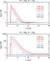 |
Fig. 1 Temporal evolution of atmospheric mass loss in response to stellar flares of different energies. The ratio of the instantaneous mass-loss rate to the quiescent mass-loss rate is shown for input flares ranging from 1031 erg (dark blue) to 1036 erg (dark red). Values are provided at the system’s Hill radius. The top and bottom panels refer to the Earthand sub-Neptune-sized planet, respectively. |
Values of the quiescent mass-loss rate (ṀQ [g s−1]) and the mass-loss increase (∆MF/MQ) obtained from the simulations at the four orbital distances (a = 0.01, 0.1, 0.18, 0.36 AU) for the two activity levels considered (low and high).
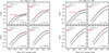 |
Fig. 2 Fractional mass-loss increase per flare (as given by Eq. (5)) as a function of flare energy for both the low-activity (red) and high-activity (blue) cases, each evaluated at four different orbital distances; the 0.18-0.36 AU range brackets the extent of the HZ for the chosen host star. The horizontal lines at the top denote the energy range over which the FFDs were observationally constrained (Loyd et al. 2018, 2023). Our simulations extend to include flare energies up to 1036 erg. The left and right panels refer to the Earth- and sub-Neptune-sized planet, respectively. |
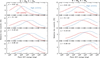 |
Fig. 3 Fractional contributions to the flare-driven mass-loss increase (Eq. (4)) from different flare energies, shown for the high-activity (blue histogram) and low-activity (red) phase, and for four orbital separations. The left and right panels correspond to the Earth-sized planet and the sub-Neptune-sized planet, respectively. |
3.2 Evaporated mass fractions, with and without flares
Using the results in Table 1, we could estimate the cumulative impact of stellar flares by assuming a simplified, two-phase evolution model. In this model, the star undergoes a 1-gigayear-long high-activity phase followed by a 4-gigayear-long low-activity phase (West et al. 2008). Based on the quiescent mass-loss rates from the ATES simulations, we find that, in the absence of flares, the total mass lost over 5 Gyr for the Earth-like planet is 0.65, 0.025, 0.009, and 0.003M⊕ at orbital distances of 0.01, 0.1, 0.18, and 0.36 AU, respectively; for the sub-Neptune, the corresponding values are 1.75, 0.045, 0.015, and 0.004M⊕. When flares are included, the total mass lost increases to approximately 0.68, 0.031, 0.012, and 0.004M⊕ for the Earth-like planet, and 2.02, 0.066, 0.025, and 0.007 M⊕ for the sub-Neptune, at orbital distances of 0.01, 0.1, 0.18, and 0.36 AU, respectively. These values correspond to fractional increases of about 5%, 24%, 33%, and 33% for the Earth-sized planet, and 15%, 47%, 67%, and 75% for the sub-Neptune at the same separations, respectively. We emphasize that the actual values depend on the assumed duration of each activity phase.
When compared to a more simplistic approach that assumes constant evaporation efficiency (e.g., energy-limited escape), our calculations yield systematically lower flare-driven mass-loss increases. Using the energy-limited equation to calculate the mass-loss rate, the increases are approximately 26% and 350% for the low- and high-activity phases, respectively, regardless of planet size or orbital separation. Over 5 Gyr, the total mass lost is 1.79, 0.08, 0.03, and 0.008 M⊕ for the Earth-like planet, and 5.07, 0.152, 0.053, and 0.014 M⊕ for the sub-Neptune, at orbital distances of 0.01, 0.1, 0.18, and 0.36 AU, respectively. At greater distances from the star, where the XUV flux is low, the energylimited model provides a good approximation of the escape rate. However, this is not the case at closer orbital separations.
Our analysis shows that, overall, flares have a modest impact - less than a factor of 2 - on increasing the total mass lost, with the greatest cumulative increase occurring when the planet is in the closest orbit. At larger orbital separations, the total mass lost is much lower due to the reduced quiescent mass-loss rate. However, the relative increase in mass loss between the flaring and non-flaring cases is greater at larger separations.
4 Discussion
4.1 Analytical approach
The main results from our simulations can be summarized as follows: (i) for a given FFD, there exists a characteristic stellar flare energy that maximizes the relative contribution to the mass loss (Fig. 3); (ii) the fractional impact of flares on mass loss is larger at larger orbital distances (Table 1); (iii) regardless of planet size, stellar activity level and orbital distance, flares have a modest contribution to the cumulative mass loss (Table 2). Below, we demonstrate that these somewhat counterintuitive behaviors can be understood by considering the functional dependence of the evaporation efficiency on irradiance, in conjunction with the specific shape of the FFDs.
Without loss of generality, the total atmospheric mass lost within a given time interval can be expressed as ΔM ≈ η 3 FXUV/(4GKρ), where η is the evaporation efficiency, FXUV is the stellar XUV fluence at the planet’s surface, G is the gravitational constant, K accounts for the gravitational potential of the star, and ρ is the planetary mass density (see, e.g., Erkaev et al. 2007; Sanz-Forcada et al. 2011). In energy-limited regime, a large fraction of the absorbed stellar energy is converted into heat and adiabatic expansion, implying ΔM ∝ FXUV, with a nearly constant value for η (typically between 0.1 and 1; see, e.g., Caldiroli et al. 2022; Salz et al. 2016). This approximation is no longer valid at high irradiation (FXUV ≳ 104 erg s−1 cm−2; see, e.g., Murray-Clay et al. 2009), as cooling via radiative recombinations (chiefly Ly-α) becomes very efficient, at the expense of expansion work. In this recombination-limited regime, the evaporation efficiency becomes flux-dependent and decreases with increasing irradiation according to  (Murray-Clay et al. 2009; Owen & Alvarez 2016). We emphasize that planetary gravity is the primary factor in determining the efficiency of atmospheric evaporation (Salz et al. 2016). While Earth-sized and sub-Neptune-sized planets can transition from energy-limited to recombination-limited regimes, gas giants can never be energy-limited. The reader is referred to Caldiroli et al. (2022), and references therein, for an in-depth discussion of the dependence of η on FXUV.
Going back to the impact of a single flare of energy E and duration ΔT, the resulting mass contrast can be written as
 (8)
(8)
We approximated the time-dependent flaring flux, FXUV(t), by averaging it over the flare duration, i.e.,  , where
  is the energy emitted by the quiescent star in the same time interval ΔT. We then defined an average flare efficiency as
  , i.e., the efficiency at average flux. With these definitions the expression for
the mass contrast becomes
 (9)
(9)
For flare energies that are low compared to EQ, the evaporation efficiency remains unchanged from the quiescent state, implying that δM ∝ E. This is true regardless of the evaporation regime, whether it is energy-limited or recombinationlimited. Conversely, if E ≫ EQ, the outflow is most likely recombination-limited, which implies δM ∝ E1/2, since  .
.
As shown in Fig. 4, the transition energy between the δM ∝ E and δM ∝ E1/2 regimes corresponds to the flare energy value where the ratio  begins to differ significantly from unity. Different FFDs and orbital distances result in different transition energies. However, it is important to note that the flare energy at which this transition occurs does not correspond to the flare energy that maximizes the flare’s contribution to mass loss. To understand why, we must examine the interplay between the dependence of δM on the flare energy (E) and the functional shape(s) of the FFD, as follows.
To encompass the full range of behavior between energy-and recombination-limited escape, we expressed the mass contrast as a generic power-law function of energy: δM(E) ∝ Eβ, where β varies between 0.5 and 1. Next, we considered the product E δM dN/dE; a maximum in this quantity corresponds to the characteristic flare energy that maximizes the mass-loss increase due to flares (see Eqs. (4) and (5)). The differential distribution of the number of flares dN/dE scales as ∝ E−α, where α = 1.74(1.61) for low-activity (high-activity) stars. Combing the two expressions above yields E δMdN/dE ∝ Eβ+1-α, which has a maximum for β = 0.74 in the case of low-activity stars, and for β = 0.61 in the case high-activity stars. In practice, as β decreases from 1 to approximately 0.5 as the flare energy increases, the energy-dependent ratio ΔMF/MQ(E) must exhibit a maximum somewhere between Emin and Emax. Critically, this means that neither rare super-flares nor frequent low-amplitude flares have a substantial impact on long-term mass-loss increases due to flares.
Values of the total mass lost in the simplified two-phase evolution of the activity of the star.
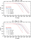 |
Fig. 4 Ratio of the average efficiency of the outflow to the value of the quiescent efficiency as a function of the flare energy for the high-activity phase (blue) and the low-activity phase (red). Efficiencies were calculated using the analytical fitting formula given in Appendix A of Caldiroli et al. (2022). The top and bottom panels correspond to the Earth-sized planet and the sub-Neptune-sized planet, respectively. |
4.2 Simulations with realistic flare time series
The results presented thus far are based on the implicit assumption that atmospheric relaxation times in response to a flare are shorter than the average interval between distinct flares. This implies that the outflowing atmosphere reaches a steady state before the onset of the next flare. However, our simulations indicate that the atmosphere may take several hours to relax following the most energetic flares (see Fig. 1). Consequently, the assumption that flares can be treated independently may not always hold.
This is especially relevant in the high-activity case, where the flaring rate is elevated. For a star in the low-activity regime, the average time interval between low-energy flares (i.e., E ≈ 1030-31 erg; see Fig. 3) is approximately 10-30 hours. This interval is of the same order as the atmospheric relaxation time, which is about 5 hours at an orbital separation of 0.01 AU and approximately 40 hours at 0.36 AU. Thus, for a star in this activity regime, it is reasonable to assume that flares can be treated independently. In the following, we focus on the high-activity phase for the sub-Neptune, for which the cumulative mass loss is expected to be much higher compared to the Earth-like planet.
To test a more realistic scenario, we constructed a template flare time series by sequentially appending multiple flares. Each flare energy was randomly selected from the input FFD, and the flare contrast was constructed as described in Sect. 2. The total duration of the time series was set to 100 days, ensuring that the distribution of flare energies is adequately sampled over the entire range from 1027 to 1036 erg. The resulting time series is illustrated in Fig. 5. We note that for this procedure to be robust, it is necessary to conduct multiple simulations with different random realizations of the time series.
Using ten realizations of the high-activity time series described above as inputs, we repeated the ATES simulations described in the previous sections. The total increase in mass loss was calculated by integrating the mass-loss rate at the Hill radius over the entire duration of the simulation(s).
We find fractional mass-loss increases of 27.61 ± 2.0%, 64.6 ± 6.6%, 82.6 ± 8.5% and 123.7 ± 15.2% at orbital distances of 0.01, 0.1, 0.18 and 0.36 AU, respectively. These values translate to a cumulative mass loss over 5 Gyr of 1.998 ± 0.018 M⊕, 0.064 ± 0.002 M⊕, 0.024 ± 0.0009 M⊕ and 0.008 ± 0.0004 M⊕ at the four orbital distances. The errors are calculated as the standard deviation of the values obtained from the different realizations. The time-series results are consistent with those reported in Tables 1 and 2 within 1-2σ.
We conclude that assuming independent flares is a valid approximation for calculating the integrated contribution of flares to the rise in the mass-loss rate. This is justified by considering the average time interval between flares of the characteristic energy responsible for the greatest increase. From Fig. 3, we find that the peak energy is approximately 1033.5 erg at 0.01 AU and 1035.5 erg at 0.36 AU. These values correspond to average intervals of roughly 20 hours and 10 days, respectively, both of which exceed the corresponding atmospheric relaxation times, which range from about 5 to 40 hours.
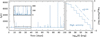 |
Fig. 5 Left: one-year light curves corresponding to the high-activity stellar phase. Right: Flare occurrence rate as a function of energy over the same time interval. |
5 Summary and conclusions
This work represents the first attempt to model the effect of stellar flares on atmospheric evaporation - specifically regarding the H-He envelope - using a time-dependent approach. Our results are qualitatively consistent with the conclusions of do Amaral et al. (2025), who focused on the young M1 star AU Mic and its planetary system, composed of one Earth-sized and two Neptune-sized planets. In their study, the effect of flares was modeled by increasing the quiescent luminosity by an amount corresponding to the average increase induced by flares, with different flare FFDs adopted for various evolutionary epochs. Our analysis confirms their conclusion, that the effects of flaring are more significant at larger orbital separations. Our approach provides physical insight into the underlying reasons for this behavior.
The primary reason for this trend is the fraction of time spent in energy- versus recombination-limited mass-loss regimes. At close orbital separations, the planet is in a recombination-limited mass-loss regime, regardless of whether the star is flaring or not; in this regime, the mass-loss rate scales as the square root of the irradiance. The larger orbital separation case is one in which mass loss is energy-limited, and the mass-loss rate scales linearly with irradiance, even for relatively bright flares. This implies that the large separation case is associated with a larger increase in Ṁ.
Importantly, we demonstrate the existence of a characteristic flare energy that maximizes the fractional contribution to flare-driven mass loss. Even though the actual values of this characteristic energy depend on the orbital distance and the assumed FFD shape, this ensures that neither rare super-flares nor frequent low-amplitude flares have a significant impact on the mass-loss increases caused by stellar flares.
We conclude by emphasizing that the quantitative estimates presented in Tables 1 and 2 are specific to the chosen planetary systems and orbital distances. Overall, we believe that our results can qualitatively apply to other planetary systems - provided they are not gas giants - so long as they experience irradiation levels comparable to those considered in this study.
Quantitatively, the absolute values of Ṁ are systematically lower for the Earth-sized planets than the sub-Neptunes, owing to the higher average density of a terrestrial planet. Assuming an atmospheric mass fraction of 10−3 Mp after the “boil-off” phase following disk dispersal (see, e.g., Owen & Wu 2016; Misener & Schlichting 2021 ; do Amaral et al. 2025), we find that, neglecting flares, an Earth-like planet at 0.18 AU (0.36 AU) would lose its H-He envelope entirely within 168 (600) Myr. When considering the effects of flares, this timescale is reduced to 113 (343) Myr.
Further variations are likely to arise from (i) evolving the planet’s radius in response to mass loss, and (ii) relaxing the assumption that the stellar SED does not vary during flares. We will take these aspects, along with an appropriate grid of planetary radii, masses, and orbital distances, into account in future work.
Acknowledgements
We are grateful to Evgenya Shkolnik and Laura do Amaral for their valuable feedback on an earlier version of this manuscript. We also thank the Editor, Emmanuel Lellouch, for prompting us to extend our original investigation to include Earth-like planets. This research was supported in part from the Michigan Institute for Research in Astrophysics (MIRA). RS acknowledges the support of the ARIEL ASI/INAF agreement no. 2021-5-HH.0 and the support from the European Union - Next Generation EU through the grant no. 2022J7ZFRA - Exo-planetary Cloudy Atmospheres and Stellar High energy (Exo-CASH) funded by MUR - PRIN 2022.
References
- Atri, D., & Mogan, S. R. C. 2021, MNRAS, 500, L1 [Google Scholar]
- Audard, M., Güdel, M., Drake, J. J., & Kashyap, V. L. 2000, ApJ, 541, 396 [Google Scholar]
- Bisikalo, D. V., Cherenkov, A. A., Shematovich, V. I., Fossati, L., & Möstl, C. 2018, Astron. Rep., 62, 648 [Google Scholar]
- Caldiroli, A., Haardt, F., Gallo, E., et al. 2021, A&A, 655, A30 [NASA ADS] [CrossRef] [EDP Sciences] [Google Scholar]
- Caldiroli, A., Haardt, F., Gallo, E., et al. 2022, A&A, 663, A122 [NASA ADS] [CrossRef] [EDP Sciences] [Google Scholar]
- Chadney, J. M., Koskinen, T. T., Galand, M., Unruh, Y. C., & Sanz-Forcada, J. 2017, A&A, 608, A75 [NASA ADS] [CrossRef] [EDP Sciences] [Google Scholar]
- Chen, H., & Rogers, L. A. 2016, ApJ, 831, 180 [Google Scholar]
- Davenport, J. R. A. 2016, ApJ, 829, 23 [Google Scholar]
- Davenport, J. R. A., Hawley, S. L., Hebb, L., et al. 2014, ApJ, 797, 122 [Google Scholar]
- Davenport, J. R. A., Covey, K. R., Clarke, R. W., et al. 2019, ApJ, 871, 241 [Google Scholar]
- do Amaral, L. N. R., Barnes, R., Segura, A., & Luger, R. 2022, ApJ, 928, 12 [NASA ADS] [CrossRef] [Google Scholar]
- do Amaral, L. N. R., Shkolnik, E. L., Loyd, R. O. P., & Peacock, S. 2025, ApJ, 985, 100 [Google Scholar]
- Doyle, L., Ramsay, G., Doyle, J. G., Wu, K., & Scullion, E. 2018, MNRAS, 480, 2153 [Google Scholar]
- Engle, S. G. 2024, ApJ, 960, 62 [NASA ADS] [CrossRef] [Google Scholar]
- Erkaev, N. V., Kulikov, Yu. N., Lammer, H., et al. 2007, A&A, 472, 329 [NASA ADS] [CrossRef] [EDP Sciences] [Google Scholar]
- Feinstein, A. D., Seligman, D. Z., France, K., Gagné, J., & Kowalski, A. 2024, AJ, 168, 60 [Google Scholar]
- France, K., Duvvuri, G., Egan, H., et al. 2020, AJ, 160, 237 [Google Scholar]
- Getman, K. V., & Feigelson, E. D. 2021, ApJ, 916, 32 [NASA ADS] [CrossRef] [Google Scholar]
- Gillet, A., Strugarek, A., & García Muñoz, A. 2025, A&A, 696, A64 [NASA ADS] [CrossRef] [EDP Sciences] [Google Scholar]
- Güdel, M., Audard, M., Skinner, S. L., & Horvath, M. I. 2002, ApJ, 580, L73 [Google Scholar]
- Günther, M. N., Zhan, Z., Seager, S., et al. 2020, AJ, 159, 60 [Google Scholar]
- Hawley, S. L., Fisher, G. H., Simon, T., et al. 1995, ApJ, 453, 464 [NASA ADS] [CrossRef] [Google Scholar]
- Hawley, S. L., Davenport, J. R. A., Kowalski, A. F., et al. 2014, ApJ, 797, 121 [Google Scholar]
- Hazra, G. 2025, Rev. Mod. Plasma Phys., 9, 18 [Google Scholar]
- Hazra, G., Vidotto, A. A., Carolan, S., Villarreal D’Angelo, C., & Manchester, W. 2022, MNRAS, 509, 5858 [Google Scholar]
- Jackson, A. P., Davis, T. A., & Wheatley, P. J. 2012, MNRAS, 422, 2024 [Google Scholar]
- Jackman, J. A. G., Shkolnik, E. L., Loyd, R. O. P., & Richey-Yowell, T. 2024, MNRAS, 533, 1894 [Google Scholar]
- Johnstone, C. P., Bartel, M., & Güdel, M. 2021, A&A, 649, A96 [EDP Sciences] [Google Scholar]
- Ketzer, L., & Poppenhaeger, K. 2023, MNRAS, 518, 1683 [Google Scholar]
- King, G. W., Corrales, L. R., Fernández Fernández, J., et al. 2024, MNRAS, 530, 3500 [Google Scholar]
- Kopparapu, R. K., Ramirez, R., Kasting, J. F., et al. 2013, ApJ, 765, 131 [NASA ADS] [CrossRef] [Google Scholar]
- Kowalski, A. F. 2024, Liv. Rev. Solar Phys., 21, 1 [Google Scholar]
- Kowalski, A. F., Allred, J. C., & Carlsson, M. 2024, ApJ, 969, 121 [NASA ADS] [CrossRef] [Google Scholar]
- Lacy, C. H., Moffett, T. J., & Evans, D. S. 1976, ApJS, 30, 85 [Google Scholar]
- Lammer, H., Selsis, F., Ribas, I., et al. 2003, ApJ, 598, L121 [Google Scholar]
- Lecavelier des Etangs, A., Bourrier, V., Wheatley, P. J., et al. 2012, A&A, 543, L4 [NASA ADS] [CrossRef] [EDP Sciences] [Google Scholar]
- Lee, Y., Dong, C., Pawlowski, D., et al. 2018, Geophys. Res. Lett., 45, 6814 [NASA ADS] [CrossRef] [Google Scholar]
- Lopez, E. D., Fortney, J. J., & Miller, N. 2012, ApJ, 761, 59 [Google Scholar]
- Louca, A. J., Miguel, Y., Tsai, S.-M., et al. 2023, MNRAS, 521, 3333 [NASA ADS] [CrossRef] [Google Scholar]
- Loyd, R. O. P., Shkolnik, E. L., Schneider, A. C., et al. 2018, ApJ, 867, 70 [NASA ADS] [CrossRef] [Google Scholar]
- Loyd, R. O. P., Schneider, P. C., Jackman, J. A. G., et al. 2023, AJ, 165, 146 [NASA ADS] [CrossRef] [Google Scholar]
- Luger, R., Barnes, R., Lopez, E., et al. 2015, Astrobiology, 15, 57 [Google Scholar]
- Malsky, I., Rogers, L., Kempton, E. M. R., & Marounina, N. 2023, Nat. Astron., 7, 57 [Google Scholar]
- Misener, W., & Schlichting, H. E. 2021, MNRAS, 503, 5658 [NASA ADS] [CrossRef] [Google Scholar]
- Murray-Clay, R. A., Chiang, E. I., & Murray, N. 2009, ApJ, 693, 23 [Google Scholar]
- Neupert, W. M. 1968, ApJ, 153, L59 [NASA ADS] [CrossRef] [Google Scholar]
- Osten, R. A., & Wolk, S. J. 2015, ApJ, 809, 79 [NASA ADS] [CrossRef] [Google Scholar]
- Owen, J. E., & Jackson, A. P. 2012, MNRAS, 425, 2931 [Google Scholar]
- Owen, J. E., & Alvarez, M. A. 2016, ApJ, 816, 34 [Google Scholar]
- Owen, J. E., & Wu, Y. 2016, ApJ, 817, 107 [NASA ADS] [CrossRef] [Google Scholar]
- Owen, J. E., & Wu, Y. 2017, ApJ, 847, 29 [Google Scholar]
- Owen, J. E., & Lai, D. 2018, MNRAS, 479, 5012 [Google Scholar]
- Peacock, S., Barman, T., Shkolnik, E. L., et al. 2019, ApJ, 886, 77 [NASA ADS] [CrossRef] [Google Scholar]
- Pietras, M., Falewicz, R., Siarkowski, M., Bicz, K., & Pres, P. 2022, ApJ, 935, 143 [NASA ADS] [CrossRef] [Google Scholar]
- Pye, J. P., Rosen, S., Fyfe, D., & Schröder, A. C. 2015, A&A, 581, A28 [NASA ADS] [CrossRef] [EDP Sciences] [Google Scholar]
- Salz, M., Schneider, P., Czesla, S., & Schmitt, J. H. M. M. 2016, A&A, 585, L2 [NASA ADS] [CrossRef] [EDP Sciences] [Google Scholar]
- Sanz-Forcada, J., Micela, G., Ribas, I., et al. 2011, A&A, 532, A6 [NASA ADS] [CrossRef] [EDP Sciences] [Google Scholar]
- Segura, A., Walkowicz, L. M., Meadows, V., Kasting, J., & Hawley, S. 2010, Astrobiology, 10, 751 [Google Scholar]
- Silverberg, S. M., Kowalski, A. F., Davenport, J. R. A., et al. 2016, ApJ, 829, 129 [NASA ADS] [CrossRef] [Google Scholar]
- Tilley, M. A., Segura, A., Meadows, V., Hawley, S., & Davenport, J. 2019, Astrobiology, 19, 64 [Google Scholar]
- Veronig, A., Temmer, M., Hanslmeier, A., Otruba, W., & Messerotti, M. 2002, A&A, 382, 1070 [NASA ADS] [CrossRef] [EDP Sciences] [Google Scholar]
- West, A. A., Hawley, S. L., Bochanski, J. J., et al. 2008, AJ, 135, 785 [Google Scholar]
- Youngblood, A., France, K., Loyd, R. O. P., et al. 2017, ApJ, 843, 31 [Google Scholar]
- Zhao, Z. H., Hua, Z. Q., Cheng, X., Li, Z. Y., & Ding, M. D. 2024, ApJ, 961, 130 [NASA ADS] [CrossRef] [Google Scholar]
- Zhilkin, A. G., Gladysheva, Y. G., Shematovich, V. I., Tsurikov, G. N., & Bisikalo, D. V. 2024, Astron. Rep., 68, 865 [Google Scholar]
Publicly available at https://github.com/AndreaCaldiroli/ATES-Code
All Tables
Values of the quiescent mass-loss rate (ṀQ [g s−1]) and the mass-loss increase (∆MF/MQ) obtained from the simulations at the four orbital distances (a = 0.01, 0.1, 0.18, 0.36 AU) for the two activity levels considered (low and high).
Values of the total mass lost in the simplified two-phase evolution of the activity of the star.
All Figures
|
Fig. 1 Temporal evolution of atmospheric mass loss in response to stellar flares of different energies. The ratio of the instantaneous mass-loss rate to the quiescent mass-loss rate is shown for input flares ranging from 1031 erg (dark blue) to 1036 erg (dark red). Values are provided at the system’s Hill radius. The top and bottom panels refer to the Earthand sub-Neptune-sized planet, respectively. |
| In the text | |
|
Fig. 2 Fractional mass-loss increase per flare (as given by Eq. (5)) as a function of flare energy for both the low-activity (red) and high-activity (blue) cases, each evaluated at four different orbital distances; the 0.18-0.36 AU range brackets the extent of the HZ for the chosen host star. The horizontal lines at the top denote the energy range over which the FFDs were observationally constrained (Loyd et al. 2018, 2023). Our simulations extend to include flare energies up to 1036 erg. The left and right panels refer to the Earth- and sub-Neptune-sized planet, respectively. |
| In the text | |
|
Fig. 3 Fractional contributions to the flare-driven mass-loss increase (Eq. (4)) from different flare energies, shown for the high-activity (blue histogram) and low-activity (red) phase, and for four orbital separations. The left and right panels correspond to the Earth-sized planet and the sub-Neptune-sized planet, respectively. |
| In the text | |
|
Fig. 4 Ratio of the average efficiency of the outflow to the value of the quiescent efficiency as a function of the flare energy for the high-activity phase (blue) and the low-activity phase (red). Efficiencies were calculated using the analytical fitting formula given in Appendix A of Caldiroli et al. (2022). The top and bottom panels correspond to the Earth-sized planet and the sub-Neptune-sized planet, respectively. |
| In the text | |
|
Fig. 5 Left: one-year light curves corresponding to the high-activity stellar phase. Right: Flare occurrence rate as a function of energy over the same time interval. |
| In the text | |
Current usage metrics show cumulative count of Article Views (full-text article views including HTML views, PDF and ePub downloads, according to the available data) and Abstracts Views on Vision4Press platform.
Data correspond to usage on the plateform after 2015. The current usage metrics is available 48-96 hours after online publication and is updated daily on week days.
Initial download of the metrics may take a while.