| Issue |
A&A
Volume 702, October 2025
|
|
|---|---|---|
| Article Number | A118 | |
| Number of page(s) | 16 | |
| Section | Planets, planetary systems, and small bodies | |
| DOI | https://doi.org/10.1051/0004-6361/202555770 | |
| Published online | 14 October 2025 | |
Discovery of a multi-planet system orbiting the aged Sun-like star HD 224018★
1
INAF – Osservatorio Astrofisico di Torino,
Via Osservatorio 20,
10025
Pino Torinese,
Italy
2
School of Physics & Astronomy, University of Birmingham,
Edgbaston,
Birmingham
B15 2TT,
UK
3
SUPA, School of Physics & Astronomy, University of St Andrews,
North Haugh,
St Andrews,
KY169SS,
UK
4
Centre for Exoplanet Science, University of St Andrews,
North Haugh,
St Andrews,
KY169SS,
UK
5
Space Research and Planetary Sciences, Physics Institute, University of Bern,
Gesellschaftsstrasse 6,
3012
Bern,
Switzerland
6
Sub-department of Astrophysics, University of Oxford,
Keble Rd,
Oxford
OX13RH,
UK
7
Observatoire Astronomique de l’Université de Genève,
Chemin Pegasi 51,
1290
Versoix,
Switzerland
8
Department of Physics, University of Warwick,
Gibbet Hill Road,
Coventry
CV4 7AL,
UK
9
DTU Space, Technical University of Denmark,
Elektrovej 328, 2800 Kgs.
Lyngby,
Denmark
10
University of Southern Queensland, Centre for Astrophysics,
West Street,
Toowoomba,
QLD 4350
Australia
11
Space sciences, Technologies and Astrophysics Research (STAR) Institute, Université de Liège,
Allée du 6 Août 19C,
4000
Liège,
Belgium
12
Astrobiology Research Unit, Université de Liège,
Allée du 6 Août 19C,
4000
Liège,
Belgium
13
Fundación Galileo Galilei - INAF,
Rambla José Ana Fernandez Pérez 7,
38712
Breña Baja,
Tenerife,
Spain
14
Center for Astrophysics I Harvard & Smithsonian,
60 Garden Street,
Cambridge,
MA
02138,
USA
15
Astrobiology Center,
2-21-1 Osawa,
Mitaka,
Tokyo
181-8588,
Japan
16
National Astronomical Observatory of Japan,
2-21-1 Osawa,
Mitaka,
Tokyo
181-8588,
Japan
17
Department of Astronomy, The Graduate University for Advanced Studies (SOKENDAI),
2-21-1 Osawa,
Mitaka,
Tokyo,
Japan
18
INAF – Osservatorio Astronomico di Padova,
Vicolo dell’Osservatorio 5,
35122
Padova,
Italy
19
Dipartimento di Fisica e Astronomia ‘Galileo Galilei’, Università degli Studi di Padova,
Vicolo dell’Osservatorio 3,
35122
Padova,
Italy
20
NASA Ames Research Center,
Moffett Field,
CA
94035,
USA
21
SUPA, Institute for Astronomy, University of Edinburgh,
Blackford Hill,
Edinburgh,
EH9 3HJ,
UK
22
Centre for Exoplanet Science, University of Edinburgh,
Edinburgh,
EH9 3HJ,
UK
23
DTU Space, National Space Institute, Technical University of Denmark,
Elektrovej 328, 2800 Kgs.
Lyngby,
Denmark
24
Affiliate member, Cavendish Laboratory, University of Cambridge,
J J Thomson Avenue,
Cambridge,
CB3 0HE,
UK
25
Astronomy Department of the University of Geneva,
Chemin Pegasi 51,
1290
Versoix,
Switzerland
26
Astrophysics Research Centre, School of Mathematics and Physics, Queen’s University Belfast,
Belfast,
BT7 1NN,
UK
★★ Corresponding author: This email address is being protected from spambots. You need JavaScript enabled to view it.
Received:
2
June
2025
Accepted:
18
August
2025
Abstract
Context. Exoplanetary systems show a large diversity of architectures and planet types. Among the increasing number of exodemographics studies, those exploring correlations between the presence of close-in small planets and cold Jupiters are the object of particular attention.
Aims. In 2016, Kepler/K2 detected a system of two sub-Neptunes transiting the star HD 224018, one of them showing a mono-transit event. In 2017, we began a spectroscopic follow-up with HARPS-N to measure the dynamical masses of the planets using radial velocities, and collected additional transit observations using CHEOPS.
Methods. We measured the fundamental physical parameters of the host star, which is an ‘old Sun’ analogue. We analysed radial velocities and photometric time series, also including data by TESS, to provide precise ephemerides, radii, masses, and bulk densities of the two planets, and possibly modelling their internal structure and composition.
Results. The system turned out to be more crowded than was shown by Kepler/K2. Radial velocities revealed the presence of two additional bodies: a candidate cold companion on an eccentric orbit with a minimum mass nearly half that of Jupiter (eccentricity 0.60−0.08+0.07; semi-major axis 8.6−1.6+1.5 au), and an innermost super-Earth (orbital period 10.6413±0.0028 d; mass 4.1±0.8 M⊕) for which we discovered previously undetected transit events in Kepler/K2 photometry. TESS data revealed a second transit of one of the two companions originally observed by Kepler/K2. This allowed us to constrain its orbital period to a grid of values, the most likely being ~138 days, which would imply a mass less than 9 M⊕ at a 3σ significance level. Given the level of precision of our measurements, we were able to constrain the internal structure and composition of the second-most distant planet from the host star, a warm sub-Neptune with a bulk density of 3.9±0.5 g cm−3.
Conclusions. HD 224018 hosts three close-in transiting planets in the super-Earth-to-sub-Neptune regime, and a candidate cold and eccentric massive companion. Additional follow-up is needed to better characterise the physical properties of the planets and their architecture, and to study the evolutionary history of the system.
Key words: techniques: photometric / techniques: radial velocities / planets and satellites: detection / planets and satellites: fundamental parameters / stars: individual: HD 224018
Based on observations made with the space-based telescopes Kepler/K2, CHEOPS, and TESS, and with the HARPS-N spectrograph mounted on the Italian Telescopio Nazionale Galileo (TNG) operated by the Fundación Galileo Galilei (FGG) of the Istituto Nazionale di Astrofisica (INAF) at the Observatorio del Roque de los Muchachos (La Palma, Canary Islands, Spain).
© The Authors 2025
 Open Access article, published by EDP Sciences, under the terms of the Creative Commons Attribution License (https://creativecommons.org/licenses/by/4.0), which permits unrestricted use, distribution, and reproduction in any medium, provided the original work is properly cited.
This article is published in open access under the Subscribe to Open model. This email address is being protected from spambots. You need JavaScript enabled to view it. to support open access publication.
1 Introduction
Exoplanetary systems exhibit a vast diversity of architectures (Howe et al. 2025), varying in number, size, and mass and in terms of the orbital configuration of the planets. Among this diversity, we find: tightly packed systems with small planets in inner coplanar or mutually inclined orbits; systems with giant planets in wide, and sometimes highly eccentric orbits; and systems with both close-in small planets and outer gas giants. Various architectures arise from the different initial conditions in protoplanetary discs, as well as from the stochastic processes inherent in planetary formation and evolution (e.g. Mordasini et al. 2012; Wu et al. 2019; Wang et al. 2022). Whether the populations of close-in small planets (with mass 1 M⊕ < mp < 20 M⊕ and semi-major axis a ≲ 0.4 au) and cold Jupiters (i.e. outer gas giants with mp = 0.3–13 MJup and semi-major axis a = 1–10 au) are related and to what extent, and whether any possible correlation depends on stellar parameters, such as metallicity and mass, is currently a subject of lively debate (see e.g. Bryan et al. 2019; Bonomo et al. 2023; Bryan & Lee 2024, 2025; Van Zandt & Petigura 2024; Bonomo et al. 2025).
Among multi-planet systems with small planets in shortperiod orbits, those in which planets have distinct properties are especially intriguing, such as equilibrium temperatures and/or radii, in particular below and above the ‘radius valley’, a marked deficit in the number of planets with sizes between about 1.5 and 2 R⊕ in the radius distribution of small exoplanets (e.g. Fulton et al. 2017). This radius gap reflects a dichotomy in planetary composition, in that it separates smaller Earth-like planets and super-Earths from larger sub-Neptunes, which are possibly ice-rich planets and/or planets surrounded by a substantial gas envelope. It may be explained invoking different formation processes, including orbital migration mechanisms (e.g. Venturini et al. 2020), of super-Earths and sub-Neptunes (for instance, inside and outside the water snowline for rocky super-Earths and ice-rich sub-Neptunes, respectively; see e.g. Parc et al. 2024; Shibata & Izidoro 2025) and/or post-formation processes, such as atmospheric photo-evaporation (e.g. Owen & Wu 2017; Van Eylen et al. 2018), core-powered mass loss (e.g. Ginzburg et al. 2018; Gupta & Schlichting 2019), and erosion caused by giant impacts (e.g. Reinhardt et al. 2022). The above-mentioned formation and evolutionary mechanisms are expected to produce characteristic trends in the location of the radius valley as a function of the orbital period or stellar irradiation level (e.g. Lopez & Rice 2018; Martinez et al. 2019; Van Eylen et al. 2021). To investigate these trends, it is crucial to determine accurate and precise bulk densities of small planets with relatively long orbital periods (P > 30 d) corresponding to lower insolation levels. However, the number of well-studied planets with P > 30 d remains relatively scarce compared to those with shorter periods. This is due to transit detection and follow-up surveys, such as TESS and CHEOPS, being biased towards short-period planets, and to the difficulties in detecting the Doppler radial velocity (RV) signals induced on their host star, often hampered or mimicked by those due to stellar activity.
The Sun-like star HD224018 (EPIC246214735), located at 106 pc, was initially identified as an interesting target for RV follow-up as four transit-like features were detected in the light curve collected by the space-based telescope Kepler/K2 (hereafter K2). Three transits are produced by a sub-Neptune with a period of P~37 d, while the fourth signal is a monotransit of another sub-Neptune-sized companion on a wider orbit. We observed HD 224018 with the high-resolution spectrograph HARPS-N for seven years with the aim of measuring the masses of the two companions, and concurrently better constraining the orbit of the outermost one. In parallel with our RV campaign, we collected additional photometric transits of the innermost sub-Neptune with the CHaracterising ExOPlanets Satellite (CHEOPS; Benz et al. 2021). HD224018 was also observed by the Transiting Exoplanet Survey Satellite (TESS; Ricker et al. 2015), increasing the sample of the detected transits. In this study we present the results from the RV and photometric follow-up. Our data allowed us to detect two additional companions in the system: a short-period transiting Earth-size planet, and a candidate cold Jupiter on a wide and highly eccentric orbit. Our findings make HD 224018 an interesting target for exoplanet population studies, in that it would enrich the demographics of multi-planet systems with an eccentric and massive outer planet encircling a compact group of small-size companions.
The paper is structured as follows. In Sect. 2 we describe the datasets used in this study. We report the fundamental physical parameters of the host star in Sect. 3. In Sect. 4 we show the results of a frequency analysis of the RVs, and in Sect. 5 we present the outcome of the analysis of transit photometry. In Sect. 6 we discuss the analysis of spectroscopic stellar activity diagnostics and of the RV systematics. Based on that, we define the RV dataset used for a joint spectroscopic-photometric modelling, which is described in Sect. 7. In Sect. 8 we discuss the possible internal structure and composition of the only planet for which we were able to precisely measure the mass and radius. We conclude with a summary and discussion on future perspectives in Sect. 9.
2 Observations and data reduction
2.1 Photometry
2.1.1 K2
HD 224018 was observed by K2 during campaign 12 from 15 December 2016 to 4 March 2017. We analysed the 30-min cadence light curve1 that was extracted following the methodology described by Vanderburg & Johnson (2014). The modelling of all the transit signals detected in the photometric time series was performed on the light curve, which was detrended2 using the publicly available python package wδtan3 (Hippke et al. 2019), using the built-in cosine function (i.e. a sum of sines and cosines, with an iterative clipping of 2σ outliers until convergence). The final detrended light curve was obtained after masking all the identified transits (see Sect. 5 for details). Fig. 1 shows the undetrended K2 light curve, a preliminary version of the detrended photometric time series, and a close-up view of the three naked-eye visible transit features. These are the signals that triggered our spectroscopic follow-up, which started a few months after the detection by K2. At a first look, three of these events appear to be produced by one companion with a periodicity of ~37 days, but the first one is actually deeper and due to the superposition of at least two distinct transits of a similar depth. That second event corresponds to the mono-transit of a second planet-sized companion.
2.1.2 CHEOPS
Due to its photometric precision, the CHEOPS space telescope has been successfully used in the discovery (e.g. Bonfanti et al. 2021; Wilson et al. 2022; Osborn et al. 2023) and timing (e.g. Borsato et al. 2021; Nascimbeni et al. 2023; Borsato et al. 2024) of small exoplanets. To refine the ephemerides of the planet that transits the host every ~37 days after a gap of 4.5 years from K2 observations, we covered two consecutive transit events with CHEOPS on 2-3 September 2021 and 9-10 October 2021 as part of the CH_PR220007 program. Our visits have an observational efficiency of 90.2 and 75.7%, respectively, and a cadence of 60 s, resulting in 1645 total frames.
We processed both visits with the latest version of the CHEOPS Data Reduction Pipeline (DRP v14, Hoyer et al. 2020), which performs calibrations (e.g. dark current, flat field correction, and event flagging) and corrections (background flux, cosmic rays, and smearing from nearby objects) on the raw data. The CHEOPS DRP performs aperture photometry on the images using 25 circular apertures, with radii ranging from 15 to 40 pixels. In this study, the light curves that have the lowest RMS scatter are those produced with the 26 and 23 pixel apertures, respectively. We utilised the PYCHEOPS package4 (Maxted et al. 2022) to retrieve basis vectors corresponding to instrumental metrics (e.g. the target x- and y-centroid position, background value, and CHEOPS spacecraft roll angle). We used the Juliet python package (Espinoza et al. 2019) to detrend the light curve, by simultaneously fitting the transit model alongside a linear noise model constructed from the CHEOPS basis vectors.
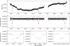 |
Fig. 1 K2 light curve of HD 224018. Upper panel : undetrended photometric time series. Middle panel : first version of the detrended and flattened light curve, provided in the public archive (Vanderburg & Johnson 2014; the curve analysed in this work is shown in Fig. 3). Naked-eye visible transit signals are marked with dashed red lines. Lower panels : zoomed-in views showing details of the transit-like signals. The morphology of the first one looks more complex as it is the superposition of two transits. |
2.1.3 TESS
HD 224018 was observed by TESS in sectors 42 (20 August-16 September 2021) and 70 (20 September-15 October 2023). For our analysis we used the simple aperture photometry (SAP; Twicken et al. 2010; Morris et al. 2020) light curve, provided by the TESS Science Processing Operations Center (SPOC; Jenkins et al. 2016; Caldwell et al. 2020) pipeline, with a cadence of 120 and 200 s for the two sectors, respectively. The SAP light curve was not corrected for dilution because of a negligible contamination level within the photometric aperture. The quality of the data is not comparable to that of K2 and CHEOPS. Nonetheless, we used TESS data to improve the precision on the ephemerides of the ~37 d transiting planet. Sector 70 turned out to be important for the presence of a second transit of the other companion identified in the K2 light curve.
2.2 Spectroscopy
We observed HD 224018 with the HARPS-N spectrograph (Cosentino et al. 2012) from 6 August 2017 to 10 October 2023, collecting 206 spectra that were reduced with the standard Data Reduction Software (DRS) pipeline (version 3.0.1), and accessed through the Data Analysis Center for Exoplanets (DACE)5 Web platform. The median and standard deviation of the spectra signal-to-noise ratio (S/N) are ~75 and 10, respectively, as measured at a reference wavelength of 5500 Â. The target was placed on fibre A of the spectrograph, while fibre B was simultaneously illuminated with a Fabry-Pérot etalon used as a calibration source. The RVs and the activity diagnostics full width at half maximum (FWHM), bisector span (BIS), and contrast were calculated from the cross-correlation function (CCF; Baranne et al. 1996) using a template mask for a star of spectral type G8, and have a median internal error, σRV, of 1.51 ms−1 and median systemic RV of –62870.84 ms−1.
2.3 High-resolution imaging
On the night of 14 August 2017, HD 224018 was observed with the NESSI speckle imager (Scott 2019), mounted on the 3.5 m WIYN telescope at Kitt Peak. NESSI acquires data in two bands centred at 562 and 832 nm simultaneously using highspeed electron-multiplying CCDs (EMCCDs). We collected and reduced the data following the procedures described in Howell et al. (2011). The resulting reconstructed image achieved a contrast of Δmag~5.7 at a separation of 1" in the 832 nm band (see Fig. B.1), and no secondary sources were detected.
3 Stellar fundamental parameters
HD 224018 is a G dwarf star located 106.1 ± 0.2 pc away (Bailer-Jones et al. 2021). We derived the atmospheric stellar parameters by analysing the HARPS-N spectra: the effective temperature (Teff), surface gravity (log g), metallicity ([Fe∕H]), microturbulence (ξ), and projected rotational velocity (v sin i⋆). The former three parameters were derived via two methods, and we adopt their inverse-variance weighted average as our final parameters, while the last two parameters are method-specific. First, we applied the curve-of-growth method ARES+MOOG. In this method, we measured the equivalent widths of neutral and ionised iron lines from the co-added spectrum. Assuming local thermodynamic equilibrium and employing the Kurucz Atlas 9 plane parallel model atmospheres (Kurucz 1993), we fitted for the atmospheric parameters using radiative transfer modelling. The details of the method are described in Sousa (2014). To ensure accuracy, we corrected the surface gravity following Mortier et al. (2014). Systematic errors were added in quadrature following Sousa et al. (2011). We find that Teff = 5813 ± 69 K, log g = 4.33 ± 0.11 dex, and [Fe/H]= 0.05 ± 0.05. This method additionally measures the microturbulence, ξ. Following a second method, we used SPC (Spectral Parameter Classification - Buchhave et al. 2012, 2014), a technique based on spectral synthesis. Each individual spectrum was analysed, and the final results were obtained by taking a weighted average of the individual spectra using the S/N values for the weights. To ensure accuracy in the surface gravity measurement, YY isochrones (Yi et al. 2001) were used as an extra constraint. We find that Teff = 5755 ± 50 K, log g = 4.28 ± 0.10 dex, and [m/H]= –0.03 ± 0.08. This method additionally measures the projected rotational velocity.
Individual chemical abundances are useful for interior modelling of exoplanets. For these purposes, we measured the magnesium and silicon abundances in addition to the already derived iron abundance. The abundances were calculated using ARES+MOOG (see Mortier et al. 2013 for details). We find that [Mg/H] = 0.04±0.05 and [Si/H] = 0.08±0.05. This is consistent with the solar-type nature of this star.
To measure the stellar radius, mass, and age, we used the effective temperature and metallicity derived from the spectra. We performed an analysis based on isochrones and evolutionary tracks, using both the Dartmouth and MIST stellar models (Dotter et al. 2008; Dotter 2016). Next to the spectroscopic input, we used photometric apparent magnitudes in eight bands [Johnson B and V, 2MASS and WISE], and the Gaia DR3 parallax (Lindegren et al. 2021; Gaia Collaboration 2023). The analysis was performed four separate times, allowing for each combination of the individual spectroscopic results and the different stellar models. More details can be found in Mortier et al. (2020). By adopting as final parameters and errors the median and 16th-84th percentiles of the combined posterior distributions, we found  ,
,  , and an age of
  Gyr.
Gyr.
We also modelled the MIST evolutionary tracks along with the stellar spectral energy distribution (SED) in a differential evolution Markov chain Monte Carlo (MC) Bayesian framework through the EXOFASTv2 tool (Eastman 2017; Eastman et al. 2019); see Naponiello et al. (2025) for more details. To this end, we imposed Gaussian priors on the Gaia DR3 parallax as well as on the Teff and [Fe/H] from our spectroscopically derived parameters. To sample the SED, we used the Tycho–2 BT and VT, APASS Johnson B and V, and Sloan g′, r′, i′ magnitudes, the 2MASS near-infrared J, H, and Ks magnitudes, and the WISE W1, W2, and W3 infrared magnitudes (Table 1). The stellar SED and its best fit are shown in Fig. B.2. From the medians and 16th-84th percentiles of the posteriors we derived  , R⋆ = 1.147 ± 0.028 R⊙, and an age of
  Gyr, which fully agree with the previous solution. Given the larger, and thus more conservative, uncertainties, we chose these as our reference stellar parameters in this work. The derived surface gravity,
  , is fully consistent with the spectroscopic value, but more precise.
Finally, we derived Galactic space velocities for HD 224018 using the co-ordinates, proper motions, parallax, and RV from Gaia DR3. We followed the formulation by Johnson & Soderblom (1987) to calculate the U, V, and W heliocentric velocity components and its errors. The velocities are defined in the directions of the Galactic centre, Galactic rotation (using the right-hand system), and north Galactic pole, respectively. The solar motion was not subtracted. From these velocities we assigned membership probabilities using a MC approach and following the Reddy et al. (2006) formalism. Kinematically, this star is found to have a probability of 88.4 ± 0.5% of being a thick disc star and 11.1 ± 0.5% of being a thin disc star. The age and chemical composition of this star point more to a thin disc star, but could still be consistent with a thick disc star. All our derived stellar parameters are summarised in Table 1.
Stellar parameters of HD224018 (EPIC246214735; TIC 248608315).
4 Frequency analysis of radial velocities
We used the generalised Lomb-Scargle periodogram (GLS; Zechmeister & Kürster 2009) for a first identification of significant periodical signals in the original RV time series and pre-whitened RV residuals. Looking at the original RV time series (see the upper left panel of Fig. B.3), there is a clear long-term trend for which it is not possible to confirm a periodicity, because the data do not cover a sufficiently long time span. The GLS periodogram of the original dataset is shown in the first panel of Fig. 2. We used a Keplerian with a leastsquares best-fit period of P =10998 d and eccentricity of e=0.7 for a first pre-whitening, to search for other periodic signals. The GLS periodograms from the second to the fourth pre-whitened dataset are shown in Fig. 2. We adopted a Keplerian with zero eccentricity as a model for the iterative pre-whitening. The false alarm probability (FAP) levels of the main peaks were evaluated through a bootstrap (with replacement) simulations. The analysis of the pre-whitened RV residuals reveals the existence of a significant signal at P = 36.58 ± 0.07 days (semi-amplitude K = 1.9 ± 0.2 ms−1 ), which is a period very close to that of the transit signal detected by K2. Therefore, it is safe to conclude that it is produced by the same companion. We also found a signal at P = 10.636 ± 0.007 d with a FAP of 1.54% (semi-amplitude K = 1.1 ± 0.2 ms−1), and its nature is unveiled in Sect. 5. After a third and last pre-whitening, the periodogram reveals a peak at P = 44.7 ± 0.2 d with a large FAP (~10%). We lack additional evidence to support the hypothesis that this corresponds to the stellar rotation period or any other astrophysical signal, such as an additional planet, and given its high FAP value we do not consider it further in our analysis.
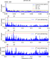 |
Fig. 2 GLS periodograms (in frequency and period) of the HARPS-N original radial velocities ( upper panel ) and residuals. These were calculated through an iterative pre-whitening. Red triangles mark the peaks with the highest power. False alarm probability levels are indicated by horizontal dashed lines. |
5 Photometric data analysis
5.1 Improving the sensitivity to transit detection in K2 data
In Sect. 2.1.1 we showed the existence of two companions orbiting HD 224018 thanks to the K2 observation of transits. For one of them, we detected the counterpart signal in the RV time series, while for the other companion only a mono-transit is revealed. We used the python package wδtan (Hippke et al. 2019) to perform an optimal detrending of the K2 and TESS light curves, with the goals of preserving the actual shape of the transit profiles after removing trends from time-series data, and search for possibly undetected transits of short-period planets, in particular of a third body that could be responsible for the 10.6-day signal found in the RVs. We found that among several of the available detrending algorithms provided by wδtan, the cosine method produced the best results in terms of signal detection efficiency (SDE)6. After it was applied a first time to the original light curve, we used the transit least squares (TLS) algorithm (Hippke & Heller 2019) to constrain the properties of the signal due to the –36.6-d companion (which is detected with an SDE=25.9), and masked the corresponding three transits, also adopting a time interval wide enough to mask the overlapped transits. Then, we detrended the masked light curve, and running TLS on the flattened dataset led to a more significant detection of the –36.6-d signal, boosting the SDE to a value of 29.1. After masking the transits again on the better detrended light curve, we searched for additional transit-like signals with TLS. We found the main peak in the periodogram at P=21.28 days (SDE=8.1), i.e. at exactly twice the period of the 10.64 day signal detected in the RV data. We interpret this result as evidence that the RV signal is associated with a short-period transiting companion, and the low SDE peak revealed at –21 days is due to the low S/N of the transits, with some of them not identified by TLS. After identifying the transits of the 10.6-day companion with TLS, we masked all the transit signals in the K2 data to perform a last and more accurate detrending of the original light curve. That resulted in an increase in the SDE for the P=21.28 day signal (SDE=9.4). The SDE of the 10.64 d transit signal is –8. Further application of the TLS algorithm did not show other significant peaks in the periodogram.
A summary of the results from the analysis described above is provided in Fig. 3. Our fine-tuned detrending of the K2 light curve allowed us to identify very shallow transits of the 10.64-day companion first detected in the RV, which were missed by an initial blind search (these are shown in Fig. B.6). It turns out that the first transit of the 10.64 day companion occurred while the other two companions were also transiting, so that K2 actually observed a triple transit event. Following an order based on their distance from the host star, we identify the companions with orbital periods 10.64 and 36.6 days, and the one showing a mono-transit as HD 224018 b, HD 224018 c, and HD 224018 d, respectively. Our final measurements of radii and masses for these companions, described in Sect. 7, justify that they are identified as planets.
5.2 CHEOPS and TESS light curves
CHEOPS and TESS light curves were detrended with wōtan using the same set-up and steps adopted for K2 data. We note that the first transit of HD 224018 c observed by CHEOPS occurred in a gap of the TESS data in sector 42. As was mentioned, TESS observations of sector 70 contain one transit, increasing to six the number of recorded transits for this planet. In Sect. 7 we report the detection of a second transit of HD 224018 d in TESS data of sector 70.
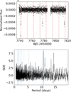 |
Fig. 3 Results from the detrending of the K2 light curve with wotan. Upper panel : detrended light curve, with the epochs of the transits of HD 224018 b indicated by vertical dashed lines. Lower panel : TLS periodogram after masking the 36.6 day transits and the mono-transit, and restricting the search to orbital periods shorter than 19.7 days. The main peak is found at 10.64 days. Individual transits with very low S/N transits are shown in Fig. B.6, demonstrating how a fine-tuned detrending was crucial for their detection. |
6 Spectroscopic data analysis
6.1 Activity diagnostics analysis
Figure 4 shows the time series and the corresponding GLS periodograms of three activity indicators extracted from the HARPS-N spectra: the CCF-derived BIS and CCF area, given by the product FWHM-contrast, and the S index. We used the CCF area as a diagnostic, instead of the individual FWHM and contrast time series, because their significant anti-correlation is likely due to long-term changes in the instrument focus (for more details, refer to Collier Cameron et al. 2019). We do not find significant periodicities in the BIS time series, while the periodograms of the CCF area and S index show significant peaks at ~1255 and ~515 days, respectively, with low FAPs determined through a bootstrap analysis.
6.2 Identification of RV systematics with YARARA and SCALPELS
We processed the HARPS-N spectra time series through YARARA, a post-processing data-driven methodology aiming to extract as much as possible information contained in a highresolution spectrum. The final goal of YARARA is to provide an independent measurement of the RV time series, either measured by a CCF using a tailored line selection (Cretignier et al. 2020) or line-by-line RVs (Cretignier et al. 2023) following the prescription of Dumusque (2018), but also providing activity indicators (Cretignier et al. 2024). Because of its limitation due to the data quality, we decided not to use YARARA to measure the RVs. Nevertheless, the analysis revealed interesting results that are reported in Appendix A, together with more details on the method.
Motivated by the need to understand the contribution of stellar activity in the RV observations, we used the SCALPELS method devised by Collier Cameron et al. (2021). SCALPELS decorrelates for spectral line-shape changes in CCFs, induced by stellar variability, while preserving the Doppler shift component that we can use for planet searches. To obtain reliable detections of planets from the SCALPELS ‘shift’ component of the RVs, we used TWEAKS (Anna John et al. 2022, 2023), a workflow that integrates SCALPELS with the trans-dimensional nested sampling algorithm called KIMA (Faria et al. 2016). SCALPELS sets out by creating an orthogonal basis with the coefficients of the first few leading principal components of shape-induced CCF fluctuations. The raw RVs are then projected on this basis to generate a time series of shape-induced RV variations (Fig. 5). The basis vectors (U-vectors) representing the shape components identified by SCALPELS are then used for stellar activity decorrelation using the KIMA. KIMA employs diffusive nested sampling (Brewer 2014) to sample the posterior distributions for each of the orbital parameters by modelling the RV data with a sum of up to Np Keplerian functions. KIMA also perform simultaneous Gaussian process analysis to counteract any leakage of shift-like stellar activity signal during the SCALPELS U-vector decorrelation.
To ensure a clean set of basis vectors, SCALPELS uses the median absolute deviation (MAD) to discard anomalous observations that may generate spurious basis functions (See Section 3.2 in Collier Cameron et al. 2021). For HD 224018, this resulted in the rejection of 29 spectra from the initial sample of 206, leaving 177 useful data points to use in our analysis. After the rejection of bad rows, the columns of the right singular matrix U were re-ordered in the descending order of their contribution to improve the chi-squared and the Bayesian information criterion (BIC) in a planet-free model. The number of decorrelation vectors that minimise the BIC in our case is three. The time series of RVs and the SCALPELS decorrelation basis vectors are shown in Fig. 5, and published online at the CDS (see Data Availability section). As more planet signals are fitted, the relative significance of the basis vectors could vary because the U vectors are not necessarily orthogonal to the parts of the signal that Keplerians are now fitting out.
For HD 224018, two basis vectors were excluded from further runs in order to avoid over-fitting, since they did not significantly contribute to the three-planet model. Therefore, we only included U0, as it may help mitigate an instrumental effect or a long-term activity cycle. Apparently, there is a long-term effect manifesting itself as a slightly asymmetric change, as it is also observed in the time series of the CCF area (cfr. with Fig. 4). Otherwise, the star does not display signs of strong intrinsic variability in terms of changes in the shape of the CCF. There is very little shape-driven RV variability, suggesting little spot activity or photometric effect due to facular contrast. Later in this paper, we directly use the RV dataset defined with SCALPELS to perform the joint analysis discussed in Sect. 7.
7 Photometric and spectroscopic joint analysis
We measured the fundamental planetary parameters by performing joint MC modelling of RV and photometric light curves, using the nested sampler and Bayesian inference tool MULTINEST V3.10 (e.g. Feroz et al. 2019), through the pyMULTINEST wrapper (Buchner et al. 2014). The MC set-up is characterised by 500 live points, a sampling efficiency of 0.5, and an evidence tolerance of 0.5. Radial velocity and transit signals were modelled using the python packages radvel7 (Fulton et al. 2018) and pytransit8 (Parviainen 2015), respectively.
The analysed dataset include the 177 RVs defined through the analysis with SCALPELS, and the detrended K2, CHEOPS, and TESS light curves. We modelled transit signals of HD 224018 b only in K2 data because their S/N is too low to make them detectable in the other datasets. We also included the SCALPELS decorrelation basis vector U0, with the linear correlation coefficient α0 as a free parameter.
In summary, our RV model includes four Keplerians to fit the RV Doppler signals, and the correction of systematics with SCALPELS. For the photometric part, we included three transiting signals for the three innermost companions. For the eccentricities of the three transiting planets we adopted a Gaussian prior N(μ = 0, σ = 0.1) based on the results of Van Eylen et al. (2019), while for the candidate companion HD 224018 e, instead of fitting directly the eccentricity, ee, and the argument of periastron, ω*,e, we used the alternative parameterisation  and
and  (Anderson et al. 2011). Concerning the light curves, we adopted a quadratic law for the limb darkening, and fitted the coefficients u1 and u2 (two sets, one in common for K2 and CHEOPS, one for TESS) using the parametrisation for coefficients q1 and q2 given by Kipping (2010) (see Eq. (15) and (16) therein). We also introduced offsets, γ, and constant jitters, σjit, as free parameters for both the spectroscopic and photometric dataset, and for each instrument. The jitter values were added in quadrature to the RV and light curve internal uncertainties. Considering the long cadence of the K2 light curve, in order to mitigate morphological distortions when fitting the transit light curves in this dataset (see Kipping 2010), we used a photometric oversampling factor of 15.
The total number of fitted parameters of our model is equal to 40. We adopted uniform priors for all of them with the exception of the eccentricities of the three transiting companions, as mentioned above, and the stellar density, ρ*, which we used in place of the ac/R⋆ ratio at each step of the MC sampling (e.g. Sozzetti et al. 2007), for which we adopted a Gaussian prior based on the result of Sect. 3. The complete list of priors and best-fit results, for free and derived parameters, is given in Table 2.
The main results of the joint RV and photometric modelling can be summarised as follows. For HD 224018 b, we measure a mass of 4.1 ±0.8 M⊕, but the radius (as well as the bulk density) cannot be determined with either accuracy or precision (rb =  R⊕, with 3σ error bars given in parentheses). Individual transits are shown in Fig. B.6. Some are not visible, such as the first and second transit, because of the very low S/N. No significant transit time variations are detected within the uncertainties of the retrieved transit times. HD 224018 c is a sub-Neptune for which we measure precise mass, radius, and bulk density:
  M⊕,
M⊕,  R⊕, and ρc = 4.0
 g cm−3. For HD 224018 d, our analysis reveals that the TESS data of Sector 70 likely contains a second transit. The marginal posterior of Pd is shown in Fig. B.4, together with the grid of possible orbital periods derived from the relation
  ), where q is an integer representing a specific harmonic of the orbital period, and T0,K2 and T0,TESS are the transit midpoints of the two observed transits. From this distribution we constrained the orbital period to be
  days. Fig. B.4 shows that Pd = 138.07 days is the most likely orbital period among the predicted values (corresponding to the integer q = 18), and the large asymmetry of the 1σ error bars was determined by the second most likely period in the grid, Pd = 165.69 days (corresponding to the integer q = 15). The statistical preference for Pd = 138.07 days was determined from the information contained in the RVs, from which we measured a semi-amplitude of the Doppler signal associated with planet d with a significance level of 2.6σ, Kd=0.52
 m s−1. This corresponds to a planetary mass of md=4.2
 M⊕. The radius of this planet is comparable to that of planet c, and the resulting bulk density of HD 224018 d is
  g cm−3. Nonetheless, given the low statistical significance of Kd, ours should be assumed to be a tentative detection of the RV signal, and 3σ upper limits should be considered for the mass and density, 9.0 M⊕ and 4.2 g cm−3, respectively. Indeed, whether the real orbital period of HD 224018 d is close to 138 days (with implications for the mass and bulk density measurements) must be confirmed with the detection of at least one more transit event. For the outermost candidate companion, we did not observe a full orbital cycle; thus, we cannot constrain the orbital period and semimajor axis well with our current RV time series (
 days;
days;  au). However, the spectroscopic orbit has a significantly high eccentricity (
 ), and the Doppler semi-amplitude is well constrained (
 ms−1), corresponding to a minimum mass of nearly 0.5 MJup. Therefore, our solution shows that HD 224018 e is compatible with being a cold Jupiter, although additional spectroscopic follow-up is needed to better constrain its minimum mass and orbital architecture. We note that the applied RV correction using the first SCALPELS basis vector, U0, is significant at a level of ~2σ (
 ), and that the applied correction has preserved the signal of the wide-orbit planetary candidate signal, supporting it having an astrophysical origin. The GLS periodogram of the RV residuals, after subtracting all the spectroscopic signals that are included in our model, confirms the presence of a statistically insignificant main peak at ~45 days, as is discussed in Sect. 4.
We show in Figs. 6 and B.5 the transit light curves of HD 224018 b, c, and d, and in Fig. 7 the Doppler RV signals. The epochs of mid transit are summarised in Table B.1. Fig. B.3 shows the full RV time series and the four Keplerian model, after applying the SCALPELS correction. The cartoon in Fig. B.7 shows part of the K2 light curve at the epochs when the three innermost planets where transiting together. Fig. 8 shows a massradius diagram including planets with precise mass measurements, the three transiting planets in the HD 224018 system, and theoretical curves representative of some compositional models.
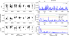 |
Fig. 4 Time series and periodograms of the spectroscopic activity diagnostics BIS, CCF area (FWHM-contrast), and S index. First column : time series of the activity indexes. The average values have been subtracted from each dataset. Second column : GLS periodograms. Red triangles indicate peak values. The horizontal lines correspond to levels of FAPs determined through a bootstrap analysis. |
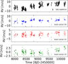 |
Fig. 5 Radial velocity time series selected with SCALPELS as our definitive dataset (upper panel). Radial velocities projection onto the first three basis vectors calculated with SCALPELS are shown in the other panels. |
Priors and best-fit values for the free and derived parameters from the joint RV and light curve modelling.
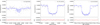 |
Fig. 6 Transits of the three innermost planets in the HD 224018 system as observed by K2. For planets b and c, the transits are phase-folded to their corresponding orbital periods. The blue lines represent the best-fit transit models. The shaded blue area indicates the 1σ uncertainty in the transit depths (rp/R*)2. The O-C data points are the residuals of the best-fit models. |
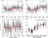 |
Fig. 7 Doppler signals of HD 224018 induced by the four planetary companions. For planets b, c, and d, phase-folded data are shown. The best-fit models are indicated by a red curve. For HD 224018 d we used the maximum likelihood values of the Keplerian parameters (Kd = 0.43 ms−1; Pd = 138.07 d; Tc = 2457741.745 BJD; ed = 0.018; ω*,d = 2.74 rad). For HD 224018 e the RV time series is shown because the orbit is not fully characterised. The error bars include the uncorrelated jitter added in quadrature to the RV uncertainties. |
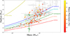 |
Fig. 8 Mass-radius diagram for all planets with radii R < 4 R⊕ characterised by HARPS-N (coloured dots, with the colour scale based on the precision of mass measurement). Non-coloured dots correspond to all other planets with R < 4 R⊕ and a mass precision higher than 30% as measured by means of RVs. The three transiting planets orbiting HD 224018 are indicated with green squares. Green dots indicate the location of Earth and Venus. Some compositional theoretical curves are also plotted (Zeng et al. 2019). |
8 Internal structure analysis of HD 224018 c
As a next step, we used the plaNETic9 framework (Egger et al. 2024) to infer the internal structure of HD 224018 c. We focused only on this planet because it is the one for which we could measure a precise mass and radius. We did also run models for planets b and d, but given the low precision in radius and mass the inferred posteriors are very close to the chosen priors. This effect is even stronger for planet d, as here also the orbital period and therefore the planet’s equilibrium temperature is not well constrained. plaNETic uses a neural network trained on the forward model of BICEPS (Haldemann et al. 2024) as a surrogate model in combination with a full grid accept-reject sampling scheme, allowing for a fast and reliable characterisation of the internal structure of observed exoplanets.
For this purpose, the planet was modelled as a combination of an inner core (Fe, S), a mantle (oxidised Si, Mg, and Fe), and a volatile layer (uniformly mixed H/He and water). As the connection between the composition of planets and their host stars is still highly debated in the literature (e.g. Thiabaud et al. 2015; Adibekyan et al. 2021; Michel et al. 2020), we ran models using three different compositional priors, one assuming the planetary Si/Mg/Fe ratios equal the ones of the host star (Thiabaud et al. 2015), one assuming the planet is iron-enriched compared to the host star (Adibekyan et al. 2021), and one independent of the stellar abundances, whereby the planetary Si/Mg/Fe ratios are sampled using a uniform prior. Additionally, we also used two different priors for the water content of the planet, resulting in a water-rich scenario as would be expected if the planet had formed outside the ice line, and a water-poor scenario in accordance with a formation inside the ice line. More details on framework and chosen priors can be found in Egger et al. (2024).
Table 3 and Figure 9 show the most important internal structure parameters for HD 224018 c. If we assume the planet formed in an environment in which water could only be accreted through the accreted gas (i.e. inside the water ice line), we infer a rather tightly constrained envelope of around 1% in total planet mass that is almost purely made up of H/He. On the other hand, for a water-prior consistent with a formation scenario outside the ice line we find that a wide range of envelope mass fractions is possible, with a preference for more massive envelopes. Generally, these envelopes show high water mass fractions.
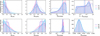 |
Fig. 9 Posterior distributions for internal structure parameters of HD 224018 c: mass fractions, with respect to the total planet mass, of (i) the inner core (wcore); (ii) the mantle (wmantle); (iii) the envelope layers (wenvelope); mass fraction of H/He in the envelope (1-Zenvelope); mass fraction of water in the envelope layer (Zenvclopc). Dotted lines show the priors, and dashed vertical lines the median values of the posteriors. Different colours are used for different compositional priors for the planetary Si/Mg/Fe ratios, which were chosen to be stellar (purple), iron-enriched compared to the host star (pink), or freely sampled using a uniform prior (blue). The top row shows models generated using a water prior in agreement with a formation outside the ice line, the bottom row ones with a formation inside the ice line. |
Results of the internal structure modelling for HD 224018 c.
9 Summary and conclusions
We have presented the discovery and first characterisation of a multi-planet system orbiting the 7.0 Gyr old Sunanalogue HD 224018. The system includes three planet-size transiting companions, observed to transit simultaneously in one circumstance (Fig. B.7). A fourth outermost family member is detected only in the RVs. The innermost planet, b (Pb =10.6413±0.0028 d), was initially detected from the analysis of the RVs alone, and its transits were then revealed in the K2 data, although they are shallow and characterised by a low S/N, preventing us from carrying out accurate and precise modelling. Our analysis reveals that it has a mass of mb=4.1±0.8 M⊕ and a radius of
  R⊕ (3σ error bars are given in parentheses). The planet’s location on the mass-radius diagram indicates that the planet’s internal composition spans from that of the Earth down to a bare 100% iron core.
The second planet in order of distance from the host star is a warm sub-Neptune, and it is the only member of the system for which we can provide a precise mass and radius (relative uncertainties of 1.6 and 2.1%, respectively), with a bulk density of 3.9±0.5 g cm−3. That allowed us to model the interior structure of HD 224018 c, with the results that depend on whether the planet formed inside or outside the water ice line.
The third companion, HD 224018 d, was first discovered thanks to a mono-transit observed in the K2 light curve. We found that there is a likely second transit in TESS data, and our analysis shows that the most likely orbital period is ~138 days. While this paper was under review, a new TESS light curve was issued (Sector 92), which will be analysed in detail in a future study. Only a transit of planet c is detected, while a transit event possibly imputable to planet d is not seen. This non-detection is in agreement with the prediction assuming an orbital period of 138.07 days. The new TESS observations seem to rule out an orbital period of 146.19 days, which is the value immediately following 138.07 days in the grid of possible periods compatible with the transits observed by K2 and TESS (see Fig. B.6). The planet is a sub-Neptune with a well-measured radius, rd=2.4±0.1 R⊕, and we derived the dynamical mass  M⊕ (<9 M⊕ at 99.7% significance level). The analysis of the available data shows that HD 224018 d has a very similar size to HD 224018 c, but the precision on the mass measurement prevents us from constraining its internal structure and composition.
For the fourth and outermost member of the system, the current dataset does not allow us to constrain its wide orbit well, although this appears to be highly eccentric ( ). We present HD 224018 e as a candidate giant companion with a minimum mass nearly half that of Jupiter, a semi-major axis of
  au, and the periastron at ~3.5 au. The Gaia DR3 renormalised unit weight error (RUWE) of HD 224018 is 0.92 (single-star solution). The sensitivity curves to companions on wide orbits (Fig. B.8) show that massive Jupiters at a~2-3 au, and brown dwarfs at a>5 au can be ruled out, and that a planet with a mass of ~0.5 MJup is well below the detectability threshold. A RV follow-up is required to establish if HD 224018 e belongs to the population of cold (a ~ 1–10 au) or ultra-cold (a ≳ 10 au) Jupiters. In the former case, it will add to the current sample of only 15 systems with transiting inner low-mass planets (m < 20 M⊕) and outer cold Jupiters (Bonomo et al. 2025); it may be one of the very few systems with multiple inner small planets in the presence of a high-eccentricity (e ≳ 0.4) cold Jupiter.
Acknowledgements
The HARPS-N project was funded by the Prodex Program of the Swiss Space Office (SSO), the Harvard University Origin ofLife Initiative (HUOLI), the Scottish Universities Physics Alliance (SUPA), the University of Geneva, the Smithsonian Astrophysical Observatory (SAO), the Italian National Astrophysical Institute (INAF), University of St. Andrews, Queen’s University Belfast, and University of Edinburgh. We used data from the European Space Agency (ESA) mission Gaia (https://www.cosmos.esa.int/gaia), processed by the Gaia Data Processing and Analysis Consortium (DPAC, https://www.cosmos.esa.int/web/gaia/dpac/consortium). Funding for the DPAC has been provided by national institutions, in particular the institutions participating in the Gaia Multilateral Agreement. Kepler was competitively selected as the 10th Discovery mission. Funding for the Kepler/K2 missions were provided by NASA’s Science Mission Directorate. CHEOPS is an ESA mission in partnership with Switzerland with contributions to the payload and the ground segment from Austria, Belgium, France, Germany, Hungary, Italy, Portugal, Spain, Sweden and the UK. We used data by the TESS mission. Funding for the TESS mission is provided by the NASA Explorer Program. We acknowledge the use of public TOI Release data from pipelines at the TESS Science Office and at the TESS Science Processing Operations Center. Resources supporting this work were provided by the NASA High-End Computing (HEC) Program through the NASA Advanced Supercomputing (NAS) Division at Ames Research Center for the production of the SPOC data products. We used The Data & Analysis Center for Exoplanets (DACE), which is a facility based at the University of Geneva (CH) dedicated to extrasolar planets data visualisation, exchange and analysis. DACE is a platform of the Swiss National Centre of Competence in Research (NCCR) PlanetS, federating the Swiss expertise in Exoplanet research. The DACE platform is available at https://dace.unige.ch. A.M. acknowledges funding from a UKRI Future Leader Fellowship, grant number MR/X033244/1 and a UK Science and Technology Facilities Council (STFC) small grant ST/Y002334/1. A.C.C acknowledges support from STFC consolidated grant number ST/V000861/1 and UKRI/ERC Synergy Grant EP/Z000181/1 (REVEAL). L.M. acknowledges support from the European Union- NextGenerationEU (PRIN MUR 2022 20229R43BH). R.T. acknowledges the Head of Department of Physics, the University of Cambridge, and the Carlsberg Foundation for supporting this research. C.A.W. would like to acknowledge support from the UK Science and Technology Facilities Council (STFC, grant number ST/X00094X/1). We acknowledge support from the INAF Large Grant 2023 ‘EXODEMO’, and from the Swiss National Science Foundation within the framework of the NCCR PlanetS under grants 51NF40_182901 and 51NF40_205606.
Data availability
RVs and activity indexes, with the S index calibrated on the Mount Wilson scale (Wilson 1968), are available at the CDS via https://cdsarc.cds.unistra.fr/viz-bin/cat/J/A+A/702/A118
Appendix A YARARA applied to HARPS-N spectra
The pipeline begins from the S1D order-merged spectra level produced by the official DRS v3.0.1 (Dumusque et al. 2021), with a minimal requirement of prior information during the processing in order to allow an easy scalability with different instruments. The extracted information contains as much as activity indicators, than stellar atmospheric parameters (Cretignier et al. 2024), even if the final goal of the method is to provide an independent measurement of the RV time series, either measured by a CCF using a tailored line selection (Cretignier et al. 2020) or line-by-line RVs (Cretignier et al. 2023) following the prescription of (Dumusque 2018). The analysis with YARARA revealed that an offset visible in the CCF area time series around BJD 2 458 500 is mainly due to the blue part of the spectra, a result similar to the one obtained on the solar telescope (see the orange curve in Fig. A1 of Klein et al. 2024) and likely related to an instrumental systematic on the detector. The RVs of HD 224018 appear to be affected by an offset around the same epoch, which is spotted by the analysis performed with SCALPELS discussed in Sect. 6.2 (see Fig. 5). We can exclude that the overall long-term variability seen in the RV time series, at a level of a few ms−1, is determined by systematics related to the long-term stability of the HARPS-N spectrograph, like instrumental RV drift, instrument warm-up, or power failure, which have been found to produce offsets no larger than 2 m s−1 (Meunier et al. 2024). This leads us to conclude that the longterm trend observed in RVs has mainly an astrophysical origin, such as the presence of a long-term substellar companion.
Appendix B Additional plots and tables
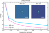 |
Fig. B.1 HD 224018 observed with the NESSI speckle imager mounted on the 3.5 m WIYN telescope at Kitt Peak. |
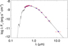 |
Fig. B.2 Stellar SED. The broad band measurements from the Tycho, APASS Johnson, Sloan, 2MASS and WISE magnitudes are shown in red, and the corresponding theoretical values with blue circles. The best-fit model is displayed with a black solid line. |
Epochs of mid transits for the three innermost planets in the system.
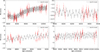 |
Fig. B.3 Time series of the RVs. The measurements are indicated by red dots, and our best-fit spectroscopic model is over-plotted with a black line. The upper left panel shows the full time series, the other plots show zoomed-in views to better appreciate the agreement between the observations and best-fit model. The error bars include the uncorrelated jitter added in quadrature to the RV uncertainties. |
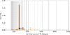 |
Fig. B.4 Posterior of the orbital period Pd obtained from a joint RV and photometry modelling. The width of each bin is ~5 days. The best-fit value (±1σ) is indicated with a black asterisk. Dashed vertical lines correspond to possible orbital periods from a grid of discrete Pd values calculated from the transit midpoints from K2 and TESS. |
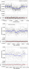 |
Fig. B.5 Transits of HD224018c in CHEOPS, and TESS photometry (first and second panels). Transit of HD 224018 d observed by TESS (lower panel). Residuals (O-C) after subtracting the best-fit transit models are shown for each transit. |
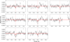 |
Fig. B.6 Individual transits of HD 224018 b in the K2 light curve, following the order specified in the top right label of each panel. The best-model fit is represented by the red line. Note that the light curve has been cleared of both the systematics and the transits of the other two planets. |
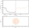 |
Fig. B.7 Snapshot of the triple transit of planet b, c, and d as seen by K2 at the end of 2016. This artistic representation has been created with the software tango (https://github.com/oscaribv/tango). |
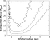 |
Fig. B.8 Gaia DR3 sensitivity to companions of a given mass as a function of the orbital semi-major axis orbiting HD 224018. Dashed, dashed-dotted, and long-dashed lines correspond to iso-probability curves for 80, 90, and 99% probability of a companion of given properties to produce RUWE>0.92. |
References
- Adibekyan, V., Dorn, C., Sousa, S. G., et al. 2021, Science, 374, 330 [NASA ADS] [CrossRef] [Google Scholar]
- Anderson, D. R., Collier Cameron, A., Hellier, C., et al. 2011, ApJ, 726, L19 [NASA ADS] [CrossRef] [Google Scholar]
- Anna John, A., Collier Cameron, A., & Wilson, T. G. 2022, MNRAS, 515, 3975 [Google Scholar]
- Anna John, A., Collier Cameron, A., Faria, J. P., et al. 2023, MNRAS, 525, 1687 [Google Scholar]
- Bailer-Jones, C. A. L., Rybizki, J., Fouesneau, M., Demleitner, M., & Andrae, R. 2021, AJ, 161, 147 [Google Scholar]
- Baranne, A., Queloz, D., Mayor, M., et al. 1996, A&AS, 119, 373 [NASA ADS] [CrossRef] [EDP Sciences] [Google Scholar]
- Benz, W., Broeg, C., Fortier, A., et al. 2021, Exp. Astron., 51, 109 [Google Scholar]
- Bonfanti, A., Delrez, L., Hooton, M. J., et al. 2021, A&A, 646, A157 [EDP Sciences] [Google Scholar]
- Bonomo, A. S., Dumusque, X., Massa, A., et al. 2023, A&A, 677, A33 [NASA ADS] [CrossRef] [EDP Sciences] [Google Scholar]
- Bonomo, A. S., Naponiello, L., Pezzetta, E., et al. 2025, A&A, 700, A126 [NASA ADS] [CrossRef] [EDP Sciences] [Google Scholar]
- Borsato, L., Piotto, G., Gandolfi, D., et al. 2021, MNRAS, 506, 3810 [NASA ADS] [CrossRef] [Google Scholar]
- Borsato, L., Degen, D., Leleu, A., et al. 2024, A&A, 689, A52 [NASA ADS] [CrossRef] [EDP Sciences] [Google Scholar]
- Brewer, B.J. 2014, arXiv e-prints [arXiv:1411.3921] [Google Scholar]
- Bryan, M. L., & Lee, E. J. 2024, ApJ, 968, L25 [NASA ADS] [CrossRef] [Google Scholar]
- Bryan, M. L., & Lee, E. J. 2025, ApJ, 982, L7 [Google Scholar]
- Bryan, M. L., Knutson, H. A., Lee, E. J., et al. 2019, AJ, 157, 52 [Google Scholar]
- Buchhave, L. A., Latham, D. W., Johansen, A., et al. 2012, Nature, 486, 375 [NASA ADS] [Google Scholar]
- Buchhave, L. A., Bizzarro, M., Latham, D. W., et al. 2014, Nature, 509, 593 [Google Scholar]
- Buchner, J., Georgakakis, A., Nandra, K., et al. 2014, A&A, 564, A125 [NASA ADS] [CrossRef] [EDP Sciences] [Google Scholar]
- Caldwell, D. A., Tenenbaum, P., Twicken, J. D., et al. 2020, Res. Notes Am. Astron. Soc., 4, 201 [Google Scholar]
- Collier Cameron, A., Mortier, A., Phillips, D., et al. 2019, MNRAS, 487, 1082 [Google Scholar]
- Collier Cameron, A., Ford, E. B., Shahaf, S., et al. 2021, MNRAS, 505, 1699 [NASA ADS] [CrossRef] [Google Scholar]
- Cosentino, R., Lovis, C., Pepe, F., et al. 2012, SPIE Conf. Ser., 8446, 84461V [Google Scholar]
- Cretignier, M., Dumusque, X., Allart, R., Pepe, F., & Lovis, C. 2020, A&A, 633, A76 [NASA ADS] [CrossRef] [EDP Sciences] [Google Scholar]
- Cretignier, M., Dumusque, X., Aigrain, S., & Pepe, F. 2023, A&A, 678, A2 [NASA ADS] [CrossRef] [EDP Sciences] [Google Scholar]
- Cretignier, M., Hara, N. C., Pietrow, A. G. M., et al. 2024, MNRAS, 535, 2562 [NASA ADS] [CrossRef] [Google Scholar]
- Cutri, R. M., Wright, E. L., Conrow, T., et al. 2021, VizieR Online Data Catalog: II/328 [Google Scholar]
- Cutri, R. M., Skrutskie, M. F., van Dyk, S., et al. 2003, VizieR Online Data Catalog: II/246 [Google Scholar]
- Dotter, A. 2016, ApJS, 222, 8 [Google Scholar]
- Dotter, A., Chaboyer, B., Jevremovic, D., et al. 2008, ApJS, 178, 89 [NASA ADS] [CrossRef] [Google Scholar]
- Dumusque, X. 2018, A&A, 620, A47 [NASA ADS] [CrossRef] [EDP Sciences] [Google Scholar]
- Dumusque, X., Cretignier, M., Sosnowska, D., et al. 2021, A&A, 648, A103 [NASA ADS] [CrossRef] [EDP Sciences] [Google Scholar]
- Eastman, J. 2017, Astrophysics Source Code Library [record ascl:1710.003] [Google Scholar]
- Eastman, J. D., Rodriguez, J. E., Agol, E., et al. 2019, arXiv e-prints [arXiv:1907.09480] [Google Scholar]
- Egger, J. A., Osborn, H. P., Kubyshkina, D., et al. 2024, A&A, 688, A223 [NASA ADS] [CrossRef] [EDP Sciences] [Google Scholar]
- Espinoza, N., Kossakowski, D., & Brahm, R. 2019, MNRAS, 490, 2262 [Google Scholar]
- Faria, J. P., Haywood, R. D., Brewer, B. J., et al. 2016, A&A, 588, A31 [NASA ADS] [CrossRef] [EDP Sciences] [Google Scholar]
- Feroz, F., Hobson, M. P., Cameron, E., & Pettitt, A. N. 2019, Open J. Astrophys., 2, 10 [Google Scholar]
- Fulton, B. J., Petigura, E. A., Howard, A. W., et al. 2017, AJ, 154, 109 [Google Scholar]
- Fulton, B. J., Petigura, E. A., Blunt, S., & Sinukoff, E. 2018, PASP, 130, 044504 [Google Scholar]
- Gaia Collaboration (Prusti, T., et al.) 2016, A&A, 595, A1 [NASA ADS] [CrossRef] [EDP Sciences] [Google Scholar]
- Gaia Collaboration (Brown, A. G. A., et al.) 2021, A&A, 649, A1 [NASA ADS] [CrossRef] [EDP Sciences] [Google Scholar]
- Gaia Collaboration (Vallenari, A., et al.) 2023, A&A, 674, A1 [NASA ADS] [CrossRef] [EDP Sciences] [Google Scholar]
- Ginzburg, S., Schlichting, H. E., & Sari, R. 2018, MNRAS, 476, 759 [Google Scholar]
- Gupta, A., & Schlichting, H. E. 2019, MNRAS, 487, 24 [Google Scholar]
- Haldemann, J., Dorn, C., Venturini, J., Alibert, Y., & Benz, W. 2024, A&A, 681, A96 [NASA ADS] [CrossRef] [EDP Sciences] [Google Scholar]
- Henden, A. A., Templeton, M., Terrell, D., et al. 2016, VizieR Online Data Catalog: AAVSO Photometric All Sky Survey (APASS) DR9 (Henden+, 2016), VizieR On-line Data Catalog: II/336 [Google Scholar]
- Hippke, M., & Heller, R. 2019, A&A, 623, A39 [NASA ADS] [CrossRef] [EDP Sciences] [Google Scholar]
- Hippke, M., David, T. J., Mulders, G. D., & Heller, R. 2019, AJ, 158, 143 [Google Scholar]
- Høg, E., Fabricius, C., Makarov, V. V., et al. 2000, A&A, 355, L27 [Google Scholar]
- Howe, A. R., Becker, J. C., Stark, C. C., & Adams, F. C. 2025, AJ, 169, 149 [Google Scholar]
- Howell, S. B., Everett, M. E., Sherry, W., Horch, E., & Ciardi, D. R. 2011, AJ, 142, 19 [Google Scholar]
- Hoyer, S., Guterman, P., Demangeon, O., et al. 2020, A&A, 635, A24 [NASA ADS] [CrossRef] [EDP Sciences] [Google Scholar]
- Jenkins, J. M., Twicken, J. D., McCauliff, S., et al. 2016, SPIE Conf. Ser., 9913, 99133E [Google Scholar]
- Johnson, D. R. H., & Soderblom, D. R. 1987, AJ, 93, 864 [Google Scholar]
- Kipping, D. M. 2010, MNRAS, 408, 1758 [Google Scholar]
- Klein, B., Aigrain, S., Cretignier, M., et al. 2024, MNRAS, 531, 4238 [Google Scholar]
- Kurucz, R. L. 1993, SYNTHE Spectrum Synthesis Programs and Line Data (Cambridge, Mass.: Smithsonian Astrophysical Observatory) [Google Scholar]
- Lindegren, L., Klioner, S. A., Hernández, J., et al. 2021, A&A, 649, A2 [EDP Sciences] [Google Scholar]
- Lopez, E. D., & Rice, K. 2018, MNRAS, 479, 5303 [NASA ADS] [CrossRef] [Google Scholar]
- Martinez, C. F., Cunha, K., Ghezzi, L., & Smith, V. V. 2019, ApJ, 875, 29 [Google Scholar]
- Maxted, P. F. L., Ehrenreich, D., Wilson, T. G., et al. 2022, MNRAS, 514, 77 [NASA ADS] [CrossRef] [Google Scholar]
- Meunier, N., Lagrange, A. M., Dumusque, X., & Sulis, S. 2024, A&A, 687, A303 [NASA ADS] [CrossRef] [EDP Sciences] [Google Scholar]
- Michel, A., Haldemann, J., Mordasini, C., & Alibert, Y. 2020, A&A, 639, A66 [NASA ADS] [CrossRef] [EDP Sciences] [Google Scholar]
- Mordasini, C., Alibert, Y., Klahr, H., & Henning, T. 2012, A&A, 547, A111 [NASA ADS] [CrossRef] [EDP Sciences] [Google Scholar]
- Morris, R. L., Twicken, J. D., Smith, J. C., et al. 2020, Kepler Data Processing Handbook: Photometric Analysis (USA: Kepler Science Document) [Google Scholar]
- Mortier, A., Santos, N. C., Sousa, S. G., et al. 2013, A&A, 558, A106 [NASA ADS] [CrossRef] [EDP Sciences] [Google Scholar]
- Mortier, A., Sousa, S. G., Adibekyan, V. Z., Brandäo, I. M., & Santos, N. C. 2014, A&A, 572, A95 [NASA ADS] [CrossRef] [EDP Sciences] [Google Scholar]
- Mortier, A., Zapatero Osorio, M. R., Malavolta, L., et al. 2020, MNRAS, 499, 5004 [Google Scholar]
- Naponiello, L., Bonomo, A. S., Mancini, L., et al. 2025, A&A, 693, A7 [NASA ADS] [CrossRef] [EDP Sciences] [Google Scholar]
- Nascimbeni, V., Borsato, L., Zingales, T., et al. 2023, A&A, 673, A42 [NASA ADS] [CrossRef] [EDP Sciences] [Google Scholar]
- Osborn, H. P., Nowak, G., Hébrard, G., et al. 2023, MNRAS, 523, 3069 [NASA ADS] [CrossRef] [Google Scholar]
- Owen, J. E., & Wu, Y. 2017, ApJ, 847, 29 [Google Scholar]
- Parc, L., Bouchy, F., Venturini, J., Dorn, C., & Helled, R. 2024, A&A, 688, A59 [NASA ADS] [CrossRef] [EDP Sciences] [Google Scholar]
- Parviainen, H. 2015, MNRAS, 450, 3233 [Google Scholar]
- Reddy, B. E., Lambert, D. L., & Allende Prieto, C. 2006, MNRAS, 367, 1329 [Google Scholar]
- Reinhardt, C., Meier, T., Stadel, J. G., Otegi, J. F., & Helled, R. 2022, MNRAS, 517, 3132 [NASA ADS] [CrossRef] [Google Scholar]
- Ricker, G. R., Winn, J. N., Vanderspek, R., et al. 2015, J. Astron. Teles. Instrum. Syst., 1, 014003 [Google Scholar]
- Scott, N. J. 2019, AAS/Div. Extreme Sol. Syst. Abstracts, 15, 330.15 [Google Scholar]
- Shibata, S., & Izidoro, A. 2025, ApJ, 979, L23 [Google Scholar]
- Sousa, S. G. 2014, in Determination of Atmospheric Parameters of B (Berlin: Springer), 297 [Google Scholar]
- Sousa, S. G., Santos, N. C., Israelian, G., Mayor, M., & Udry, S. 2011, A&A, 533, A141 [NASA ADS] [CrossRef] [EDP Sciences] [Google Scholar]
- Sozzetti, A., Torres, G., Charbonneau, D., et al. 2007, ApJ, 664, 1190 [Google Scholar]
- Thiabaud, A., Marboeuf, U., Alibert, Y., Leya, I., & Mezger, K. 2015, A&A, 574, A138 [NASA ADS] [CrossRef] [EDP Sciences] [Google Scholar]
- Twicken, J. D., Clarke, B. D., Bryson, S. T., et al. 2010, Proc. SPIE, 7740, 774023 [NASA ADS] [CrossRef] [Google Scholar]
- Van Eylen, V., Agentoft, C., Lundkvist, M. S., et al. 2018, MNRAS, 479, 4786 [Google Scholar]
- Van Eylen, V., Albrecht, S., Huang, X., et al. 2019, AJ, 157, 61 [Google Scholar]
- Van Zandt, J., & Petigura, E. A. 2024, AJ, 168, 268 [Google Scholar]
- Vanderburg, A., & Johnson, J. A. 2014, PASP, 126, 948 [Google Scholar]
- Van Eylen, V., Astudillo-Defru, N., Bonfils, X., et al. 2021, MNRAS, 507, 2154 [NASA ADS] [Google Scholar]
- Venturini, J., Guilera, O. M., Haldemann, J., Ronco, M. P., & Mordasini, C. 2020, A&A, 643, L1 [NASA ADS] [CrossRef] [EDP Sciences] [Google Scholar]
- Wang, S., Kanagawa, K. D., & Suto, Y. 2022, ApJ, 932, 31 [Google Scholar]
- Wilson, O. C. 1968, ApJ, 153, 221 [Google Scholar]
- Wilson, T. G., Goffo, E., Alibert, Y., et al. 2022, MNRAS, 511, 1043 [NASA ADS] [CrossRef] [Google Scholar]
- Wu, D.-H., Zhang, R. C., Zhou, J.-L., & Steffen, J. H. 2019, MNRAS, 484, 1538 [Google Scholar]
- Yi, S., Demarque, P., Kim, Y.-C., et al. 2001, ApJS, 136, 417 [Google Scholar]
- Zechmeister, M., & Kürster, M. 2009, A&A, 496, 577 [CrossRef] [EDP Sciences] [Google Scholar]
- Zeng, L., Jacobsen, S. B., Sasselov, D. D., et al. 2019, Proc. Natl. Acad. Sci., 116, 9723 [Google Scholar]
Hereafter we use the term ‘detrended’ to refer to a light curve which has been flattened and normalised after removing temporal trends.
For detrending the data we used the following wōtan keywords: window length=1.2, break tolerance=0.5, and robust=True.
All Tables
Priors and best-fit values for the free and derived parameters from the joint RV and light curve modelling.
All Figures
|
Fig. 1 K2 light curve of HD 224018. Upper panel : undetrended photometric time series. Middle panel : first version of the detrended and flattened light curve, provided in the public archive (Vanderburg & Johnson 2014; the curve analysed in this work is shown in Fig. 3). Naked-eye visible transit signals are marked with dashed red lines. Lower panels : zoomed-in views showing details of the transit-like signals. The morphology of the first one looks more complex as it is the superposition of two transits. |
| In the text | |
|
Fig. 2 GLS periodograms (in frequency and period) of the HARPS-N original radial velocities ( upper panel ) and residuals. These were calculated through an iterative pre-whitening. Red triangles mark the peaks with the highest power. False alarm probability levels are indicated by horizontal dashed lines. |
| In the text | |
|
Fig. 3 Results from the detrending of the K2 light curve with wotan. Upper panel : detrended light curve, with the epochs of the transits of HD 224018 b indicated by vertical dashed lines. Lower panel : TLS periodogram after masking the 36.6 day transits and the mono-transit, and restricting the search to orbital periods shorter than 19.7 days. The main peak is found at 10.64 days. Individual transits with very low S/N transits are shown in Fig. B.6, demonstrating how a fine-tuned detrending was crucial for their detection. |
| In the text | |
|
Fig. 4 Time series and periodograms of the spectroscopic activity diagnostics BIS, CCF area (FWHM-contrast), and S index. First column : time series of the activity indexes. The average values have been subtracted from each dataset. Second column : GLS periodograms. Red triangles indicate peak values. The horizontal lines correspond to levels of FAPs determined through a bootstrap analysis. |
| In the text | |
|
Fig. 5 Radial velocity time series selected with SCALPELS as our definitive dataset (upper panel). Radial velocities projection onto the first three basis vectors calculated with SCALPELS are shown in the other panels. |
| In the text | |
|
Fig. 6 Transits of the three innermost planets in the HD 224018 system as observed by K2. For planets b and c, the transits are phase-folded to their corresponding orbital periods. The blue lines represent the best-fit transit models. The shaded blue area indicates the 1σ uncertainty in the transit depths (rp/R*)2. The O-C data points are the residuals of the best-fit models. |
| In the text | |
|
Fig. 7 Doppler signals of HD 224018 induced by the four planetary companions. For planets b, c, and d, phase-folded data are shown. The best-fit models are indicated by a red curve. For HD 224018 d we used the maximum likelihood values of the Keplerian parameters (Kd = 0.43 ms−1; Pd = 138.07 d; Tc = 2457741.745 BJD; ed = 0.018; ω*,d = 2.74 rad). For HD 224018 e the RV time series is shown because the orbit is not fully characterised. The error bars include the uncorrelated jitter added in quadrature to the RV uncertainties. |
| In the text | |
|
Fig. 8 Mass-radius diagram for all planets with radii R < 4 R⊕ characterised by HARPS-N (coloured dots, with the colour scale based on the precision of mass measurement). Non-coloured dots correspond to all other planets with R < 4 R⊕ and a mass precision higher than 30% as measured by means of RVs. The three transiting planets orbiting HD 224018 are indicated with green squares. Green dots indicate the location of Earth and Venus. Some compositional theoretical curves are also plotted (Zeng et al. 2019). |
| In the text | |
|
Fig. 9 Posterior distributions for internal structure parameters of HD 224018 c: mass fractions, with respect to the total planet mass, of (i) the inner core (wcore); (ii) the mantle (wmantle); (iii) the envelope layers (wenvelope); mass fraction of H/He in the envelope (1-Zenvelope); mass fraction of water in the envelope layer (Zenvclopc). Dotted lines show the priors, and dashed vertical lines the median values of the posteriors. Different colours are used for different compositional priors for the planetary Si/Mg/Fe ratios, which were chosen to be stellar (purple), iron-enriched compared to the host star (pink), or freely sampled using a uniform prior (blue). The top row shows models generated using a water prior in agreement with a formation outside the ice line, the bottom row ones with a formation inside the ice line. |
| In the text | |
|
Fig. B.1 HD 224018 observed with the NESSI speckle imager mounted on the 3.5 m WIYN telescope at Kitt Peak. |
| In the text | |
|
Fig. B.2 Stellar SED. The broad band measurements from the Tycho, APASS Johnson, Sloan, 2MASS and WISE magnitudes are shown in red, and the corresponding theoretical values with blue circles. The best-fit model is displayed with a black solid line. |
| In the text | |
|
Fig. B.3 Time series of the RVs. The measurements are indicated by red dots, and our best-fit spectroscopic model is over-plotted with a black line. The upper left panel shows the full time series, the other plots show zoomed-in views to better appreciate the agreement between the observations and best-fit model. The error bars include the uncorrelated jitter added in quadrature to the RV uncertainties. |
| In the text | |
|
Fig. B.4 Posterior of the orbital period Pd obtained from a joint RV and photometry modelling. The width of each bin is ~5 days. The best-fit value (±1σ) is indicated with a black asterisk. Dashed vertical lines correspond to possible orbital periods from a grid of discrete Pd values calculated from the transit midpoints from K2 and TESS. |
| In the text | |
|
Fig. B.5 Transits of HD224018c in CHEOPS, and TESS photometry (first and second panels). Transit of HD 224018 d observed by TESS (lower panel). Residuals (O-C) after subtracting the best-fit transit models are shown for each transit. |
| In the text | |
|
Fig. B.6 Individual transits of HD 224018 b in the K2 light curve, following the order specified in the top right label of each panel. The best-model fit is represented by the red line. Note that the light curve has been cleared of both the systematics and the transits of the other two planets. |
| In the text | |
|
Fig. B.7 Snapshot of the triple transit of planet b, c, and d as seen by K2 at the end of 2016. This artistic representation has been created with the software tango (https://github.com/oscaribv/tango). |
| In the text | |
|
Fig. B.8 Gaia DR3 sensitivity to companions of a given mass as a function of the orbital semi-major axis orbiting HD 224018. Dashed, dashed-dotted, and long-dashed lines correspond to iso-probability curves for 80, 90, and 99% probability of a companion of given properties to produce RUWE>0.92. |
| In the text | |
Current usage metrics show cumulative count of Article Views (full-text article views including HTML views, PDF and ePub downloads, according to the available data) and Abstracts Views on Vision4Press platform.
Data correspond to usage on the plateform after 2015. The current usage metrics is available 48-96 hours after online publication and is updated daily on week days.
Initial download of the metrics may take a while.