| Issue |
A&A
Volume 702, October 2025
|
|
|---|---|---|
| Article Number | A195 | |
| Number of page(s) | 9 | |
| Section | The Sun and the Heliosphere | |
| DOI | https://doi.org/10.1051/0004-6361/202556069 | |
| Published online | 24 October 2025 | |
Solar flares versus solar energetic particle events: Probabilistic projections to extreme events
1
Sodankylä Geophysical Observatory, 99600, University of Oulu, Sodankylä, Finland
2
Space Physics and Astronomy Research Unit, P.O.Box 8000 90014 University of Oulu, Oulu, Finland
3
Max-Planck-Institut für Sonnensystemforschung, 37077 Göttingen, Germany
4
University of Graz, Institute of Physics, 8010 Graz, Austria
⋆ Corresponding author: This email address is being protected from spambots. You need JavaScript enabled to view it.
Received:
24
June
2025
Accepted:
16
August
2025
Abstract
Aims. Terrestrial cosmogenic isotope records yield that extreme solar particle events (ESPEs) are relatively rare, occurring approximately once every 1500 years. In contrast, stellar observations show that superflares on solar-like stars might be significantly more frequent. This discrepancy raises the question of whether superflares and ESPEs are different manifestations of the same underlying phenomenon or whether they represent fundamentally distinct phenomena.
Methods. We analysed the conditional probability of a solar particle event occurring in relation to a solar flare with a given peak flux in soft X-rays, based on the observed statistics for the last 45 years. The probability was parametrised and extrapolated to extreme events to evaluate the probabilistic relationship between ESPEs and superflares.
Results. We found that the ESPEs may not be directly related to superflares but are likely produced by moderately strong flares if other coronal and interplanetary factors accidentally become favourable. ESPEs tend to occur during periods of weak-to-moderate solar activity. Thus, the difference in the occurrence rates of ESPEs and superflares can be naturally explained by the lack of a direct relation between these types of phenomena.
Key words: Sun: activity / Sun: flares / Sun: particle emission / solar-terrestrial relations / Sun: X-rays / gamma rays / stars: solar-type
© The Authors 2025
 Open Access article, published by EDP Sciences, under the terms of the Creative Commons Attribution License (https://creativecommons.org/licenses/by/4.0), which permits unrestricted use, distribution, and reproduction in any medium, provided the original work is properly cited.
This article is published in open access under the Subscribe to Open model. This email address is being protected from spambots. You need JavaScript enabled to view it. to support open access publication.
1. Introduction
The Sun is a magnetically active and variable star able to sporadically produce eruptive events that can affect the Earth’s environment and modern technology. Of particular interest are strong eruptive events such as flares (fast and strong energy release in the solar atmosphere) and coronal mass ejections (CMEs; massive fast ejections of magnetised coronal plasma). Such events are often accompanied by solar energetic particle (SEP) events, when the flux of charged particles with energies above ≈10 MeV in interplanetary space can be enhanced by several orders of magnitude in near-Earth space. While flares, CMEs, and solar particle events (SPEs) are physically connected, their mutual associations are not one-to-one.
One key open question concerns the connection between solar flares and SPEs. Although this relationship is a subject of intensive studies (e.g. Cliver et al. 1982; Kurt et al. 2004; Belov et al. 2005, 2010; Cliver 2006, 2016; Gerontidou et al. 2009; Park et al. 2010; Dierckxsens et al. 2015; Kahler et al. 2017; Paassilta et al. 2017; Gopalswamy et al. 2018; Rotti et al. 2022; Waterfall et al. 2023), it remains poorly understood for most extreme events because of their indirect detection and/or limited statistics (e.g. Cliver et al. 2022; Usoskin et al. 2023a).
The occurrence rate of these energetic events generally follows the solar cycle, but their magnitude can vary significantly. The relationship between the magnitude and occurrence rate of the events can be represented by the (cumulative) occurrence rate, which quantifies the probability of an event with a magnitude equal to (or greater than) a given value occurring within a unit time interval. For example, the cumulative occurrence rate of SPEs is often parametrised by the Weibull distribution in a wide intensity range using both direct observations (Gopalswamy et al. 2018) and cosmogenic-isotope data (Usoskin et al. 2023b). In contrast, the distribution of solar-flare energies is typically represented by a power law at low and intermediate energies, though a possible roll-off at the high-energy end is under discussion (Crosby et al. 1993; Veronig et al. 2002; Aschwanden et al. 2016; Gopalswamy et al. 2018; Sakurai 2023; Plutino et al. 2023; Hudson et al. 2024; Aschwanden & Schrijver 2025).
The period of direct instrumental solar monitoring spans only the past few decades and does not encompass the entire range of the eruptive event magnitudes. It is indirectly known from multi-proxy cosmogenic-isotope measurements that enormous spikes in their production, known as Miyake events, can rarely occur on a millennial timescale (Miyake et al. 2012). The current paradigm is that Miyake events are caused by extreme solar particle events (ESPEs), orders of magnitude stronger than the directly observed ones (Miyake et al. 2019; Cliver et al. 2022; Usoskin et al. 2023a; Koldobskiy et al. 2023). These events produce large amounts of the cosmogenic isotopes 10Be, 14C, and 36Cl in the Earth’s atmosphere, which are preserved in natural archives such as tree trunks or ice cores (Usoskin 2023). Currently, five ESPEs and three candidates are known for the past 12 millennia of the Holocene, which yields an average occurrence rate of about one event per 1500 years (Cliver et al. 2022; Usoskin et al. 2023a). The shape of the energy spectrum of SEPs during an ESPE is estimated to be similar to that of strong, directly observed SPEs, but the fluence (particle flux integrated throughout the event) is significantly higher (Koldobskiy et al. 2023). However, typical SPEs recorded over recent decades do not produce sufficient isotope quantities to be detected in cosmogenic data (Usoskin et al. 2020b; Mekhaldi et al. 2021).
The observed solar flares vary greatly in their emitted energy. The detection of flare-caused changes in the total solar irradiance (TSI) is quite challenging and is only possible for the strongest flares (Kopp 2021). Thus, flares are usually quantified by the magnitude of their peak soft X-ray (SXR) flux, which is much easier to detect over the quiet Sun’s background than peaks in the TSI. Recent analyses suggest that even the most powerful flares observed to date (Hudson et al. 2024), as well as the historical Carrington event of 1859 (Hayakawa et al. 2023), were not accompanied by ESPEs, as no corresponding signatures have been found in cosmogenic isotope records (Brehm et al. 2021; Miyake et al. 2023; Uusitalo et al. 2024).
Concurrently with solar studies, superflares, i.e., flares with bolometric energies ranging from 1033 to 1036 erg, have been detected on Sun-like stars using high-precision photometric (white-light) measurements with the Kepler telescope (Maehara et al. 2012). These events are several orders of magnitude more energetic than the most powerful solar flares observed to date (up to about 6⋅1032 erg; Kopp 2021). Earlier estimates of the superflare occurrence rate ranged from once every 800 to once every 3000 years, depending on the specifics of the selection of Sun-like star samples, flare detection methods, and underlying assumptions (e.g. Maehara et al. 2012; Aschwanden & Güdel 2021; Okamoto et al. 2021; Vasilyev et al. 2022). However, the recent result of Vasilyev et al. (2024) hints at a significantly higher frequency, potentially approaching one event per century. Although the projection of stellar superflares onto the Sun is uncertain, it is considered plausible that the Sun can rarely produce superflares (e.g. Cliver et al. 2022; Okamoto et al. 2021). Complicating the comparison further is the fact that solar flares are typically classified by their peak soft X-ray flux, whereas stellar superflares are characterised by their bolometric energy inferred from white-light observations. The relationship between SXR flux and bolometric energy remains poorly constrained, as discussed below.
We note that ESPEs and superflares are detected by different means and on different objects (terrestrial archives vs. stellar observations) and may either be different manifestations of the same phenomenon (i.e. ESPEs are associated with superflares) or represent different independent phenomena; the question of the ‘Black Swan’ versus ‘Dragon King’ scenarios remains open (Usoskin 2023). Of particular importance is the great difference in the occurrence rates of these types of extreme events – 1/100 year for superflares versus 1/1500 year for ESPEs – which is too large to be explained solely by the relative geometry of the Sun-Earth system (Vasilyev et al. 2024). Accordingly, it is presently unclear whether the statistics are compatible. Earlier attempts to estimate the statistical relation between ESPEs and superflares were inconclusive (see, e.g. discussion in Cliver et al. 2022).
Here, we present a new study of the statistical relation between solar flares and SPEs, based on an analysis of the conditional probability of registering an SPE given the occurrence of a flare of the known magnitude. A special emphasis is given to the question of whether ESPEs are directly related to superflares.
2. Data
For our study, we used SXR flare data from GOES satellites provided by the National Oceanic and Atmospheric Administration (see Appendix A.1 for more details), and SEP integral fluence f(> E) reconstructions from GOES and ground-based neutron monitors (Papaioannou et al. 2016; Koldobskiy et al. 2021), as specified in Appendix A.2. The association between SXR flares and SEP events was adapted from Belov et al. (2010) and Papaioannou et al. (2016), as detailed in Appendix A.
Figure 1 summarises the SPE and SXR data used, along with the solar cycle presented by sunspot numbers (international sunspot number, version 2, smoothed with the 180-day running mean – WDC-SILSO, Royal Observatory of Belgium, Brussels1).
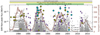 |
Fig. 1. Datasets used in this study. Grey dots indicate SXR flares of ≥M1 class registered between September 1975 and June 2017. Purple squares, olive diamonds, and cyan pentagrams denote flares associated with SEP events with fluences of f100 > 0, f800 > 103, and 105 cm−2, respectively. The brown line shows the smoothed international sunspot number (version 2). The horizontal bars on the top indicate the coverage of SXR, f10 – f100, and f800 SEP data. |
3. Methods
The relationship between solar flares and SPEs is often studied using correlation analyses (e.g. Belov 2000; Papaioannou et al. 2016) which do not, however, capture the causalities. A probabilistic approach provides a closer view of the flare-to-SPE association by considering that their relationship is not one-to-one (e.g. Dierckxsens et al. 2015; Belov et al. 2010). Here, we specifically focus on the conditional probability of an SPE being produced by a solar flare, explicitly considering that not all flares lead to SPEs.
3.1. Probabilistic approach: Observed data
First, we introduce the cumulative conditional probability (CCP) P(fi|I) of an SPE with the fluence of SEPs [cm−2] with energy above Ei (10, 30, 60, 100 or 800 MeV) exceeding the given value, fi, considering that a flare associated with the SPE had the SXR peak intensity exceeding the given value I. For example, P(f30 > 103|X1) corresponds to the probability of an SPE with the fluence f30 > 103 cm−2 being caused by a solar flare of class > X1. This probability can be calculated as the ratio of the number of flares with the SXR peak flux > I accompanied by SPEs with fluence f > fi, i.e. Nf∧I, to the total number of flares with the SXR peak flux exceeding I, i.e. NI:  . The statistical uncertainty of the probability values σP(fi|I) can be assessed as
  . To determine the number of SPEs associated with flares, Nf∧I, we used two datasets, as described in Section A.2: GOES data from 1984 – 2013 for f10 – f100 (Papaioannou et al. 2016), and from 1975 – 2017 for f800 (GLEs – Belov et al. 2010; Papaioannou et al. 2016).
Figure 2 depicts the CCP P(fi|I) as a function of the SXR peak flux for different SPE thresholds. As seen, the probability of an SPE detection increases with the SXR peak flux intensity and asymptotically approaches unity for extreme flares (> X100) for low-energy SEP events. This implies that nearly every extreme flare is expected to be accompanied by at least a soft (low-energy) SPE. However, the probability of an SPE decreases significantly with SEP energy for a given SXR peak flux value. For example, for a > X1 solar flare, the probability of detecting an SPE with the fluence f30 > 0 and f800 > 103 cm−2 is ∼20% and ∼5%, respectively. For a > X10-class flare, these probabilities are ∼80% and ∼30%, respectively.
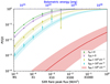 |
Fig. 2. Cumulative conditional probability P(fi|I) of SPE occurring in relation to solar flare. Different SPE thresholds are indicated by different colours, as specified in the legend. The SPE statistic (coloured symbols) is collected in nine logarithmic bins of the SXR peak flux, I, from the M1 class to the X32 class. The error bars represent one standard deviation. Coloured lines denote lognormal CDF fits with their uncertainties. The extrapolated probability of P(f800 > 108|I) roughly corresponding to the ESPE of 993/4 CE is shown in red along with its 68% credible interval (CrI; see Sect. 3.2). The bolometric energy (top abscissa) is estimated from the SXR peak fluxes using Equation S1. |
3.2. Application to an ESPE
We performed an empirical ad hoc parametrisation of the CCPs, requiring the fitting function to fit the data statistically and asymptotically approach unity with the rise of SXR peak flux. Then, the corresponding function, F(I), describing P(fi|I) should be a cumulative distribution function (CDF). The methodology of parametrisation is described in Appendix B. We found that the best fit is achieved with a log-normal distribution (Equation B.1). Next, we extrapolated the parameters of the obtained log-normal distribution to extreme events’ values, as discussed in AppendixC. The resulting CCP corresponding to an ESPE with f800 > 108 cm−2 is shown in Figure 2 in red, with the 1σ credible interval shown as a shaded area. Figure D.1 also shows the CCP for SPEs as a function of the event strength quantified in the f800 fluence for different classes of solar flares. As seen, the effectiveness of solar flares in producing SPEs increases with the flare intensity and decreases with the SPE strength. The probability of an ESPE occurring is low (≤1%) even for an extreme solar flare of X1000 class (I = 0.1 W/m2, Ebol ≈ 4 ⋅ 1033 erg), for which the probability of observing a strong GLE (f800 ≥ 105 cm−2) is close to unity. This implies that, in the framework of the applied model, only a small fraction of superflares can be accompanied by ESPEs. It is important to note, however, that while the CCP P(f800|I) is much smaller for strong but not extreme flares ≤X100, it is still non-zero. For example, the probability of an > X10 flare producing an ESPE is about 10−4. As shown in the subsequent section, this may define the relation between flares and ESPEs.
4. Occurrence rates of SPEs and ESPEs in relation to flares and superflares
From SXR observations, we can estimate the cumulative occurrence rate of flares with I > Ij per year, further denoted as νs(Ij). Then, the cumulative occurrence rate, per year, of an SEP event with a fluence > fi, associated with a flare of SXR peak intensity > Ij, can be computed as a product of the CCP and the cumulative occurrence rate:
 (1)
(1)
Since the statistics of observed solar flares do not cover the superflare range, we needed to extrapolate it using a functional form. For νs(Ij), we considered two extrapolating functional forms as proposed by Sakurai (2023), with adjustment for the SXR rescaling (factor of 1.43), as shown in Figure A.1. One is the Weibull approximation implying a roll-off at high values of SXR peak intensity, while the other, a power law, extends to higher energies, which is consistent with the recently revised statistic of superflares on sun-like stars Vasilyev et al. (2024).
We note that the two factors in Equation (1) behave differently: the CCP P(fi|Ij) increases with the value of I but saturates when approaching unity (Figure 2), while the flare’s cumulative occurrence rate νs(I) keeps decreasing (Figure A.1). This leads to a ⋂-shaped dependence of the SPE cumulative occurrence rate, ν, on I, as shown in Figure D.2 with a broad and flat top. While for weak SPEs (f800 > 104 cm−2) the highest values of ν (roughly once per 1–2 years) appear in the M1–X3 range of Ij, the top appears lower (one SPE in 10–30 year) and moves slightly towards higher Ij values (X1 – X10) for strong SPEs with f800 > 106 cm−2. For ESPEs with f800 > 108 cm−2, the top of the ν distribution yields one event in 1–30 millennia and corresponds to strong-to-moderate flares of around X1 class. This counterintuitive result occurs because of the overcompensation of the increase in CCP by the decreasing trend in the flare occurrence rate. The high-intensity tails of ν for I > X10 are greatly different for the power-law and Weibull parametrisations, but this is not important since the bulk of the SPE occurrence rate is defined by flares below the X10 class. Using spectral forms for νs(Ij) with a steeper high-intensity roll-off does not affect the results.
Figure 3 shows the SPE cumulative occurrence rate, ν (Equation 1), as a function of f800 for different thresholds of the flare intensity, Ij, ranging from M1 – X1000, as indicated by the colour code, for both power-law and Weibull parametrisations. For comparison, we also plot the f800 cumulative occurrence rate based on the neutron-monitor data for the period 1956 – 2020 (black dots – Koldobskiy et al. 2021) as well as for ESPEs listed in Koldobskiy et al. (2023, blue open dots –). The plotted ESPE occurrence rates can serve as a lower bound since more ESPEs can be potentially found over the past few millennia (Usoskin et al. 2023a; Heaton et al. 2024). As seen, superflares (grey-coloured > X1000 curves) alone cannot explain the ESPEs occurrence, nor can extreme flares of > X100. Moderately strong flares of > X10 (brown coloured curves) are needed to reproduce the ESPE rate. This implies that ESPEs are mostly produced, in the framework of the applied methodology, by ‘ordinary’ strong flares of about X10 class, which have a low probability of leading to an ESPE, but a sufficiently high occurrence rate. This implication is even stronger for the Weibull approximation of the flare occurrence rate (shown with dotted lines).
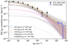 |
Fig. 3. SPE f800 fluence cumulative occurrence rate. Flares with the peak SXR flux exceeding the given GOES class are shown with different colours. Black and open blue dots represent statistics of the observed GLEs and ESPEs, respectively. Coloured dashed and dotted lines correspond to S23 power-law and Weibull approximations, respectively (see Figure A.1), and the CCP shown in Figure D.1. Shaded areas represent a 1σ uncertainty. |
5. Discussion and conclusions
We analysed the CCP of SPEs in relation to solar flares, P(fi|I), and made its probabilistic projection to extreme events. The probability first increases with the flare intensity, but then reaches saturation and approaches unity for superflares. In combination with the decreasing occurrence rate of solar flares as a function of their intensity, this leads to a counterintuitive result that strong and extreme SPEs do not require extreme flares or superflares to cause them. We suggest that the most productive ones for such (E)SPEs are strong flares of an X1 – X10 class. This can be understood in the framework of the paradigm that strong SPEs are produced not (only) by magnetic reconnection during a ‘parent flare’ in the solar atmosphere, but largely by a CME or a sequence of CMEs in the corona and interplanetary space (e.g. Gopalswamy et al. 2018). While the probability of an ESPE being related to a moderately strong flare is low, the relatively high occurrence rate of such flares versus that for superflares makes them a more likely source of ESPEs. An assumption of an intuitively expected roll-off in the occurrence rate of superflares would make this conclusion event stronger. This appears quite robust against the type of parametrisation used: ℱ for the CCP P(fi|I) (see AppendixC) and power-law versus Weibull for the flare occurrence rate, νs. This can be seen as the fact that the strongest GLEs and most intense flares are not related one-to-one (e.g. Waterfall et al. 2023). The strength and energy of an SPE is defined by many ambient factors not directly related to the ‘parent’ flare, such as the existence and parameters of a CME (or a series of them), the proximity to the heliospheric current sheet, and so on (e.g. Kong et al. 2019; Waterfall et al. 2022). Relative geometry of the Sun-Earth system is also important (e.g. Gopalswamy et al. 2012), as are the conditions of the energetic particles transport in the inner heliosphere; for example, the so-called streaming limit, which locally reduces the efficiency of acceleration (Lario et al. 2008; Reames 2017). All these factors can be favourable, or not, leading to a broad scatter of the SPE strength against the parent flare intensity (see Tsurutani et al. 2024). One can speculate that all these factors need to be favourable for an ESPE to occur. Since the flare itself does not drive these factors, there is only small random chance of ESPE occurrence, which can only be reached over a large number of events.
Of particular interest is the case of the Carrington flare of 1 Sep 1859, which was the first discovered and likely the strongest known solar flare. The flare intensity was estimated by Hayakawa et al. (2023) as ≈X80 or ≈5.77⋅1032 erg of bolometric energy. In the framework of our approach, it yields an ≈0.1% probability of an ESPE occurring (see Figure 2). This is fully consistent with the fact that, despite numerous attempts, no signal was found in cosmogenic isotopes for the Carrington event, implying that it was not accompanied by an ESPE (Usoskin & Kovaltsov 2012; Miyake et al. 2023; Uusitalo et al. 2024).
It is interesting that ESPEs tend to occur during periods of moderate or weak solar activity and not during grand activity maxima (Cliver et al. 2022; Usoskin 2023). We illustrate it in Figure 4, which depicts the relation between ESPEs and the decadal-averaged sunspot number ⟨SN⟩ over the Holocene. As seen, there is a notable correlation between the ESPE strength and ⟨SN⟩ (the slope is 0.73 ± 0.44, p-value 0.05 – estimated by MC), but it is limited to the moderate activity level. While strong ESPEs appear at the moderate activity level of ⟨SN⟩ = 50–75, weaker ESPEs can appear when ⟨SN⟩ is about 30, but none of the eight known ESPEs and candidates took place during high-activity episodes (with ⟨SN⟩> 75 or Grand minima of solar activity with ⟨SN⟩< 20). Thus, all known ESPEs and candidates correspond to the lower activity episodes, below the median value of ⟨SN⟩ = 74.5.
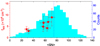 |
Fig. 4. Relation between ESPE fluence f800 (red stars, LHS ordinate) and decadal sunspot numbers ⟨SN⟩ (blue histogram – Wu et al. 2018) over the Holocene. The stars’ horizontal positions correspond to ⟨SN⟩ averaged for the preceding and subsequent decades around the decade when the ESPE occurred. The vertical blue dashed line denotes the median value ⟨SN⟩ = 74.5. |
Since the methodology used here includes ad hoc parametrisation and extrapolation of empirical relations, the uncertainties of the quantitative estimates are large. However, the result appears qualitatively robust against exact functional forms of the parametrised relationships.
Our final conclusions are listed below.
-
Extreme solar particle events are not directly related to superflares (> X300 of the SXR class or > 1033 erg of bolometric energy), but are expected to be produced by ‘normal’ strong flares of X1 – X10 class when the other coronal and interplanetary factors accidentally become favourable.
-
ESPEs tend to occur during the times of weak-to-moderate solar activity and have not been found for periods of high solar activity (grand maxima) or grand minima.
-
The apparent discrepancy between the occurrence rates of ESPEs and superflares is not outstanding and can naturally be explained by the lack of relation between these types of phenomena.
-
The conditional probability of an SPE occurring given the SXR flare is well described by a log-normal CDF for a wide range of SPE and SXR intensities.
Acknowledgments
This work was partly supported by the Research Council of Finland (projects 330063 QUASARE and 354280 GERACLIS) and EU HE project No 101135044 SPEARHEAD. VV acknowledges support from the Max Planck Society under the grant “PLATO Science” and from the German Aerospace Center under “PLATO Data Center” grant 50OO1501. AIS acknowledges support from the European Research Council (ERC) under the European Union’s Horizon 2020 research and innovation program (grant No. 101118581–project REVEAL). The ISSI Teams #510 (SEESUP, led by F. Miyake and I. Usoskin) and #23-585 (REASSESS, led by A. Mishev) are acknowledged for stimulating discussions. Data analysis was performed using NumPy (Harris et al. 2020), SciPy (Virtanen et al. 2020), pandas (The pandas development team 2020), lmfit (Newville et al. 2023), emcee (Foreman-Mackey et al. 2013), corner (Foreman-Mackey 2016) and matplotlib (Hunter 2007) open-source Python packages.
References
- Akaike, H. 1974, IEEE Trans. Automat. Contr., 19, 716 [Google Scholar]
- Aschwanden, M. J., & Güdel, M. 2021, ApJ, 910, 41 [NASA ADS] [CrossRef] [Google Scholar]
- Aschwanden, M. J., & Schrijver, C. J. 2025, ApJ, 987, 140 [Google Scholar]
- Aschwanden, M. J., Crosby, N. B., Dimitropoulou, M., et al. 2016, Space Sci. Rev., 198, 47 [Google Scholar]
- Belov, A. 2000, Space Sci. Rev., 93, 79 [NASA ADS] [CrossRef] [Google Scholar]
- Belov, A., Garcia, H., Kurt, V., Mavromichalaki, H., & Gerontidou, M. 2005, Sol. Phys., 229, 135 [NASA ADS] [CrossRef] [Google Scholar]
- Belov, A. V., Eroshenko, E. A., Kryakunova, O. N., Kurt, V. G., & Yanke, V. G. 2010, Geomagn. Aeron., 50, 21 [Google Scholar]
- Brehm, N., Bayliss, A., Christl, M., et al. 2021, Nat. Geosci., 14, 10 [Google Scholar]
- Cliver, E. W. 2006, ApJ, 639, 1206 [NASA ADS] [CrossRef] [Google Scholar]
- Cliver, E. W. 2016, ApJ, 832, 128 [Google Scholar]
- Cliver, E. W., Kahler, S. W., Shea, M. A., & Smart, D. F. 1982, ApJ, 260, 362 [Google Scholar]
- Cliver, E. W., Schrijver, C. J., Shibata, K., & Usoskin, I. G. 2022, Liv. Rev. Sol. Phys., 19, 2 [NASA ADS] [CrossRef] [Google Scholar]
- Crosby, N. B., Aschwanden, M. J., & Dennis, B. R. 1993, Sol. Phys., 143, 275 [NASA ADS] [CrossRef] [Google Scholar]
- Dierckxsens, M., Tziotziou, K., Dalla, S., et al. 2015, Sol. Phys., 290, 841 [CrossRef] [Google Scholar]
- Foreman-Mackey, D. 2016, J. Open Source Softw., 1, 24 [Google Scholar]
- Foreman-Mackey, D., Hogg, D. W., Lang, D., & Goodman, J. 2013, PASP, 125, 306 [Google Scholar]
- Gerontidou, M., Mavromichalaki, H., Belov, A., & Kurt, V. 2009, Adv. Space Res., 43, 687 [Google Scholar]
- Gopalswamy, N. 2018, in Extrem. Events Geosp., ed. N. Buzulukova, 37 [Google Scholar]
- Gopalswamy, N., Xie, H., Yashiro, S., et al. 2012, Space Sci. Rev., 171, 23 [NASA ADS] [CrossRef] [Google Scholar]
- Harris, C. R., Millman, K. J., van der Walt, S. J., et al. 2020, Nature, 585, 357 [NASA ADS] [CrossRef] [Google Scholar]
- Hayakawa, H., Bechet, S., Clette, F., et al. 2023, ApJ, 954, L3 [Google Scholar]
- Heaton, T. J., Bard, E., Bayliss, A., et al. 2024, Nature, 633, 306 [Google Scholar]
- Hudson, H., Cliver, E., White, S., et al. 2024, Sol. Phys., 299, 39 [NASA ADS] [CrossRef] [Google Scholar]
- Hunter, J. D. 2007, Comput. Sci. Eng., 9, 90 [NASA ADS] [CrossRef] [Google Scholar]
- Kahler, S. W., White, S. M., & Ling, A. G. 2017, J. Space Weather Space Clim., 7, A27 [Google Scholar]
- Koldobskiy, S., Raukunen, O., Vainio, R., Kovaltsov, G. A., & Usoskin, I. 2021, A&A, 647, A132 [CrossRef] [EDP Sciences] [Google Scholar]
- Koldobskiy, S., Mekhaldi, F., Kovaltsov, G., & Usoskin, I. 2023, J. Geophys. Res. Space Phys., 128, e2022JA031186 [Google Scholar]
- Kong, X., Guo, F., Chen, Y., & Giacalone, J. 2019, ApJ, 883, 49 [NASA ADS] [CrossRef] [Google Scholar]
- Kopp, G. 2021, Sol. Phys., 296, 133 [Google Scholar]
- Kretzschmar, M. 2011, A&A, 530, 1 [Google Scholar]
- Kurt, V., Belov, A., Mavromichalaki, H., & Gerontidou, M. 2004, Ann. Geophys., 22, 2255 [NASA ADS] [CrossRef] [Google Scholar]
- Lario, D., Aran, A., & Decker, R. B. 2008, Space Weather, 6, 1 [Google Scholar]
- Machol, J., Viereck, R., Peck, C., & Mothersbaugh III, J. 2022, GOES X-ray sensor (XRS) operational data, Tech. rep. [Google Scholar]
- Maehara, H., Shibayama, T., Notsu, S., et al. 2012, Nature, 485, 478 [NASA ADS] [Google Scholar]
- Mekhaldi, F., Adolphi, F., Herbst, K., & Muscheler, R. 2021, J. Geophys. Res. Space Phys., 126, e2021JA029351 [Google Scholar]
- Miyake, F., Nagaya, K., Masuda, K., & Nakamura, T. 2012, Nature, 486, 240 [NASA ADS] [CrossRef] [Google Scholar]
- Miyake, F., Usoskin, I., & Poluianov, S. 2019, in Extreme Solar Particle Storms, eds. F. Miyake, I. Usoskin, & S. Poluianov (IOP Publishing) [Google Scholar]
- Miyake, F., Hakozaki, M., Hayakawa, H., Nakano, N., & Wacker, L. 2023, J. Space Weather Space Clim., 13, 31 [Google Scholar]
- Newville, M., Otten, R., Nelson, A., et al. 2023, https://doi.org/10.5281/zenodo.8145703 [Google Scholar]
- Okamoto, S., Notsu, Y., Maehara, H., et al. 2021, ApJ, 906, 72 [NASA ADS] [CrossRef] [Google Scholar]
- Paassilta, M., Raukunen, O., Vainio, R., et al. 2017, J. Space Weather Space Clim., 7, A14 [NASA ADS] [CrossRef] [EDP Sciences] [Google Scholar]
- Papaioannou, A., Sandberg, I., Anastasiadis, A., et al. 2016, J. Space Weather Space Clim., 6, A42 [NASA ADS] [CrossRef] [EDP Sciences] [Google Scholar]
- Park, J., Moon, Y. J., Lee, D. H., & Youn, S. 2010, J. Geophys. Res. Space Phys., 115, A10105 [Google Scholar]
- Plutino, N., Berrilli, F., Del Moro, D., & Giovannelli, L. 2023, Adv. Space Res., 71, 2048 [Google Scholar]
- Reames, D. V. 2017, Lect. Notes Phys., 932, 55 [Google Scholar]
- Rotti, S., Aydin, B., Georgoulis, M. K., & Martens, P. C. 2022, ApJS, 262, 29 [Google Scholar]
- Sakurai, T. 2023, Physics (College. Park. Md), 5, 11 [Google Scholar]
- Schrijver, C. J., Beer, J., Baltensperger, U., et al. 2012, J. Geophys. Res. Space Phys., 117, A08103 [Google Scholar]
- The pandas development team, 2020, https://doi.org/10.5281/zenodo.3509134 [Google Scholar]
- Tsurutani, B. T., Sen, A., Hajra, R., et al. 2024, J. Geophys. Res. Space Phys., 129, e2024JA032622 [Google Scholar]
- Usoskin, I. G. 2023, Liv. Rev. Sol. Phys., 20, 2 [NASA ADS] [CrossRef] [Google Scholar]
- Usoskin, I. G., & Kovaltsov, G. A. 2012, ApJ, 757, 92 [NASA ADS] [CrossRef] [Google Scholar]
- Usoskin, I., Koldobskiy, S., Kovaltsov, G. A., et al. 2020a, A&A, 640, A17 [EDP Sciences] [Google Scholar]
- Usoskin, I. G., Koldobskiy, S. A., Kovaltsov, G. A., et al. 2020b, J. Geophys. Res. Space Phys., 125, e2020JA027921 [NASA ADS] [CrossRef] [Google Scholar]
- Usoskin, I., Miyake, F., Baroni, M., et al. 2023a, Space Sci. Rev., 219, 73 [Google Scholar]
- Usoskin, I. G., Koldobskiy, S. A., Poluianov, S. V., et al. 2023b, A&A, 670, L22 [CrossRef] [EDP Sciences] [Google Scholar]
- Uusitalo, J., Golubenko, K., Arppe, L., et al. 2024, Geophys. Res. Lett., 51, e2023GL106632 [Google Scholar]
- Vasilyev, V., Reinhold, T., Shapiro, A. I., et al. 2022, A&A, 668, A167 [NASA ADS] [CrossRef] [EDP Sciences] [Google Scholar]
- Vasilyev, V., Reinhold, T., Shapiro, A. I., et al. 2024, Science, 386, 1301 [Google Scholar]
- Verbeeck, C., Kraaikamp, E., Ryan, D. F., & Podladchikova, O. 2019, ApJ, 884, 50 [NASA ADS] [CrossRef] [Google Scholar]
- Veronig, A., Temmer, M., Hanslmeier, A., Otruba, W., & Messerotti, M. 2002, A&A, 382, 1070 [NASA ADS] [CrossRef] [EDP Sciences] [Google Scholar]
- Virtanen, P., Gommers, R., Oliphant, T. E., et al. 2020, Nat. Methods, 17, 261 [Google Scholar]
- Waterfall, C. O. G., Dalla, S., Laitinen, T., Hutchinson, A., & Marsh, M. 2022, ApJ, 934, 82 [NASA ADS] [CrossRef] [Google Scholar]
- Waterfall, C. O. G., Dalla, S., Raukunen, O., et al. 2023, Space Weather, 21, e2022SW003334 [Google Scholar]
- Wu, C. J., Usoskin, I. G., Krivova, N., et al. 2018, A&A, 615, 93 [Google Scholar]
Appendix A: Solar flare and SPE data
A.1. Solar flares in SXR
We used a catalogue of solar flares detected in SXR by the NASA/NOAA GOES (Geostationary Operational Environmental Satellite) constellation available at the National Center for Environmental Information (NCEI)2 for the period from September 1975 to June 2017. The flare intensity is often represented via its SXR (in the wavelength range 0.1 – 0.8 nm) peak flux I expressed either in units of W/m2 or so-called GOES SXR-class, defined by letter/digit combination (e.g., X1 for I = 10−4 W/m2, see Cliver et al. 2022). The peak SXR fluxes, measured before the launch of the GOES-16 instrument in 2016, were rescaled with the NOAA-recommended correction factor of ×𝒞 = 1.43 (see Verbeeck et al. 2019; Machol 2022, for details) to get the physical quantities. For the greatest SXR solar flares, we applied updated estimates of the peak flux as provided by Hudson et al. (2024). Within the considered period of time, the dataset contains 9610 flares of M class, 712 of X class, and 36 flares of X10 class and higher. We considered all flares independent of each other, even if they were produced by the same active region on the Sun.
The measured SXR peak flux of solar flares can be related to their bolometric energy via an empirical relation described by Cliver et al. (2022) based on results of statistical analyses by Schrijver et al. (2012) and Kretzschmar (2011):
 (A.1)
(A.1)
where ℱbol is expressed in ergs, I and IX1 are the SXR peak fluxes of a flare and that of the X1-class flare (IX1 = 10−4 W m−2), respectively, and 𝒞 is a scaling factor to relate the X-class to a ‘physical’ SXR peak flux value (see section 8.2.1 of Cliver et al. 2022). This is an empirical statistical relation, which may lead to case-by-case uncertainties (Cliver et al. 2022).
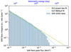 |
Fig. A.1. Solar flare SXR peak flux cumulative occurrence rate (per year). The blue histogram represents the GOES data from NOAA (1975 – 2017) – see Section A.1. Green dashed and blue dotted lines denote different extrapolations: power law (ν = 41.95 × (I/I0)−1.162 [yr−1]) and Weibull (ν = 41.95 × exp( − 10.2 ⋅ (Ik + I0k)/I0k) [yr−1], where I0 = 4.29⋅10−5 W/m2, k = 0.104), respectively, according to Sakurai (2023, – S23). |
A.2. SPE data
For the statistics of SPEs, we used several data sources.
For low-energy SPEs (from 10 to 100 MeV), we utilised a database by Papaioannou et al. (2016) which covers the period from 1984 – 2013 and is based on the GOES satellite data. The database includes information on energy-integrated fluences (expressed here in units of particles per cm2) of SEPs for energies above 10, 30, 60, and 100 MeV, further denoted as f10 through f100, respectively, as well as the association between SPEs and SXR flares.
For higher-energy SEP events (E> 800 MeV), we made use of the integral flux reconstructed by Koldobskiy et al. (2021) from analysis of ground-level enhancements (GLEs)3 registered by the ground-based network of neutron monitors (Usoskin et al. 2020a). Accordingly, we used event-integrated fluence f800 as provided by Koldobskiy et al. (2021) to characterise the strength of GLE events. The association of GLEs with their parent solar flares was mostly based on the compilation by Belov et al. (2010), covering the period 1976 – 2010, and appended with data up to GLE #71 (17 May 2012 – Papaioannou et al. 2016). Overall from 1976 through 2017, 45 GLEs (#27 – 71) were registered.
All SPEs were considered independent of each other, even if they were produced by the same active region on the Sun. Overall, the SPE dataset contains 314 events of f10 > 0 SPEs associated with flares, 122 events with f100 > 0, and 44 events with f800 > 0.
The association between GLEs and SXR flares is cross-verified between different studies (Belov et al. 2010; Papaioannou et al. 2016; Cliver 2016), especially for high-energy SPE events. Most SPEs were associated with their parent flares, making it possible to study the conditional probabilities. The fraction of SPEs, not directly associated with flares, which may be behind the solar limb, is small, from 10% for f10 to a single f800 event (a weak GLE#29 on 24-Sep-1977). Also, a small proportion, ∼10%, of SPEs were associated with SXR flares of a class below M1. Such events were excluded from the analysis, but this does not alter the results because of their small number.
Appendix B: Parameterisation of CCP of observing SPE event in relation to an SXR flare
We tested several analytical CDFs, commonly used in statistical analyses, to fit the observed CCPs for fixed fi as summarised in Table B.1.
Metrics, χ2 per degree of freedom (χ2/dof) and AIC, of the various CDF fits to the empirical CCP data (Figure 2).
The fits were obtained by minimising the standard χ2 difference between the data points shown in Figure 2 and a prescribed functional form (see Table B.1). The minimisation was performed using the Levenberg-Marquardt algorithm utilised in lmfit4 fitting package. The goodness of the fit was estimated, as illustrated in Table B.1 for SEP events with f30 > 0, f100 > 0, f800 > 3 ⋅ 103 cm−2. We also considered the Akaike information criterion (AIC, Akaike 1974), which simultaneously assesses the goodness of fit and the relative simplicity of the model to avoid overfitting. As seen, the best parameterisation, viz., systematically low values of χ2 and AIC for all fitted distributions, and particularly for strong SPEs, was obtained with the log-normal distribution:
![Mathematical equation: $$ \begin{aligned} P(f_{i}|I) = \frac{1}{2} \left[ 1+\text{ erf}\left(\frac{\ln (I)-\mu _i}{\sqrt{2}\sigma _i}\right) \right] \end{aligned} $$](/articles/aa/full_html/2025/10/aa56069-25/aa56069-25-eq11.gif) (B.1)
(B.1)
where I is expressed in W/m2, μi and σi are parameters of the fit, and erf is the error function. Similar quality and properties of the fit were also obtained for other SPE energies/intensities. We used the lognormal distribution for further analysis.
Appendix C: Extrapolation of lognormal CCP to solar extreme events
We analysed the dependence of the parameters μ and σ of the lognormal distribution (Equation B.1) on the value of f800 for strong SPEs as shown in Figure C.1. Black dots with error bars depict best fits and their 1σ confidence intervals (CIs) as obtained by applying the lmfit Python package for f800 values from 103 through 106 cm−2. As seen, both μ (panel a) and σ (panel b) increase non-linearly with f800, while being tightly linked to each other (panel c) – the Pearson linear correlation between them is 0.97. While directly measured values of f800 reach about 106 cm−2, ESPEs correspond to f800≳108 cm−2 (Koldobskiy et al. 2023), as indicated by the vertical red line in Figure C.1. Accordingly, the relationship needs to be parameterised and extrapolated via a functional form. Since μ and σ are tightly related (see Figure C.1c), we can vary only μ as a function of f800, with σ being considered as linearly related to μ. Fitting was performed by minimising the following merit function, which is an analogue of χ2:
 (C.1)
(C.1)
where n = 7 is the number of f800 fitted points, μi* = ℱ(f800, i) is the value of the fitting function ℱ for f800, i corresponding to μi, and d and e are the coefficients of a linear regression between the parameters, σ = d + e ⋅ μ. We tested several simple analytical functional forms ℱ, e.g., linear, exponential, etc., considering both the minimum value of ℛ2 and the AIC. The best fits were found for the offset power-law (denoted as ℱ1) and parabolic (ℱ2) functions, as shown in Figure C.1 and detailed in Table C.1. For ℱ2, we additionally applied a constraint that the parabola is U-shaped with the minimum located at f800 < 103 cm−2, formalised as (−b/(2c) < 3).
To explore the parameter space and assess the uncertainties of the fit parameters, we used the Markov Chain Monte Carlo (MCMC) approach by applying a Python ensemble sampler emcee5. 1D and 2D posterior probability distributions, shown with the corner plot in Figure C.2 for the parameters of the parabolic function ℱ2, indicate a significant correlation between some parameters. We estimated the credible interval (CrI) as regions corresponding to the smallest area containing 68.27% of the posterior probability mass (shown with red contours on 2D plots), equivalent to the 1σ CI in a Gaussian distribution. The most probable values of the fit parameters (calculated as the median of the selected sample) are shown in Table C.1 along with their uncertainties, for both offset power-law and parabolic functional forms.
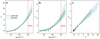 |
Fig. C.1. Extrapolation of lognormal CDF parameters μ and σ (Equation B.1) towards ESPEs. The best-fit values of μ and σ for given values of f800 and their 1σ uncertainties are shown by black points with error bars in panels a and b, while panel c shows their mutual relation. Blue and green colours correspond to the fit of μ and σ as functions of f800 performed with the MCMC approach for the offset power-law and parabolic functional forms (see Table C.1), respectively. Shaded areas correspond to 68% CrI of the fit, while the lines correspond to the median values within these CrIs. The boundary of the ESPE definition (f800 > 108 cm−2) is shown with the red vertical ESPE line. |
Parameters of the joint fitting the lognormal parameters μ and σ as a function of f800.
We used these parameter samples of the fit obtained using the MCMC ensemble sampler, for both ℱ1 and ℱ2 models, to extrapolate the functional dependencies to the ESPE case of f800 = 108 cm−2. The values of μ and σ, corresponding to ESPEs, were found to exceed ≈6 and ≈3.8, respectively. Both functional models ℱ1 and ℱ2 agree with each other within the 1σ interval, which appears confined for the ℱ2 model but somewhat wider for the ℱ1 model.
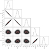 |
Fig. C.2. 1D and 2D posterior probability distributions of parabolic ℱ2 fit parameters (see Figure C.1 and Table C.1), as obtained with the MCMC sampler (see text). 1σ CrI are denoted with red contours on 2D plots. |
Appendix D: Additional figures for Section 4
Fig. D.1 shows the cumulative conditional probability of an SPE given the SXR peak flux flare, similar to Fig. 2, but as a function of f800, for flares of given cumulative class.
Fig. D.2 presents SPE cumulative occurrence rates, similar to Fig. 3, but as a function of cumulative flare peak flux.
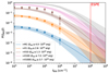 |
Fig. D.1. Cumulative conditional probability as a function of fluence and solar flare class. CCP P(f800|I) as a function of f800 for different classes of solar flares as indicated in the legend. Dots with error bars are based on the observed data (cf. Figure 2), while lines with shaded areas represent the parameteric model described in AppendixC with its uncertainties. All shown uncertainties are 1σ. |
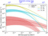 |
Fig. D.2. SPE cumulative occurrence rates as a function of flare peak flux. Cumulative occurrence rate of SPEs with the f800 fluence exceeding a given value, denoted by the colour, as a function of the intensity of the related flare. The results are shown for the two parameterisations of the flare occurrence rate (Figure A.1), viz., power-law (dashed curves) and Weibull (dotted). |
All Tables
Metrics, χ2 per degree of freedom (χ2/dof) and AIC, of the various CDF fits to the empirical CCP data (Figure 2).
Parameters of the joint fitting the lognormal parameters μ and σ as a function of f800.
All Figures
|
Fig. 1. Datasets used in this study. Grey dots indicate SXR flares of ≥M1 class registered between September 1975 and June 2017. Purple squares, olive diamonds, and cyan pentagrams denote flares associated with SEP events with fluences of f100 > 0, f800 > 103, and 105 cm−2, respectively. The brown line shows the smoothed international sunspot number (version 2). The horizontal bars on the top indicate the coverage of SXR, f10 – f100, and f800 SEP data. |
| In the text | |
|
Fig. 2. Cumulative conditional probability P(fi|I) of SPE occurring in relation to solar flare. Different SPE thresholds are indicated by different colours, as specified in the legend. The SPE statistic (coloured symbols) is collected in nine logarithmic bins of the SXR peak flux, I, from the M1 class to the X32 class. The error bars represent one standard deviation. Coloured lines denote lognormal CDF fits with their uncertainties. The extrapolated probability of P(f800 > 108|I) roughly corresponding to the ESPE of 993/4 CE is shown in red along with its 68% credible interval (CrI; see Sect. 3.2). The bolometric energy (top abscissa) is estimated from the SXR peak fluxes using Equation S1. |
| In the text | |
|
Fig. 3. SPE f800 fluence cumulative occurrence rate. Flares with the peak SXR flux exceeding the given GOES class are shown with different colours. Black and open blue dots represent statistics of the observed GLEs and ESPEs, respectively. Coloured dashed and dotted lines correspond to S23 power-law and Weibull approximations, respectively (see Figure A.1), and the CCP shown in Figure D.1. Shaded areas represent a 1σ uncertainty. |
| In the text | |
|
Fig. 4. Relation between ESPE fluence f800 (red stars, LHS ordinate) and decadal sunspot numbers ⟨SN⟩ (blue histogram – Wu et al. 2018) over the Holocene. The stars’ horizontal positions correspond to ⟨SN⟩ averaged for the preceding and subsequent decades around the decade when the ESPE occurred. The vertical blue dashed line denotes the median value ⟨SN⟩ = 74.5. |
| In the text | |
|
Fig. A.1. Solar flare SXR peak flux cumulative occurrence rate (per year). The blue histogram represents the GOES data from NOAA (1975 – 2017) – see Section A.1. Green dashed and blue dotted lines denote different extrapolations: power law (ν = 41.95 × (I/I0)−1.162 [yr−1]) and Weibull (ν = 41.95 × exp( − 10.2 ⋅ (Ik + I0k)/I0k) [yr−1], where I0 = 4.29⋅10−5 W/m2, k = 0.104), respectively, according to Sakurai (2023, – S23). |
| In the text | |
|
Fig. C.1. Extrapolation of lognormal CDF parameters μ and σ (Equation B.1) towards ESPEs. The best-fit values of μ and σ for given values of f800 and their 1σ uncertainties are shown by black points with error bars in panels a and b, while panel c shows their mutual relation. Blue and green colours correspond to the fit of μ and σ as functions of f800 performed with the MCMC approach for the offset power-law and parabolic functional forms (see Table C.1), respectively. Shaded areas correspond to 68% CrI of the fit, while the lines correspond to the median values within these CrIs. The boundary of the ESPE definition (f800 > 108 cm−2) is shown with the red vertical ESPE line. |
| In the text | |
|
Fig. C.2. 1D and 2D posterior probability distributions of parabolic ℱ2 fit parameters (see Figure C.1 and Table C.1), as obtained with the MCMC sampler (see text). 1σ CrI are denoted with red contours on 2D plots. |
| In the text | |
|
Fig. D.1. Cumulative conditional probability as a function of fluence and solar flare class. CCP P(f800|I) as a function of f800 for different classes of solar flares as indicated in the legend. Dots with error bars are based on the observed data (cf. Figure 2), while lines with shaded areas represent the parameteric model described in AppendixC with its uncertainties. All shown uncertainties are 1σ. |
| In the text | |
|
Fig. D.2. SPE cumulative occurrence rates as a function of flare peak flux. Cumulative occurrence rate of SPEs with the f800 fluence exceeding a given value, denoted by the colour, as a function of the intensity of the related flare. The results are shown for the two parameterisations of the flare occurrence rate (Figure A.1), viz., power-law (dashed curves) and Weibull (dotted). |
| In the text | |
Current usage metrics show cumulative count of Article Views (full-text article views including HTML views, PDF and ePub downloads, according to the available data) and Abstracts Views on Vision4Press platform.
Data correspond to usage on the plateform after 2015. The current usage metrics is available 48-96 hours after online publication and is updated daily on week days.
Initial download of the metrics may take a while.