| Issue |
A&A
Volume 703, November 2025
|
|
|---|---|---|
| Article Number | A109 | |
| Number of page(s) | 9 | |
| Section | Stellar structure and evolution | |
| DOI | https://doi.org/10.1051/0004-6361/202453573 | |
| Published online | 10 November 2025 | |
Unprecedentedly bright X-ray flaring in Cygnus X-1 observed by INTEGRAL
1
Dr. Karl Remeis-Observatory, Friedrich-Alexander-Universität Erlangen-Nürnberg, Sternwartstr. 7, 96049 Bamberg, Germany
2
Université Paris Cité, Université Paris-Saclay, CEA, CNRS, AIM, 91191 Gif-sur-Yvette, France
3
APC, Université Paris Cité, CNRS, CEA, Rue Alice Domont & Léonie Duquet, 75013 Paris, France
4
NASA Goddard Space Flight Center, Astrophysics Science Division, 8800 Greenbelt Road, Greenbelt, MD 20771, USA
5
CRESST and Center for Space Sciences and Technology, University of Maryland Baltimore County, 1000 Hilltop Circle, Baltimore, MD 21250, USA
6
Astrophysics Group, Cavendish Laboratory, J. J. Thomson Avenue, Cambridge CB3 0US, UK
7
Astrophysics, Department of Physics, University of Oxford, Denys Wilkinson Building, Keble Road, Oxford OX1 3RH, UK
8
University of Geneva, Department of Astronomy, Chemin d’Ecogia 16, 1290 Versoix Switzerland
9
, Washington University, MSC 1105-109-02, One Brookings Drive, St. Louis, MO 63130-4899, USA
10
European Space Agency (ESA), European Space Research and Technology Centre (ESTEC), Keplerlaan 1, 2201 AZ Noordwijk, The Netherlands
11
Julius-Maximilians-Universität Würzburg, Fakultät für Physik und Astronomie, Institut für Theoretische Physik und Astrophysik, Lehrstuhl für Astronomie, Emil-Fischer-Str 31, 97074 Würzburg, Germany
12
Departament d’Astronomia i Astrofisica, Universitat de València, C/ Dr. Moliner, 50, 46100 Burjassot, València, Spain
13
Observatori Astronòmic, Universitat de València, C/ Catedràtic José Beltrán, 46980 Paterna, València, Spain
14
Space Sciences Laboratory, 7 Gauss Way, University of California, Berkeley, CA 94720-7450, USA
15
European Space Agency (ESA), European Space Astronomy Centre (ESAC), Villafranca del Castillo, 28692 Madrid, Spain
⋆ Corresponding author.
Received:
20
December
2024
Accepted:
25
August
2025
Abstract
We study three extraordinarily bright X-ray flares originating from Cyg X-1 seen on July 10, 2023, detected with INTEGRAL. The flares had a duration on the order of only ten minutes each, and within seconds reached a 1–100 keV peak luminosity of 1.1 − 2.6 × 1038 erg s−1. The associated INTEGRAL/IBIS count rate was approximately ten times higher than usual for the hard state. To our knowledge, this is the first time that such strong flaring has been seen in Cyg X-1, despite the more than 21 years of INTEGRAL monitoring – with almost ∼20 Ms of exposure – and the similarly deep monitoring with RXTE/PCA from 1997 to 2012. The flares were seen in all three X-ray and γ-ray instruments of INTEGRAL. Radio monitoring by the AMI Large Array with observations 6 h before and 40 h after the X-ray flares did not detect a corresponding increase in radio flux. The shape of the X-ray spectrum shows only marginal change during the flares, i.e., photon index and cut-off energy are largely preserved. The overall flaring behavior points toward a sudden and brief release of energy either due to the ejection of material in an unstable jet or due to the interaction of the jet with the ambient clumpy stellar wind.
Key words: accretion, accretion disks / black hole physics / stars: black holes / stars: jets / X-rays: binaries / X-rays: individuals: Cyg-1
Deceased June, 17, 2025.
© The Authors 2025
 Open Access article, published by EDP Sciences, under the terms of the Creative Commons Attribution License (https://creativecommons.org/licenses/by/4.0), which permits unrestricted use, distribution, and reproduction in any medium, provided the original work is properly cited.
This article is published in open access under the Subscribe to Open model. This email address is being protected from spambots. You need JavaScript enabled to view it. to support open access publication.
1. Introduction
Cyg X-1 is one of the best-studied stellar-mass black hole X-ray binaries. Discovered in 1962 (Bowyer et al. 1965), the black hole has a mass of 21.2 ± 2.2 M⊙ (Miller-Jones et al. 2021) and is in an almost circular 5.6 d orbit with its donor, HDE 226868 (Bolton 1972), at a separation of 0.24 AU and a distance of  kpc from us (Miller-Jones et al. 2021). Systematic long-term X-ray monitoring began around 1975 with Ariel V (Holt et al. 1979), continued with Ginga (Kitamoto et al. 2000), CGRO/BATSE (Ling et al. 1997), and the RXTE/ASM (Grinberg et al. 2013), and is currently provided by MAXI and Swift/BAT. Cyg X-1 has also been the subject of detailed campaigns of pointed observations, with missions such as RXTE (Pottschmidt et al. 2003a; Wilms et al. 2006; Grinberg et al. 2014), INTEGRAL (e.g., Del Santo et al. 2013; Cangemi et al. 2021), and NICER (e.g., König et al. 2024). In total, almost half a century of X-ray monitoring has shed light on the variability of Cyg X-1 on timescales from milliseconds to months.
Cyg X-1 is a persistent X-ray source that, similar to other black-hole binaries (BHBs), exhibits two canonical states, characterized by distinct spectral and timing properties (e.g., Grinberg et al. 2013; König et al. 2024, and references therein). The “hard state” shows an X-ray spectrum that can mainly be explained by the Comptonization of soft seed photons by a hot electron plasma. In the “soft state”, thermal emission from the accretion disk dominates the spectrum, although some Comptonized radiation is still observed. Between the two main states, Cyg X-1 transits through the so-called “intermediate state”, with changes between different states typically occurring on timescales of days to weeks. On short timescales ranging from milliseconds to minutes, power spectra and other timing quantities show characteristic state-dependent behavior, interpreted as arising from a combination of variability in the accretion flow and in the Comptonizing plasma (König et al. 2024, and references therein). Superimposed on and potentially distinct from this variability, flares with a duration of seconds to minutes have been observed (e.g., Wilms et al. 2007). Consistent with such flaring activity, the power spectra sometimes display an additional noise component below ∼0.01 Hz (e.g., Vikhlinin et al. 1994).
Cyg X-1 has also shown variable but persistent radio emission, which is due to the presence of a radio jet (Gallo et al. 2005; Rushton et al. 2012). The radio variability has been tracked during various years-long campaigns with, for example, the Ryle telescope, the Arcminute Microkelvin Imager (AMI), or MERLIN (e.g., Fender et al. 2006; Gleissner et al. 2004; Rodriguez et al. 2015a). In addition to a correlation between radio and hard X-ray flux in both the hard and the soft state (Gleissner et al. 2004; Zdziarski et al. 2020), these campaigns also displayed the (rare) presence of radio flares, which may resemble bubble ejection events in blazars (e.g., Fender et al. 2006; Pooley 2017). This includes a case where an X-ray flare was followed by a radio flare ∼7 min later (Wilms et al. 2007).
X-ray flaring on intermittent timescales has also been observed in black-hole low-mass X-ray binaries (BH-LMXBs) during their outbursts. Worth highlighting is the rich variability of GRS 1915+105, in particular for its repeatability (Belloni 2010), while less predictable flaring was seen, for instance, in V404 Cygni (e.g., Alfonso-Garzón et al. 2018; Tetarenko et al. 2017). Flaring in the radio band is an established signature of the hard- to soft-state transition of BHB outbursts (Fender & Belloni 2004). On much shorter timescales of ≲1 s, flaring and variability have been attributed to changes in the inner disk region and magnetic reconnection events above it (Lyubarskii 1997; Uttley & Malzac 2025). Here we report on a series of exceptionally bright flares observed with INTEGRAL on July 10, 2023. During these flares, which occurred during a time interval of little more than one hour and lasted only for ∼5–10 minutes each, the X-ray emission of Cyg X-1 was brighter by a factor of more than 20 compared to the brightest emission seen in the more than 20 Ms of INTEGRAL observations taken since its launch in 2002. In Sect. 2 we present the light curves of the flares. We then put the time of the flares in context of the long-term spectral and state evolution of Cyg X-1 in Sect. 3 and discuss the detailed behavior of the source in Sect. 4. We discuss and summarize our results in Sect. 5.
2. Strong flaring of Cyg X-1
Cyg X-1 has been a regular target of INTEGRAL since its launch in 2002 (e.g., Pottschmidt et al. 2003b; Del Santo et al. 2003; Cadolle Bel et al. 2006). Since 2013, our team has organized regular monitoring observations during the two observing windows each year, given by visibility constraints, with the aim to further constrain the hard X-ray polarization found with INTEGRAL (Laurent et al. 2011; Jourdain et al. 2012; Rodriguez et al. 2015a). As part of these regular observations, on July 10, 2023, during INTEGRAL’s revolution 2661, strong flaring was detected through the MMODA interface (Neronov et al. 2021; Ferrigno et al. 2022)1, within a time interval of < 1 h long, with a flux that greatly exceeded those detected since the launch of INTEGRAL.
For a detailed analysis, we extracted spectra and light curves from all the IBIS/ISGRI (Ubertini et al. 2003; Lebrun et al. 2003) and JEM-X (Lund et al. 2003) data of Cyg X-1 taken during revolution 2661 using the offline science analysis (OSA) software package 11.2. The flares were confirmed in two INTEGRAL Science Windows, i.e., slightly offset pointings of the INTEGRAL satellite2. Since the two Science Windows have off-axis angles of  and
and  , respectively, placing Cyg X-1 barely at the edge of the field of view of JEM-X, no spectral analysis with JEM-X is possible. The minute-scale evolution of the flares is shown in Fig. 1. The IBIS and JEM-X light curves clearly show the flaring behavior (Fig. 1a), as does the total event rate measured in the spectrometer on INTEGRAL (SPI: Vedrenne et al. 2003, see Fig. 1c). No simultaneous information is available in the optical, since Cyg X-1 was outside the ∼5° field of view of INTEGRAL’s optical monitor.
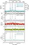 |
Fig. 1. Variability of Cyg X-1 on July 10, 2023. (a) IBIS and JEM-X light curves of the flares during rev. 2661. Gray bands indicate the time ranges of the flares. (b) Variation of the hardness ratio, HR = (H − S)/(H + S), between the 30–60 keV and 60–120 keV IBIS light curves. (c) Evolution of the total event rate in the SPI detector, dominated by Cyg X-1. (d) and (e) IBIS light curves for the two other sources, Cyg X-3 and 3A 1954+319, which are unaffected by the flare of Cyg X-1 in the field of view. Lighter colors indicate the 30–60 keV rate, and the darker ones indicate the 60–120 keV rate. (f) Count rates in those pixels of IBIS illuminated and non-illuminated by Cyg X-1. The changes in the base count rate around MJD 60135.27, MJD 60135.31, and MJD 60135.35 are due to the repointing of INTEGRAL, resulting in a change in the number of (non-)illuminated pixels and of the vignetting of the source. |
In Fig. 2, we compare the count rate measured in 60 s bins during the flares to the distribution of the count rates measured in the other ∼330 000 60 s bins covering the ∼23 yr of Cyg X-1 INTEGRAL monitoring (a total exposure time of ∼20 Ms). The flares clearly represent the brightest events ever seen for Cyg X-1 with INTEGRAL.
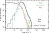 |
Fig. 2. Distribution of count rates in 60 s bins for all IBIS observations of Cyg X-1, separated by state as determined following Grinberg et al. (2013). The bin width of the rate histogram is 80 cts s−1. The count rates reached by the flares discussed in this paper are indicated within the bracket. At no time before the flares have rates of 350 cts s−1 or higher been reached. Therefore, the flares by far represent the brightest observations ever seen with IBIS for Cyg X-1. |
The exceptional brightness of Cyg X-1 during the flares makes it important to rule out the possibility that they originate from other events in the field of view, such as a background flare or a gamma-ray burst. First, we checked other sources in the same field for signs of flaring. The light curves of Cyg X-3 and 3A 1954+319, the most significantly detected sources in the field of Cyg X-1, display only a minuscule flux increase during the flaring period (Figs. 1d and e). This slight increase is likely due to effects of the deconvolution algorithm in the OSA, where a small fraction of the flux of other sources in the field of view can be misattributed to the source under study (Goldwurm et al. 2003).
In addition, we generated the light curve of Cyg X-1 without relying on deconvolution. Since IBIS utilizes a coded mask, each source in the field of view, for a given pointing direction, only illuminates a subset of pixels. Figure 1f shows the count rate measured in those pixels of IBIS that are illuminated by Cyg X-1 (Pixel Illumination Fraction, PIF > 0.7) and compares it with those that are not illuminated. The only clear signal originates from Cyg X-1 itself. No increase is seen in the pixels that are not illuminated by Cyg X-1. This clearly illustrates that the flares are not caused by any background activity. Since the likelihood that the flares arise from a serendipitous source very close to Cyg X-1 is extremely small, we conclude that the flares must come from Cyg X-1 itself.
Finally, while no pointed observations with instruments on other spacecraft were performed during the flares, Cyg X-1 was also monitored with MAXI, which provides on-demand light curves in user-defined energy bands3. These light curves are shown alongside the longer-term behavior around the flare in Fig. 3. A slight increase in count rate at the time of the flares is apparent (Fig. 3d) and might be attributable to the flare (partially) occurring during a MAXI exposure, which are generally separated by one orbit of about 90 min. We therefore conclude that the flares are indeed intrinsic to Cyg X-1.
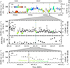 |
Fig. 3. Long-term IBIS and BAT light curve of Cyg X-1. The top panel shows the source behavior in a broader context, while the lower panels focus on the days surrounding the flare. (a) Swift/BAT (gray) and IBIS count rates, colored by the photon index of the corresponding Science Window, determined by applying the bknpower model. The canonical state of Cyg X-1 derived from the MAXI light curves according to Grinberg et al. (2014) is shown in the color strip at the top edge of the panel. The time of the flaring episode is indicated by the vertical dotted teal line. (b) IBIS data: same as that shown in (a), but focusing on a shorter time interval and including the MAXI rates instead of the Swift/BAT rates. (c) The radio flux density measured with AMI. (d) MAXI on-demand data (gray), together with the IBIS data colored as above). The interval between start of the first and end of the third flare is shaded in light gray and the length of each pointing is indicated by the horizontal error bars. A slight increase in the MAXI flux is visible around the time of the flare. |
3. The flaring episode in context
We now examine the behavior of Cyg X-1 in the months surrounding the flaring episode. As shown in Fig. 3a, the flares occurred during a phase when the hard flux of Cyg X-1 rose. Such a behavior is commonly observed in this source during transitions from the soft state to the hard state. Indeed, the well-established classification by Grinberg et al. (2013), based on MAXI monitoring and illustrated in Fig. 4, places Cyg X-1 close to the soft-to-intermediate-state transition during the flare. In the subsequent four daily scans, Cyg X-1 briefly entered the intermediate state.
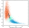 |
Fig. 4. Hardness–intensity diagram of Cyg X-1 determined from MAXI data. The position of Cyg X-1 during the flare is indicated by the black star. Red, green, and blue dots indicate individual bins in the daily light curves of MAXI, classified as soft, intermediate or hard state, respectively (Grinberg et al. 2013). The source behavior four days before and four days after the flaring episode is indicated by arrows pointing toward later observations and becoming lighter with increased separation from the flare. |
The general source behavior in the time surrounding the flaring episode was typical for Cyg X-1. Reviewing the INTEGRAL spectroscopy over the days surrounding the flare, no strong or sudden changes in the hard photon index are apparent, implying a stable geometry of the Comptonizing plasma without any sudden change in flux or hardness (Fig. 3b).
Some black hole X-ray binaries show increased radio flaring during such state transitions. To investigate the possibility of a correlated radio flare, we used data from AMI (AMI Consortiu et al. 2008). This 15 GHz radio monitoring instrument consists of two 10 minutes pointings for each day with appropriate observing conditions, separated by a calibration observation. The radio flux density per 10 min pointing and for one linear polarization direction, i.e., Stokes I + Q, are shown in Fig. 3c. AMI provided snapshots shortly before the flaring episode at MJD 60135.0225 (6.4 h before the first flare) and then 40.4 h after the last flare at MJD 60137.0145, showing that the flux increased from 7.7 mJy to 16.5 mJy, which is within the range of typical variability in the soft to soft-intermediate state (Rodriguez et al. 2015a; Lubiński et al. 2020). Over the following five days, the radio flux density continuously decreased. The ∼2 d data gap starting just before the flares prevents us from making any statement about the presence of a simultaneous radio flare.
4. Source behavior during the flares
Figure 5 shows a zoom-in on the IBIS light curves at 5 s resolution. The first and third flares are characterized by very fast rises lasting 30–50 s, with very fast doubling timescales of 15 s. These are followed by a “flat top” phase with an average IBIS count rate of ∼500 cts s−1, but with very strong normalized rms variability on timescales of tens of seconds – 51% and 36% for flare 1 and 3, respectively, at a time resolution of Δt = 10 s, and slightly less at 20 s. This variability is significantly increased compared to the 24% at Δt = 10 s measured outside the flares4. At the end of the flares, Cyg X-1 quickly returns to its previous count rate, and the variability returns to its pre-flare value.
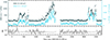 |
Fig. 5. Top: JEM-X and IBIS light curves of the three flares in the 3–10 keV and 30–60 keV band with a 10 s and 5 s time resolution, respectively. The y-axis for the IBIS data is shifted up for readability. Bottom: Hardness ratio light curve with a time resolution of 60 s. The hardness ratio is defined as HR = (H − S)/(H + S) for 30–60 keV and 60–120 keV. The gap starting around 1900 s is due to a repointing of INTEGRAL. |
In contrast, the second flare is characterized by a sudden increase in normalized rms variability (39% at Δt = 10 s) and a much slower rise (doubling time scale: ∼150 s) to a peak count rate of about 1400 cts s−1. Unfortunately, the decay back to the pre-flare luminosity is only partially covered due to a spacecraft slew, but overall, the shape of the second flare appears to be almost triangular or Gaussian in shape. The rms variability during this episode is again higher at 36% than outside of the event.
As discussed in Sect. 3, at timescales of hours to years, flux changes in Cyg X-1 are closely connected with spectral changes, as the source moves from the hard to the soft state and back. We illustrate this in the hardness-intensity-diagram of Cyg X-1 shown in Fig. 6, which is based on 100 s resolution data from all 22 years of INTEGRAL-monitoring of the source. In contrast, despite the large flux amplitude during the flares, the spectral hardness remains almost constant during these episodes (Fig. 6, teal data points; see also Fig. 1 for a light curve of the hardness ratio).
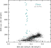 |
Fig. 6. Evolution of the hardness ratio and count rate over the course of the three outbursts in teal, compared to all other INTEGRAL observations of Cyg X-1 in gray. A bin time of 100 s was used for each data point. No clear trend toward a softening or a hardening with increasing flux is visible. |
To further quantify possible changes of the spectral shape, we extracted IBIS spectra from each flare as well as a spectrum for the time outside the flares (defined as the time interval outside the shaded regions in Fig. 1). Due to the off-axis angle of > 5° during the flare, we did not use the JEM-X data for spectral analysis. To take into account calibration uncertainties, a systematic uncertainty of 3% of the count rate was added in quadrature to the statistical uncertainty of each spectral bin.
We modeled the four spectra using typical X-ray spectral models for black hole X-ray binaries in the hard X-ray band: a simple power law, an exponential cutoff power law (cutoffpl), a broken power law (bknpow), and thermal Comptonization (comptt; Titarchuk 1994). The latter three are all able to describe a break or cutoff in the power law spectrum. The best fitting parameters are listed in Table 1. All uncertainties are given at the 90% level for one parameter of interest, and we employed ISIS5 for spectral fitting. The simple power law is unable to provide a satisfactory fit, leading to χ2/d.o.f. of 88.0/60, 145.7/60, and 120.3/60 for the three flares, respectively. The three models with an intrinsic turnover or break, those shown in Fig. 7, all describe the spectra well. This is in agreement with previous studies, which have shown that the break in the bknpow model describes the spectra of BHBs comparably well to the cutoff power law and even more complex jet models (Markoff et al. 2003; Nowak et al. 2011).
Best-fit parameters for the IBIS spectra of the time outside of the flares and the three flares.
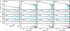 |
Fig. 7. IBIS spectra for revolution 2661 with the three flaring intervals removed (“no flare”) and for the three flares. Top: Unfolded spectra and the best-fit cutoffpl continuum. Middle: Residuals between the data and the best-fit models of Table 1. Bottom: Ratio between each flare spectrum and the no flare spectrum. |
A direct comparison between the non-flare and flare spectra, determined by dividing one by the other, shows that the flare spectra are slightly softer (Fig. 7, bottom panel). In the cutoffpl-fits this softening is reflected by a decrease in the folding energy. Similarly, the comptt models describe the softening as a decrease in the temperature of the Comptonizing plasma, kTe, together with a strong increase in the optical depth (see Table 1). We caution, however, that the data are not good enough to distinguish between these different models, and that the energy coverage of IBIS alone is not sufficient to separate the spectral continuum from the relativistic reflection hump that contributes significantly in the IBIS-band. A direct physical interpretation of the spectral parameters is therefore unadvisable.
Using the comptt model, the peak 1–100 keV luminosities are 1.1 × 1038 erg s−1, 2.6 × 1038 erg s−1, and 2.2 × 1038 erg s−1, for flare 1 through 3, while the total 1–100 keV fluence contained in the three flares is 3.01 × 1040 erg, 4.74 × 1040 erg, and 3.84 × 1040 erg. As these luminosities rely on the extrapolation of the spectral fits toward lower energies, they are only a rough lower limit. Even though we do not have direct spectral data, we nevertheless can infer from the JEM-X that the soft emission likely shows an increase similar to that in the luminosities in the 30–100 keV range, which are 2.3 × 1037 erg s−1, 4.3 × 1037 erg s−1, and 3.5 × 1037 erg s−1, for the three flares, respectively.
The hard photon index Γ1 ∼ 2.1−−2.4, inferred from the brokenpl fits during the three flares and the surrounding observation, matches what has been observed in Cyg X-1 during the soft to intermediate state (e.g., Nowak et al. 2011; Lubiński et al. 2020). It is remarkable that the spectra during the flares, especially flare 1 and flare 3, show very little change in spectral slope. Only the spectra of flare 2 display mild softening. This becomes visible through the ratio with the non-flare spectrum, which decreases toward higher energies, as seen in Fig. 7. This contrasts with the rather vertical evolution in the hardness-intensity diagram of Fig. 6 but might result from the selected energy bands and time binning.
5. Discussion and conclusions
Before we discuss the possible physical origin of the flares, we briefly summarize their main properties:
-
The three flares represent extreme source behavior not previously observed in the 21 years of monitoring of Cyg X-1 with INTEGRAL, nor in the earlier RXTE monitoring between 1997 and 2012.
-
The flares occurred during the soft-intermediate state, when Cyg X-1 was moving toward the hard state.
-
The flares occurred at orbital phase, ϕorb = 0.01, based on the ephemeris of Brocksopp et al. (1999), i.e., close to upper conjunction of the black hole.
-
The flares have peak luminosities in the 1–100 keV band ranging from 1.1 − 2.6 × 1038 erg s−1 (4.1 − 9.7% LEdd), exhibit a dynamic flux range of ∼15, and last about 400 s each, with fluences of 3 − 5 × 1040 erg each.
-
The intensity profiles are complex, with fast rise and decay times of ∼10 s for the first and third flare, and a slow rise and fast decay for the second flare.
-
During all three flares, the normalized rms variability is significantly increased.
-
There is little spectral change in the hard X-rays, with only a slight softening > 30 keV (see ratio panel in Fig. 7).
Besides their timing properties mentioned above, it is the extreme peak luminosities that make the flares stand out above the typical variability seen in Cyg X-1. To our knowledge, the only similar events in Cyg X-1 were detected by BATSE in 1999 April (Stern et al. 2001)6 and RXTE in 2005 April (Wilms et al. 2007). Both events had a similar duration of ∼10 min and the latter coincided with a radio flare that was delayed by about 400 s with respect to the X-ray flare. The flaring episode detected in 1999 originated from the hard state and consisted of two distinct outbursts each with a duration of ∼1 ks or 15 min. They show a similarly complex temporal evolution to the flares we observed and reached a peak luminosity of L> 30keV ∼ 6.9 × 1038 erg s−1, for the distance of 2.22 kpc. Interestingly, in the case of Stern et al. (2001) stronger and more rapid variability was seen below 100 keV compared to harder X-rays. During the flare reported by Wilms et al. (2007) Cyg X-1 was in the intermediate state, transitioning toward the hard state, similar to the flares observed by INTEGRAL. A notable difference is the lower dynamic range: while we observe an approximate 15-fold increase in hard X-ray flux, Wilms et al. (2007) reported the radio and X-ray flux increase by only about a factor of three7. Radio flares with behaviors similar to that studied by Wilms et al. (2007) were also discussed by Fender et al. (2006), including a strong 140 mJy radio flare lasting about one hour during the intermediate state of Cyg X-1. Unfortunately these radio flares lacked simultaneous X-ray data. The orbital phase aligns closely with phase zero. However, we would primarily expect the absorption to vary as a line-of-sight effect (Grinberg et al. 2015; Szostek & Zdziarski 2007), rather than being caused by phenomena related to the accretion flow itself. For comparison, the flare reported by Wilms et al. (2007) occurred around orbital phase 0.82. Concerning the spectral shape, the necessity of a cutoff favors a thermal origin of the X-ray emission, rather than synchrotron emission. Jet models such as those discussed by Markoff et al. (2005), Nowak et al. (2011), Maitra et al. (2017), Kantzas et al. (2021) can, however, produce spectral shapes more complex than a simple power law. A jet origin for the observed flares therefore cannot be excluded based on spectral shape.
Before investigating the possible origin of the flares, we emphasize that the flares discussed here differ from the shorter-term variability in accreting black holes, which is sometimes explained in terms of shot-noise (e.g., Bhargava et al. 2022; Gierliński & Zdziarski 2003). The latter is thought to be connected to magnetic reconnection and the evolution of plasmoids in a current sheet above the disk (e.g., Ripperda et al. 2020; El Mellah et al. 2022; Merloni & Fabian 2001) and occurs on timescales of 10 − 100 rg/c. The variability of ∼10 min seen here, however, corresponds to 106 rg/c, or approximately the light crossing time between the donor and the black hole8. Conversely, following a simple scaling by mass as appropriate for black holes, the minute-scale variability as seen in super-massive BHs corresponds to millisecond variability in BHBs.
Such short-term variability has also been attributed previously to the innermost region of the disk. Variable seed photons from the disk can be upscattered in the corona to induce variability in harder energy-bands (Uttley & Malzac 2025, and references therein). In such a scenario, the dynamic timescale is, however, on the order of 10−3 s comparable to the Keplerian timescale, and is therefore much faster than the observed flaring episodes (Lyubarskii 1997; Done et al. 2007). An overview of the different timescales in accreting black holes is given by Kara & García (2025). If the variability originates from the disk, it must therefore have its origin in the outer regions, where the Keplerian and viscous timescales are much longer. In such a case, the model of propagating fluctuations could be considered a possible explanation for the flares. Under this assumption, aperiodic fluctuations in the accretion are introduced, classically by turbulent changes in the disk viscosity at all radii of the disk. These fluctuations propagate inward toward the hotter region of the accretion disk, reproducing the observed time lags and power spectral density (see, e.g., Lyubarskii 1997; Uttley et al. 2014; Ingram & Done 2011). A sudden increase in the mass accretion rate originating at a radius of ∼102 rg could lead to variability on the order of 100 s, corresponding to the viscous time scale. The inward propagation is, however, a diffusion process and smoothens out the induced variability. The rapid rise and decay time of the flares are therefore atypical for propagating fluctuations. Furthermore, the model is usually only applicable to stochastic variability, not individual flares. Due to a lack of soft spectra and light curves, however, such a scenario cannot be fully ruled out.
Similarly, an explanation through the dissipation time, tD, after magnetic heating, as used by Merloni & Fabian (2001) following earlier studies by Haardt et al. (1994), requires a region size of
 (1)
(1)
with the unitless dissipation velocity, b = c/vdiss. This is much larger than the inner regions of the accretion disk. Accretion fluctuations alone are therefore disfavored as explanations, but could still serve as triggers for downstream changes in the jet or corona.
For examples of flaring on timescales of hours, we can broaden our view to include other BHB systems beyond Cyg X-1. Flaring has been observed in the radio band for several transient black hole X-ray binaries, where they occur around state transitions and may be correlated with changes in the X-ray timing behavior (e.g., Fender et al. 2009; Miller-Jones et al. 2012). This is relevant to our discussion, as these have also been attributed to ejection events through the jet. However, since these state transitions occur on timescales of days, they represent phenomena on very different timescales, and the physical mechanism behind these flares can therefore differ. Direct observations of such hour-long radio flares are rare. Homan et al. (2020) describe a strong radio flare in MAXI J1820+070, lasting for ∼2.5 h and reaching ∼50 mJy and accompanied by a quasi-simultaneous weak flare in the 7–12 keV NICER band. In this case, the X-ray flux only increased by a few percent. Flaring on a timescale of minutes in the optical and X-ray has also been studied during the 2015 outburst of V404 Cygni (Rodriguez et al. 2015a; Tetarenko et al. 2017; Alfonso-Garzón et al. 2018). Here, these flares display a similar complexity in shape to those seen in Cyg X-1, albeit at a much lower dynamic range. Explanations for the type of minute-long flares discussed here build on the observation that, for those flares where simultaneous broad-band data exist, flaring is not limited to the X-rays alone, but seen across the electromagnetic spectrum. Time delays are common, where longer wavelengths are delayed with respect to shorter ones (e.g., Fender et al. 2023, and references therein). As suggested by Fender & Belloni (2004) and Wilms et al. (2007), a possible model explaining these events involves some form of ejection event, similar to the flaring seen in blazars first discussed by van der Laan (1966). In such models, a bubble of relativistic electrons is ejected from the accretion flow and subsequently cools down, moving the peak of the emission to longer wavelengths. The slight spectral changes seen in the hard X-rays are interpreted as a change of the Compton-y-parameter due to the expansion and cooling of the ejected material. See Younsi & Wu (2015) for detailed computations of plasmoid ejections that take general relativistic effects into account and suggest that strong variability and multiple reflares on timescales of tens of rg/c are, in principle, possible. Such ejections have been proposed to explain the flares in the light curves of V404 Cygni with timescales of ∼200 s by Maitra et al. (2017) on the basis of multiwavelength data. In this case, a predominant disk origin was explicitly ruled out on the basis of correlated optical variability. The very characteristic heartbeat variability and the particularly large orbital period, and therefore disk, make V404 Cygni a unique system (Fender & Belloni 2004; Steeghs et al. 2013). This might limit the extent to which explanations for flaring in V404 Cygni can be applied to Cyg X-1, as the disk might behave very differently. Nevertheless, we maintain that the physics close to the black hole should still be similar and V404 Cygni serves as a valuable point of comparison.
As suggested by Rodriguez et al. (2015b) for V404 Cygni, the amplitude of the flaring could be increased due to directly boosted radiation when the jet axis is pointed directly toward the observer. Such a boosting would imply a fairly large deviation of the jet direction during the flares with respect to its default orientation. The nominal angle between the jet axis (and the orbital angular momentum) and our line of sight at upper conjunction (ϕorb = 0) is ∼60° (Krawczynski et al. 2022; Miller-Jones et al. 2021; Orosz et al. 2011). Such a large deviation is difficult to achieve. Models for the warping of the inner accretion disk in Cyg X-1 imply a warp of only ∼30° (Ibragimov et al. 2007) in order to explain the ∼150 d or ∼294 d superorbital variability in the system (Zdziarski et al. 2011; Brocksopp et al. 1999; Priedhorsky et al. 1983; Kemp et al. 1983) and the optical polarization variability (Kravtsov et al. 2023, and references therein). It is therefore unlikely that regular disk warping and variable boosting is the sole source of variability. An alternative explanation for the flares is the interaction of structures in the stellar wind of the high-mass donor star and the jet. Based on the numerical modeling of clump-jet interactions, Perucho & Bosch-Ramon (2012) show that for winds with a steep clump size distribution, it is possible for large clumps to enter the jet and be completely disrupted, potentially even choking off the jet. The simulations by Perucho & Bosch-Ramon and Araudo et al. (2009) predict rare, but luminous flares with durations of 1000 s (Rclump/1011 cm)(cc/108 cm), where Rclump is the clump radius and cclump = (2Ljet/πvjetρclumpRjet2)1/2 is the speed of sound in the clump. Here, vjet is the speed of the jet, Ljet its luminosity, and Rjet its radius at the point of interaction, while ρclump is the density of the clump. Observations of X-ray dips in Cyg X-1 show that the wind from its donor, HDE226868, is clumpy (Hirsch et al. 2019; Grinberg et al. 2015, and references therein). Line-of-sight variations of the absorbing column are stronger near the black hole’s upper conjunction (Grinberg et al. 2015), indicating that a greater number of clumps pass through our line of sight, probably close to the black hole. This is exactly the time interval when the flare was observed, although this is probably a coincidence. We note, however, that if the flare is caused by a clump destruction event, it is puzzling why its spectral shape would resemble that seen outside the flare, and why three flares are observed instead of just one. In addition, while clumps are normal in high-mass stellar winds (Owocki et al. 1988, and references therein), with a filling factor of ∼11% for Cyg X-1 (Rahoui et al. 2011), they are not expected to exist in low-mass X-ray binaries where flaring is also observed.
To conclude, we serendipitously observed an unprecedented set of ∼10 minute long, X-ray flares with fluences in excess of 1040 erg, and hard X-ray luminosities at least three times higher than anything seen before in approximately 22 years of INTEGRAL monitoring of Cyg X-1. The flares occurred in a state where the accretion flow of black hole binaries is hypothesized to be unstable. The strong flaring might be related to (i) some kind of ejection event, (ii) a restructuring of the outflow (“jet”) in the system, or (iii) the interaction of a clump in the stellar wind with the jet. The observations presented here illustrate the need for continued monitoring even of supposedly “well-known” sources, since it allows us to catch dramatic and very rare events in such systems.
A collection of spectra, images, and light curves of Cyg X-1 obtained with the INTEGRAL telescope is available at https://www.astro.unige.ch/astroordas/mmoda
The science windows are 266100120010 (MJD 60135.273–60135.311, live time 1611 s), and 266100130010 (MJD 60135.312–60135.351, live time 1943 s), with a brief slew between them. Here and elsewhere in the paper, all MJDs refer to the local INTEGRAL satellite time system and are not barycentered.
The normalized rms-variability is only an approximate estimator for the variability in the case of red noise light curves (Vaughan et al. 2003), but unfortunately the short duration of the flares precludes a more detailed characterization of the variability properties, for example, through power spectra.
We thank J. Poutanen and A. Zdziarski for pointing us towards this publication after submission to arXiv.
Since the PCA and IBIS energy ranges differ significantly, a more precise comparison of the fluxes is difficult. In addition, the peak X-ray flux of the RXTE flare could be underestimated as RXTE only observed its decay.
We caution that the term “flare” is not well-defined in astronomy, and may denote events on very different timescales. For black hole X-ray binaries alone, “flare” has been used for large amplitude flux changes on time scales of seconds, minutes, days, and months, which are likely to be due to very different physics. In the following, we use the term solely for flux changes on timescales less than a few 100 minutes.
Acknowledgments
We especially acknowledge the crucial contribution of Katja Pottschmidt – not only to this paper but the field of Black-hole timing in general. Without her support, mentorship, and scientific insight this work would not have been possible. Her untimely passing is felt sorely. This work has been partially funded by the Bundesministerium für Wirtschaft und Klimaschutz under Deutsches Zentrum für Luft- und Raumfahrt grant 50 OR 1909. This research is supported by the DFG research unit FOR 5195 ‘Relativistic Jets in Active Galaxies’ (project number 443220636, grant number WI 1860/20-1). TB & JR acknowledge partial funding from the French Space Agency (CNES). The material is based upon work supported by NASA under award number 80GSFC24M0006. MP acknowledges support by the Spanish Ministry of Science trough Grant PID2022-136828NB-C43, and by the Generalitat Valenciana through grant CIPROM/2022/49. The research is based on observations with INTEGRAL, an ESA project with instruments and science data center funded by ESA member states (especially the PI countries: Denmark, France, Germany, Italy, Switzerland, Spain) and with the participation of Russia and the USA. This research has made use ISIS 1.6.2-51 (Houck & Denicola 2000) and of ISIS functions (ISISscripts) provided by ECAP/Remeis observatory and MIT (https://www.sternwarte.uni-erlangen.de/isis/).
References
- Alfonso-Garzón, J., Sánchez-Fernández, C., Charles, P. A., et al. 2018, A&A, 620, A110 [NASA ADS] [CrossRef] [EDP Sciences] [Google Scholar]
- AMI Consortium, Zwart, J. T. L., Barker, R. W., et al. 2008, MNRAS, 391, 1545 [NASA ADS] [CrossRef] [Google Scholar]
- Araudo, A. T., Bosch-Ramon, V., & Romero, G. E. 2009, A&A, 503, 673 [NASA ADS] [CrossRef] [EDP Sciences] [Google Scholar]
- Belloni, T. M. 2010, in The Jet Paradigm, ed. T. Belloni (Berlin, Heidelberg: Springer), Lect. Notes Phys., 794, 53 [NASA ADS] [CrossRef] [Google Scholar]
- Bhargava, Y., Hazra, N., Rao, A. R., et al. 2022, MNRAS, 512, 6067 [NASA ADS] [CrossRef] [Google Scholar]
- Bolton, C. T. 1972, Nature, 235, 271 [NASA ADS] [CrossRef] [Google Scholar]
- Bowyer, S., Byram, E. T., Chubb, T. A., & Friedman, H. 1965, Science, 147, 394 [NASA ADS] [CrossRef] [Google Scholar]
- Brocksopp, C., Fender, R. P., Larionov, V., et al. 1999, MNRAS, 309, 1063 [NASA ADS] [CrossRef] [Google Scholar]
- Cadolle Bel, M., Sizun, P., Goldwurm, A., et al. 2006, A&A, 446, 591 [NASA ADS] [CrossRef] [EDP Sciences] [Google Scholar]
- Cangemi, F., Beuchert, T., Siegert, T., et al. 2021, A&A, 650, A93 [NASA ADS] [CrossRef] [EDP Sciences] [Google Scholar]
- Del Santo, M., Rodriguez, J., Ubertini, P., et al. 2003, A&A, 411, L369 [NASA ADS] [CrossRef] [EDP Sciences] [Google Scholar]
- Del Santo, M., Malzac, J., Belmont, R., Bouchet, L., & De Cesare, G. 2013, MNRAS, 430, 209 [NASA ADS] [CrossRef] [Google Scholar]
- Done, C., Gierliński, M., & Kubota, A. 2007, A&ARv, 15, 1 [Google Scholar]
- El Mellah, I., Cerutti, B., Crinquand, B., & Parfrey, K. 2022, A&A, 663, A169 [NASA ADS] [CrossRef] [EDP Sciences] [Google Scholar]
- Fender, R., & Belloni, T. 2004, ARA&A, 42, 317 [NASA ADS] [CrossRef] [Google Scholar]
- Fender, R. P., Stirling, A. M., Spencer, R. E., et al. 2006, MNRAS, 369, 603 [NASA ADS] [CrossRef] [Google Scholar]
- Fender, R. P., Homan, J., & Belloni, T. M. 2009, MNRAS, 396, 1370 [NASA ADS] [CrossRef] [Google Scholar]
- Fender, R. P., Mooley, K. P., Motta, S. E., et al. 2023, MNRAS, 518, 1243 [Google Scholar]
- Ferrigno, C., Bozzo, E., & Romano, P. 2022, A&A, 664, A99 [NASA ADS] [CrossRef] [EDP Sciences] [Google Scholar]
- Gallo, E., Fender, R., Kaiser, C., et al. 2005, Nature, 436, 819 [Google Scholar]
- Gierliński, M., & Zdziarski, A. A. 2003, MNRAS, 343, L84 [CrossRef] [Google Scholar]
- Gleissner, T., Wilms, J., Pooley, G. G., et al. 2004, A&A, 425, 1061 [NASA ADS] [CrossRef] [EDP Sciences] [Google Scholar]
- Goldwurm, A., David, P., Foschini, L., et al. 2003, A&A, 411, L223 [NASA ADS] [CrossRef] [EDP Sciences] [Google Scholar]
- Grinberg, V., Hell, N., Pottschmidt, K., et al. 2013, A&A, 554, A88 [NASA ADS] [CrossRef] [EDP Sciences] [Google Scholar]
- Grinberg, V., Pottschmidt, K., Böck, M., et al. 2014, A&A, 565, A1 [NASA ADS] [CrossRef] [EDP Sciences] [Google Scholar]
- Grinberg, V., Leutenegger, M. A., Hell, N., et al. 2015, A&A, 576, A117 [NASA ADS] [CrossRef] [EDP Sciences] [Google Scholar]
- Haardt, F., Maraschi, L., & Ghisellini, G. 1994, ApJ, 432, L95 [NASA ADS] [CrossRef] [Google Scholar]
- Hirsch, M., Hell, N., Grinberg, V., et al. 2019, A&A, 626, A64 [NASA ADS] [CrossRef] [EDP Sciences] [Google Scholar]
- Holt, S. S., Kaluzienski, L. J., Boldt, E. A., & Serlemitsos, P. J. 1979, ApJ, 233, 344 [Google Scholar]
- Homan, J., Bright, J., Motta, S. E., et al. 2020, ApJ, 891, L29 [NASA ADS] [CrossRef] [Google Scholar]
- Houck, J. C., & Denicola, L. A. 2000, in Astronomical Data Analysis Software and Systems IX, eds. N. Manset, C. Veillet, & D. Crabtree, ASP Conf. Ser., 216, 591 [Google Scholar]
- Ibragimov, A., Zdziarski, A. A., & Poutanen, J. 2007, MNRAS, 381, 723 [NASA ADS] [CrossRef] [Google Scholar]
- Ingram, A., & Done, C. 2011, MNRAS, 415, 2323 [NASA ADS] [CrossRef] [Google Scholar]
- Jourdain, E., Roques, J. P., & Malzac, J. 2012, ApJ, 744, 64 [CrossRef] [Google Scholar]
- Kantzas, D., Markoff, S., Beuchert, T., et al. 2021, MNRAS, 500, 2112 [Google Scholar]
- Kara, E., & García, J. 2025, ARA&A, 63, 379 [Google Scholar]
- Kemp, J. C., Barbour, M. S., Henson, G. D., et al. 1983, ApJ, 271, L65 [CrossRef] [Google Scholar]
- Kitamoto, S., Egoshi, W., Miyamoto, S., et al. 2000, ApJ, 531, 546 [Google Scholar]
- König, O., Mastroserio, G., Dauser, T., et al. 2024, A&A, 687, A284 [NASA ADS] [CrossRef] [EDP Sciences] [Google Scholar]
- Kravtsov, V., Veledina, A., Berdyugin, A. V., et al. 2023, A&A, 678, A58 [NASA ADS] [CrossRef] [EDP Sciences] [Google Scholar]
- Krawczynski, H., Muleri, F., Dovčiak, M., et al. 2022, Science, 378, 650 [NASA ADS] [CrossRef] [Google Scholar]
- Laurent, P., Rodriguez, J., Wilms, J., et al. 2011, Science, 332, 438 [Google Scholar]
- Lebrun, F., Leray, J. P., Lavocat, P., et al. 2003, A&A, 411, L141 [NASA ADS] [CrossRef] [EDP Sciences] [Google Scholar]
- Ling, J. C., Wheaton, Wm. A., Wallyn, P., et al. 1997, ApJ, 484, 375 [NASA ADS] [CrossRef] [Google Scholar]
- Lubiński, P., Filothodoros, A., Zdziarski, A. A., & Pooley, G. 2020, ApJ, 896, 101 [Google Scholar]
- Lund, N., Budtz-Jørgensen, C., Westergaard, N. J., et al. 2003, A&A, 411, L231 [NASA ADS] [CrossRef] [EDP Sciences] [Google Scholar]
- Lyubarskii, Yu. E. 1997, MNRAS, 292, 679 [Google Scholar]
- Maitra, D., Scarpaci, J. F., Grinberg, V., et al. 2017, ApJ, 851, 148 [Google Scholar]
- Markoff, S., Nowak, M., Corbel, S., Fender, R., & Falcke, H. 2003, A&A, 397, 645 [CrossRef] [EDP Sciences] [Google Scholar]
- Markoff, S., Nowak, M. A., & Wilms, J. 2005, ApJ, 635, 1203 [NASA ADS] [CrossRef] [Google Scholar]
- Merloni, A., & Fabian, A. C. 2001, MNRAS, 328, 958 [NASA ADS] [CrossRef] [Google Scholar]
- Miller-Jones, J. C. A., Sivakoff, G. R., Altamirano, D., et al. 2012, MNRAS, 421, 468 [NASA ADS] [Google Scholar]
- Miller-Jones, J. C. A., Bahramian, A., Orosz, J. A., et al. 2021, Science, 371, 1046 [Google Scholar]
- Neronov, A., Savchenko, V., Tramacere, A., et al. 2021, A&A, 651, A97 [NASA ADS] [CrossRef] [EDP Sciences] [Google Scholar]
- Nowak, M. A., Hanke, M., Trowbridge, S. N., et al. 2011, ApJ, 728, 13 [Google Scholar]
- Orosz, J. A., McClintock, J. E., Aufdenberg, J. P., et al. 2011, ApJ, 742, 84 [NASA ADS] [CrossRef] [Google Scholar]
- Owocki, S. P., Castor, J. I., & Rybicki, G. B. 1988, ApJ, 335, 914 [NASA ADS] [CrossRef] [Google Scholar]
- Perucho, M., & Bosch-Ramon, V. 2012, A&A, 539, A57 [NASA ADS] [CrossRef] [EDP Sciences] [Google Scholar]
- Pooley, G. 2017, ATel, 10648 [Google Scholar]
- Pottschmidt, K., Wilms, J., Nowak, M. A., et al. 2003a, A&A, 407, 1039 [NASA ADS] [CrossRef] [EDP Sciences] [Google Scholar]
- Pottschmidt, K., Wilms, J., Chernyakova, M., et al. 2003b, A&A, 411, L383 [NASA ADS] [CrossRef] [EDP Sciences] [Google Scholar]
- Priedhorsky, W. C., Terrell, J., & Holt, S. S. 1983, ApJ, 270, 233 [NASA ADS] [CrossRef] [Google Scholar]
- Rahoui, F., Lee, J. C., Heinz, S., et al. 2011, ApJ, 736, 63 [Google Scholar]
- Ripperda, B., Bacchini, F., & Philippov, A. A. 2020, ApJ, 900, 100 [NASA ADS] [CrossRef] [Google Scholar]
- Rodriguez, J., Grinberg, V., Laurent, P., et al. 2015a, ApJ, 807, 17 [NASA ADS] [CrossRef] [Google Scholar]
- Rodriguez, J., Cadolle Bel, M., Alfonso-Garzón, J., et al. 2015b, A&A, 581, L9 [NASA ADS] [CrossRef] [EDP Sciences] [Google Scholar]
- Rushton, A., Miller-Jones, J. C. A., Campana, R., et al. 2012, MNRAS, 419, 3194 [NASA ADS] [CrossRef] [Google Scholar]
- Steeghs, D., McClintock, J. E., Parsons, S. G., et al. 2013, ApJ, 768, 185 [Google Scholar]
- Stern, B. E., Beloborodov, A. M., & Poutanen, J. 2001, ApJ, 555, 829 [Google Scholar]
- Szostek, A., & Zdziarski, A. A. 2007, MNRAS, 375, 793 [Google Scholar]
- Tetarenko, A. J., Sivakoff, G. R., Miller-Jones, J. C. A., et al. 2017, MNRAS, 469, 3141 [NASA ADS] [CrossRef] [Google Scholar]
- Titarchuk, L. 1994, ApJ, 434, 570 [NASA ADS] [CrossRef] [Google Scholar]
- Ubertini, P., Lebrun, F., Di Cocco, G., et al. 2003, A&A, 411, L131 [CrossRef] [EDP Sciences] [Google Scholar]
- Uttley, P., & Malzac, J. 2025, MNRAS, 536, 3284 [Google Scholar]
- Uttley, P., Cackett, E. M., Fabian, A. C., Kara, E., & Wilkins, D. R. 2014, A&AR, 22, 72 [Google Scholar]
- van der Laan, H. 1966, Nature, 211, 1131 [NASA ADS] [CrossRef] [Google Scholar]
- Vaughan, S., Edelson, R., Warwick, R. S., & Uttley, P. 2003, MNRAS, 345, 1271 [Google Scholar]
- Vedrenne, G., Roques, J. P., Schönfelder, V., et al. 2003, A&A, 411, L63 [NASA ADS] [CrossRef] [EDP Sciences] [Google Scholar]
- Vikhlinin, A., Churazov, E., & Gilfanov, M. 1994, A&A, 287, 73 [NASA ADS] [Google Scholar]
- Wilms, J., Nowak, M. A., Pottschmidt, K., Pooley, G. G., & Fritz, S. 2006, A&A, 447, 245 [NASA ADS] [CrossRef] [EDP Sciences] [Google Scholar]
- Wilms, J., Pottschmidt, K., Pooley, G. G., et al. 2007, ApJ, 663, L97 [NASA ADS] [CrossRef] [Google Scholar]
- Younsi, Z., & Wu, K. 2015, MNRAS, 454, 3283 [NASA ADS] [CrossRef] [Google Scholar]
- Zdziarski, A. A., Pooley, G. G., & Skinner, G. K. 2011, MNRAS, 412, 1985 [NASA ADS] [CrossRef] [Google Scholar]
- Zdziarski, A. A., Shapopi, J. N. S., & Pooley, G. G. 2020, ApJ, 894, L18 [NASA ADS] [CrossRef] [Google Scholar]
All Tables
Best-fit parameters for the IBIS spectra of the time outside of the flares and the three flares.
All Figures
|
Fig. 1. Variability of Cyg X-1 on July 10, 2023. (a) IBIS and JEM-X light curves of the flares during rev. 2661. Gray bands indicate the time ranges of the flares. (b) Variation of the hardness ratio, HR = (H − S)/(H + S), between the 30–60 keV and 60–120 keV IBIS light curves. (c) Evolution of the total event rate in the SPI detector, dominated by Cyg X-1. (d) and (e) IBIS light curves for the two other sources, Cyg X-3 and 3A 1954+319, which are unaffected by the flare of Cyg X-1 in the field of view. Lighter colors indicate the 30–60 keV rate, and the darker ones indicate the 60–120 keV rate. (f) Count rates in those pixels of IBIS illuminated and non-illuminated by Cyg X-1. The changes in the base count rate around MJD 60135.27, MJD 60135.31, and MJD 60135.35 are due to the repointing of INTEGRAL, resulting in a change in the number of (non-)illuminated pixels and of the vignetting of the source. |
| In the text | |
|
Fig. 2. Distribution of count rates in 60 s bins for all IBIS observations of Cyg X-1, separated by state as determined following Grinberg et al. (2013). The bin width of the rate histogram is 80 cts s−1. The count rates reached by the flares discussed in this paper are indicated within the bracket. At no time before the flares have rates of 350 cts s−1 or higher been reached. Therefore, the flares by far represent the brightest observations ever seen with IBIS for Cyg X-1. |
| In the text | |
|
Fig. 3. Long-term IBIS and BAT light curve of Cyg X-1. The top panel shows the source behavior in a broader context, while the lower panels focus on the days surrounding the flare. (a) Swift/BAT (gray) and IBIS count rates, colored by the photon index of the corresponding Science Window, determined by applying the bknpower model. The canonical state of Cyg X-1 derived from the MAXI light curves according to Grinberg et al. (2014) is shown in the color strip at the top edge of the panel. The time of the flaring episode is indicated by the vertical dotted teal line. (b) IBIS data: same as that shown in (a), but focusing on a shorter time interval and including the MAXI rates instead of the Swift/BAT rates. (c) The radio flux density measured with AMI. (d) MAXI on-demand data (gray), together with the IBIS data colored as above). The interval between start of the first and end of the third flare is shaded in light gray and the length of each pointing is indicated by the horizontal error bars. A slight increase in the MAXI flux is visible around the time of the flare. |
| In the text | |
|
Fig. 4. Hardness–intensity diagram of Cyg X-1 determined from MAXI data. The position of Cyg X-1 during the flare is indicated by the black star. Red, green, and blue dots indicate individual bins in the daily light curves of MAXI, classified as soft, intermediate or hard state, respectively (Grinberg et al. 2013). The source behavior four days before and four days after the flaring episode is indicated by arrows pointing toward later observations and becoming lighter with increased separation from the flare. |
| In the text | |
|
Fig. 5. Top: JEM-X and IBIS light curves of the three flares in the 3–10 keV and 30–60 keV band with a 10 s and 5 s time resolution, respectively. The y-axis for the IBIS data is shifted up for readability. Bottom: Hardness ratio light curve with a time resolution of 60 s. The hardness ratio is defined as HR = (H − S)/(H + S) for 30–60 keV and 60–120 keV. The gap starting around 1900 s is due to a repointing of INTEGRAL. |
| In the text | |
|
Fig. 6. Evolution of the hardness ratio and count rate over the course of the three outbursts in teal, compared to all other INTEGRAL observations of Cyg X-1 in gray. A bin time of 100 s was used for each data point. No clear trend toward a softening or a hardening with increasing flux is visible. |
| In the text | |
|
Fig. 7. IBIS spectra for revolution 2661 with the three flaring intervals removed (“no flare”) and for the three flares. Top: Unfolded spectra and the best-fit cutoffpl continuum. Middle: Residuals between the data and the best-fit models of Table 1. Bottom: Ratio between each flare spectrum and the no flare spectrum. |
| In the text | |
Current usage metrics show cumulative count of Article Views (full-text article views including HTML views, PDF and ePub downloads, according to the available data) and Abstracts Views on Vision4Press platform.
Data correspond to usage on the plateform after 2015. The current usage metrics is available 48-96 hours after online publication and is updated daily on week days.
Initial download of the metrics may take a while.