| Issue |
A&A
Volume 703, November 2025
|
|
|---|---|---|
| Article Number | A170 | |
| Number of page(s) | 18 | |
| Section | Interstellar and circumstellar matter | |
| DOI | https://doi.org/10.1051/0004-6361/202554061 | |
| Published online | 14 November 2025 | |
RV from multiwaveband galaxy polarimetry in the vicinity of supernovae
1
CENTRA, Instituto Superior Técnico, Universidade de Lisboa,
Av. Rovisco Pais,
1049-001
Lisboa,
Portugal
2
Instituto de Astrofísica e Ciências do Espaço, Faculdade de Ciências, Universidade de Lisboa,
Ed. C8, Campo Grande,
1749-016
Lisbon,
Portugal
★ Corresponding authors: This email address is being protected from spambots. You need JavaScript enabled to view it.
; This email address is being protected from spambots. You need JavaScript enabled to view it.
; This email address is being protected from spambots. You need JavaScript enabled to view it.
Received:
6
February
2025
Accepted:
10
September
2025
Abstract
Context. Peculiar dust extinction laws have been reported for some type Ia supernovae (SNe) with the parameter RV much lower than the average value of 3.1 for the Milky Way. These findings challenge our understanding of dust properties in galaxies, carrying unknown implications for supernovae cosmology.
Aims. Using optical photopolarimetry of supernova host galaxies, a few years after the explosion, we estimate RV in the vicinity of each supernova and compare it with the extinction law calculated directly from observations of SNe.
Methods. Multiband photopolarimetric data of nine galaxies, hosts of eleven SNe, acquired with VLT-FORS2 in IPOL mode, were used to map the polarization angle and the polarization degree in each galaxy. Data were processed with a custom-built reduction pipeline that corrects for instrumental, background, and Milky Way interstellar polarization effects. The validity of Serkowski relations was tested at different locations in the galaxy to extract the wavelength of the maximum polarization λmax and obtain 2D maps for RV. When the fit to λmax at the location of SNe is poor, or impossible, an approximate Bayesian spatial inference method was employed to obtain an estimate of λmax using well-fitted neighboring locations. The estimated local RV for each SN was compared with published values from the supernova light curves.
Results. We find RV values from optical photopolarimetry at locations of SNe consistent with the average Milky Way value and a median difference of 2.5σ with the low peculiar RV obtained from the analysis of some reddened SNIa light curves. The RV estimates obtained with BVRI photopolarimetry for the vicinity of SNe are statistically similar to the global RV we obtain for the host.
Conclusions. The discrepancy between the local RV, inferred from photopolarimetry in the vicinity of SNe, and the RV obtained from the light curves of SNe suggests that the extinction laws obtained directly from the SNe may be driven by more local effects, perhaps due to supernova light interactions with very nearby material.
Key words: techniques: polarimetric / dust, extinction / galaxies: ISM
© The Authors 2025
 Open Access article, published by EDP Sciences, under the terms of the Creative Commons Attribution License (https://creativecommons.org/licenses/by/4.0), which permits unrestricted use, distribution, and reproduction in any medium, provided the original work is properly cited.
This article is published in open access under the Subscribe to Open model. This email address is being protected from spambots. You need JavaScript enabled to view it. to support open access publication.
1 Introduction
Cosmic dust is ubiquitous in the Universe, particularly present in the interstellar medium (ISM; Zhukovska et al. 2008), and in the line of sight (LOS) toward astrophysical objects such as supernovae (SNe) and their remnants (Rho et al. 2009). Dust grains partially absorb and scatter light in the UV and optical wavelengths and reemit that energy in the IR and submillimeter wavelengths. They are thus responsible for both extinction and reddening of optical light in the LOS. Such effects must be taken into account in distance measurements for cosmology when using “standard candles” such as SNe (e.g., Betoule et al. 2014).
Dust absorption, scattering, and reemission of light detected from astronomical objects must be accounted for when studying its intrinsic properties, as otherwise incorrect assessments may be made regarding, for example, an object’s temperature, luminosity, or distance. Moreover, the nature of the dust can also inform us of physical and chemical processes related to its history, from formation and variation to grain growth and destruction in different astrophysical structures and events, such as accretion disks (Pollack et al. 1994; D’Alessio et al. 2001), molecular clouds (Pollack et al. 1994), and galaxies (Calzetti et al. 2000), as well as its interaction with magnetic fields through dust grain alignment (Hoang & Lazarian 2016).
Dust can also lead to the polarization of light as it travels through the ISM via two main processes: dust extinction and dust scattering. For the first, the alignment of asymmetric grains in the presence of a magnetic field is such that their shortest axis is parallel to the field (Davis & Greenstein 1951; Lazarian & Hoang 2007). Absorption of the electric-field component parallel to the long axis is higher than that of the electric-field component parallel to the short axis, leading to a preferential extinction direction. Incident light transmitted in the same direction as the LOS leads to the observation of polarization due to extinction (Hiltner 1949; Hall 1949), the transmitted light being polarized parallel to the magnetic field that aligns the dust grains. The light reemitted by those grains in the mid-infrared (MIR) and/or far-infrared (FIR) is perpendicularly polarized relative to that field.
In galaxy regions where polarization is mostly due to the second process of dust scattering, the scattered flux is expected to follow the Rayleigh law, 1/λ4, should the grain size be small in relation to the incident wavelength. However, this also requires the complex refractive index of the dust to be weakly dependent on wavelength (Bohren & Huffman 1998). Furthermore, the wavelength dependence of the scattered flux will be associated with other factors, such as the chemical composition of the dust and the grain size distribution (Voshchinnikov & Farafonov 1993; Farafonov et al. 2005; Baes et al. 2022). Polarization resulting from scattering are observed in regions around illuminating sources. In the optical wavebands, light that scatters off a medium around a non(minimally) obscured light source is expected to present an axisymmetric pattern centered on that source, i.e., with the polarization angle χ perpendicular to the incident light ray (as viewed face-on). This pattern changes depending on the viewing orientation with respect to the scattering plane. Added confusion may be present due to the mixing of both processes – extinction and scattering – when little or no prior information about the dust properties and its geometry is available.
In regions where the polarization of light is mostly due to absorption by aligned dust grains, we expect the relationship between the polarization degree and the wavelength of light to follow the empirical Serkowski relation (Serkowski 1973). The maximum wavelength of polarization in this relation is acknowledged to be connected to the size of dust grains in the medium (Draine 2011) and has been shown to be linearly correlated with the total-to-selective extinction ratio parameter or “reddening law” RV (Serkowski et al. 1975; Vrba et al. 1993).
Dust extinction and possible variations among populations of SN Ia are among the largest systemic uncertainties when using SNe Ia for cosmology (e.g., Scolnic et al. 2014; Brout & Scolnic 2021; González-Gaitán et al. 2021). Several studies (Fitzpatrick & Massa 2007; Amanullah & Goobar 2011; Mandel et al. 2011; Phillips et al. 2013; Burns et al. 2014; Amanullah et al. 2015; Gutiérrez et al. 2016) have further found that a subset of SNe Ia presents an RV that departs from the average Milky Way (MW) value of 3.1, even going below 2. The most straightforward explanation is simply that peculiar dust properties exist throughout the Universe but are rare, and we just happen to observe them in some SNe Ia. In fact, lower RV values have been observed in some regions of the MW (e.g., Udalski 2003) and the Magellanic Clouds (Gordon et al. 2003).
Another possibility of the presence of peculiar extinction laws in some SNe Ia is circumstellar material (CSM) at distances below 1 pc ejected by the progenitor prior to explosion (Patat 2005; Wang 2005; Goobar 2008). In this scenario, the scattering cross section exceeds the absorption cross section at the visible and near-infrared (NIR) wavelengths and rises at shorter wavelengths. This leads to bluer photons being scattered into the LOS and reaching the observer, and to an enhancement of the selective attenuation, i.e., a steeper extinction law (lower RV). However, another prediction of this scenario is a time-dependent strong polarization signal (Patat 2005), which has not been observed so far, although few polarimetric observations during the evolution of SNe exist to date (see, e.g. Kawabata et al. 2014).
Alternatively, the strong radiative pressure of the explosion could accelerate nearby dust clouds, leading to collisions between them (Hoang 2017), or alternatively to strong radiative torques that spin up dust grains until disruption (Hoang et al. 2019). This would lead to i) smaller grains (and lower RV) and ii) time-varying E(B − V) and RV from forward-scattering effects, which have indeed been observed (e.g., Förster et al. 2013; Bulla et al. 2018). Polarization signals would be weaker as the forward-scattering angle would also be small (Nagao et al. 2024).
Interestingly, observations of the M82 galaxy in the vicinity of reddened SN 2014J a few years before the explosion, yielded an extinction law indicating average dust properties similar to those of the MW (Hutton et al. 2015). These are very different from the peculiar dust population inferred from observations obtained after the explosion from the light of SNe (Amanullah et al. 2014), again supporting a nearby-material scenario affecting measurements of RV.
Other studies of SNe based on spectropolarimetry have provided insights into the nature of the dust along the LOS of extincted SNe. Zelaya et al. (2017) showed that SNe with strong Na I D absorption in their spectra and large extinction tend to display higher continuum polarization. Patat et al. (2015) modeled the polarization continuum by combining dichroic extinction1 and scattering, suggesting that scattering by dust at relatively small distances could significantly contribute to the observed blue peak of the polarization signal. However, in both of these studies the orientation of the polarization follows the dust lanes, reinforcing the interpretation of a dominant interstellar origin.
Similarly, Cikota et al. (2017) analyzed a sample of spectropolarimetric observations of asymptotic giant branch (AGB) and post-AGB stars. They find that the observed polarization curves of highly reddened type Ia SNe resemble those seen in protoplanetary nebulae, where scattering plays a dominant role. This suggests that in some cases, in addition to interstellar dust, light scattering by very nearby dust, for example, CSM, in an aspherical configuration may contribute significantly to the observed polarization. Complementarily, Cikota et al. (2018) analyzed Galactic stars with low RV and find that, unlike in highly reddened SNe, their polarization curves remain consistent with typical Serkowski behavior. This suggests that low RV alone is insufficient to produce the steep increase in blue polarization observed in some SNe Ia.
The study of optical polarization of extended regions, unlike that of point sources (SNe), has been scarcely pursued, with only a few examples dealing with galaxies (Scarrott et al. 1991, 1996; Felton & Scarrott 1997; Jones et al. 2012). In this work, we calibrate, reduce, and analyze multiband polarimetric data of host galaxies (HGs) of SNe to study the extinction laws at the locations of SNe, focusing more specifically on the local dust within the ISM via the interstellar polarization (ISP) it produces. Section 2 describes the data sample used in this work and provides an overview of the reduction methods employed. Section 3 describes the expected polarization patterns from dust scattering and dust absorption with the help of simple radiative transfer simulations. Section 4 outlines the analysis and selection of photopolarimetric-reduced products. In Section 5 we present our results for RV in the vicinity of SNe and compare them with the RV from light curves (LCs) of SNe in the literature, as well as with the RV obtained for the remainder of the HGs. A discussion of their relationship and possible implications follows, together with directions for future research in Section 6.
2 Data and reduction methods
The photopolarimetric data used in this work were obtained in 2017 with the FOcal Reducer and low dispersion Spectrograph (VLT – FORS2)2 at the Very Large Telescope, ESO Paranal Observatory through the 099.D-0043 (A/B) program. The data are comprised of multiwaveband (b_HIGH, v_HIGH, R_SPECIAL, and I_BESS) polarimetric images (and respective calibrations) of a sample of nine HGs of SNe, identified in Table 1. These galaxies were chosen because most of their hosted SNe were measured to have particularly low values of RV (Mandel et al. 2011; Phillips et al. 2013; Burns et al. 2014; Amanullah et al. 2015; Gutiérrez et al. 2016).
FORS2 is a dual-beam polarimeter that separates the incoming light flux into two beams with perpendicular polarization states, referred to as the ordinary (O) and extra-ordinary (E) beams. It does this by combining a half-waveplate (HWP), which induces a phase shift of π between the two perpendicular light components, and a Wollaston prism (WP) which then diverges them. The two components can be measured at different position angles θk of the optical axis of the HWP. As discussed in Patat & Romaniello (2006), the same field is observed at least at four HWP positions chosen at constant intervals of ∆θ = π/8 to minimize errors.
In this work, we obtain the normalized Stokes parameters (q ≡ Q/I and u ≡ U/I) from the O and E beam fluxes, ƒO,k and ƒE,k, following the “ratio” method presented by Bagnulo et al. (2009). This method is designed to cancel out spatial polarization effects that may arise due to small WP anisotropies. For HWP-optical-axis position angle intervals of ∆θ = π/8, the parameters are given by
 (1)
(1)
where each Rk,k+2, with k ϵ {0, 1}, is the ratio of flux ratios at position angles θk and θk+2, given by
 (2)
(2)
The polarization degree, p, and the angle, χ, are then obtained using
 (3)
(3)
The polarization degree extracted from the previous relation is biased; therefore, we instead use the unbiased estimator  introduced by Plaszczynski et al. (2014), given by
![Mathematical equation: $\hat p = p - {b^2}{{1 - \exp \left[ { - {{{p^2}} \over {{b^2}}}} \right]} \over {2p}},$](/articles/aa/full_html/2025/11/aa54061-25/aa54061-25-eq5.png) (4)
(4)
where b2 is
 (5)
(5)
and sq and su are the uncertainties of the respective Stokes parameters. In the remainder of this text, when referring to measurements of the polarization degree,  .
.
Dual-beam polarimetry of extended objects requires an extra step. To avoid the superposition of the O and E beams in the detector, in FORS2 a polarization strip mask is used to alternatively filter out one of the two components. This mask leads to the loss of half of the spatial field, which then prompts the need for complementary observations with an offset relative to the initial position. For more details on dual-beam polarimetry of extended objects, we refer to Patat & Romaniello (2006); Bagnulo et al. (2009); González-Gaitán et al. (2020).
Our data include observations at four HWP position angles and at least two offsets for each galaxy. A series of scripts, written in R3, were developed to process the data. These scripts are publicly available4 and perform the following tasks:
create master bias files for each charge-coupled device (CCD) chip;
create master flat files for each CCD chip;
create calibrated and joined (combining chips) acquisition, standard, and science files;
split the O and E beams (in a single file) into different files;
merge O beams (of different files for the same target) into a single file (and the same for E beams);
remove cosmic rays;
estimate the background;
perform photometry on field stars matched to Gaia (Babusiaux et al. 2023) to estimate the ISP of the MW for that field;
bin the O and E beam images into larger bins to increase the signal-to-noise ratio; and
calculate the normalized Stokes parameter images,
 and
and  , corrected for the background, MW ISP, and instrumental polarization, as well as the polarization degree p and angle χ image files.
Detailed information on the methodology and implementation of these scripts is described in a future publication. The obtained results are analyzed in the following section.
List of galaxies analyzed in this work and of the SNe hosted within them.
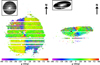 |
Fig. 1 Maps of the polarization angle in degrees, measured relative to north, with B_HIGH filter. Left: NGC-3351 with the approximate location of SN 2012aw marked with a black cross. Right: NGC-4424 with the approximate location of SN 2012cg marked with a black cross. The patterns displayed are compatible with polarization due to the scattering of light of a dominating central source inside a dusty medium (see Appendix A). Milky Way stars are indicated with white circles. A flux image of the galaxies, using the same filter, is presented at the top left corner of each map. |
3 Dust scattering and absorption
In this section, we discuss the general expected polarization patterns from the two main processes of dust scattering and dust absorption. In the first case of dust scattering, as seen in observations (Scarrott et al. 1996) and supported by Monte Carlo radiative transfer (MCRT) simulations (Peest et al. 2017), a dominant light source at the center of a dust medium produces scattered light, whose polarization angle along the LOS is expected to be perpendicular to the direction of emission, resulting in a circular, axisymmetric pattern around the illuminating region(s). Fig. A.1 illustrates this situation for two simple models simulated using the radiative transfer code SKIRT (Baes et al. 2011; Camps & Baes 2015, more information about these models is provided in Appendix A). In optically thick media, this pattern may erode as a result of multiple scattering and consequent depolarization. Due to lower flux levels (less light scattered into the LOS) and lower polarized fraction, randomization of the polarization angle is bound to be more spatially frequent, as seen in Fig. A.1b. At locations with sufficient flux entering the LOS, polarization rotations due to multiply scattered rays should cancel out, and the polarization angle pattern should be maintained. Likewise, if other comparably luminous light sources in the field are present, the pattern will erode because of randomization by the mixing of light from different sources in the LOS. Fig. 1 provides polarization angle maps for NGC-3351 and NGC-4424 from our dataset, whose patterns are compatible with polarization due to scattering.
It is also important to mention that the wavelength dependence of the polarization degree for pure scattering is not universal (as often assumed; see, e.g., Andersson et al. 2013 or Patat et al. 2015) and will follow different trends according to the dust characteristics, as shown in the MCRT simulation of Figure 2. There is no single empirical scattering law to model the observational data. Interestingly, in the case of a typical MW dust mix (see Appendix A), the polarization reaches a minimum within the optical region (~0.61 µm) which we observed with our data. Furthermore, the wavelength dependence of the polarization angle is expected to be mostly constant in the optical region for pure scattering, as seen below in the Fig. 2.
In the second case of dust absorption, in the optical and NIR regimes, χ is expected to track, in optically thick LOSs, the magnetic field that aligns the grains. A medium composed of spheroidal dust grains embedded in an external magnetic field is expected to show partial grain alignment, with the shorter axis parallel to that field (Su et al. 2013) (the grains may rotate around that axis). This alignment leads to the preferential absorption of ultraviolet (UV) and/or optical light for the light component parallel to the longer axis (perpendicular to the magnetic field), which in turn results in the polarization of the detected light being parallel to the magnetic field. Conversely, the absorbed energy is then reemitted in MIR and/or FIR wavelengths with polarizations perpendicular to the magnetic field. In edge-on (or close to) galaxies, χ has been observed to be parallel to the disk (Scarrott et al. 1996; Montgomery & Clemens 2014); while in face-on galaxies, χ appears to follow the direction tangential to the arms (Scarrott et al. 1991). Up to now it has been difficult to make definite predictions due to a general lack of knowledge of the galactic magnetic field structure at both large (dynamo effect) and local scales (flow of charged particles). Moreover, in the face-on case, similar polarization orientation patterns may result from both absorption and scattering processes (Scarrott et al. 1991; Peest et al. 2017). Differentiating between them would then require a spatially comprehensive wavelength dependence analysis of both the polarization fraction and angle.
In fact, as mentioned earlier, the dependence of the polarization degree p with wavelength λ for dust alignment generally follows an empirical Serkowski law (Serkowski 1973):
![Mathematical equation: $p\left( \lambda \right) = {p_{max}}\,\exp \,\left[ { - {k_p}\,{{\ln }^2}\left( {{\lambda \over {{\lambda _{max}}}}} \right)} \right],$](/articles/aa/full_html/2025/11/aa54061-25/aa54061-25-eq10.png) (6)
(6)
where pmax is the maximum polarization degree, λmax is the wavelength at which pmax occurs, and kp gives the width of the curve and is empirically connected to λmax (Wilking et al. 1982) through
 (7)
(7)
with λmax expressed in microns. λmax is known to be connected to the size of dust grains in the medium (Draine 2011) and has been shown to correlate linearly with the total-to-selective extinction ratio, or “reddening law” RV (Serkowski et al. 1975; Vrba et al. 1993), which expresses the interstellar dust-induced starlight reddening. It is defined as
 (8)
(8)
where AV is the total extinction in the V band and EB−V is the color excess, or selective extinction (EB−V = AB − AV), of the V band relative to the B band. Spectropolarimetric studies of different star regions found a relation of RV with the maximum wavelength of polarization (Serkowski et al. 1975; Whittet & van Breda 1978; Clayton & Mathis 1988; Vrba et al. 1993; Andersson & Potter 2007) on the order of
 (9)
(9)
where λmax is expressed in microns. However, in some other regions, no such relation has been confirmed (Whittet et al. 2001; Bagnulo et al. 2017). Whittet et al. (2001) suggest that this may be due to the variation in the alignment of dust grains of different sizes in those regions. For the purpose of this study, we assumed an effective alignment of the grains and employed the relation found by Whittet & van Breda (1978):
 (10)
(10)
The relation expressed by Eq. (6) should appear in regions with little contribution from the light of surrounding sources scattered into the LOS. In Fig. 3, b_HIGH isophotes of NGC-4424 are overlaid with an arrow field, showing the v_HIGH polarimetry of regions where the Serkowski relation provides a good fit (see Section 4) to the wavelength dependence of the polarization degree. In the figure, we can also see that most of this polarization appears tangentially oriented to the outer structure. Comparing with Figs. 1 (right) and A.1, we can see that some of the gaps in the scattering signature of Fig. 1 (right) match the areas where the Serkowski relation provides a good fit. The wavelength dependence of polarization due to absorption by dust grains is clearly different from the scattering case (see Fig. 2), offering a means to disentangle both effects. Some examples of Serkowski laws fit to our data are shown in Fig. 4. However, when multiple dust clouds are present in the LOS and consist of dust with different properties, a simple Serkowski relation may not apply, and extra care is required to model these cases (Patat et al. 2010; Mandarakas et al. 2025). More generally, both scattering and absorption may contribute to a polarized signal, resulting in an unexpected polarization degree- and angle-dependence on wavelength. Separating their contributions is not a trivial task.
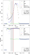 |
Fig. 2 Scattering-wavelength dependence of the spatial average of the polarization degree (upper) and the polarization angle relative to the radial direction (lower) from radiative transfer simulations of a bright source with Ts = 3500 K located at the center of dusty media. These are composed of: silicates (blue triangles), graphites (yellow circles), and polycyclic aromatic hydrocarbons (green squares), as well as the BARE-GR-S dust mixture of the three compounds (Zubko et al. 2003, black stars). The shaded area indicates the optical wavelength range, and the red line indicates the peak wavelength, λp = 0.828 µm, of the emitting sources. |
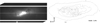 |
Fig. 3 b_HIGH photometry (Left) and isophotes of NGC-4424 overlaid by an arrow field showing the v_HIGH polarimetry of regions where the Serkowski relation provides a good fit (Right). The length of the arrows is proportional to the polarization degree, while their orientation indicates the polarization angle (relative to north). |
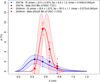 |
Fig. 4 Two different Serkowski relations illustrating the effect of each parameter on the curve. pmax yields the maximum polarization degree and occurs at λ = λmax, while kp relates to the width of the curve. The blue and red lines represent Serkowski models for the vicinities of 2007le and 2006cm, respectively, while the same colored symbols indicate the polarimetry, which yielded those models. The shaded areas indicate the 1σ confidence interval of the model predictions. |
4 Analysis
For each galaxy, we visually inspected the 2D maps of the polarization degree p and angle χ, searching for clear signatures of polarization arising from scattering into the LOS, or from absorption by aligned dust grains, in the spatial distribution of χ, as described in Section 3. We also looked at the relationship between the polarization degree p and the effective wavelength λc of the measurement-band filters across different regions of the galaxies, including those whose polarization is dominated by scattering and those without scattering signatures in their polarization maps. We began by analyzing bins of 5 × 5 pix2, with the projected length of these bins spanning from 0.06 kpc to 0.45 kpc, depending on the galaxy. The photopolarimetric parameters, p and χ, of the vicinity of SNe for each band are provided in Appendix E, together with the respective median polarimetry of the HGs. We then repeated the analysis with bins of 25 × 25 pix2. In each case, if the bin containing the coordinates of the SN could not be successfully fit with a Serkowski law, our RV estimate was based on the average of neighbors at a Manhattan distance of 1 bin.
In each of the cases mentioned above, we performed a robust fitting of a Serkowski relation. This was achieved by first sampling the estimates of the regions defined by p(λ) ± σ(p(λ)) at each band 10 000 times, with each point in the sample assigned a weight, w = 1/σ2(p(λ)). The nonlinear least-squares algorithm “port” within the function nls (Bates & Watts 1988; Chambers & Hastie 1992) of the stats R library was used. This algorithm requires defining initial values and bounds for the model parameters. The initial values for the Serkowski parameters were set according to the data: pmax as the maximum of p measured across the four wavebands, λmax as the λc of the waveband containing the maximum of p within the sample, and kp = −0.1 + 1.86 λmax (following (Wilking et al. 1982)). The following bounds were also defined: 0.000001 ≤ pmax ≤ 1 and λmax ≥ 0.01 µm. We added, in quadrature to the fitting uncertainty, the median measurement uncertainty and the median of the full-width at half-maximum, respectively. In Fig. 4 we plot two Serkowski relations. The fit parameters were obtained in this analysis for the vicinities of 2007le in NGC-7721 and 2006cm in UGC-11723.
Our next goal was to estimate the RV in the projected vicinity of the hosted SNe using the fits for the different bin selections of the HGs. Since our estimates relied on the Serkowski relation given by Eq. (10), and scattering effects could obfuscate our estimates, we employed a set of criteria to select the parameters that best fit a pure Serkowski relation, namely:
λmax must be within the range of the observations, which in our case is 0.388 ≤ λmax ≤ 0.870 µm (which is equivalent to 2.17 ≤ RV ≤ 4.87 according to Eq. (10));
λmax/σ(λmax) > 5;
kp > 0;
the correlation between the Serkowski model predictions,
 , and the measurements must exceed 0.75:
  ; and
; andthe mean normalized absolute residuals between the best model and the data must be less than 25%:
 (11)
(11)
The first two criteria are soft filters, meaning that a fit not satisfying these conditions was still retained for later inspection and used for spatial inferences. The last three criteria ensure that the polarization follows a Serkowski relation. The estimates for an SN, based on each bin selection, were then compared; in all cases the selection based on fewer and smaller bins was favored, as it better represents the vicinity of SNe.
This procedure was used to estimate RV at the approximate locations of four of the 11 SNe in our sample, namely SNe 2006cm, 2007fb, 2007le, and 2011iv. The estimate for the location of SN 2007le, the mean of the fit parameters of the two neighboring 5 × 5 pix2 bins was used. For SNe 2006cm, 2007fb, and 2011iv, the estimates are derived from the 25 × 25 pix2 bins of their coordinates. The results are presented in Table 2.
To obtain an RV estimate for the remaining locations of SNe (2001da, 2002ha, 2003dt, 2007le, 2007on, 2010ev, 2012aw, and 2012cg), for which no bin or neighboring bins provided an accurate Serkowski estimate, we employed INLA (Rue & Martino 2009; Bachl et al. 2019) to spatially infer from sparse bin maps of λmax and RV the values at the positions of SNe. INLA is an approximate Bayesian inference method that accounts for spatial correlations between observed data points not only to predict spatial intermediate unobserved points, but also to correct noisy observations while assigning a variance to its predictions. It has already been shown that INLA can recover structures in scalar and vector fields with high fidelity from sparse sets of observations, while remaining robust to noise injections (González-Gaitán et al. 2019; Rino-Silvestre et al. 2022; Smole et al. 2023). With INLA, it is also possible to infer structures never seen before (Guilherme-Garcia et al. 2023). In Fig. 5, we provide an example of the spatial inference performed by INLA on a map of λmax. For a more detailed comparison between the RV values inferred from Serkowski fits and INLA reconstructions, as well as the choice of the best RV for each position of the SNe, we refer to Appendix C.
Estimates of λmax and RV in the vicinity of SNe.
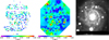 |
Fig. 5 Left: λmax map for NGC-3244, obtained by fitting Serkowski laws to each 5 × 5 pix2 bin and filtering the results of those fits using the criteria defined in Section 4. Center: λmax map inference performed by INLA on the λmax map on the left. Right: b_HIGH pointing image of NGC-3244 (MW field star regions were masked during the data reduction process). All images are presented at the same spatial scale. |
5 Results and discussion
5.1 Comparison of RV estimates from photopolarimetry and from SN light curves
The obtained RV values range from 2.51 ± 0.39 to 3.94 ± 0.99 with a median of 3.34 ± 0.97. This result is consistent with the average RV ≈ 3.1 extinction law of the Milky Way (Cardelli et al. 1989; O’Donnell 1994) and distinct from RV ≈ 1.7 associated with very reddened Type Ia SNe (Burns et al. 2014). However, the RV estimated through the LC analysis (Mandel et al. 2011; Phillips et al. 2013; Burns et al. 2014; Amanullah et al. 2015; Gutiérrez et al. 2016) for some of the SNe in our sample (2001da, 2006cm, 2007fb, 2007le, 2007on, 2010ev, and 2012cg) place them into this category of very reddened SNe (see Column 2 of Table 3).
Our RV values, estimated using photopolarimetry, are assigned to a median projected area of 0.029 ± 0.022 kpc2, corresponding to a squared vicinity with a length of ~ 170 pc, which are much larger than the typical scale of an H II region (~30 pc). This means that the properties inferred for these bins may likely be averages of different dust structures and scatterings. In Appendix B we test our fitting technique with simulated data and find that our RV estimates may be underestimated by as much as ∆RV ~ 0.4, further increasing the difference with the values directly obtained from the SNe.
As shown in Fig. 6 and Table 3, the RV obtained from photopolarimetry differ by up to 2.46σ from the estimates derived from previous LC analyses of SNe (Mandel et al. 2011; Phillips et al. 2013; Burns et al. 2014; Amanullah et al. 2015; Gutiérrez et al. 2016). The values obtained by Amanullah et al. (2015) at different epochs of SN 2012cg suggest that RV varies with time after peak luminosity (in the B band). This had already been demonstrated for the sample of SNe studied by Förster et al. (2013), who proposed two possible scenarios: multiple scattering processes due to the presence of CSM (Amanullah & Goobar 2011), or the progressive destruction of sufficiently nearby material (Förster et al. 2013), which would lead to a change in reddening over time. Moreover, a photometric data analysis by Bulla et al. (2018) showed that 15 of the 48 SNe had a time-variable EB−V. They predicted that the dust responsible for that variation was within the CSM range for four SNe and was part of the nearby patchy ISM for the remaining 11. Our photopolarimetric data lack the spatial resolution necessary to assess the evolution of the CSM of SNe in the years following the explosion (the data were obtained in 2017). However, it is worth noting that not a single area within our galaxies is consistent with such small RV values, as found for these peculiar SNe Ia.
Indeed, comparing the RV estimates at the vicinities of of SNe to the median RV, < RV >5, of the HGs (provided in Table 4 and Fig. 7), we observe that the estimates for all vicinities of SNe fall below 1σ of the HG median. Moreover, comparing to all other regions of a given galaxy (see, e.g., Fig. 8), we see that the RV values in different locations span mostly between ~2.5–4, as in the MW, and not below. This is true for all galaxies in our sample (see Appendix D). These results provide further evidence that there is nothing unusual at the extended site around these SNe, and that no regions in the galaxies follow the peculiar low RV reddening laws found for some highly extincted SNe Ia. This further supports the hypothesis that either the average dust properties of more extended regions are not representative of more localized individual ISM clouds, or that the explosion of SNe interacts with the nearby environment, thereby altering its dust properties (see, e.g., Hoang et al. 2019).
It is important to note that as SNe are energetic back-illuminators, the typical depth of the dust layer probed with galaxy observations might indeed be much shallower than with SNe. In spiral galaxies, the magnetic fields in the thin disk are known to be stronger and more ordered than in the thick disk, and perhaps even oriented differently (e.g., Beck 2001). The effects of less dust and more randomly aligned grains reduce the overall degree of polarization in shallower observations, but the wavelength dependence should not change in principle if the dust grain composition and size distribution remain unchanged, and the alignment maintains a component perpendicular to the observer. This is statistically valid, but as shown in Mandarakas et al. (2025) multiple dust clouds may occasionally have different properties and induce erroneous Serkowski relations if they are treated as a single component.
Comparison between published RV from data of SNe and our estimates in the vicinity of SNe within the host.
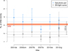 |
Fig. 6 Comparison of RV estimated in the vicinity of SNe with estimates from direct observations of SNe. Blue dots are estimates obtained using late-time (several years post maximum light) multiwaveband photopolarimetry in the vicinity of SNe. Black squares are estimates based on model fitting to color LC data of those SNe (Mandel et al. 2011; Phillips et al. 2013; Burns et al. 2014; Amanullah et al. 2015; Gutiérrez et al. 2016). The median, and its uncertainty, of each estimation are presented by dashed lines in the corresponding color. The fiducial RV for the Milky Way is presented by a red line with its uncertainty being the shaded orange area. A 2.5σ separation is observed between the median of RV estimates obtained with photopolarimetry and with LC data. |
Host Galaxy and RV estimates of SNe.
5.2 RV relations with galaxy properties
Despite our small sample of SNe, we attempted to investigate possible relationships between the RV measured in the vicinity of SNe, the difference between the measured RV and the < RV > of the HG (i.e., ∆RV(σ)), and the properties of the HGs of SNe. We thus extracted and/or derived from the Asiago Supernova Catalogue6 and from NED7 the following: morphology (Hubble T-type), normalized galactocentric distance, normalized directional light radius (NDLR) (Gupta et al. 2016), and galactic inclination. In addition, from stellar population fits to multiband photometry carried out by González-Gaitán et al. (2025), we obtained the global and local (0.5 kpc radius vicinity) stellar mass, stellar age, dust attenuation AV, dust index,  8, star formation rate (SFR), and specific SFR for seven out of the nine galaxies in our data (all except for NGC-1404 and NGC-3244). Of all the investigated pairs of properties and with seven data points (seven SNe), no property presents a correlation greater than 0.7 with our RV estimates in the vicinity of SNe. With five data points (excluding the SNe in NGC-1404 and NGC-3244), we also find correlations with RV greater than 0.7 for the HG stellar age and dust index (Figs. 9, 10, respectively). Despite the large uncertainties in the parameters and the small sample size, increasing trends are observed in each case.
Additionally, for each galaxy in our sample, we selected all bins, whose fit to the Serkowski relation matched our filtering criteria (see Section 4), and compared the relationship between RV and the projected galactocentric offset. Again, we find no relationship between these parameters, despite the presence of some extreme outliers (illustrations of these results can be found in Appendix D). Given that, for photometric data fit to stellar population models, the dust attenuation law is highly dependent on scattering and geometric effects and thus shows a decreasing trend with galactocentric distance (see Figs. 11–15 of Duarte et al. 2025 or Fig. 6 of Hutton et al. 2015). This is a reassuring result: polarimetric data carefully fit to Serkowski laws is perhaps more appropriate to infer dust reddening than intensity data fit to stellar population models. It provides a cleaner way to probe the real RV and the actual physical properties of the dust.
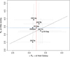 |
Fig. 7 Median RV in the vicinity of the hosted SNe versus the median RV for the present sample of hosts of SNe, < RV >. The dashed red line marks the median of the HGs < RV >, while the dashed blue line indicates the median of the RV in the vicinity of SNe. The black line represents an ideal 1:1 relation. |
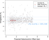 |
Fig. 8 RV estimated for each 5 × 5 pix2 bin versus the projected galactocentric offset (gray diamonds) for NGC-1404. The dashed blue lines mark the median RV, < RV >, and the short dashed blue lines enclose the 1σ uncertainty of the median. The red dot indicates the estimate and/or inference obtained for the vicinity of the hosted SNe. The average uncertainty of RV across bins is 0.42, and each bin has a projected length of 23 pc. For other galaxies in the sample, see Appendix D. |
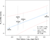 |
Fig. 9 RV estimations in the vicinity of SNe versus HG stellar age (expressed in gigayears). The legend presents the fitting parameters following y = mx + b, as well as the correlation, corr, between the properties; the mean normalized residuals of the fit, Nresd; and the coefficient of determination of the fit, R2. The dashed blue line presents the linear fit, while the dotted red lines provide the lσ uncertainty interval of the fit. |
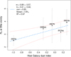 |
Fig. 10 RV estimations in the vicinity of SNe versus the HG dust index. The same key as shown in Fig. 9. |
6 Concluding remarks
Using galaxy multiwaveband (BVRI) photopolarimetry, we analyzed nine HGs of 11 SNe, most of which are highly extincted SNe Ia with very peculiar dust reddening laws. By finding regions that are well fitted by a Serkowski polarization-wavelength relation and are thus mainly driven by dust extinction and grain alignment (rather than scattering), we obtained the wavelength of maximum polarization. We assumed that the wavelength of maximum polarization relates to the reddening law parameterized with RV (see, e.g., Whittet & van Breda 1978), but we caution that this relation may not be universal (see, e.g., Bagnulo et al. 2017). By binning different regions and using spatial inference when necessary, we obtained RV in the vicinity of SNe and across the galaxies. We find no evidence of peculiar extinction laws in the 0.1–3 kpc vicinity of these reddened SNe Ia. The RV values are consistent with the average value of the MW, and they are representative of the entire HG. However, they are significantly different (~2.5σ) from the values obtained directly from the light of SNe around maximum.
Our results match the RV values from HG intensity analysis at the site of SNe before explosion (Hutton et al. 2015), as well as RV estimates from late-time observations of SNe (10–20 days after maximum light by Amanullah et al. 2015, or after 35 days by Förster et al. 2013) for the same SNe Ia. A viable explanation for this discrepancy is the interaction of the light of SNe with the immediate neighboring material, such as CSM or patchy ISM, which occurs in explosions within very dusty environments (Förster et al. 2013; Hoang 2017; Bulla et al. 2018).
This study demonstrates the independent and powerful capabilities of photopolarimetry to obtain dust properties in various systems. Care should be taken regarding contamination from polarization caused by scattering and/or the effects of multiple clouds with differing dust properties in the LOS (Patat et al. 2010; Mandarakas et al. 2025), the latter scenario being likely when observing with coarser spatial resolution. While spectropolarimetry has been used to study Type Ia SNe and the material along their LOS (e.g., Patat et al. 2015; Cikota et al. 2017; Zelaya et al. 2017; Shrestha et al. 2025; Nagao et al. 2024), the use of spatially resolved, multiwaveband photopolarimetry of the surrounding galactic environment remains scarce. This complementary approach provides important constraints on the average physical properties of the interstellar material near the SN and across the galaxy. Progress in the inclusion of polarization effects due to dichroic absorption in radiative transfer codes will allow for a more accurate modeling of SNe and their HGs.
Acknowledgements
João Rino-Silvestre was supported by FCT (PD/BD/150487/2019), through the IDPASC (https://idpasc.lip.pt/) PhD program. The work here described was supported by the CRISP project (PTDC/FIS-AST/31546/2017). CENTRA – Center for Astrophysics and Gravitation, thanks the support by FCT via Grant Project No. UIDB/00099/2020. We would like to thank Takashi Nagao, for his insights on different features of the polarization of light by interactions with dust grains, and Maarten Baes for his help and instruction with SKIRT. This research has used the NASA/IPAC Extragalactic Database (NED), which is funded by the National Aeronautics and Space Administration and operated by the California Institute of Technology. This research has made use of the Asiago Supernova Catalogue (Barbon et al. 1999). This work has used data from the European Space Agency (ESA) mission Gaia (https://www.cosmos.esa.int/gaia), processed by the Gaia Data Processing and analysis Consortium (DPAC, https://www.cosmos.esa.int/web/gaia/dpac/consortium). Funding for the DPAC has been provided by national institutions, in particular, the institutions participating in the Gaia Multilateral Agreement. This project used public archival data from the Dark Energy Survey (DES). Funding for the DES Projects has been provided by the U.S. Department of Energy, the U.S. National Science Foundation, the Ministry of Science and Education of Spain, the Science and Technology FacilitiesCouncil of the United Kingdom, the Higher Education Funding Council for England, the National Center for Supercomputing Applications at the University of Illinois at Urbana-Champaign, the Kavli Institute of Cosmological Physics at the University of Chicago, the Center for Cosmology and Astro-Particle Physics at the Ohio State University, the Mitchell Institute for Fundamental Physics and Astronomy at Texas A&M University, Financiadora de Estudos e Projetos, Fundação Carlos Chagas Filho de Amparo à Pesquisa do Estado do Rio de Janeiro, Conselho Nacional de Desenvolvimento Científico e Tecnológico and the Ministério da Ciência, Tecnologia e Inovação, the Deutsche Forschungsgemeinschaft, and the Collaborating Institutions in the Dark Energy Survey. The Collaborating Institutions are Argonne National Laboratory, the University of California at Santa Cruz, the University of Cambridge, Centro de Investigaciones Energéticas, Medioambientales y Tecnológicas-Madrid, the University of Chicago, University College London, the DES-Brazil Consortium, the University of Edinburgh, the Eidgenössische Technische Hochschule (ETH) Zürich, Fermi National Accelerator Laboratory, the University of Illinois at Urbana-Champaign, the Institut de Ciències de l’Espai (IEEC/CSIC), the Institut de Física d’Altes Energies, Lawrence Berkeley National Laboratory, the Ludwig-Maximilians Universität München and the associated Excellence Cluster Universe, the University of Michigan, the National Optical Astronomy Observatory, the University of Nottingham, The Ohio State University, the OzDES Membership Consortium, the University of Pennsylvania, the University of Portsmouth, SLAC National Accelerator Laboratory, Stanford University, the University of Sussex, and Texas A&M University. Based in part on observations at Cerro Tololo Inter-American Observatory, National Optical Astronomy Observatory, which is operated by the Association of Universities for Research in Astronomy (AURA) under a cooperative agreement with the National Science Foundation.
Appendix A SKIRT models
Stellar Kinematics Including Radiative Transfer (SKIRT) (Baes et al. 2011; Camps & Baes 2015) is a MCRT suite that offers some built-in source templates, geometries, dust characterizations, spatial grids, and instruments, as well as an interface so that a user can easily describe a physical model. The user can in this way avoid coding the physics that describes both the source (e.g., AGN or galaxy type, observation perspective, emission spectrum) and environment (between the simulated source and observer, such as dust grain type and orientation, dust density distribution, etc.) but instead, design a model of modular complexity by following a Q&A prompt (itself adaptable to the user expertise).
To demonstrate the spatial polarization angle pattern, displayed in Fig. A.1, that signals scattering as the dominant process in polarizing the light that comes into the LOS, we constructed a simple, one source one medium model. The details of the model are given below, while a ready-to-run SKIRT input file and scripts to process the simulation outputs are publicly available.
The light source is modeled by a spherical Gaussian geometry of the form.
 (A.1)
(A.1)
with σ = 0.05 kpc, with a black body emission spectrum with temperature T = 3500K. The medium is modeled by a homogeneous sphere with radius r = 0.5kpc and by dust properties that replicate those of a mixture of silicates, graphites, and polycyclic aromatic hydrocarbons with composition and size distributions that accurately replicate the extinction, emission and abundances constraints for the Milky Way (Camps et al. 2015; Gordon et al. 2017), based on the BARE-GR-S dust model by Zubko et al. (2003).
In one simulation the total dust mass is normalized to achieve an optical depth9, at λ =0.35 µm and along length of 1 kpc, of τ = 1. In the other simulation, to increase the fraction of light reaching the LOS through multiple instances of scattering, the optical depth was increased to τ = 5.
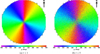 |
Fig. A.1 Polarization angle in degrees, measured relative to north, as well as maps at λ = 228.5 nm for two simulations of an emitting spheroidal source inside an isotropic, homogeneous spherical dust medium. The optical depth, τ, of the medium of the simulation on the right is five times greater than that of the one on the left. This results in more multiple light scattering before it reaches the LOS, leading to randomization of the polarization angle pattern and depolarization. |
Appendix B Fitting simulated Serkowski laws
In this section, we test our fitting methodology with the following Monte Carlo simulation: we generate Serkowski laws in a grid of 0.1 < pmax < 8% and 0.3 < λmax < 0.8 µm values, for which we obtain simulated polarization data by randomly sampling the polarization values of the generated Serkowski law assuming a 1-sigma uncertainty of 50% for each measurement, which roughly corresponds to our measured uncertainties. For every pmax and λmax realization we generate 100 simulated observations in UBVRI bands and then fit the data with a Serkowski law with and without U-band to recover the fitted pmax, λmax and compare them to the simulated values. The results are shown in Figure B.1. The median difference in ∆λmax = λmax,fit − λmax,sim is −0.07 µm with a dispersion of 0.09 µm when using BVRI data. As expected, the inclusion of U-band information decreases the median difference reaching −0.05 µm with 0.07 µm dispersion. These differences in maximum wavelength translate to a systematic offset in RV of ∆RV = −0.39 ± 0.52 for BVRI and ∆RV = −0.20 ± 0.37 for UBVRI. Our simulation thus suggests that all our RV measurements should be corrected by adding ~ 0.4, which only exacerbates the discrepancies with the values for SNe.
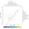 |
Fig. B.1 Difference between fitted and simulated maximum wavelength of polarization, ∆λmax = λmax,fit − λmax,sim using fits to UBVRI vs. only BVRI data. The size of the points represent the simulated pmax, while the colors represent the simulated λmax. The histograms show the distribution of both differences with the median and deviation shown in solid and dashed lines. |
Appendix C Choosing RV estimates
The fitting procedure described in Section 4 succeeded in providing Serkowski relations, and thus provide reliable RV estimates, for the vicinity of SNe 2001da, 2006cm, 2007le and 2011iv. This, however, was not the case for the vicinity of SNe 2002ha, 2003dt, 2007fb, 2007on, 2010ev, 2012aw and 2012cg. In the cases of SNe 2012aw and 2012cg, this was expected given that the polarization angle maps of their HG, NGC-3351 and NGC-4424, present (in some wavebands) strong indications of scattering as the dominant source of polarization (see Fig. 1). This is reflected in the percentage of bins successfully fit and within all our criteria (percentage of success, or PoS). The median PoS, across galaxies, is 16 ± 3% while the PoS for NGC-3351 and NGC-4424 are 1% and 7%, respectively.
As for the case of the SNe within NGC-6962, 2002ha and 2003dt, their locations unfortunately coincided with the gap between the two chips of the CCD. SN 2007on is located on the outskirts of NGC-1404, a region where the flux level, unfortunately, matched the background and was therefore rejected.
Although an estimate directly from the bin with the location of SN 2011iv, in NGC-1404, was not possible, we were able to use two well-fitted neighboring bins from which we took the mean of their RV values. For SN 2001da, even though the estimated λmax falls within expectations, this fit is based on polarization values whose uncertainty makes them consistent with p = 0%. Therefore, these results are also unreliable.
In an attempt to obtain an RV estimate for the vicinity of those SNe where the fitting procedure (Section 4) failed, and also to improve the estimates previously obtained (SNe 2001da, 2006cm, 2007le, 2011iv), we employ INLA to perform spatial inference on the λmax and RV maps obtained in the previous step. As the uncertainty of the inference, we add in quadrature the INLA output standard deviation for the inference together with the median uncertainty of the input map. We perform equivalent inferences of the RV at locations of SNe that had already been successfully estimated and shown in Tab. 2. We find virtually no tension between the RV values obtained directly from spatial inference and those obtained by applying Eq. (10) to the spatial inferences performed on the λmax maps. However, the uncertainties for the RV values obtained from the inferred λmax maps are much larger10 than the ones obtained by inference from the RV maps, for that reason we chose to use these last ones instead. For more details on the results obtained with INLA see Tab. C.1.
To verify the validity of the inferences made with INLA, the differences ∆RV, between the inferred RV values and those obtained directly with the Serkowski fits were calculated. The results, given in units of σ and presented in Tab. C.2, show the RV to be within 0.75σ of the estimates based on bins with size 5 × 5 pix2 and with size 25 × 25 pix2. We then analyzed the neighborhood of SNe in the 5 × 5 pix2 bin map, to decide whether to use the estimates based on the 25 × 25 pix2 bins or the inferences of RV obtained with INLA.
RV estimates of SNe inferred using INLA.
SN 2007Ie
The mean RV across bins (D1 neighbours) estimated for the vicinity of SN 2007le is very similar to the value inferred with INLA and, despite a lack of 5 × 5 pix2 bins well fitted nearby, within the corresponding 25 × 25 pix2 bin area the estimates of RV are also very similar. Therefore, we chose to take the value inferred with INLA, RV = 3.18 ± 0.83, as it reports to a smaller area while taking into account information from its surroundings.
SN 2006cm
The corresponding 5 × 5 pix2 bin estimate did not pass the selection criteria. Within the neighborhood at a distance of 1 bin, we find only one reasonable estimate (λmax = 0.487 ± 0.065 µm) and two outliers without credibility (λmax = {0.02 ± 0.10, 0.1 ± 4.5} µm). For this reason, we prefer to use the RV estimated from the 25 × 25 pix2 bin (see Tab. 2) over any estimate obtained from 5 × 5 pix2 bins. Looking further into the 5 × 5 pix2 bins that make up the 25 × 25 pix2 bin, we find 10 other successfully fitted bins, three of them without credibility (λmax = {1.63 ± 0.73, 0.02 ± 0.16, 0.01 ± 0.24} µm) and the remaining 7 with RV = {2.81 ± 0.39, 3.19 ± 0.40, 3.33 ± 0.40, 3.43 ± 0.41, 3.46 ± 0.41, 3.58 ± 0.41, 3.42 ± 0.41}. The RV estimated from the 25 × 25 pix2 bin is not only the result of missing polarimetric data for the filter R_SPECIAL, and previously statistically rejected flux data, but also indicates a mixture of properties of the different spatial sections within it. For these reasons, even though the ∆σ between the direct estimate and the INLA inference is below 1 (see Tab. C.2) and the inference presents a greater uncertainty, we chose to adopt the RV inferred by INLA, RV = 2.59 ± 0.60.
SN 2001da and 2011iv
The corresponding 5 × 5 pix2 bins did not pass our selection criteria either. At a distance of 1 bin not a single credible estimate is found, only outliers with λmax well beyond the scope of application of the Serkowski relation which would physically imply a drastically different dust grain size distribution from what has been previously predicted by different models (Calzetti et al. 2000; Zubko et al. 2003) for dust in the ISM. The diversity of the neighborhood may be intrinsic in this case, since the center of each bin stands at ~ 450 pc for 2001da, and ~ 120 pc for 2011iv, from their closest neighbors (far beyond the H II region scales), or it may be a manifestation of poor SNR and/or resolution, where properties from different regions may be mixed. The RV estimates based on the 5 × 5 pix2 bins were then rejected due to a lack of credibility in the fit to the Serkowski relation in the SN bin and to the diversity of values in the neighborhood. However, the fact that the RV estimates for the 25 × 25 pix2 bins are incompatible with any of the bins that fit inside them points toward a mixture of properties due to a loss in spatial resolution, as mentioned above. Additionally, in the case of SN 2001da the uncertainty of the reduced polarization degree at all measured bands is consistent with 0. For these reason, we chose to adopt the values inferred by INLA, RV = 3.94 ± 0.99 for 2001da, and RV = 3.23 ± 0.79 for 2011iv.
RV differences.
Appendix D Host galaxy IGM RV versus projected galactocentric offset
In the following figures we plot, for each galaxy in our sample, the total-to-selective extinction ratio versus the projected galactocentric offset of each 5 × 5 pix2 bin which fit to a Serkowski relation matched all our filtering criteria (see Section 4). Unlike (Hutton et al. 2015), we do not find a relation between these two properties.
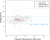 |
Fig. D.1 RV estimated for each 5 × 5 pix2 bin versus the projected galactocentric offset, for NGC-3244. The same key as in 8 is provided. The average uncertainty of RV across bins is 0.42, and each bin has a projected length of 34 pc. |
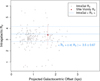 |
Fig. D.2 RV estimated for each 5 × 5 pix2 bin versus the projected galactocentric offset, for NGC-3351. The same key as in 8 is provided. The average uncertainty of RV across bins is 0.41, and each bin has a projected length of 12 pc. |
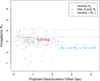 |
Fig. D.3 RV estimated for each 5 × 5 pix2 bin versus projected galac-tocentric offset, for NGC-4424. The same key as in 8 is provided. The average uncertainty of RV across bins is 0.42, and each bin has a projected length of 17 pc. |
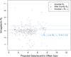 |
Fig. D.4 RV estimated for each 5 × 5 pix2 bin versus projected galac-tocentric offset, for NGC-6962. The same key as in8 is provided. The average uncertainty of RV across bins is 0.023, and each bin has a projected length of 68 pc. |
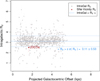 |
Fig. D.5 RV estimated for each 5 × 5 pix2 bin versus projected galac-tocentric offset, for NGC-7721. The same key as in 8 is provided. The average uncertainty of RV across bins is 0.41, and each bin has a projected length of 25 pc. |
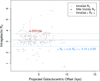 |
Fig. D.6 RV estimated for each 5 × 5 pix2 bin versus projected galac-tocentric offset, for NGC-7780. The same key as in 8 is provided. The average uncertainty of RV across bins is 0.41, and each bin has a projected length of 90 pc. |
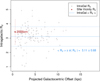 |
Fig. D.7 RV estimated for each 5 × 5 pix2 bin versus projected galac-tocentric offset, for UGC-11723. The same key as in 8 is provided. The average uncertainty of RV across bins is 0.41 and each bin has a projected length of 87 pc. |
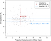 |
Fig. D.8 RV estimated for each 5 × 5 pix2 bin versus projected galac-tocentric offset, for UGC-12859. The same key as in 8 is provided. The average uncertainty of RV across bins is 0.42, and each bin has a projected length of 91 pc. |
Appendix E Photopolarimetry of SNe
Here, we provide the photo-polarimetric parameters, p and χ, obtained in each band for the vicinity of SNe, using the 5 × 5 and 25 × 25 binned maps, after calibration and reduction. For comparison, we also provide the respective HG median polarization, < p > and < χ >, obtained from those maps, and the respective differences, ∆p and ∆χ.
Polarization degree data, binning 5 × 5 pix2.
Polarization angle data, binning 5 × 5 pix2.
Polarization degree data, binning 25 × 25 pix2.
Polarization angle data, binning 25 × 25 pix2.
References
- Amanullah, R., & Goobar, A. 2011, ApJ, 735, 20 [Google Scholar]
- Amanullah, R., Goobar, A., Johansson, J., et al. 2014, ApJ, 788, L21 [NASA ADS] [CrossRef] [Google Scholar]
- Amanullah, R., Johansson, J., Goobar, A., et al. 2015, MNRAS, 453, 3300 [Google Scholar]
- Andersson, B. G., & Potter, S. B. 2007, ApJ, 665, 369 [NASA ADS] [CrossRef] [Google Scholar]
- Andersson, B. G., Piirola, V., De Buizer, J., et al. 2013, ApJ, 775, 84 [NASA ADS] [CrossRef] [Google Scholar]
- Babusiaux, C., Fabricius, C., Khanna, S., et al. 2023, A&A, 674, A32 [NASA ADS] [CrossRef] [EDP Sciences] [Google Scholar]
- Bachl, F. E. et al. 2019, Methods Ecol. Evol., 10, 760 [Google Scholar]
- Baes, M., Verstappen, J., De Looze, I., et al. 2011, ApJ, 196, 22 [Google Scholar]
- Baes, M., Camps, P., & Kapoor, A. U. 2022, A&A, 659, A149 [NASA ADS] [CrossRef] [EDP Sciences] [Google Scholar]
- Bagnulo, S., Landolfi, M., Landstreet, J. D., et al. 2009, PASP, 121, 993 [Google Scholar]
- Bagnulo, S., Cox, N. L. J., Cikota, A., et al. 2017, A&A, 608, A146 [NASA ADS] [CrossRef] [EDP Sciences] [Google Scholar]
- Barbon, R., Buondí, V., Cappellaro, E., & Turatto, M. 1999, A&AS, 139, 531 [NASA ADS] [CrossRef] [EDP Sciences] [Google Scholar]
- Bates, D., & Watts, D. 1988, Nonlinear Regression Analysis and Its Applications, Wiley Series in Probability and Statistics (Wiley) [Google Scholar]
- Beck, R. 2001, Space Sci. Rev., 99, 243 [NASA ADS] [CrossRef] [Google Scholar]
- Betoule, M., et al. 2014, A&A, 568, A22 [NASA ADS] [CrossRef] [EDP Sciences] [Google Scholar]
- Bohren, C. F., & Huffman, D. R. 1998, Particles Small Compared with the Wavelength (John Wiley & Sons, Ltd), 130 [Google Scholar]
- Brout, D., & Scolnic, D. 2021, ApJ, 909, 26 [NASA ADS] [CrossRef] [Google Scholar]
- Bulla, M., Goobar, A., & Dhawan, S. 2018, MNRAS, 479, 3663 [Google Scholar]
- Burns, C. R., Stritzinger, M., Phillips, M. M., et al. 2014, ApJ, 789, 32 [Google Scholar]
- Calzetti, D., Armus, L., Bohlin, R. C., et al. 2000, ApJ, 533, 682 [NASA ADS] [CrossRef] [Google Scholar]
- Camps, P., & Baes, M. 2015, Astron. Comput., 9, 20 [Google Scholar]
- Camps, P., Misselt, K., Bianchi, S., et al. 2015, A&A, 580, A87 [NASA ADS] [CrossRef] [EDP Sciences] [Google Scholar]
- Cardelli, J. A., Clayton, G. C., & Mathis, J. S. 1989, ApJ, 345, 245 [Google Scholar]
- Chambers, J., & Hastie, T. 1992, Statistical Models in S, Wadsworth & Brooks/Cole Computer Science Series (Wadsworth & Brooks/Cole Advanced Books & Software) [Google Scholar]
- Cikota, A., Patat, F., Cikota, S., Spyromilio, J., & Rau, G. 2017, MNRAS, 471, 2111 [NASA ADS] [Google Scholar]
- Cikota, A., Hoang, T., Taubenberger, S., et al. 2018, A&A, 615, A42 [EDP Sciences] [Google Scholar]
- Clayton, G. C., & Mathis, J. S. 1988, ApJ, 327, 911 [Google Scholar]
- D’Alessio, P., Calvet, N., & Hartmann, L. 2001, ApJ, 553, 321 [Google Scholar]
- Davis, Leverett, J., & Greenstein, J. L. 1951, ApJ, 114, 206 [NASA ADS] [CrossRef] [Google Scholar]
- Draine, B. T. 2011, Physics of the Interstellar and Intergalactic Medium (Princeton University Press) [Google Scholar]
- Duarte, J., González-Gaitán, S., Mourão, A., et al. 2025, A&A, 700, A169 [NASA ADS] [CrossRef] [EDP Sciences] [Google Scholar]
- Farafonov, V. G., Il’in, V., Voshchinnikov, N. V., & Prokopjeva, M. S. 2005, SPIE Conf. Ser., 5829, 117 [Google Scholar]
- Felton, M. A., & Scarrott, S. M. 1997, MNASSA, 56, 51 [Google Scholar]
- Fitzpatrick, E. L. 1999, PASP, 111, 63 [Google Scholar]
- Fitzpatrick, E. L., & Massa, D. 2007, ApJ, 663, 320 [Google Scholar]
- Förster, F., González-Gaitán, S., Folatelli, G., & Morrell, N. 2013, ApJ, 772, 19 [CrossRef] [Google Scholar]
- González-Gaitán, S., de Souza, R. S., Krone-Martins, A., et al. 2019, MNRAS, 482, 3880 [CrossRef] [Google Scholar]
- González-Gaitán, S., Mourão, A. M., Patat, F., et al. 2020, A&A, 634, A70 [NASA ADS] [CrossRef] [EDP Sciences] [Google Scholar]
- González-Gaitán, S., de Jaeger, T., Galbany, L., et al. 2021, MNRAS, 508, 4656 [CrossRef] [Google Scholar]
- González-Gaitán, S., Gutiérrez, c. P., Martins, G., et al. 2025, A&A, 700, A119 [NASA ADS] [CrossRef] [EDP Sciences] [Google Scholar]
- Goobar, A. 2008, ApJ, 686, L103 [CrossRef] [Google Scholar]
- Gordon, K. D., Clayton, G. C., Misselt, K. A., Landolt, A. U., & Wolff, M. J. 2003, ApJ, 594, 279 [NASA ADS] [CrossRef] [Google Scholar]
- Gordon, K. D., Baes, M., Bianchi, S., et al. 2017, A&A, 603, A114 [NASA ADS] [CrossRef] [EDP Sciences] [Google Scholar]
- Guilherme-Garcia, P., Krone-Martins, A., & Moitinho, A. 2023, A&A, 673, A128 [NASA ADS] [CrossRef] [EDP Sciences] [Google Scholar]
- Gupta, R. R., Kuhlmann, S., Kovacs, E., et al. 2016, AJ, 152, 154 [NASA ADS] [CrossRef] [Google Scholar]
- Gutiérrez, C. P., González-Gaitán, S., Folatelli, G., et al. 2016, A&A, 590, A5 [Google Scholar]
- Hall, J. S. 1949, Science, 109, 166 [NASA ADS] [CrossRef] [Google Scholar]
- Hiltner, W. A. 1949, Science, 109, 165 [NASA ADS] [CrossRef] [Google Scholar]
- Hoang, T. 2017, ApJ, 836, 13 [Google Scholar]
- Hoang, T., & Lazarian, A. 2016, ApJ, 831, 159 [Google Scholar]
- Hoang, T., Tram, L. N., Lee, H., & Ahn, S.-H. 2019, Nat. Astron., 3, 766 [Google Scholar]
- Hutton, S., Ferreras, I., & Yershov, V. 2015, MNRAS, 452, 1412 [NASA ADS] [CrossRef] [Google Scholar]
- Jones, A., Wang, L., Krisciunas, K., & Freeland, E. 2012, ApJ, 748, 17 [Google Scholar]
- Kawabata, K. S., Akitaya, H., Yamanaka, M., et al. 2014, ApJ, 795, L4 [Google Scholar]
- Kriek, M., & Conroy, C. 2013, ApJ, 775, L16 [NASA ADS] [CrossRef] [Google Scholar]
- Lazarian, A., & Hoang, T. 2007, MNRAS, 378, 910 [Google Scholar]
- Mandarakas, N., Tassis, K., & Skalidis, R. 2025, A&A, 698, A168 [NASA ADS] [CrossRef] [EDP Sciences] [Google Scholar]
- Mandel, K. S., Narayan, G., & Kirshner, R. P. 2011, ApJ, 731, 120 [CrossRef] [Google Scholar]
- Montgomery, J. D., & Clemens, D. P. 2014, ApJ, 786, 41 [NASA ADS] [CrossRef] [Google Scholar]
- Nagao, T., Maeda, K., Mattila, S., et al. 2024, A&A, 687, L19 [NASA ADS] [CrossRef] [EDP Sciences] [Google Scholar]
- Noll, S., Burgarella, D., Giovannoli, E., et al. 2009, A&A, 507, 1793 [NASA ADS] [CrossRef] [EDP Sciences] [Google Scholar]
- O’Donnell, J. E. 1994, ApJ, 422, 158 [Google Scholar]
- Patat, F. 2005, MNRAS, 357, 1161 [NASA ADS] [CrossRef] [Google Scholar]
- Patat, F., & Romaniello, M. 2006, PASP, 118, 146 [Google Scholar]
- Patat, F., Maund, J. R., Benetti, S., et al. 2010, A&A, 510, A108 [NASA ADS] [CrossRef] [EDP Sciences] [Google Scholar]
- Patat, F., Taubenberger, S., Cox, N. L. J., et al. 2015, A&A, 577, A53 [NASA ADS] [CrossRef] [EDP Sciences] [Google Scholar]
- Peest, C., Camps, P., Stalevski, M., Baes, M., & Siebenmorgen, R. 2017, A&A, 601, A92 [NASA ADS] [CrossRef] [EDP Sciences] [Google Scholar]
- Phillips, M. M., Simon, J. D., Morrell, N., et al. 2013, ApJ, 779, 38 [NASA ADS] [CrossRef] [Google Scholar]
- Plaszczynski, S., Montier, L., Levrier, F., & Tristram, M. 2014, MNRAS, 439, 4048 [NASA ADS] [CrossRef] [Google Scholar]
- Pollack, J. B., Hollenbach, D., Beckwith, S., et al. 1994, ApJ, 421, 615 [Google Scholar]
- Rho, J. et al. 2009, ApJ, 700, 579 [NASA ADS] [CrossRef] [Google Scholar]
- Rino-Silvestre, J., González-Gaitán, S., Stalevski, M., et al. 2022, Neural Comput. Appl., 35, 7719 [Google Scholar]
- Rue, H., & Martino, S. 2009, J. R. Stat. Soc. B, 71, 319 [Google Scholar]
- Scarrott, S. M., Rolph, C. D., Wolstencroft, R. W., & Tadhunter, C. N. 1991, MNRAS, 249, 16 [Google Scholar]
- Scarrott, S. M., Foley, N. B., Gledhill, T. M., & Wolstencroft, R. D. 1996, MNRAS, 282, 252 [Google Scholar]
- Scolnic, D. M., Riess, A. G., Foley, R. J., et al. 2014, ApJ, 780, 37 [Google Scholar]
- Serkowski, K. 1973, in Interstellar Dust and Related Topics, 52, eds. J. M. Greenberg, & H. C. van de Hulst, 145 [Google Scholar]
- Serkowski, K., Mathewson, D. S., & Ford, V. L. 1975, ApJ, 196, 261 [NASA ADS] [CrossRef] [Google Scholar]
- Shrestha, M., DeSoto, S., Sand, D. J., et al. 2025, ApJ, 982, L32 [Google Scholar]
- Smole, M., Rino-Silvestre, J., González-Gaitán, S., & Stalevski, M. 2023, A&A, 669, A152 [NASA ADS] [CrossRef] [EDP Sciences] [Google Scholar]
- Su, B. H., Chen, W. P., Eswaraiah, C., et al. 2013, in American Institute of Physics Conference Series, 1543, First International Conference on Chemical Evolution of Star Forming Region and Origin of Life: Astrochem2012, eds. S. K. Chakrabarti, K. Acharyya, & A. Das (AIP), 115–119 [Google Scholar]
- Udalski, A. 2003, ApJ, 590, 284 [NASA ADS] [CrossRef] [Google Scholar]
- Voshchinnikov, N. V., & Farafonov, V. G. 1993, Ap&SS, 204, 19 [NASA ADS] [CrossRef] [Google Scholar]
- Vrba, F. J., Coyne, G. V., & Tapia, S. 1993, AJ, 105, 1010 [Google Scholar]
- Wang, L. 2005, ApJ, 635, L33 [NASA ADS] [CrossRef] [Google Scholar]
- Whittet, D. C. B., & van Breda, I. G. 1978, A&A, 66, 57 [NASA ADS] [Google Scholar]
- Whittet, D. C. B., Gerakines, P. A., Hough, J. H., & Shenoy, S. S. 2001, ApJ, 547, 872 [Google Scholar]
- Wilking, B. A., Lebofsky, M. J., & Rieke, G. H. 1982, AJ, 87, 695 [Google Scholar]
- Zelaya, P., Clocchiatti, A., Baade, D., et al. 2017, ApJ, 836, 88 [NASA ADS] [CrossRef] [Google Scholar]
- Zhukovska, S., Gail, H. P., & Trieloff, M. 2008, A&A, 479, 453 [NASA ADS] [CrossRef] [EDP Sciences] [Google Scholar]
- Zubko, V., Dwek, E., & Arendt, R. G. 2003, in Astrophysics of Dust, ed. A. N. Witt, 166 [Google Scholar]
Selective extinction due to the birefringence of the propagation medium.
The < RV > is estimated using all 5 × 5 pix2 bins that are well modeled by a Serkowski relation (as defined in Section 4).
This RV was derived from the dust index and AV using the modified Calzetti attenuation law (Noll et al. 2009; Kriek & Conroy 2013) and Eq. (8).
defined as the natural logarithm of the ratio between incident FI, and transmitted FT, radiation  .
.
INLA standard deviation for inference is based on the value range of the data, and on the pixel distance between the inferred point and the points used for the inference.
All Tables
Comparison between published RV from data of SNe and our estimates in the vicinity of SNe within the host.
All Figures
|
Fig. 1 Maps of the polarization angle in degrees, measured relative to north, with B_HIGH filter. Left: NGC-3351 with the approximate location of SN 2012aw marked with a black cross. Right: NGC-4424 with the approximate location of SN 2012cg marked with a black cross. The patterns displayed are compatible with polarization due to the scattering of light of a dominating central source inside a dusty medium (see Appendix A). Milky Way stars are indicated with white circles. A flux image of the galaxies, using the same filter, is presented at the top left corner of each map. |
| In the text | |
|
Fig. 2 Scattering-wavelength dependence of the spatial average of the polarization degree (upper) and the polarization angle relative to the radial direction (lower) from radiative transfer simulations of a bright source with Ts = 3500 K located at the center of dusty media. These are composed of: silicates (blue triangles), graphites (yellow circles), and polycyclic aromatic hydrocarbons (green squares), as well as the BARE-GR-S dust mixture of the three compounds (Zubko et al. 2003, black stars). The shaded area indicates the optical wavelength range, and the red line indicates the peak wavelength, λp = 0.828 µm, of the emitting sources. |
| In the text | |
|
Fig. 3 b_HIGH photometry (Left) and isophotes of NGC-4424 overlaid by an arrow field showing the v_HIGH polarimetry of regions where the Serkowski relation provides a good fit (Right). The length of the arrows is proportional to the polarization degree, while their orientation indicates the polarization angle (relative to north). |
| In the text | |
|
Fig. 4 Two different Serkowski relations illustrating the effect of each parameter on the curve. pmax yields the maximum polarization degree and occurs at λ = λmax, while kp relates to the width of the curve. The blue and red lines represent Serkowski models for the vicinities of 2007le and 2006cm, respectively, while the same colored symbols indicate the polarimetry, which yielded those models. The shaded areas indicate the 1σ confidence interval of the model predictions. |
| In the text | |
|
Fig. 5 Left: λmax map for NGC-3244, obtained by fitting Serkowski laws to each 5 × 5 pix2 bin and filtering the results of those fits using the criteria defined in Section 4. Center: λmax map inference performed by INLA on the λmax map on the left. Right: b_HIGH pointing image of NGC-3244 (MW field star regions were masked during the data reduction process). All images are presented at the same spatial scale. |
| In the text | |
|
Fig. 6 Comparison of RV estimated in the vicinity of SNe with estimates from direct observations of SNe. Blue dots are estimates obtained using late-time (several years post maximum light) multiwaveband photopolarimetry in the vicinity of SNe. Black squares are estimates based on model fitting to color LC data of those SNe (Mandel et al. 2011; Phillips et al. 2013; Burns et al. 2014; Amanullah et al. 2015; Gutiérrez et al. 2016). The median, and its uncertainty, of each estimation are presented by dashed lines in the corresponding color. The fiducial RV for the Milky Way is presented by a red line with its uncertainty being the shaded orange area. A 2.5σ separation is observed between the median of RV estimates obtained with photopolarimetry and with LC data. |
| In the text | |
|
Fig. 7 Median RV in the vicinity of the hosted SNe versus the median RV for the present sample of hosts of SNe, < RV >. The dashed red line marks the median of the HGs < RV >, while the dashed blue line indicates the median of the RV in the vicinity of SNe. The black line represents an ideal 1:1 relation. |
| In the text | |
|
Fig. 8 RV estimated for each 5 × 5 pix2 bin versus the projected galactocentric offset (gray diamonds) for NGC-1404. The dashed blue lines mark the median RV, < RV >, and the short dashed blue lines enclose the 1σ uncertainty of the median. The red dot indicates the estimate and/or inference obtained for the vicinity of the hosted SNe. The average uncertainty of RV across bins is 0.42, and each bin has a projected length of 23 pc. For other galaxies in the sample, see Appendix D. |
| In the text | |
|
Fig. 9 RV estimations in the vicinity of SNe versus HG stellar age (expressed in gigayears). The legend presents the fitting parameters following y = mx + b, as well as the correlation, corr, between the properties; the mean normalized residuals of the fit, Nresd; and the coefficient of determination of the fit, R2. The dashed blue line presents the linear fit, while the dotted red lines provide the lσ uncertainty interval of the fit. |
| In the text | |
|
Fig. 10 RV estimations in the vicinity of SNe versus the HG dust index. The same key as shown in Fig. 9. |
| In the text | |
|
Fig. A.1 Polarization angle in degrees, measured relative to north, as well as maps at λ = 228.5 nm for two simulations of an emitting spheroidal source inside an isotropic, homogeneous spherical dust medium. The optical depth, τ, of the medium of the simulation on the right is five times greater than that of the one on the left. This results in more multiple light scattering before it reaches the LOS, leading to randomization of the polarization angle pattern and depolarization. |
| In the text | |
|
Fig. B.1 Difference between fitted and simulated maximum wavelength of polarization, ∆λmax = λmax,fit − λmax,sim using fits to UBVRI vs. only BVRI data. The size of the points represent the simulated pmax, while the colors represent the simulated λmax. The histograms show the distribution of both differences with the median and deviation shown in solid and dashed lines. |
| In the text | |
|
Fig. D.1 RV estimated for each 5 × 5 pix2 bin versus the projected galactocentric offset, for NGC-3244. The same key as in 8 is provided. The average uncertainty of RV across bins is 0.42, and each bin has a projected length of 34 pc. |
| In the text | |
|
Fig. D.2 RV estimated for each 5 × 5 pix2 bin versus the projected galactocentric offset, for NGC-3351. The same key as in 8 is provided. The average uncertainty of RV across bins is 0.41, and each bin has a projected length of 12 pc. |
| In the text | |
|
Fig. D.3 RV estimated for each 5 × 5 pix2 bin versus projected galac-tocentric offset, for NGC-4424. The same key as in 8 is provided. The average uncertainty of RV across bins is 0.42, and each bin has a projected length of 17 pc. |
| In the text | |
|
Fig. D.4 RV estimated for each 5 × 5 pix2 bin versus projected galac-tocentric offset, for NGC-6962. The same key as in8 is provided. The average uncertainty of RV across bins is 0.023, and each bin has a projected length of 68 pc. |
| In the text | |
|
Fig. D.5 RV estimated for each 5 × 5 pix2 bin versus projected galac-tocentric offset, for NGC-7721. The same key as in 8 is provided. The average uncertainty of RV across bins is 0.41, and each bin has a projected length of 25 pc. |
| In the text | |
|
Fig. D.6 RV estimated for each 5 × 5 pix2 bin versus projected galac-tocentric offset, for NGC-7780. The same key as in 8 is provided. The average uncertainty of RV across bins is 0.41, and each bin has a projected length of 90 pc. |
| In the text | |
|
Fig. D.7 RV estimated for each 5 × 5 pix2 bin versus projected galac-tocentric offset, for UGC-11723. The same key as in 8 is provided. The average uncertainty of RV across bins is 0.41 and each bin has a projected length of 87 pc. |
| In the text | |
|
Fig. D.8 RV estimated for each 5 × 5 pix2 bin versus projected galac-tocentric offset, for UGC-12859. The same key as in 8 is provided. The average uncertainty of RV across bins is 0.42, and each bin has a projected length of 91 pc. |
| In the text | |
Current usage metrics show cumulative count of Article Views (full-text article views including HTML views, PDF and ePub downloads, according to the available data) and Abstracts Views on Vision4Press platform.
Data correspond to usage on the plateform after 2015. The current usage metrics is available 48-96 hours after online publication and is updated daily on week days.
Initial download of the metrics may take a while.