| Issue |
A&A
Volume 703, November 2025
|
|
|---|---|---|
| Article Number | A11 | |
| Number of page(s) | 11 | |
| Section | Extragalactic astronomy | |
| DOI | https://doi.org/10.1051/0004-6361/202554113 | |
| Published online | 31 October 2025 | |
Alignment of spiral and elliptical galaxies from Siena Galaxy Atlas with filaments
1
Department of Physics and Astronomy, University of Potsdam, 28, Karl-Liebknecht-Straße 24/25, 14476 Potsdam, Germany
2
Leibniz-Institut für Astrophysik Potsdam (AIP), An der Sternwarte 16, 14482 Potsdam, Germany
3
Tartu Observatory, University of Tartu, Observatooriumi 1, 61602 Tõravere, Estonia
4
Estonian Academy of Sciences, Kohtu 6, 10130 Tallinn, Estonia
⋆ Corresponding author: This email address is being protected from spambots. You need JavaScript enabled to view it.
Received:
12
February
2025
Accepted:
21
August
2025
Abstract
The properties of galaxies are known to have been influenced by the large-scale structures that they inhabit. Theory suggests that galaxies acquire angular momentum during the linear stage of structure formation, and hence predict alignments between the spin of halos and the nearby structures of the cosmic web. In this study, we use the largest catalogue of galaxies publicly available-the Siena Galaxy Atlas-to study the alignment of the spin normals of elliptical and spiral galaxies with filaments constructed by applying the Bisous process on galaxies (z ≤ 0.2) from SDSS – DR12. Our sample comprises 32 517 disc and 18 955 elliptical galaxies that are within 2 Mpc of any filament spine. We find that the spin normals of elliptical galaxies exhibit a strong perpendicular alignment with respect to the orientation of the host filaments, inconsistent with random distributions by up to ≈13σ. The spin axis of spiral galaxies shows a much weaker but nonzero alignment signal with their host filaments of ≈2.8σ when compared with random distribution. These numbers depend on exactly how the significance is measured, as elucidated in the text. Furthermore, the significance of the alignment signal is examined as a function of distance from the filament spine. Spiral galaxies reach a maximum signal between 0.5 and 1 Mpc. elliptical galaxies reach their maximum significance between 0.2 and 0.5 Mpc. We also note that with a tailored selection of galaxies, as a function of both i) distance from the filaments and as a ii) function of absolute luminosity, the alignment significance can be maximized.
Key words: methods: observational / methods: statistical / atlases / large-scale structure of Universe
© The Authors 2025
 Open Access article, published by EDP Sciences, under the terms of the Creative Commons Attribution License (https://creativecommons.org/licenses/by/4.0), which permits unrestricted use, distribution, and reproduction in any medium, provided the original work is properly cited.
This article is published in open access under the Subscribe to Open model. This email address is being protected from spambots. You need JavaScript enabled to view it. to support open access publication.
1. Introduction
It has been known since at least Dressler (1980) that galaxy properties are related to their environment. A number of studies have shown that a galaxy’s environment is correlated not just with its morphology (Kuutma et al. 2017; Cooke et al. 2023) but also with its star formation (Kauffmann et al. 2004; Barsanti et al. 2018), colour (Hogg et al. 2004; Zehavi et al. 2005), gas content (Catinella et al. 2013), metallicity (Peng & Maiolino 2013), and satellite population (Guo et al. 2015; Tempel et al. 2015; Wang et al. 2020), among other characteristics. A number of these correlations are related to the total angular momentum of the stars in a galaxy; namely if it is a rotationally supported disc (possibly with a central bulge component) or if it’s a more featureless pressure-supported elliptical galaxy. The connection between the environment, angular momentum, and galaxy properties remains an important clue as to how the Universe forms galaxies out of collapsing dark matter and gas clouds.
The correlation between halo shape and the environment (originally dubbed ‘cluster alignments’) has been investigated in observations since at least the 1960s (Holmberg 1969; Binggeli 1982; Cabanela & Aldering 1998). Numerical simulations followed in a bid to understand the theoretical background as to why massive prolate dark-matter halos appeared to align themselves with filaments. Theoretical work made a breakthrough in understanding this relationship with the work of Aragón-Calvo et al. (2007), in which a so-called ’spin-transition‘ was first noted: low-mass halos tend to have their spins parallel to the filament axes while more massive halos tend to spin perpendicular to the filament axis. An alignment transition was noted of around halo mass 1012 M⊙. Observational confirmation of such a spin flip has been elusive: most studies have failed to find it. This is attributed to the fact that the alignment is weak, being only a 10% effect, owing to projection effects and degeneracies between the inclination angle and the morphology. To date, only a select number of studies have seen a morphological alignment with the large-scale structure (LSS). Tempel & Libeskind (2013) were the first to report that disc galaxies are aligned with their normal axis parallel to the filament spine, while ellipsoidal galaxies are aligned with their long axis parallel to the filament. More recent work by Codis et al. (2012), Dubois et al. (2014), and Laigle et al. (2014) has confirmed the theoretical prediction for the spin flip. The same trends have been confirmed by the integral field spectroscopic surveys SAMI (Welker et al. 2020; Barsanti et al. 2022), MaNGA (Kraljic et al. 2021), and CHILES (Blue Bird et al. 2020).
With the advent of extensive spectroscopic surveys of the local Universe, it is possible now to study the correlation between the characteristics of galaxies and their environment in great numbers. Alignment studies are important because they touch on the origin of galactic spin. At least for rotationally supported discs, one would naively expect alignments to be due to their angular momentum acquisition stage.
The most accepted theory to explain how galaxies acquired their angular momentum in their linear regime attributes the proto-halos to acquire their angular momentum to the torque induced by differential tidal forces from their immediate surroundings (Hoyle 1949; Peebles 1969; Barnes & Efstathiou 1987; White 1984; Porciani et al. 2002). Therefore, the orientation of the spin normal of the galaxies is expected to be correlated to the local tidal field, in the absence of any non-linear evolution (Lee & Erdogdu 2007). Since LSSs are the representation of a complex hierarchical network of matter distribution by the tidal shear field (Jõeveer et al. 1978; Bond et al. 1996), the spin axes of galaxy halos are expected to show a correlation with the LSSs in their vicinity. Numerous studies have been conducted to visualize this phenomenon, both theoretically and through observations.
With pure dark matter-only (N-body) simulations, halo spins have consistently shown a mass-dependent ‘spin-flip’ alignment: low-mass halos tend to spin parallel to nearby filaments, whereas high-mass halos rotate perpendicular to the filament direction (e.g. Navarro et al. 2004; Aragón-Calvo et al. 2007; Brunino et al. 2007; Hahn et al. 2007; Codis et al. 2012; Libeskind et al. 2012; Aragon-Calvo & Yang 2014; Codis et al. 2018). This trend was first noted by Aragón-Calvo et al. (2007) in a N-body simulation run in which filaments were identified with a multi-scale morphology filter. It was soon corroborated in other N-body studies (Brunino et al. 2007; Hahn et al. 2007; Codis et al. 2012; Zhang et al. 2009), that employed various filament finding techniques but found similar alignment signals. Further analyses with larger simulations and refined cosmic-web classifiers (including tidal-shear eigenvalue methods and the velocity-shear ‘V-web’) reinforced these results: Libeskind et al. (2012), Libeskind et al. (2013a), Libeskind et al. (2014), Aragon-Calvo & Yang (2014), Trowland et al. (2013) and Forero-Romero et al. (2014) all report dark halo spins preferentially parallel to filaments at low masses and perpendicular at high masses. More recent N-body works (Wang & Kang 2017, 2018; Ganeshaiah Veena et al. 2018) likewise detect this similar alignment trend, solidifying it as a robust prediction of Λ cold dark matter (ΛCDM) gravity-only simulations.
Hydrodynamical simulations, which follow both dark matter and gas, offer a nuanced view of galaxy spin alignments with filaments, and sometimes disagree. Navarro et al. (2004) ran a high-resolution smoothed particle hydrodynamics (SPH) simulation of a galaxy forming in a super-cluster filament and found that the gas disc can retain its primordial tidal spin even when the dark halo is scrambled. Statistical studies with large volumes, such as Horizon-AGN (Pichon et al. 2016; Codis et al. 2018) and Illustris-1 (Wang et al. 2018), have confirmed a mass-dependent ‘spin flip’: blue, low-mass galaxies spin parallel to filaments, while massive red ellipticals spin perpendicular. In contrast, SPH-based projects such as EAGLE (Ganeshaiah Veena et al. 2019) showed spins preferentially perpendicular at all masses, with no reversal (also seen with MassiveBlack-II (Krolewski et al. 2019)). This diversity underscores how alignment outcomes depend on galaxy mass and the details of hydrodynamics and subgrid physics. An alternative explanation worth mentioning is that filament-finder bias can shift the spin-flip mass: algorithms tuned to thin filaments yield a lower transition mass, so most resolved halos lie above it and show perpendicular spins (see Codis et al. 2015). Kraljic et al. (2020) confirm this by using filament density as a thickness proxy and recovering the expected parallel-to-perpendicular transition from redshift z ∼ 2 to 0.
Observational studies have also confirmed correlation between the galaxy spin axis with LSS with some key insights (e.g. Kashikawa & Okamura 1992; Lee & Pen 2002; Navarro et al. 2004; Trujillo et al. 2006; Lee & Erdogdu 2007; Jones et al. 2010; Tempel & Libeskind 2013; Tempel et al. 2013; Hirv et al. 2017; Kraljic et al. 2021; Antipova et al. 2025). Previous observational studies such as those of Tempel & Libeskind (2013) and Tempel et al. (2013) have verified that this correlation is contingent upon the type of galaxy. Specifically, the spin of spiral galaxies is inclined to align with their nearest filaments, whereas the short axis of elliptical galaxies is perpendicular to the filament. Zhang et al. (2015) reported a mass-dependent correlation in which the spins of spiral galaxies show a faint tendency to be aligned with the intermediate axis of the local tidal tensor. Pahwa et al. (2016), using the galaxy sample generated from the 2 Micron All-Sky Survey (2MASS) Redshift Survey (Huchra et al. 2012), investigated the alignment between the velocity shear field (V-web, Hoffman et al. 2012; Libeskind et al. 2013b) and the galaxy spin. They observed a significant perpendicular signal in elliptical galaxies with respect to the axis of the slowest compression, whereas no such significant signal was detected with spiral galaxies. On the contrary, (Lee & Erdogdu 2007) reported a weak alignment of spiral galaxies with the intermediate axis, mostly attributed to galaxies in dense environments.
Observational results provide us with some vital insights into tidal torque theory, but are often limited by resolution of the galaxies to determine the orientation of the spin normal. With the advent of recent massive spectroscopic surveys, we overcome such limitations. In this study, we present the results of statistical significance of the orientation of spin normals of spiral and elliptical galaxies from Siena Galaxy Atlas with the filaments generated by Bisous process (Tempel et al. 2016b), a marked point process with interactions applied on the galaxy distribution from the Sloan Digital Sky Survey. Since filaments are regions into which matter and gas fall, this study would enable us to visualize how galaxy spin is influenced by the local flow of matter and gas and check whether the alignment between the galaxy spin normals and the filaments reflect what is anticipated from the tidal torque theory. The study also provides a comparison of how galaxies of different morphologies (spiral and elliptical galaxies) are aligned with their host filaments and therefore helps us understand how LSSs influence the angular momentum of morphologically different galaxy systems.
2. Data
2.1. Filaments from the Bisous process
Although there are many ways of identifying filaments in the distribution of galaxies (see e.g. Libeskind et al. 2017), we opted to apply an object point process with interactions called the Bisous process (Tempel et al. 2014b, 2016b). The goal of the Bisous filament finder is to model the spines of the filaments in the cosmic web from the distribution of galaxies. The Sloan Digital Sky Survey (SDSS) data release 12 (York et al. 2000; Alam et al. 2015) was used to construct the filaments. Before filament extraction, we suppressed the fingers-of-God effect to mitigate the redshift space distortions of galaxy groups (see Tempel et al. 2016a, 2017).
For filament detection in the Bisous model, random segments of thin cylinders are positioned on the distribution of galaxies. Finding a filament is more likely when two such segments are joined and aligned. The morphological and quantitativeproperties of these intricate geometric objects are determined by following a simple procedure that involves building a model, sampling the probability density that describes the model, and then using statistical inference techniques. To sample the model probabilities, a simulated annealing in conjunction with the Metropolis-Hastings method is employed. The procedure is repeated a numerous times until a network of filaments is formed, each labelled with its co-ordinates, direction, and statistical significance. Stoica et al. (2007, 2010) provided a thorough explanation of these techniques.
Tempel et al. (2014b) provided a description of the precise implementation of the Bisous method as it was utilized in this investigation. In practice, the approach returns a filament orientation field and a filament detection probability after determining the approximate scale of the filaments. In this model, each discovered structure is by definition a filament, and the relative strength of the structure is described by the detection probability. Filament axes are discovered on the basis of the orientation field and the detection probability field (see Tempel et al. 2016b). Using N-body simulations, it has also been shown that the filaments detected using the Bisous process are well aligned with the underlying velocity field (Tempel et al. 2014a). This emphasizes that the Bisous filaments closely trace the matter flow in the cosmic web.
2.2. Siena Galaxy Atlas
The sample of galaxies we investigate is taken from the Siena Galaxy Atlas (SGA 2020), which is a comprehensive multi-wavelength optical and infrared imaging atlas of 383 620 nearby galaxies. This atlas is ideally suited for studying the galaxy population as a whole as well as the relationship between galaxies and the LSS. Based on the deep, wide-field grz imaging from the DESI Legacy Imaging Surveys DR9 and all-sky infrared imaging from unWISE, the SGA 2020 provides accurate co-ordinates, multi-wavelength mosaics, an azimuthally averaged optical surface brightness, colour profiles, integrated and aperture photometry, model images, and photometry and additional metadata for the entire sample (Moustakas et al. 2023).
Mostly chosen from the HyperLEDA extragalactic collection of known large-angular-diameter galaxies, SGA-2020 is the latest edition of the SGA supplemented with additional galaxy catalogues. SGA 2020 is a unique catalogue since it includes large-angular-size galaxies from HYPERLEDA. It uses multiple sources (DESI Legacy Imaging and WISE) to identify these galaxies, so objects are less likely to be discarded or overlooked due to their size. Therefore, SGA is more complete for large, nearby galaxies, including some large low-surface-brightness galaxies or very nearby giants that could be overlooked in other major catalogues.
The morphology classifications of galaxies were obtained from the HYPERLEDA database (refer: Willett et al. 2013). The morphological catalogue from SGA is not limited to a mere ‘spiral vs. elliptical’ label, but comes from a methodical, two-tiered approach. First, each galaxy inherits a legacy T-type from the Third Reference catalogue of Bright Galaxies (RC3; de Vaucouleurs et al. 1991) as homogenized in HyperLEDA (Makarov et al. 2014). These legacy types are then refined through SGA’s own automated fitting pipeline, which uses deep DESI Legacy grz and unWISE infrared mosaics to perform two-component bulge and disc decompositions with a flexible Sérsic bulge and an exponential disc. From these fits, SGA derives quantitative structural parameters such as bulge-to-total light fractions (B/Ts), Sérsic indices, half-light radii, and scale lengths for bulge and disc, as well as uniformly measured axis ratios and position angles (PAs).
In addition, SGA computes azimuthally averaged surface brightness and colour profiles in concentric elliptical annuli for each band, yielding robust measures of concentration (R90/R50), disc scale lengths, and colour gradients that can distinguish, for example, a red bulge plus a blue disc from a uniformly old stellar population. Because all parameters are extracted by the same code on homogeneously processed mosaics, SGA avoids the systematic biases and cross-matching complexities that other catalogues such as SDSS DR8-based studies would face, such as the reliance on disparate sources such as Galaxy Zoo, NED and RC3 or colour and concentration proxies.
Thus, SGA provides not just a morphological label, but a full suite of well-calibrated structural diagnostics across tens of thousands of galaxies, enabling the confident selection of pure discs, robust ellipticals, or finely tuned low-B/T spiral sub-samples for environmental and alignment analyses (Moustakas et al. 2023). It is also important to note that this methodology distinguishes late-type spirals from other galaxy types, for example, lenticulars (S0) or early types, and enables us to select galaxies precisely according to their morphology without any contamination.
Together, these features make SGA not just a larger galaxy catalogue, but intrinsically more reliable for studying how galaxy spins correlate with the cosmic web. Such an expansive catalogue is necessary, especially since in this analysis we have limited our study only to spirals (32 517 galaxies) and ellipticals (18 955 galaxies) that are in the vicinity (within 2 Mpc) of filaments.
Fig. 1 illustrates the distribution of spiral and elliptical galaxies as a function of redshift (left plot), magnitude (middle plot), and each galaxy’s distance to its closest filament (right plot). The distribution of redshift from the left panel of Fig. 1 shows a slight tendency for spiral galaxies to be at lower redshifts compared with the elliptical sample. The middle panel of Fig. 1 shows the absolute magnitude (in R-Band) distribution for both types of galaxies. Although both spirals and ellipticals share similar distributions, the magnitude of elliptical galaxies shows a slightly narrower peak than spiral galaxies. The right panel of Fig. 1 indicates that elliptical galaxies are found to be a bit farther away than spiral galaxies from the filament spines; however, the distribution of both galaxy types reaches a maximum around the 0.2–0.5 Mpc region from the filaments.
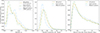 |
Fig. 1. Physical properties of the SGA galaxies used in this study. There are a total of 51 472 galaxies (32 517 spiral galaxies and 18 955 elliptical galaxies). The left panel illustrates the (differential) redshift distribution for all galaxies (orange), spiral galaxies (dotted green) and elliptical galaxies (dotted blue). The central panel depicts the absolute magnitude (R-band) distribution of these galaxies and the right panel illustrates the distribution of galaxy distances from the nearest filament axis (in megaparsecs). |
3. Methodology
3.1. Obtaining spin normal for galaxies
The SGA provides the right ascension (RA), equatorial declination (Dec), magnitude, redshift, axial ratio (b/a), and PA of each galaxy either measured based on second moments of the galaxy’s light distribution or by the TRACTOR model (Lang et al. 2016). Since we are interested in the alignment of a galaxy’s spin axis with filaments, we are faced with three complications. Firstly, galaxy catalogues such as the SGA provide shapes, not spins. Thus, we must use the short axis of a galaxy’s shape as a proxy for its spin. In general, this is a legitimate assumption (and standard practice in the field i.e. Pahwa et al. 2016) since a number of studies have shown that spin vectors align with the short axes of the stellar distribution of rotationally supported disc galaxies as well as for elliptical galaxies (Cappellari et al. 2011; Franx et al. 1991; Krajnović et al. 2011).
The second issue is that we are only able to measure the direction of projected (2D) axes and not the full 3D axis. In order to estimate the inclination angle of spiral galaxies, and thus the 3D short axis direction, we rely on modelling each galaxy’s intrinsic flattening (e.g. see Haynes & Giovanelli 1984; Lee & Erdogdu 2007). Accordingly, the model essentially returns the inclination angle, given the projected short-to-long axis ratio and intrinsic morphology-dependent flattening. Haynes & Giovanelli (1984) provided a catalogue of intrinsic flattening parameters based on their morphology for all subcategories of spiral galaxies, with which the inclination angles were calculated. This inclination is used to de-project the galaxies’ normals and results in a 3D vector that can be used to compute an angle with the 3D filament spine direction.
Since we are looking at 3D angles, these are shown in terms of cosine. It is important to mention that when confronted with an elliptical isophote representing an inclined spiral galaxy, there are two possible inclination angles for a specific spiral galaxy (corresponding to which side of the isophote is closer to the observer). Since there is no (practical) way to break this degeneracy, in this analysis we simply (artificially) double the sample size by including both inclination angles for each spiral. This doubling of the sample size both dilutes the signal and boosts the significance of any signal (by increasing the sample size). These two effects effectively cancel each other out, as is common practice (see Pahwa et al. 2016; Varela et al. 2012; Kashikawa & Okamura 1992).
In the case of elliptical galaxies, the inclination angle is assumed to be 90° (i.e, projected short axis and the spin axis are parallel) as it has been used in previous such studies (Pahwa et al. 2016). Lastly, we note that the ‘handedness’ of a galaxy’s spin is unobtainable, since all that is able to be measured is the axis of the galaxy’s spin axis.
When measuring the alignment between galaxy spin and filament in observational data, we have to be aware of potential biases in the observed data. Both the estimated galaxy spin vector and filament orientation are not uniform with respect to the line of sight. The measured galaxy spin vector is not uniform due to the difficulties of estimating the inclination angle of galaxies. Galaxy filaments are not uniformly distributed due to the redshift space distortions. In Fig. 2 we show the distribution of measured spin axes and galaxy filaments with respect to the line of sight. Due to the combination of these biases, there will be a measured alignment signal between filaments and galaxy spins even if there is a lack of an intrinsic alignment between them. In our statistical analysis (see Sect. 3.2), we take this observational bias into account.
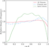 |
Fig. 2. Distribution of the absolute magnitude of the cosine of the angle between the line of sight (l.o.s.) and various objects. In dashed green we show the angle between the l.o.s. and spiral galaxy spin normal. In dash-dotted blue we show the angle between the l.o.s. and the filament spines used (namely those filaments with galaxies in the SGA). In solid red we show the angle between the l.o.s. and all the filament points from the Bisous process (see Tempel et al. 2016b). |
3.2. Estimation of the significance of the alignment signal
The alignment signal was measured by taking the dot product between the galaxy’s implied spin axis and the filament spine (cosine of the angle between the galaxy’s spin vectors and the local filament orientation) and constructing a probability distribution function (PDF). The resultant distribution was then expressed as a kernel density estimation (KDE) and was tested against the null hypothesis of no (random) alignment.
Considering the ambiguity associated with the direction of the spin, i.e. the handedness of the galaxy spin, we used the absolute value of the dot product in constructing the PDF. This has a tendency to weaken any intrinsic signal we find, but the alignment signal that has been obtained here can thus be interpreted as a lower limit, whereas the actual signal could be stronger than this.
All measured signals must be compared to the null hypothesis of a random distribution of angles. Due to implicit biases in observational samples, a random distribution does not necessarily imply a uniform distribution centred around unity (Tempel et al. 2013). As such, the null hypothesis was estimated in the following manner:
A randomized control sample was produced by randomizing each galaxy’s PA in the sky, keeping all other properties unchanged. For each randomized sample, a probability distribution of the cosine of the angle between the galaxy’s (new, randomized) spin axis and the filament spine to which it is assigned was obtained. This process was repeated 10 000 times. The measured alignment signal can then be compared with the random distributions in two ways.
1) The full distribution can be compared. Here we essentially took the mean difference between the measured signal and the median of the 10 000 randoms and expressed this in terms of the standard deviation of the random sample.
2) The mean of the measured signal can be compared with the ‘median of the medians’ of the random sample. In other words, each of the 10 000 random distributions has a median angle. This set of random medians itself has a mean value and a standard deviation. The median of the measured signal can then be compared to the mean of the medians of the random values and again expressed in terms of the standard deviation of this distribution.
3) Lastly, a Kolmogorov–Smirnov (KS) test can be applied to ascertain the KS probability that two distributions are drawn from the same parent distribution. Here we applied the KS test to the measured signal and the randoms to see if their cumulative distribution functions were consistent with each other and, if so, at what level of significance. The key advantage of the KS test is its sensitivity to differences in the entire shape of distributions, making it effective at detecting subtle yet systematic deviations. We note that these three methods have been utilized in numerous studies in this subfield (e.g. Tempel & Libeskind 2013; Pahwa et al. 2016).
Statistical analysis of galaxy-filament alignment signals for spirals and ellipticals within various proximity selections from the filament spine.
4. Results
In Fig. 3 we show the alignment for spiral (left) and elliptical (right) galaxies located within 2 Mpc of the filament spine. The upper row shows the probability distributions (solid line) and the result of the randomization procedure described above. The 1 and 2σ null hypothesis corridor is indicated by the dark and the light cyan bands. The reader will note that the randomization procedure does not produce a uniform band but rather imprints an alignment bias on the sample. The bottom rows of Fig. 3 show the exact same information but now normalized such that the randomization presents as uniform. Throughout the rest of the paper, we display the alignment results in this way, the top row of Fig. 3 being presented for didactical reasons. Two immediate results of this plot stand out:
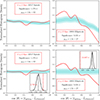 |
Fig. 3. Normalized histogram of cosines of the angles between spines of the filaments and the spin axes of spiral and elliptical galaxies within 2 Mpc ( |

1) Elliptical galaxies (right column) show a statistically significant perpendicular alignment between their short axes ( ) and the filament spine (
 ). Alternatively put: their long axes align with the filament spine. It is detected at the ∼3.6σ level significance from the null hypothesis, and the mean of the alignment signal shows a ∼13σ level significance from the distribution of the mean from the null hypothesis cases.
2) Only a statistically weak alignment (∼1.2σ) is seen when examining the full distribution of spiral galaxy angles. However, the mean angle of the distribution is ∼2.8σ inconsistent with the null hypothesis expectation. This is intriguing since 2.8σ (99.47% inconsistent with random) is approaching the threshold (3σ) that most scientists would consider to be a statistically significant signal.
Taken together, Fig. 3 indicates that using the largest, most modern atlas of galaxy PAs and morphologies, together with the most expansive catalogue of filaments, reaffirms the alignment between elliptical galaxies and the cosmic web and hints at a signal that is up to 99.5% inconsistent with random for spirals. As a natural progression, we extended our analysis to observe the alignment trend as a function of: 1) distance between the galaxies and the spine of their host filament, and 2) absolute magnitude. Lastly, we also ran a machine learning algorithm to isolate the properties that maximize the alignment signal, explained in Section 4.3.
4.1. Alignment signal as a function of filament proximity
The alignment signal was examined as a function of distance from the filament spine across four discrete bins within 2 Mpc to see if any distance dominates the signal. The distances considered here were selected so as to compromise between having (roughly) the same number of galaxies per distance bin and physically relevant distance scales. Figs. 4 and 5 show how the alignment signal of the spiral and elliptical (respectively) depend on distance in both a cumulative (dashed) and differential (solid) fashion.
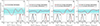 |
Fig. 4. Alignment signal – probability density distribution (PDF) of the cosines of the angle between spines of the filaments and the spin axes of spiral galaxies at different intervals of (< 0.2 Mpc), (0.2–0.5 Mpc), (0.5–1 Mpc), and (1–2 Mpc, in red). The dark cyan band shows the 1σ null hypothesis corridor beyond which the PDF is considered significant. The 2σ band (light cyan) is also provided as a visual comparison for the significance of the PDF. For comparison, the cumulative version for the distance bins (i.e. PDF for all the spiral galaxies that are within the distance range of the upper bound of the distance bin) is superimposed (in dashed blue lines) over the PDF for a given distance interval bin along with their error corridors (in dash-dotted blue lines). Inset plots depicting the mean of the alignment signal (red line: for differential subsets and blue line: for cumulative subsets) along with the distribution of the mean from the null hypothesis cases are inserted to visualize how much further the mean of the alignment signal is from the median of the distribution of the mean from the null hypothesis cases (black line), in terms of the standard deviation of the distribution. The statistical significance of the alignment in each subset is quantified and presented in Table 1 (Note: the alignment signal are normalized with the mean random signal so that the distributions are based around 1.0 for better inference of the alignment signal, and not under the assumption of null hypothesis to be an uniform distribution (refer Fig. 3)). |
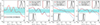 |
Fig. 5. Alignment signal – probability density distribution (PDF) of the cosines of the angle between spines of the filaments and the spin axes of elliptical galaxies at different intervals of (< 0.2 Mpc), (0.2–0.5 Mpc), (0.5–1 Mpc), and (1–2 Mpc). The dark cyan band shows the 1σ null hypothesis corridor beyond which the PDF is considered significant. The 2σ band (light cyan) is also provided as a visual comparison for the significance of the PDF. For comparison, the cumulative version for the distance bins (i.e. PDF for all the elliptical galaxies that are within the distance range of the upper bound of the distance bin) is superimposed (in dashed blue lines) over the PDF for a given distance interval bin along with their error corridors (in dash-dotted blue lines). Inset plots depicting the mean of the alignment signal (red line: for differential subsets and blue line: for cumulative subsets) along with the distribution of the mean from the null hypothesis cases is inserted to visualize how much further the mean of the alignment signal is from the median of the distribution of the mean from the null hypothesis cases (black line), in terms of the standard deviation of the distribution. The statistical significance of the alignment in each subset is quantified and presented in Table 1 (Note: the alignment signal are normalized with the mean random signal so that the distributions are based around 1.0 for better inference of the alignment signal, and not under the assumption of null hypothesis to be an uniform distribution (refer Fig. 3)). |
Table 1 presents the statistical analysis of galaxy-filament alignment for spiral and elliptical galaxies respectively. The table summarizes the following metrics: mean of alignment signal (⟨cosθ⟩), significance from mean of alignment signal (σ⟨cosθ⟩), alignment signal significance (⟨σ⟩), and the KS test p value (pKS) for different proximity selections.
We first turn to Fig. 4, the alignment of spiral galaxies with filaments. Here, the results are unambiguous. At no filamentary distance is the full distribution of the galaxies significantly aligned with the cosmic web in terms of the alignment signal significance (⟨σ⟩). The cumulative distributions (dashed blue lines) are well within their (lighter dash-dotted blue lines) error corridors, as are the solid lines. From Table 1, the significance of alignments are all either well under or slightly above 1 sigma.
The mean of the alignment signal (cos θ) for both the cumulative and the differential subsets are also centred around 0.5, hinting that the disc galaxies used in this analysis do not show a significant alignment trend, irrespective of their proximity (as is also supported by negligible values of pKS). We note that there is a small exception – in the 0.5 < d < 1.0 Mpc and 1.0 < d < 2.0 Mpc range, the roughly 9000 and 10 000 spirals in each distance bracket have a mean angle that is 1.9σ and 2.3σ inconsistent with random. Although the full distributions remain consistent with random at the ∼1σ level, it is noteworthy that the mean behaves somewhat atypically.
In Fig. 5 the alignment for ellipticals is shown, also as a function of filamentary distance. Here, the plots indicate that in the inner core of the filament the alignment is inconsistent with random at a mere 1.2σ level. Beyond 0.2 Mpc, more significant alignments emerge. The differential (solid) lines indicate a mixed picture with statistically significant alignments peaking at the 0.2–0.5 Mpc cylindrical annulus (2.42σ), slightly decreasing in the 0.5–1 Mpc range (1.8σ) and then rising again on the outskirts (1.9σ).
The cumulative (solid) lines maintain a consistent trend of increasing significance, as more galaxies are included. Table 1 also shows that other significance indicators show consistent trends with alignment signal significance (⟨σ⟩) that the alignment is statistically significant for the subset of elliptical galaxies between 0.2–0.5 Mpc from the spine of the filament. Contrary to spirals, the ⟨cosθ⟩ values for each subset of elliptical galaxies from Table 1 are consistently smaller than the median of the distribution of the mean from the null hypothesis case (see inset of Fig. 5) indicating further that the ellipticals indeed have a preferred orientation (namely perpendicular to the filament spine) as a function of proximity to the filament, which is confirmed by larger σ⟨cosθ⟩ significance and significant pKS values (Table 1).
4.2. Alignment signal as a function of absolute luminosity
Statistical analysis of galaxy-filament alignment signals for spiral and elliptical galaxies within various absolute luminosity (M) ranges.
We attempted to study the alignment signal as a function of brightness, since theoretical studies such as Lee (2004) found that brighter spiral galaxies had a more pronounced alignment with the filaments compared to their lesser luminous counterparts. Here, in this study, we have performed our analysis as a function of absolute luminosity in the R band for both spiral and elliptical galaxies.
Figs. 6 and 7 show the alignment trend for both spiral and elliptical galaxies across four luminosity bins, each containing ∼8130 spirals and ∼4739 ellipticals, respectively. For spirals (Fig. 6, Table 2), none of the subsets exhibit a strong alignment. The most pronounced signal, in terms of significance (⟨σ⟩) occurs in the third bin (−21.48 ≤ M < −20.76), in which the mean alignment strength rises to 1.263σ above the randomized expectation, with a pKS value of 2.3 × 10⁻².
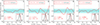 |
Fig. 6. Normalized histogram of the alignment between spiral galaxy spins and cosmic filaments, based on different luminosity bins. Each panel represents the distribution of the alignment signal (cos (θ)) for spiral galaxies with absolute magnitudes in the following ranges: (a) −19.86 ≤ M (b) −20.76 ≤ M ≤ −19.86 (c) −21.48 ≤ M ≤ −20.76, and d) M ≤ −21.48. The alignment is quantified as the cosine of the angle between the galaxy spin vector and the filament axis. An inset plot depicting the mean of the alignment signal (red line) along with the distribution of the mean from the null hypothesis cases is inserted to visualize how much further the mean of the alignment signal is from the median of the distribution of the mean from the null hypothesis cases (black line), in terms of the standard deviation of the distribution. The statistical significance of alignment in each subset is quantified and presented in Table 2 (Note: the alignment signals are normalized with the mean random signal so that the distributions are based around 1.0 for better inference of the alignment signal, and not under the assumption of null hypothesis to be an uniform distribution (refer Fig. 3)). |
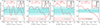 |
Fig. 7. Normalized histogram of the alignment between elliptical galaxy spins and cosmic filaments, based on different luminosity bins. Each panel represents the distribution of the alignment signal (cos (θ)) for elliptical galaxies with absolute magnitudes in the following ranges: (a) −20.98 ≤ M (b) −21.68 ≤ M ≤ −20.98 (c) −22.20 ≤ M ≤ −21.68, and d) M ≤ −22.20. The alignment is quantified as the cosine of the angle between the galaxy spin vector and the filament axis. An inset plot depicting the mean of the alignment signal (red line) along with the distribution of the mean from the null hypothesis cases is inserted to visualize how much further the mean of the alignment signal is from the median of the distribution of the mean from the null hypothesis cases (black line), in terms of the standard deviation of the distribution. The statistical significance of alignment in each subset is quantified and presented in Table 2 (Note: the alignment signals are normalized with the mean random signal so that the distributions are based around 1.0 for better inference of the alignment signal, and not under the assumption of null hypothesis to be an uniform distribution (refer Fig. 3)). |
However, even here the absolute cosine ⟨cosθ⟩≃0.500 remains essentially indistinguishable from random, matching well with the visual inspection of the alignment signal, which appears to be random. On the other hand, the brightest disc galaxies show an alignment trend and are additionally supported by a comparatively higher σ⟨cosθ⟩, again has a ⟨cosθ⟩≃0.500, indicating a very weak alignment trend (also inferred from their respective pKS and ⟨σ⟩ values).
By contrast, ellipticals (Fig. 7, and again Table 2) display a steadily strengthening perpendicular alignment as one moves to brighter bins. The faintest ellipticals (M ≥ −20.99) already show a marginal 1.393σ significance (pKS = 3.6 × 10⁻²), but this rises to 1.471σ (pKS = 9.1 × 10⁻⁷) for −21.69 ≤ M < −20.99, and to 2.092 σ (pKS = 4.6 × 10⁻⁸) for −22.20 ≤ M < −21.69, peaking at 3.107σ (pKS = 9.7 × 10⁻¹⁸) for the brightest ellipticals (M < −22.20).
Thus, massive ellipticals exhibit the strongest and most significant perpendicular alignment with the filamentary network, whereas spiral discs show no analogous luminosity trend.
4.3. Obtaining the subset with maximum significance
Observational studies have consistently shown that recovering an alignment signal with spirals is only possible under stringent sub-sample cuts; for example, selecting bright spirals (Tempel et al. 2013), pure disc or low-bulge-fraction systems (Barsanti et al. 2022), high-spin late types (fast rotators) (Kraljic et al. 2021), or edge-on discs (Jones et al. 2010). To further refine our sensitivity to the notoriously weak spiral–filament alignment and to see if there is a specific subset with maximum statistical significance, we implemented a Bayesian optimization involving the two factors we performed our study on: the absolute r-band magnitude and the projected filament distance.
Statistical analysis of sub-sample from spiral and elliptical galaxies as function of proximity and luminosity with significant alignment.
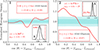 |
Fig. 8. Normalized histogram of cosines of the angles between spines of the filaments and the spin axes of subset of spiral and elliptical galaxies with maximum significance. ( |

We employed a Gaussian process (GP)–based Bayesian optimization method (using the gp_minimize routine from SCIKIT-OPTIMIZE). This approach constructs a probabilistic surrogate model of the objective function to efficiently explore a 4D parameter space – defined by the minimum and maximum absolute r-band magnitudes ( ) and the minimum and maximum projected filament distances (
 ) – without requiring an exhaustive grid search.
We performed the optimization separately for the spiral and elliptical samples, allowing each morphological class to have distinct optimal criteria. For spirals, the algorithm converged on subsets of relatively bright disc galaxies at intermediate-to-large filament distances (approximately −23.5 ≤ Mr ≤ −16.0 and 0.36 ≤ d ≤ 2.00 Mpc), whereas for ellipticals the highest significance was achieved by focusing on the brightest ellipticals (Mr ≲ −20.7) over the full distance range (d ≤ 2.0 Mpc). The Bayesian optimizer inherently penalizes overly restrictive cuts that yield insufficient sample sizes by returning low objective values when the subset size falls below the reliability threshold, ensuring that the resulting subsets both maximize the alignment signal and retain adequate statistical robustness. Even after this targeted selection, spiral alignments remain marginal.
Fig. 8 provides the alignment trend for the subset of early type and disc galaxies with maximum statistical significance. Table 3 summarizes the respective statistical metrics for these subsets. Even after this targeted selection, the spiral subset attains only a marginal ∼1.6σ signal, consistent with previous findings that broadly defined spiral samples mask the expected parallel alignment unless one isolates the most disc-dominated, well-inclined galaxies (e.g. Hirv et al. 2017; Pahwa et al. 2016). (∼1.6σ), while ellipticals exhibit a robust ∼3.8σ perpendicular alignment. Note that when the mean value is examined, the spirals are 3.8σ away from random and the ellipticals 13.8σ events. This application of Bayesian optimization therefore pinpoints the luminosity and environmental regimes within the galaxy catalogue in which the cosmic spin–filament alignment is most pronounced.
5. Summary and conclusion
In this paper we have examined the alignment between spiral and elliptical galaxies and the cosmic network of filaments. A large body of work has been published dedicated to examining such an alignment: whether it is to understand the origin of angular momentum (Schäfer 2009) or intrinsic alignments as a nuisance parameter in lensing surveys (Amon et al. 2022), the positioning of galaxies is a well-studied phenomenon in observations as well as simulations. Here we repeat previous studies, but with the largest sample of elliptical and spiral galaxies to date.
A number of challenges – or partially arbitrary choices – exist that influence the detection of a potential signal. The first set of questions concerns the method of quantifying the LSSs (e.g. Libeskind et al. (2017)). Here we opt for a fairly straightforward method, the point process known as the Bisous method, whose direction has been shown to be consistent with, if not all, at least two methods – the V and T web, Hoffman et al. (2012) and Hahn et al. (2010) respectively (see Libeskind et al. 2015). The identification of the LSS is not as ambiguous or degenerate as to cause major concern; however, it is a source of some uncertainty.
More critical is the determination of the spin axis of a galaxy. As written above, we must transform a projected ellipse into a 3D ellipsoid. Multiple degeneracies exist that all serve to wipe out an intrinsic signal among them, the handedness and the line of sight degeneracy; namely, if an axis is pointing towards or away from the observer at some inclination angle. While employing galaxy modelling as performed here (e.g. Lee & Erdogdu 2007) helps to strengthen any potential signal, is clearly a small step in the right direction. Determining the true 3D short axis of a galaxy remains the greatest unknown in works such as this.
Given all the issues mentioned above, it is remarkable that any signal persists. Ellipticals exhibit a strong perpendicular alignment: in the optimal bin (0 ≤ d ≤ 2 Mpc, −24 ≤ M ≤ −20.7) we measure ⟨σ⟩ = 3.772σ, σ⟨cosθ⟩ = 13.792σ and the pKS = 6.6 × 10⁻²⁸, consistent with both earlier observations (e.g. Tempel & Libeskind 2013) and hydrodynamical simulations of massive, pressure-supported galaxies (e.g. Codis et al. 2018; Kraljic et al. 2020). The slight variation in signal strength with filament proximity may reflect filament boundary effects (Wang et al. 2020).
Spirals, by contrast, show no alignment in the full SGA sample, but a targeted selection (0.36 ≤ d ≤ 2 Mpc, −23.46 ≤ M ≤ −16) reveals a faint parallel signal when the full distribution is considered (⟨σ⟩ = 1.567σ) but a stronger signal when examining the median of the distribution (σ⟨cosθ⟩ = 3.859σ and the pKS = 6.6 × 10⁻²⁸, Fig. 8, Table 3). This echoes recent results from MaNGA (Kraljic et al. 2021), the SIMBA simulation (Kraljic et al. 2020), and the CHILES/Blue Bird HI survey (Blue Bird et al. 2020), all of which report low-mass systems’ spins parallel to filaments, which is a trend also observed in early studies (e.g. Tempel & Libeskind 2013; Codis et al. 2018)
A note is in order regarding the difference between the statistical significances found when comparing the full distribution and the median values to random samples. It may be counterintuitive that these metrics disagree. Yet, the reader may consider the following. The median value is not sensitive to individual outliers, but is sensitive to groups of outliers. While the full distribution of the measured signal may well lie within the variance of the random distributions, its median is far more sensitive to outlying values. Ultimately, we only have one measured median, and we are comparing this to 10 000 random medians. The standard deviation of these 10 000 random medians probes the likelihood that one would obtain as many outliers as the signal. This is shown to be a far more sensitive metric than comparing the full distributions – and we note that a sensitive metric is precisely what is needed when trying to suss out a weak signal, buried in statistical noise, and compromised by inclination and shape degeneracies.
The faintness of the SGA spiral signal likely stems from the aforementioned effects (inclination, degeneracies, etc.), and on the other hand, it could also be possible misalignment between stellar discs and their host dark halos (e.g. Welker et al. 2020). More studies (specifically assessing the spin direction of satellites within a host) could shed light on the faint alignment detection with spirals and also enable us to pin down the selection criteria that would give us the subset of disc galaxies with a profound alignment signal and understand the principle behind it.
In the coming years, new observational data will allow us to study the intrinsic connection between galaxies and the cosmic web with great detail. Some of the most promising surveys are the 4MOST (de Jong et al. 2019), WAVES (Driver et al. 2019) and 4HS (Taylor et al. 2023) surveys that will map the cosmic web in the nearby Universe (z < 0.2) with great detail down to the megaparsec scale, allowing us to see the small filaments and tendrils that influence the alignment of galaxies in the cosmic web.
Acknowledgments
We acknowledge the funding from the European Union’s Horizon Europe research and innovation programme (EXCOSM, grant No. 101159513). ET was funded by the Estonian Ministry of Education and Research (grant TK202), Estonian Research Council (grant PRG1006).
References
- Alam, S., Albareti, F. D., Allende Prieto, C., et al. 2015, ApJS, 219, 12 [Google Scholar]
- Amon, A., Gruen, D., Troxel, M. A., et al. 2022, Phys. Rev. D, 105, 023514 [NASA ADS] [CrossRef] [Google Scholar]
- Antipova, A. V., Makarov, D. I., Libeskind, N. I., & Tempel, E. 2025, PASA, 42, e084 [Google Scholar]
- Aragón-Calvo, M. A., van de Weygaert, R., Jones, B. J. T., & van der Hulst, J. M. 2007, ApJ, 655, L5 [Google Scholar]
- Aragon-Calvo, M. A., & Yang, L. F. 2014, MNRAS, 440, L46 [NASA ADS] [CrossRef] [Google Scholar]
- Barnes, J., & Efstathiou, G. 1987, ApJ, 319, 575 [NASA ADS] [CrossRef] [Google Scholar]
- Barsanti, S., Owers, M. S., Brough, S., et al. 2018, ApJ, 857, 71 [NASA ADS] [CrossRef] [Google Scholar]
- Barsanti, S., Colless, M., Welker, C., et al. 2022, MNRAS, 516, 3569 [NASA ADS] [CrossRef] [Google Scholar]
- Binggeli, B. 1982, A&A, 107, 338 [NASA ADS] [Google Scholar]
- Blue Bird, J., Davis, J., Luber, N., et al. 2020, MNRAS, 492, 153 [NASA ADS] [CrossRef] [Google Scholar]
- Bond, J. R., Kofman, L., & Pogosyan, D. 1996, Nature, 380, 603 [NASA ADS] [CrossRef] [Google Scholar]
- Brunino, R., Trujillo, I., Pearce, F. R., & Thomas, P. A. 2007, MNRAS, 375, 184 [Google Scholar]
- Cabanela, J. E., & Aldering, G. 1998, AJ, 116, 1094 [Google Scholar]
- Cappellari, M., Emsellem, E., Krajnović, D., et al. 2011, MNRAS, 416, 1680 [Google Scholar]
- Catinella, B., Schiminovich, D., Cortese, L., et al. 2013, MNRAS, 436, 34 [NASA ADS] [CrossRef] [Google Scholar]
- Codis, S., Pichon, C., Devriendt, J., et al. 2012, MNRAS, 427, 3320 [NASA ADS] [CrossRef] [Google Scholar]
- Codis, S., Pichon, C., & Pogosyan, D. 2015, MNRAS, 452, 3369 [Google Scholar]
- Codis, S., Jindal, A., Chisari, N. E., et al. 2018, MNRAS, 481, 4753 [Google Scholar]
- Cooke, K. C., Kartaltepe, J. S., Rose, C., et al. 2023, ApJ, 942, 49 [NASA ADS] [CrossRef] [Google Scholar]
- de Jong, R. S., Agertz, O., Berbel, A. A., et al. 2019, The Messenger, 175, 3 [NASA ADS] [Google Scholar]
- de Vaucouleurs, G., de Vaucouleurs, A., Corwin, Jr., H. G., et al. 1991, Third Reference Catalogue of Bright Galaxies [Google Scholar]
- Dressler, A. 1980, ApJ, 236, 351 [Google Scholar]
- Driver, S. P., Liske, J., Davies, L. J. M., et al. 2019, The Messenger, 175, 46 [NASA ADS] [Google Scholar]
- Dubois, Y., Pichon, C., Welker, C., et al. 2014, MNRAS, 444, 1453 [Google Scholar]
- Forero-Romero, J. E., Contreras, S., & Padilla, N. 2014, MNRAS, 443, 1090 [NASA ADS] [CrossRef] [Google Scholar]
- Franx, M., Illingworth, G., & de Zeeuw, T. 1991, ApJ, 383, 112 [CrossRef] [Google Scholar]
- Ganeshaiah Veena, P., Cautun, M., van de Weygaert, R., et al. 2018, MNRAS, 481, 414 [NASA ADS] [CrossRef] [Google Scholar]
- Ganeshaiah Veena, P., Cautun, M., Tempel, E., van de Weygaert, R., & Frenk, C. S. 2019, MNRAS, 487, 1607 [NASA ADS] [CrossRef] [Google Scholar]
- Guo, Q., Tempel, E., & Libeskind, N. I. 2015, ApJ, 800, 112 [Google Scholar]
- Hahn, O., Carollo, C. M., Porciani, C., & Dekel, A. 2007, MNRAS, 381, 41 [NASA ADS] [CrossRef] [Google Scholar]
- Hahn, O., Teyssier, R., & Carollo, C. M. 2010, MNRAS, 405, 274 [NASA ADS] [Google Scholar]
- Haynes, M. P., & Giovanelli, R. 1984, AJ, 89, 758 [Google Scholar]
- Hirv, A., Pelt, J., Saar, E., et al. 2017, A&A, 599, A31 [NASA ADS] [CrossRef] [EDP Sciences] [Google Scholar]
- Hoffman, Y., Metuki, O., Yepes, G., et al. 2012, MNRAS, 425, 2049 [Google Scholar]
- Hogg, D. W., Blanton, M. R., Brinchmann, J., et al. 2004, ApJ, 601, L29 [NASA ADS] [CrossRef] [Google Scholar]
- Holmberg, E. 1969, Arkiv for Astronomi, 5, 305 [Google Scholar]
- Hoyle, F. 1949, MNRAS, 109, 365 [Google Scholar]
- Huchra, J. P., Macri, L. M., Masters, K. L., et al. 2012, ApJS, 199, 26 [Google Scholar]
- Jõeveer, M., Einasto, J., & Tago, E. 1978, MNRAS, 185, 357 [Google Scholar]
- Jones, B. J. T., van de Weygaert, R., & Aragón-Calvo, M. A. 2010, MNRAS, 408, 897 [NASA ADS] [CrossRef] [Google Scholar]
- Kashikawa, N., & Okamura, S. 1992, PASJ, 44, 493 [NASA ADS] [Google Scholar]
- Kauffmann, G., White, S. D. M., Heckman, T. M., et al. 2004, MNRAS, 353, 713 [Google Scholar]
- Krajnović, D., Emsellem, E., Cappellari, M., et al. 2011, MNRAS, 414, 2923 [Google Scholar]
- Kraljic, K., Davé, R., & Pichon, C. 2020, MNRAS, 493, 362 [NASA ADS] [CrossRef] [Google Scholar]
- Kraljic, K., Duckworth, C., Tojeiro, R., et al. 2021, MNRAS, 504, 4626 [NASA ADS] [CrossRef] [Google Scholar]
- Krolewski, A., Ho, S., Chen, Y.-C., et al. 2019, ApJ, 876, 52 [NASA ADS] [CrossRef] [Google Scholar]
- Kuutma, T., Tamm, A., & Tempel, E. 2017, A&A, 600, L6 [NASA ADS] [CrossRef] [EDP Sciences] [Google Scholar]
- Laigle, C., Pichon, C., Codis, S., et al. 2014, MNRAS, 446, 2744 [Google Scholar]
- Lang, D., Hogg, D. W., & Mykytyn, D. 2016, Astrophysics Source Code Library [record ascl:1604.008] [Google Scholar]
- Lee, J. 2004, ApJ, 614, L1 [NASA ADS] [CrossRef] [Google Scholar]
- Lee, J., & Erdogdu, P. 2007, ApJ, 671, 1248 [Google Scholar]
- Lee, J., & Pen, U.-L. 2002, ApJ, 567, L111 [NASA ADS] [CrossRef] [Google Scholar]
- Libeskind, N. I., Hoffman, Y., Knebe, A., et al. 2012, MNRAS, 421, L137 [NASA ADS] [CrossRef] [Google Scholar]
- Libeskind, N. I., Hoffman, Y., Forero-Romero, J., et al. 2013a, MNRAS, 428, 2489 [NASA ADS] [CrossRef] [Google Scholar]
- Libeskind, N. I., Hoffman, Y., Steinmetz, M., et al. 2013b, ApJ, 766, L15 [Google Scholar]
- Libeskind, N. I., Knebe, A., Hoffman, Y., & Gottlöber, S. 2014, MNRAS, 443, 1274 [NASA ADS] [CrossRef] [Google Scholar]
- Libeskind, N. I., Tempel, E., Hoffman, Y., Tully, R. B., & Courtois, H. 2015, MNRAS, 453, L108 [Google Scholar]
- Libeskind, N. I., van de Weygaert, R., Cautun, M., et al. 2017, MNRAS, 473, 1195 [Google Scholar]
- Makarov, P. P., Terekhova, N., Courtois, H., & Vauglin, I. 2014, A&A, 570, A13 [NASA ADS] [CrossRef] [EDP Sciences] [Google Scholar]
- Moustakas, J., Lang, D., Dey, A., et al. 2023, ApJS, 269, 3 [NASA ADS] [CrossRef] [Google Scholar]
- Navarro, J. F., Abadi, M. G., & Steinmetz, M. 2004, ApJ, 613, L41 [NASA ADS] [CrossRef] [Google Scholar]
- Pahwa, I., Libeskind, N. I., Tempel, E., et al. 2016, MNRAS, 457, 695 [NASA ADS] [CrossRef] [Google Scholar]
- Peebles, P. J. E. 1969, ApJ, 155, 393 [Google Scholar]
- Peng, Y.-J., & Maiolino, R. 2013, MNRAS, 438, 262 [Google Scholar]
- Pichon, C., Codis, S., & Pogosyan, D. 2016, in The Zeldovich Universe: Genesis and Growth of the Cosmic Web, eds. R. van de Weygaert, S. Shandarin, E. Saar, & J. Einasto, IAU Symp., 308, 421 [Google Scholar]
- Porciani, C., Dekel, A., & Hoffman, Y. 2002, MNRAS, 332, 325 [NASA ADS] [CrossRef] [Google Scholar]
- Schäfer, B. M. 2009, Int. J. Mod. Phys. D, 18, 173 [Google Scholar]
- Stoica, R. S., Martínez, V. J., & Saar, E. 2007, J. Royal Statist. Soc. Ser. C: Appl. Statist., 56, 459 [Google Scholar]
- Stoica, R. S., Martínez, V. J., & Saar, E. 2010, A&A, 510, A38 [CrossRef] [EDP Sciences] [Google Scholar]
- Taylor, E. N., Cluver, M., Bell, E., et al. 2023, The Messenger, 190, 46 [NASA ADS] [Google Scholar]
- Tempel, E., & Libeskind, N. I. 2013, ApJ, 775, L42 [NASA ADS] [CrossRef] [Google Scholar]
- Tempel, E., Stoica, R. S., & Saar, E. 2013, MNRAS, 428, 1827 [NASA ADS] [CrossRef] [Google Scholar]
- Tempel, E., Libeskind, N. I., Hoffman, Y., Liivamägi, L. J., & Tamm, A. 2014a, MNRAS, 437, L11 [Google Scholar]
- Tempel, E., Stoica, R. S., Martínez, V. J., et al. 2014b, MNRAS, 438, 3465 [CrossRef] [Google Scholar]
- Tempel, E., Guo, Q., Kipper, R., & Libeskind, N. I. 2015, MNRAS, 450, 2727 [NASA ADS] [CrossRef] [Google Scholar]
- Tempel, E., Kipper, R., Tamm, A., et al. 2016a, A&A, 588, A14 [NASA ADS] [CrossRef] [EDP Sciences] [Google Scholar]
- Tempel, E., Stoica, R. S., Kipper, R., & Saar, E. 2016b, Astron. Comput., 16, 17 [NASA ADS] [CrossRef] [Google Scholar]
- Tempel, E., Tuvikene, T., Kipper, R., & Libeskind, N. I. 2017, A&A, 602, A100 [NASA ADS] [CrossRef] [EDP Sciences] [Google Scholar]
- Trowland, H. E., Lewis, G. F., & Bland-Hawthorn, J. 2013, ApJ, 762, 72 [CrossRef] [Google Scholar]
- Trujillo, I., Carretero, C., & Patiri, S. G. 2006, ApJ, 640, L111 [NASA ADS] [CrossRef] [Google Scholar]
- Varela, J., Betancort-Rijo, J., Trujillo, I., & Ricciardelli, E. 2012, ApJ, 744, 82 [NASA ADS] [CrossRef] [Google Scholar]
- Wang, P., & Kang, X. 2017, MNRAS, 468, L123 [NASA ADS] [CrossRef] [Google Scholar]
- Wang, P., & Kang, X. 2018, MNRAS, 473, 1562 [Google Scholar]
- Wang, P., Guo, Q., Kang, X., & Libeskind, N. I. 2018, ApJ, 866, 138 [NASA ADS] [CrossRef] [Google Scholar]
- Wang, P., Libeskind, N. I., Tempel, E., et al. 2020, ApJ, 900, 129 [NASA ADS] [CrossRef] [Google Scholar]
- Welker, C., Bland-Hawthorn, J., van de Sande, J., et al. 2020, MNRAS, 491, 2864 [NASA ADS] [CrossRef] [Google Scholar]
- White, S. D. M. 1984, ApJ, 286, 38 [NASA ADS] [CrossRef] [Google Scholar]
- Willett, K. W., Lintott, C. J., Bamford, S. P., et al. 2013, MNRAS, 435, 2835 [Google Scholar]
- York, D. G., Adelman, J., Anderson, J. E., Jr, et al. 2000, AJ, 120, 1579 [Google Scholar]
- Zehavi, I., Zheng, Z., Weinberg, D. H., et al. 2005, ApJ, 630, 1 [Google Scholar]
- Zhang, Y., Yang, X., Faltenbacher, A., et al. 2009, ApJ, 706, 747 [NASA ADS] [CrossRef] [Google Scholar]
- Zhang, Y., Yang, X., Wang, H., et al. 2015, ApJ, 798, 17 [Google Scholar]
All Tables
Statistical analysis of galaxy-filament alignment signals for spirals and ellipticals within various proximity selections from the filament spine.
Statistical analysis of galaxy-filament alignment signals for spiral and elliptical galaxies within various absolute luminosity (M) ranges.
Statistical analysis of sub-sample from spiral and elliptical galaxies as function of proximity and luminosity with significant alignment.
All Figures
|
Fig. 1. Physical properties of the SGA galaxies used in this study. There are a total of 51 472 galaxies (32 517 spiral galaxies and 18 955 elliptical galaxies). The left panel illustrates the (differential) redshift distribution for all galaxies (orange), spiral galaxies (dotted green) and elliptical galaxies (dotted blue). The central panel depicts the absolute magnitude (R-band) distribution of these galaxies and the right panel illustrates the distribution of galaxy distances from the nearest filament axis (in megaparsecs). |
| In the text | |
|
Fig. 2. Distribution of the absolute magnitude of the cosine of the angle between the line of sight (l.o.s.) and various objects. In dashed green we show the angle between the l.o.s. and spiral galaxy spin normal. In dash-dotted blue we show the angle between the l.o.s. and the filament spines used (namely those filaments with galaxies in the SGA). In solid red we show the angle between the l.o.s. and all the filament points from the Bisous process (see Tempel et al. 2016b). |
| In the text | |
|
Fig. 3. Normalized histogram of cosines of the angles between spines of the filaments and the spin axes of spiral and elliptical galaxies within 2 Mpc ( |
| In the text | |
|
Fig. 4. Alignment signal – probability density distribution (PDF) of the cosines of the angle between spines of the filaments and the spin axes of spiral galaxies at different intervals of (< 0.2 Mpc), (0.2–0.5 Mpc), (0.5–1 Mpc), and (1–2 Mpc, in red). The dark cyan band shows the 1σ null hypothesis corridor beyond which the PDF is considered significant. The 2σ band (light cyan) is also provided as a visual comparison for the significance of the PDF. For comparison, the cumulative version for the distance bins (i.e. PDF for all the spiral galaxies that are within the distance range of the upper bound of the distance bin) is superimposed (in dashed blue lines) over the PDF for a given distance interval bin along with their error corridors (in dash-dotted blue lines). Inset plots depicting the mean of the alignment signal (red line: for differential subsets and blue line: for cumulative subsets) along with the distribution of the mean from the null hypothesis cases are inserted to visualize how much further the mean of the alignment signal is from the median of the distribution of the mean from the null hypothesis cases (black line), in terms of the standard deviation of the distribution. The statistical significance of the alignment in each subset is quantified and presented in Table 1 (Note: the alignment signal are normalized with the mean random signal so that the distributions are based around 1.0 for better inference of the alignment signal, and not under the assumption of null hypothesis to be an uniform distribution (refer Fig. 3)). |
| In the text | |
|
Fig. 5. Alignment signal – probability density distribution (PDF) of the cosines of the angle between spines of the filaments and the spin axes of elliptical galaxies at different intervals of (< 0.2 Mpc), (0.2–0.5 Mpc), (0.5–1 Mpc), and (1–2 Mpc). The dark cyan band shows the 1σ null hypothesis corridor beyond which the PDF is considered significant. The 2σ band (light cyan) is also provided as a visual comparison for the significance of the PDF. For comparison, the cumulative version for the distance bins (i.e. PDF for all the elliptical galaxies that are within the distance range of the upper bound of the distance bin) is superimposed (in dashed blue lines) over the PDF for a given distance interval bin along with their error corridors (in dash-dotted blue lines). Inset plots depicting the mean of the alignment signal (red line: for differential subsets and blue line: for cumulative subsets) along with the distribution of the mean from the null hypothesis cases is inserted to visualize how much further the mean of the alignment signal is from the median of the distribution of the mean from the null hypothesis cases (black line), in terms of the standard deviation of the distribution. The statistical significance of the alignment in each subset is quantified and presented in Table 1 (Note: the alignment signal are normalized with the mean random signal so that the distributions are based around 1.0 for better inference of the alignment signal, and not under the assumption of null hypothesis to be an uniform distribution (refer Fig. 3)). |
| In the text | |
|
Fig. 6. Normalized histogram of the alignment between spiral galaxy spins and cosmic filaments, based on different luminosity bins. Each panel represents the distribution of the alignment signal (cos (θ)) for spiral galaxies with absolute magnitudes in the following ranges: (a) −19.86 ≤ M (b) −20.76 ≤ M ≤ −19.86 (c) −21.48 ≤ M ≤ −20.76, and d) M ≤ −21.48. The alignment is quantified as the cosine of the angle between the galaxy spin vector and the filament axis. An inset plot depicting the mean of the alignment signal (red line) along with the distribution of the mean from the null hypothesis cases is inserted to visualize how much further the mean of the alignment signal is from the median of the distribution of the mean from the null hypothesis cases (black line), in terms of the standard deviation of the distribution. The statistical significance of alignment in each subset is quantified and presented in Table 2 (Note: the alignment signals are normalized with the mean random signal so that the distributions are based around 1.0 for better inference of the alignment signal, and not under the assumption of null hypothesis to be an uniform distribution (refer Fig. 3)). |
| In the text | |
|
Fig. 7. Normalized histogram of the alignment between elliptical galaxy spins and cosmic filaments, based on different luminosity bins. Each panel represents the distribution of the alignment signal (cos (θ)) for elliptical galaxies with absolute magnitudes in the following ranges: (a) −20.98 ≤ M (b) −21.68 ≤ M ≤ −20.98 (c) −22.20 ≤ M ≤ −21.68, and d) M ≤ −22.20. The alignment is quantified as the cosine of the angle between the galaxy spin vector and the filament axis. An inset plot depicting the mean of the alignment signal (red line) along with the distribution of the mean from the null hypothesis cases is inserted to visualize how much further the mean of the alignment signal is from the median of the distribution of the mean from the null hypothesis cases (black line), in terms of the standard deviation of the distribution. The statistical significance of alignment in each subset is quantified and presented in Table 2 (Note: the alignment signals are normalized with the mean random signal so that the distributions are based around 1.0 for better inference of the alignment signal, and not under the assumption of null hypothesis to be an uniform distribution (refer Fig. 3)). |
| In the text | |
|
Fig. 8. Normalized histogram of cosines of the angles between spines of the filaments and the spin axes of subset of spiral and elliptical galaxies with maximum significance. ( |
| In the text | |
Current usage metrics show cumulative count of Article Views (full-text article views including HTML views, PDF and ePub downloads, according to the available data) and Abstracts Views on Vision4Press platform.
Data correspond to usage on the plateform after 2015. The current usage metrics is available 48-96 hours after online publication and is updated daily on week days.
Initial download of the metrics may take a while.