| Issue |
A&A
Volume 703, November 2025
|
|
|---|---|---|
| Article Number | A85 | |
| Number of page(s) | 14 | |
| Section | Cosmology (including clusters of galaxies) | |
| DOI | https://doi.org/10.1051/0004-6361/202554248 | |
| Published online | 07 November 2025 | |
The origin of the intracluster light in The Three Hundred simulations
1
Departamento de Física Teórica, Módulo 15, Facultad de Ciencias, Universidad Autónoma de Madrid, 28049 Madrid, Spain
2
Departamento de Astrofísica, Universidad de La Laguna, Av. Astrofísico Francisco Sanchez s/n, 38206 La Laguna, Tenerife, Spain
3
Instituto de Astrofísica de Canarias, C/Vía Láctea s/n, 38205 La Laguna, Tenerife, Spain
4
Centro de Investigación Avanzada en Física Fundamental (CIAFF), Facultad de Ciencias, Universidad Autónoma de Madrid, 28049 Madrid, Spain
5
International Centre for Radio Astronomy Research, University of Western Australia, 35 Stirling Highway, Crawley, Western Australia 6009, Australia
6
Institute for Astronomy, University of Edinburgh, Royal Observatory, Blackford Hill, Edinburgh EH9 3HJ, UK
7
Department of Physics and Astronomy, University of Waterloo, Waterloo, Ontario N2L 3G1, Canada
8
Waterloo Centre for Astrophysics, University of Waterloo, Waterloo, Ontario N2L 3G1, Canada
9
Centre for Astrophysics & Supercomputing, Swinburne University of Technology, 1 Alfred St, Hawthorn, VIC 3122, Australia
10
ARC Centre of Excellence for Dark Matter Particle Physics (CDM), Melbourne, Australia
11
School of Physics & Astronomy, University of Nottingham, Nottingham NG7 2RD, United Kingdom
12
INAF – Osservatorio Astronomico di Trieste, Via Tiepolo 11, I34131 Trieste, Italy
13
IFPU – Institute for Fundamental Physics of the Universe, Via Beirut 2, 34151 Trieste, Italy
14
Department of Physics, University of Michigan, 450 Church St, Ann Arbor, MI 48109, USA
15
Instituto de Astronomía y Física del Espacio (IAFE, CONICET-UBA), CC 67, Suc. 28, 1428 Buenos Aires, Argentina
⋆ Corresponding author: This email address is being protected from spambots. You need JavaScript enabled to view it.
Received:
24
February
2025
Accepted:
17
September
2025
Abstract
We investigated the origin and formation mechanisms of the intracluster light (ICL) in THE THREE HUNDRED simulations, a set of 324 hydrodynamically resimulated massive galaxy clusters. The ICL, a diffuse component comprised of stars not bound to any individual galaxy, serves as a critical tracer of cluster formation and evolution. Using two implementations of hydrodynamics, GADGET-X and GIZMO-SIMBA, we identified the stellar particles that constitute the ICL at z = 0 and traced them back in time to the moments when they were formed and accreted into the ICL. Our analysis reveals that, across our 324 clusters, half of the present-day ICL mass is typically in place between z ∼ 0.2 and 0.5. The main ICL formation channel is the stripping of stars from subhalos after their infall into the host cluster. Within this channel, 65−80% of the ICL comes from objects with stellar (infall) masses above 1011 M⊙, corresponding to massive galaxies, groups and clusters. When we also consider the ratio of the infalling halo to the total cluster mass, we see that a median of 35% of the mass is brought in major merger events, although the percentage varies significantly across clusters (15−55%). Additional contributions come from minor mergers (25−35%) and smooth accretion (20−50%). The infall redshift of the primary contributors is generally below z ≤ 1, with smaller fractions arriving at redshifts between 1 and 2. Regarding other formation channels, we find minor contributions from stars formed in subhalos after their infall and stars stripped while their contributing halo remains outside the host cluster (and can eventually fall inside or stay outside). Finally, for our two sets of simulations, we find medians of 12 (GADGET-X) and 2 (GIZMO-SIMBA) percent of the ICL mass formed in situ, i.e. directly as part of the diffuse component. However, this component can be attributed to stripping of gas in high-velocity infalling satellite galaxies.
Key words: methods: numerical / galaxies: clusters: general / galaxies: halos / cosmology: theory / large-scale structure of Universe
© The Authors 2025
 Open Access article, published by EDP Sciences, under the terms of the Creative Commons Attribution License (https://creativecommons.org/licenses/by/4.0), which permits unrestricted use, distribution, and reproduction in any medium, provided the original work is properly cited.
This article is published in open access under the Subscribe to Open model. This email address is being protected from spambots. You need JavaScript enabled to view it. to support open access publication.
1. Introduction
The intracluster light (ICL) is a diffuse component in galaxy clusters, coming from stars that are not bound to any individual galaxy but to the potential of the cluster itself. It was first theorised and then discovered more than 70 years ago by Zwicky (1937, 1951). However, over the past two decades, interest in the ICL has grown significantly due to the advent of modern instruments that allow us to observe this faint light from galaxy clusters. The formation of the ICL is closely linked to that of the cluster, and so it carries information about the past, present, and future history of the cluster (see e.g. reviews by Contini 2021; Montes 2019, 2022). Thus, understanding the ICL becomes essential for a complete understanding of galaxy clusters and their role in galaxy evolution.
Despite its importance, defining and quantifying the ICL remains a major challenge, both observationally and in simulations. Theoretically, the ICL consists of stars unbound from galaxies but bound to the cluster. However, in practice, separating the ICL from the brightest cluster galaxy (BCG), which is usually located in the centre, is not straightforward (see reviews by Montes 2019, 2022; Contini 2021). Most observational studies often rely on surface brightness thresholds (e.g. Feldmeier et al. 2004; Montes & Trujillo 2014; Burke et al. 2015; Furnell et al. 2021; Montes et al. 2021) or multi-component profile fitting to isolate the ICL (e.g. Gonzalez et al. 2005; Janowiecki et al. 2010; Spavone et al. 2018; Montes et al. 2021; Joo & Jee 2023; Ragusa et al. 2023), while others simply consider the joint component BCG+ICL (e.g. Gonzalez et al. 2013; DeMaio et al. 2018; Zhang et al. 2019; DeMaio et al. 2020). Meanwhile, simulations allow more theoretical approaches based on gravitational binding energy, stellar kinematics, or phase space structure (e.g. Dolag et al. 2010; Cui et al. 2014; Remus et al. 2017; Alonso Asensio et al. 2020; Montenegro-Taborda et al. 2023), although the task of separating the different gravitational potentials of galaxies and host clusters is also not trivial (Cañas et al. 2020). These methodological differences contribute to significant variation in reported ICL fractions. In addition to methodological differences, numerical effects can also influence ICL estimates in simulations. Recent work by Martin et al. (2024) shows that poorly resolved dark matter halos might be over-stripped in cosmological simulations, which can be particularly important for low-mass systems. Comparative efforts, such as Brough et al. (2024), who examine BCG and ICL fractions across multiple methods using both observed and simulated data, are crucial for understanding the implications of different approaches. Promisingly, recent studies have also explored the use of machine learning algorithms to achieve a more efficient and unbiased separation (Marini et al. 2022, 2024; Canepa et al. 2025).
At z = 0, both observational and theoretical studies broadly agree that the ICL represents a non-negligible fraction of cluster stellar mass, typically ranging between 10 and 40%, though with significant scatter depending on definitions and methods (see e.g. Montes 2022; Brough et al. 2024). Going to higher redshifts, the build-up of ICL over cosmic time remains poorly constrained. From the point of view of observations, there is a trend of increasing ICL fraction with decreasing redshift. With a collection of previous measurements ranging between z ∼ 0 and z ∼ 1.2, Montes (2022) showed that the ICL fraction remains roughly constant at z > 0.6, with values below 10%. At z ∼ 0.6 the ICL clearly starts to build up, but the steepness of this increase depends on the method used to define it, with surface brightness cuts showing the strongest dependency. In opposition to this, Joo & Jee (2023) conclude that the ICL is already abundant at z > 1; they find a mean ICL fraction of ∼17% for ten clusters at 1 < z < 2. Additionally, Werner et al. (2023) report diffuse light detections in two proto-clusters at z ∼ 2, implying that the ICL component may begin forming earlier than previously expected.
On the theoretical side, predictions for the evolution of the ICL fraction with redshift also vary significantly. Simulation-based studies such as those by Rudick et al. (2011) and Tang et al. (2018) suggest that the amount of ICL is negligible (< 5%) at z > 1, and then increases notably up to 15−30% at z = 0. A recent semi-empirical model by Fu et al. (2024) supports a similar evolutionary trend. In contrast, semi-analytic models by Contini et al. (2024) predict a nearly constant ICL fraction over time, with no clear dependence on redshift. This flat evolution is more in line with the observational results of Joo & Jee (2023), although their modelled ICL fractions seem to be slightly higher than the observations. Overall, the timing and rate of ICL growth remain uncertain, and further research is needed to clarify the picture.
The significance of the ICL fraction at high redshifts is closely linked to the formation of this component. A weak or nonexistent correlation of the fraction with redshift would indicate that most of the ICL formation happened at high redshifts. Another method used in observations to address the issue of ICL formation is through the colour, metallicity, and age of its stellar population (e.g. Mihos et al. 2017; Iodice et al. 2017; Morishita et al. 2017; DeMaio et al. 2018; Montes & Trujillo 2018; Edwards et al. 2019; Kluge et al. 2025). This can provide information not only about the timescales of ICL formation but also about the dominant formation channels (see Montes 2019, for a review). For instance, the absence or presence of gradients in the ICL colour profile can give hints about the relevance of gradual stripping against major mergers in ICL formation. Apart from stripping and mergers, other proposed mechanisms to produce ICL include the ‘pre-processing’ of stars that were already diffuse light in infalling groups and so they become ICL of the host cluster (Rudick et al. 2006; Mihos et al. 2017), the disruption of dwarf galaxies (Purcell et al. 2007), and ‘in situ’ stars that formed directly as diffuse light (Puchwein et al. 2010).
Observational studies demonstrate clear gradients in colour and metallicity (DeMaio et al. 2015, 2018; Chen et al. 2022; Zhang et al. 2024), which suggest that tidal stripping is the dominant process shaping the ICL at redshift z = 0. Some works also find flat radial profiles, especially in the innermost regions of clusters (Yoo et al. 2021; Montes & Trujillo 2022; Golden-Marx et al. 2023), supporting the idea of a combined formation scenario for the ICL, where the inner regions are built through major mergers and the outer regions grow via tidal stripping of satellites. This scenario is generally supported by simulations, which highlight the dominance of stripping (e.g. Contini et al. 2019), but allow for a contribution from mergers that is more relevant in the inner regions and that can vary widely from one cluster to another depending on properties such as the cluster’s mass or dynamical state (Tang et al. 2023; Chun et al. 2023, 2024; Contini et al. 2024).
In this context, another debated topic is the mass of the galaxies that contribute their stars to the ICL. The general picture from observations is that the stars are mainly stripped from galaxies with stellar masses around 5 ⋅ 1010 M⊙ (Montes & Trujillo 2014, 2018, 2022; Morishita et al. 2017; DeMaio et al. 2018). From the perspective of simulations, many theoretical studies support this picture, and predict that galaxies with masses between 1010 and 1011 M⊙ are the main contributors of stars to the ICL (Contini et al. 2014, 2019; Chun et al. 2023, 2024; Ahvazi et al. 2024a; Brown et al. 2024). As before, the situation can be very different for individual clusters, with more massive clusters having a more significant contribution from more massive satellite galaxies (Contini et al. 2024; Chun et al. 2024). Nevertheless, the debate remains open, and other simulation studies such as Tang et al. (2023) suggest that the main source of ICL stars are intermediate-mass galaxies (with stellar mass from 108 to 1010 M⊙).
Regarding the other previously mentioned formation channels for the ICL, apart from merging and stripping of galaxies, the contribution from totally disrupted dwarf galaxies has been shown to be minor (e.g. Murante et al. 2007; DeMaio et al. 2018). For the accretion of stars that were already diffuse light in another group or halo, the contribution from this channel is unclear, but some works point to a relevant contribution (e.g. Ragusa et al. 2023) that becomes more significant for more massive and dynamically unrelaxed clusters (Contini et al. 2024; Chun et al. 2024; Brown et al. 2024). Finally, the presence of in situ stars, formed directly as ICL, is a subject of ongoing discussion within the community. While some observational studies find that their contribution is negligible (Melnick et al. 2012), others report a more significant role for this channel, proposing that around 15 to 20% of the ICL is formed in this way (Hlavacek-Larrondo et al. 2020; Barfety et al. 2022). Hydrodynamical simulations also show disagreement between them, with some predicting a significant fraction (Montenegro-Taborda et al. 2023; Ahvazi et al. 2024b, for IllustrisTNG) and others reporting fractions below 1% (Brown et al. 2024, for HORIZON-AGN).
The aim of this paper is to address all these open questions through a set of hydrodynamical simulations of galaxy clusters. In our previous, introductory study (Contreras-Santos et al. 2024), we presented and characterised the ICL in THE THREE HUNDRED simulations. This is a set of 324 regions of radius 15 h−1 Mpc centred on the most massive objects from a parent cosmological dark matter-only simulation (1 h−1 Gpc side length). These regions were resimulated with two different hydrodynamical codes: GADGET-X, a smoothed particle hydrodynamics (SPH) solver, and GIZMO-SIMBA, a meshless hydrodynamic and gravity solver (Hopkins et al. 2014; Hopkins 2017). In Contreras-Santos et al. (2024) we presented the properties of the ICL of the 324 clusters at z = 0, as well as its relation to the dark matter component of the clusters. For the present work, we extended this analysis to higher redshifts by selecting all ICL particles at z = 0 and tracing them back in time through the different snapshots. This allowed us to explore the origin and assembly of the ICL, addressing questions about when, where, and how it formed within galaxy clusters.
This paper is organised as follows. In Section 2 we present THE THREE HUNDRED simulations data set, the two different hydrodynamical codes, the identification of galaxies and dark matter halos, and our definition of ICL in the simulations. In Section 3, we present our results regarding the formation of the ICL in the simulated clusters. We first address the timescales of ICL formation and then we discuss the different ways the stars are incorporated into the ICL. In Section 4 we focus on one of the channels, namely the particles that are stripped from other halos to the ICL, and investigate the properties of these halos. Finally, we summarise and discuss the main results of this work in Section 5.
2. The Data
2.1. The Three Hundred sample
THE THREE HUNDRED project (Cui et al. 2018) is an international collaboration aimed at understanding the formation and evolution of massive galaxy clusters. The project data set includes 324 galaxy clusters, each with a mass exceeding ∼8 ⋅ 1014h−1 M⊙, drawn from the MultiDark Planck 2 (MDPL2) dark matter-only simulation (Klypin et al. 2016). This simulation traces the hierarchical assembly of 38403 dark matter particles in a (1 h−1 Gpc)3 volume, with a particle mass resolution of 1.5 ⋅ 109h−1 M⊙ and softening length of 6.5 h−1 kpc. It adopts a ΛCDM cosmology consistent with Planck 2015 (Planck Collaboration XIII 2016). The 324 most massive halos in MDPL2, identified by the ROCKSTAR halo finder (Behroozi et al. 2013), form the core sample of this project.
To run hydrodynamical simulations of these clusters, the regions of interest were refined using the GINNUNGAGAP2 code with a zoom-in approach. This method preserves the high resolution within a 15 h−1 Mpc sphere around each cluster, while lowering the resolution outside this region. This set-up allows a computational focus on the cluster environment, while retaining the large-scale gravitational field of the simulation box. Dark matter particles in this sphere were split into dark matter and baryonic components based on the Ωm/Ωb ratio, yielding particle masses of mDM = 1.27 ⋅ 109h−1 M⊙ and mgas = 2.36 ⋅ 108h−1 M⊙. Each selected region was then resimulated using the GADGET-X and GIZMO-SIMBA codes.
2.2. Hydrodynamical models
For this paper we worked with two different implementations of the hydrodynamics adopted in THE THREE HUNDRED galaxy clusters, GADGET-X and GIZMO-SIMBA. The simulated regions have the same initial conditions in both data sets, which allowed us to perform code-to-code comparisons on the same clusters. Here we only briefly mention the main features of each of the two codes. For a more in depth description, including all the necessary details, we refer to the introductory papers by Cui et al. (2018, 2022), respectively (see also Section 2.2 in Contreras-Santos et al. 2024, for a detailed description of both implementations).
GADGET-X is an improved version of the non-public GADGET-3 code (Murante et al. 2010; Rasia et al. 2015; Biffi et al. 2017; Planelles et al. 2017), a tree particle mesh (TreePM) SPH code1. It utilises a density-entropy formulation with a Wendland C4 kernel to improve the accuracy of hydrodynamic calculations (Beck et al. 2016; Sembolini et al. 2016). It includes gas cooling from Wiersma et al. (2009) and star formation following Tornatore et al. (2007), which in turn incorporates the Springel & Hernquist (2003) algorithm. Chemical enrichment tracks 11 elements produced by Type II and Type Ia supernovae and AGB stars. Type II supernovae are the only contributor to kinetic stellar feedback, which follows the prescription of Springel & Hernquist (2003). Black hole growth and active galactic nucleus (AGN) feedback are implemented following Steinborn et al. (2015). Black holes are introduced as collisionless particles within sufficiently massive halos, and grow following the Bondi-Hoyle-Lyttleton (Bondi 1952) accretion scheme capped at the Eddington limit.
The GIZMO-SIMBA simulations in THE THREE HUNDRED project use the GIZMO code (Hopkins 2015, 2017), which combines SPH with meshless finite mass (MFM) and volume (MFV) methods to solve hydrodynamics, together with the same galaxy formation model as in the SIMBA simulations (Davé et al. 2019). The SIMBA model, incorporated into GIZMO, includes advanced galaxy formation subgrid models, building on its predecessor MUFASA (Davé et al. 2016). Gas cooling is implemented using the GRACKLE-3.1 library (Smith et al. 2017), while star formation is modelled using an H2-based approach following Krumholz & Gnedin (2011). Stellar feedback in GIZMO-SIMBA includes kinetic outflows driven by Type II and Type Ia supernovae, as well as AGB stars, following the two-phase wind model of Davé et al. (2016). These winds carry metals that are traced for 11 chemical elements. Black holes are seeded in galaxies with masses above 1010.5 M⊙ and grow via a two-mode accretion model, where hot gas follows Bondi-Hoyle-Lyttleton accretion and cold gas follows a torque-limited model (Hopkins & Quataert 2011). The model includes two forms of black hole feedback: kinetic outflows and feedback from X-ray sources, the latter helping to quench the most massive galaxies.
2.3. Halo catalogues and merger trees
To identify dark matter halos in the simulations, we used Amiga Halo Finder (AHF2; Gill et al. 2004; Knollmann & Knebe 2009), using the same halo catalogues as previous studies from THE THREE HUNDRED collaboration. AHF locates density peaks in the simulation volume, similarly to adaptive mesh refinement (AMR) techniques, by iteratively dividing the space where the total matter density exceeds a threshold. Particles of all species (dark matter, stars, gas, and black holes) are then grouped into gravitationally bound halos. These halos are defined as spherical regions with at least 20 particles and a mass density of Δρcrit(z), where ρcrit is the critical density of the Universe and Δ is the corresponding overdensity. For this work we adopted a fixed overdensity value of 200. This allowed the computation of the corresponding masses and radii for the halos, M200 and R200. For the substructure, subhalos in AHF are identified as smaller halos that lie within the radius of a more massive host halo. Their masses are computed as the total mass gravitationally bound to their centres, rather than using an overdensity threshold, due to their embedding in the host’s density field (see the appendix of Knollmann & Knebe 2009, for more details).
To follow the evolution of the identified halos with redshift, we need to trace them through the different snapshots. For this purpose, we used merger trees created with the MERGERTREE tool, that comes with the AHF package. MERGERTREE follows each halo identified at z = 0 backwards in time, using a merit function to identify its progenitors in the previous snapshot. The main progenitor of halo A is the halo B (at a previous redshift) that maximises the merit function: ℳ = NAB2/(NA ⋅ NB), where NA and NB are the number of particles in halos A and B, respectively, and NAB is the number of particles that are in both halos A and B. In practice, this means that the main progenitor of halo A is not necessarily the most massive one, but rather the one that shares the largest fraction of particles with it. Another essential feature of MERGERTREE, which corrects for halo finder incompleteness, is that it allows for skipping snapshots if no suitable progenitor is found in the immediately preceding snapshot (Wang et al. 2016). In this way, we define the main branch of a halo as the complete list of its main progenitors throughout its cosmic history. For more details on the performance of MERGERTREE (and also different treebuilders) see Srisawat et al. (2013).
2.4. ICL definition
In order to study the ICL, the first step is to have a clear operational definition, particularly to separate it from the BCG, where the boundary is physically ambiguous. Given the variety of approaches in the literature, we here outline and motivate the definition adopted in this work.
In this study, we worked with the 324 galaxy clusters located at the centres of the resimulated regions. Following Contreras-Santos et al. (2024, Section 3), we define the BCG as all stellar particles within a fixed 50 kpc spherical aperture. We chose this radius for consistency with other works, but we have previously tested that changing to 30 and 70 kpc only shows minor differences. The fixed aperture method has often been adopted in simulations (e.g. McCarthy et al. 2010; Ragone-Figueroa et al. 2018; Pillepich et al. 2018), supported by theoretical arguments that advocate arbitrary thresholds due to the absence of a clear physical boundary between the BCG and ICL (Pillepich et al. 2018). Observations of massive clusters also indicate that this method is adequate for identifying their BCGs (Stott et al. 2010; Kravtsov et al. 2018). Although other approaches exist, such as combining BCG and ICL into a single component (e.g. DeMaio et al. 2018; Zhang et al. 2019) or identifying a transition radius where the diffuse component becomes dominant (e.g. Contini et al. 2022; Proctor et al. 2024), we prefer the simplicity and reproducibility of a fixed aperture.
Once the BCG is defined, we use the AHF halo catalogues to remove stellar particles bound to subhalos. By excluding both BCG and subhalo-associated particles from the total stellar content of each cluster3, the remaining stars define the ICL, a smooth, diffuse component surrounding the more concentrated mass of the BCG.
We emphasise that the 50 kpc aperture definition of the BCG is applied exclusively to the 324 central clusters at z = 0, where the impact of this choice has been carefully evaluated. Extending this definition to lower-mass systems would require a more detailed analysis and likely further adjustments to account for their different structural properties. Consequently, for subhalos, we treat their stellar content as a whole and exclude it entirely from the main cluster’s ICL. This may lead to an underestimation of the ICL, as massive subhalos can host a non-negligible amount of diffuse stars not counted as ICL. Nevertheless, Contreras-Santos et al. (2024) showed that our BCG and ICL mass estimates, although slightly higher at the centre, remain broadly consistent with observations (see their Fig. 3).
Similarly, to ensure consistency and minimise potential biases, we refrain from applying our ICL definition at higher redshifts. Thus, when tracing the history of ICL particles at z > 0, we consider them to be part of the ICL as long as they are bound to the main cluster halo and not to any other subhalo, even if they are within 50 kpc of the cluster centre. This allows for a consistent and well-defined analysis of the ICL assembly history, which we describe in the next section.
3. ICL formation
In this section, we investigate the formation of the ICL by identifying its constituent stellar particles at z = 0 and tracing their unique IDs backward in time through the simulation snapshots. This allows us to determine when (Section 3.1), where (Section 3.2), and how (Section 3.3) they became part of the ICL, building a comprehensive picture of its origin.
3.1. When: Assembly vs formation
Following earlier works such as De Lucia & Blaizot (2007) and Montenegro-Taborda et al. (2023), we distinguish between the formation time of stars – the time when they were formed – and the assembly time – the time when the star particle first enters the ICL. Specifically, we define a star particle’s assembly time as the first time it appears in one of the main progenitors of the central halo (i.e. in the main branch, see Section 2.3) outside of any subhalos, and remains in the ICL for at least two consecutive snapshots. This criterion avoids noise from transient classifications (e.g. particles oscillating between components). However, we tested a stricter definition based only on the first ICL appearance and found no significant difference.
The top panel of Fig. 1 shows the formation and assembly times of stars that make up the ICL at z = 0. We tracked these times for all ICL particles across the 324 clusters, normalising each history to the cluster’s total ICL mass at z = 0. The figure shows the median formation (solid lines) and assembly (dash-dotted lines) histories, with shaded regions indicating the 16th to 84th percentiles. Green curves correspond to the GADGET-X runs, while magenta curves represent GIZMO-SIMBA.
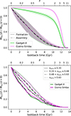 |
Fig. 1. Top: ICL formation (solid lines) and assembly (dash-dotted lines) histories of the 324 clusters for the two different simulation runs, GADGET-X (green) and GIZMO-SIMBA (magenta). The lines show the median values, with the masses normalised to the total ICL mass at z = 0, while the shaded regions correspond to the 16th to 84th percentile ranges. Bottom: ICL assembly history separating the clusters into four bins according to their formation time. The bins are selected to have approximately the same number of clusters in each bin. |
In this figure, we can see that the formation histories are significantly different for the two simulations, with GADGET-X showing continuous star formation, even at later times. While for GIZMO-SIMBA ∼99% of the stars are already formed by z ∼ 1, in GADGET-X there are only ∼80% of the stars formed by this redshift. This is consistent with Fig. 3 of Cui et al. (2022) that shows a much higher stellar fraction in the GIZMO-SIMBA clusters at z > 1, due to the more efficient star formation model followed by a rapid quenching due to intense AGN feedback. For a more detailed discussion, we refer to Section 4 in Cui et al. (2022).
Regarding the assembly histories, we see that both simulations agree almost perfectly. The assembly of the ICL happens, by definition, much later than the formation of its stars. According to Fig. 1, half of the present-day ICL mass was in place between z ∼ 0.2 and 0.5, while the other half was assembled after that. Going to higher redshifts, for instance z = 1, we can see that 10 to 30% of the final ICL was already in place by this redshift. We emphasise that these trends represent the assembly history of the z = 0 population, rather than the actual ICL content at earlier epochs, and are therefore not directly comparable to high-redshift observations. The similarity in the assembly histories is consistent with the fact that both simulations share the same initial conditions and dark matter halo assembly. This highlights that the ICL assembly is largely governed by the hierarchical growth of structure, whereas the differences in formation histories reflect the distinct baryonic physics models used in each simulation.
Given the size of our sample, we can also study how the assembly of the ICL varies from one cluster to another. In the top panel of Fig. 1 we can see that the shaded regions for the assembly histories, which correspond to the 16th–84th percentiles, are wider than for the formation histories. This means that, while (future) ICL stars are formed at similar times for all clusters, the time when they are assembled into the ICL changes more significantly from one cluster to another.
The bottom panel of Fig. 1 shows the assembly of the ICL, similar to the dash-dotted line in the top panel, but now separating the clusters into four bins according to their cluster formation time, zform. Following previous works with THE THREE HUNDRED simulations (e.g. Mostoghiu et al. 2019), zform is defined as the redshift at which M200 is equal to half its value at z = 0. The bins in the bottom panel of Fig. 1 are selected to ensure approximately the same number of clusters in each bin, for both GADGET-X and GIZMO-SIMBA. We find a clear trend, such that clusters that formed later (lower values of zform, solid lines), also assemble their ICL later. This points to a tight connection between the formation of the cluster and the build-up of its ICL. Previous works have shown that more dynamically evolved systems – i.e. those that are earlier assembled, more concentrated, or more relaxed – tend to host a higher fraction of their stellar mass in the ICL, both in simulations (Rudick et al. 2011; Cui et al. 2014; Contini et al. 2023; Contreras-Santos et al. 2024; Montenegro-Taborda et al. 2025) and observations (Montes & Trujillo 2018; Poliakov et al. 2021; Ragusa et al. 2023). Our results reinforce this picture from a theoretical perspective, showing that dynamically older clusters not only have more ICL, but also assemble it earlier.
3.2. Where: In situ vs ex situ
3.2.1. In situ fraction
Now that we know the timescales of ICL formation, the next step is to investigate where these stars formed. We are especially interested in the prevalence of in situ stars, formed directly within the ICL, which means that they already belong to the ICL at the moment of their formation. To identify these, we compare the assembly and formation times of all star particles that end up constituting the ICL at z = 0. In situ stars are those whose assembly time is equal to the formation time, that is, they were formed directly in the main cluster halo but not in any individual galaxy. We compute the total mass of in situ stars for each cluster and express it as a fraction of the total ICL massat z = 0.
Fig. 2 shows the distribution of this fraction across the 324 clusters, with solid green lines for GADGET-X and dash-dotted magenta for GIZMO-SIMBA. Vertical dotted lines indicate the median of each distribution. The figure reveals clear differences between the two simulations sets: GADGET-X produces a broad distribution, with some clusters reaching 20% of in situ ICL mass and a median value of 12.6%, while GIZMO-SIMBA yields a narrower distribution with a median value of 1.5%. These contrasting results suggest that there are different mechanisms at work in the simulations.
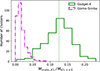 |
Fig. 2. Distribution of the fraction of in situ ICL mass for the 324 clusters in the GADGET-X (solid green line) and GIZMO-SIMBA (dash-dotted magenta line) runs. |
3.2.2. Distance to host centre
Given the significant in situ ICL fractions for GADGET-X clusters, we now explore more closely the formation of these stars. First, our definition for in situ requires that, when the star is formed, it belongs only to the main cluster halo, and not to any subhalo. We are not imposing any criteria in the distance from the centre at which the star is formed, so it could be the case that the star is formed very close to the centre, i.e. in the BCG, and then moved outwards so that at z = 0 it belongs to the ICL (see e.g. Section 3.3 in Ragone-Figueroa et al. 2018). To check for this situation, for the stars classified as in situ, we compute their distance to the main cluster centre at the time they were formed. In the left panel of Fig. 3 we show this distance, normalised by the radius R200 of the main cluster at the formation time of the star. We compute the distribution of the distances, weighted by particle mass, for each of the clusters, and then in Fig. 3 we show the median values for the set of the 324 clusters (solid lines), as well as the 16th to 84th percentiles as shaded regions. For GIZMO-SIMBA (depicted in magenta), we see that the distribution shows a prominent peak at r ∼ 0, indicating that the in situ star formation can be in fact associated with the central galaxy in the cluster. In contrast, GADGET-X (depicted in green) also shows a substantial population of stars at r ≲ 0.1 ⋅ R200, but with an extended distribution reaching up to ∼0.5 ⋅ R200. This suggests that a notable fraction of stars formed far from the cluster centre but not bound to any substructure at that time or later.
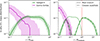 |
Fig. 3. Left: Distribution of distance from the in situ ICL particles to the main branch progenitor centre at the formation time of the particle, in units of the main branch halo radius R200. Green is for GADGET-X, magenta for GIZMO-SIMBA. Right: Distance from the in situ particles to the centre of the closest halo (or subhalo), in units of the radius of that halo, Rsubhalo. To ease comparison, we still show the distance to the main branch with the corresponding solid lines. The lines show the median computed stacking the 324 clusters; the shaded regions are the 16th–84th percentiles. |
For further investigation into this scenario, we now consider the distance to the closest subhalo at the formation time of the in situ star particle. In this way, we explore the possibility that these in situ particles not associated with the central galaxy are still associated with another galaxy, even if they are not identified as bound to it by the halo finder. To obtain this quantity, we compute the distance (in kpc) from each particle to all subhalos inside the cluster in the snapshot it was formed. We select the minimum distance in kpc and the subhalo associated to it and then we normalise by the radius of this subhalo. We note that the main cluster halo is included in this calculation, so it can also be selected as the closest substructure, although we do not specify this in the figure notation for simplicity. In the right panel of Fig. 3, similarly to the left one, we show the distribution of this distance, in units of Rsubhalo. As before, the situation for GIZMO-SIMBA is what could be expected, the particles are always formed in the centre of the halo they are associated to. However, the scenario is different for GADGET-X, for which, while there is also a peak at r ≲ 0.1 ⋅ R200, there is another peak at r ∼ Rsubhalo. This peak shows tails in both directions of the x-axis. To the right, this means that particles are being formed in the outer edges of subhalos and not bound to them. The tail to the left is more surprising, since it represents star particles formed inside subhalos without being bound to them.
3.2.3. Interpretation and discussion
Summarising the previous results, we find two different situations for our two simulations. For GADGET-X we have seen that the fraction of in situ ICL mass ranges from ∼5 to almost 20%. While most of the in situ stars are associated with the central galaxy, that is, formed in the centre of the cluster and then moved outwards, there is a significant fraction (∼35%) of in situ stars that are formed at a distance of more than ∼0.2 ⋅ R200 from the cluster centre. For GIZMO-SIMBA, the fraction of in situ ICL mass peaks at ∼1.5%, and for some clusters it reaches values of 5%. However, all the in situ star formation is associated with the central galaxy in this case.
To better understand the origin of non-central in situ stars in GADGET-X, we further examined the subhalo closest to each star at its formation time. While our approach is deliberately approximate and we do not include additional figures, it reveals clear and consistent trends. The reported numbers should be seen as lower limits, since associating objects based on physical distance may occasionally misidentify unrelated structures.
Analysing the gas content of the subhalos associated with in situ stars formed at r > 0.2 R200, we find that the great majority (∼80%) are strongly gas-dominated, with more than 90% of their total mass in gas. When identifying the closest companion to these gas-dominated subhalos, we find that in 70% of the cases it is a gas-free object, and in the remaining 30% it is another nearly pure gas blob. Given the nature of the merger trees, we cannot trace back in time such gas-dominated objects, but only those containing dark matter. Therefore, for the 70% of companions that do contain dark matter (that is, the gas-free ones), we compute their infall time and compare it with the formation time of the associated in situ ICL particles. We find that, at the time of ICL star formation, 60% of these companions have been inside the cluster for less than 2 Gyr, while also 60% of them have a velocity relative to the cluster that exceeds the cluster’s velocity dispersion, thus linking non-central in situ ICL to fast-moving, recently infalling subhalos.
These findings establish a clear scenario, in which a galaxy – initially composed of dark matter, stars and gas – falls into the cluster and experiences gas stripping. This process results in two distinct objects identified by the halo finder: a gas-dominated subhalo and a companion gas-free subhalo consisting of the leftover stars and dark matter. As the gas blob is decelerated at the cluster entrance, new stars can still form within it. However, since stars are collisionless, they quickly become unbound from the gas blob. In the first snapshot they appear, some of these stars can be already outside the gas blob, while others can remain inside but unbound, explaining the tails in both directions of r = Rsubhalo in the right panel of Fig. 3.
While this mechanism accounts for the in situ star formation outside the centre of the cluster, the question remains as to why these gas blobs form and whether they should survive or be shredded. A deep exploration of this topic would require a much more detailed study, which is out of the scope of this paper. However, we suggest that the gas may be stripped via ram-pressure stripping or artificially disrupted due to the different density regions the objects are going through (see e.g. Mostoghiu et al. 2021). The survival of the stripped blobs depends on how well the code deals with Kelvin-Helmholtz (KH) instabilities. SPH codes such as GADGET-X have been shown to struggle in dealing with these instabilities (Agertz et al. 2007), and so this scenario is favoured in GADGET-X. Additionally, the formation of the gas blobs also depends on the gas reservoir the galaxies retain, which is tied to the strength of galaxy feedback. In GIZMO-SIMBA, the stronger feedback implemented prevents the infalling galaxies from retaining enough gas for this scenario to occur. Together, these two aspects of the simulations – dealing with KH instabilities and galaxy feedback –, indicate that the fraction of non-central in situ star formation is highly simulation and code dependent and so very uncertain.
Comparing to similar works tracing the ICL particles in hydrodynamical simulations, some differences and similarities can be found. Using the TNG300 cosmological simulation of the IllustrisTNG project, Montenegro-Taborda et al. (2023) find a mean in situ ICL fraction of 11.4% for galaxy clusters, close to our GADGET-X fraction. In the TNG50 simulation within the same project, Ahvazi et al. (2024b) focus on three objects with masses ∼1014 M⊙ and find an in situ fraction that goes from 8 to 28%. Computing the distance to the cluster centre, they also find star formation out of the central region (out to 0.8 R200) that is not associated to any substructure, similarly to our GADGET-X results. However, Ahvazi et al. (2024b) further state that this star formation is not associated with ram pressure stripping of gas in infalling galaxies, but rather to small cloud-like objects condensing along filamentary structures that follow the neutral gas and dark matter distribution. Working with the EAGLE simulations, Proctor et al. (2024) find that, at the cluster scale, around 10% of the ICL mass is created in situ. In contrast, in a sample of 11 clusters from the HORIZON-AGN simulations, Brown et al. (2024) find that the contribution from in situ star formation to the ICL is negligible, more aligned with our results for GIZMO-SIMBA. The same is concluded by Joo et al. (2025) using a sample of more than 1200 groups and clusters from the Horizon Run 5 simulation.
These trends appear broadly consistent with the implications of our proposed mechanism. Simulations based on adaptive mesh refinement (AMR, e.g. RAMSES), such as HORIZON-AGN and Horizon Run 5, are better at capturing fluid instabilities and tend to suppress this kind of star formation, while SPH-based simulations such as EAGLE present substantial in situ ICL formation. The case of IllustrisTNG is more ambiguous: although it employs the moving mesh code AREPO, which is expected to better resolve instabilities, it still shows significant in situ ICL. This may be related to specific aspects of its feedback and star formation models, that allow stripped gas to cool and form stars under certain conditions. Overall, while our proposed scenario offers a possible explanation for these differences, a more definitive assessment would require targeted comparisons and deeper analysis.
3.3. How: Formation channels
In the previous subsection we have classified the ICL stellar particles into ex situ and in situ, depending on whether they were formed in a subhalo or directly in the host halo. Following these results (see Fig. 2), we now summarise this classification in Fig. 4. In the right panel of this figure we show, for GADGET-X on top and GIZMO-SIMBA on the bottom, the ICL mean mass composition of THE THREE HUNDRED clusters. The mean in situ mass fraction is, respectively, 12.5 and 1.7%. For the remaining star particles, the ex situ particles, we only know that they were formed in a different halo to the main one and at some point they started to be ICL particles. To further classify these particles, we focus on the snapshot prior to their assembly into the ICL and identify the halo they belonged to, that is, the halo that contributes them to the ICL. Taking into account the formation and assembly times of each ex situ star, and comparing with the position of its contributing halo relative to the main cluster halo at these times, we distinguish three different categories. In the three cases, the star has to be stripped from the contributing halo and moved into the main cluster halo, and so we call these three categories ‘stripped’, but including a prefix that denotes the different scenarios. These three categories are the following (see Fig. 4, left panel, for a schematic representation of the described processes):
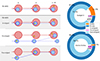 |
Fig. 4. Classification of the ICL star particles according to the way they were assembled into the ICL. Stellar particles are first classified into in situ and ex situ following Fig. 2, and then ex situ particles are classified into three different categories. On the left: Schematic representation of the different channels, with the main branch depicted in red and a secondary branch in blue. On the right: Mean value of the contribution from each channel for the 324 clusters in THE THREE HUNDRED sample. The top panel is for GADGET-X, the bottom panel for GIZMO-SIMBA. |
-
In-stripped stars: The particle is formed in a subhalo that is already inside the cluster and is later stripped into the ICL.
-
Pre-stripped stars: The particle is formed in a halo outside the cluster. It is stripped and enters the ICL before its own contributing halo falls into the cluster. We do not distinguish whether these halo afterwards falls inside the cluster or remains outside. The former can happen if the infalling halo grazes the cluster’s outskirts before eventually falling in. The latter can be either because the halo did not have enough time (i.e. the infall will be later than z = 0) or due to a fly-by, in which the star is torn by the cluster from the outer part of the halo. Since these stars represent a very low percentage we do not believe it necessary to check this scenario in more detail.
-
Post-stripped stars: The particle is formed in a halo outside the cluster, but it is now accreted into the ICL after its contributing halo falls into the cluster. The great majority of ex situ stars fall within this category.
In the right panel of Fig. 4 we can see that the ICL is widely dominated by the post-stripped stars, stripped from a halo after its infall into the host cluster. If we consider only the ex situ mass, post-stripped stars represent around 90% for both simulations. For this reason, we devote the next section to a deeper study of this component of the ICL.
The second most important contribution comes from stars that are also stripped but that were formed in a halo after its infall into the host cluster. They are more frequent in GADGET-X, which is reasonable given that this simulation has a more significant late star formation (see Fig. 1). We also note that, in the GADGET-X run, around 30% of these in-stripped stars are formed within a subhalo that is gas-dominated, similarly to the non-central in situ star formation discussed in Section 3.2.3. In this case, the star is still bound to the gas blob when formed, and so it is not considered in situ. As before, this scenario does not occur in GIZMO-SIMBA, where in-stripped stars represent a lower fraction of the total ICL, and are all associated to objects that are not gas-dominated.
We note that our distinction between pre- and post-stripped stars only depends on whether the star is contributed to the ICL by a halo before or after its infall into the host halo. The contributing halo can be a small subhalo or a large halo merging with the central one. We thus do not check if the particle was previously in a galaxy or already ICL of a merging cluster. For instance, if a particle belongs to the diffuse component (intragroup light, IGL) of an infalling group, and the group crosses R200 of the host halo before the particle is accreted into the host cluster’s ICL, this star would be classified as post-stripped. Determining whether stars were already ICL in their original halos requires further study, which we leave for future work. Similarly, we do not consider here the fate of the contributing halos after their particles are stripped. A more detailed analysis is required to determine whether they merge with the BCG, survive as subhalos in the cluster or are totally disrupted, that we also leave for a follow-up work.
4. Post-stripped ICL
As discussed in the previous section, the majority of the ex situ ICL stars are classified as post-stripped, that is, stars that were stripped from infalling halos after they crossed into the host cluster’s R200. In this section, we focus on this dominant component by analysing the halos that contribute these stars and their role in building up the ICL.
4.1. Properties of contributing halos
We have previously obtained the information about which halos bring the star particles into the ICL. We now examine the properties of these halos. To enable consistent comparisons between different halos, we consider their properties at their infall time, defined as the last snapshot in which the halo is outside R200 of the host cluster. For halos that have more than one infall, we only consider the first one. This way, we ensure that the halos are mostly unaltered by their infall into the cluster, and so their properties remain unbiased.
Throughout this section, we only work with the post-stripped stars (see Section 3.3) and use the term ICLpost to refer to this component. We exclude the in-stripped and pre-stripped categories to ensure consistency and to highlight distinct pathways of ICL formation. In-stripped stars form from the remaining gas of a subhalo already inside the cluster, while pre-stripped stars originate from a halo that may never enter the cluster, making their infall time ill-defined. By concentrating on the dominant post-stripped population, we ensure a clear and consistent analysis of this accretion process.
In Fig. 5 we show the distribution of the relative contribution to the post-stripped ICL from the different halos. We consider the ICLpost at z = 0 of each of the 324 clusters and, for each star particle, we get the mass at (first) infall of its contributing halo, both stellar and total (including also dark matter and gas). The left column of Fig. 5 focuses on the stellar mass distribution. For each cluster, we compute the cumulative contribution of infalling stellar masses, and then derive the median across all clusters (solid green lines for GADGET-X, dash-dotted magenta for GIZMO-SIMBA), with shaded regions indicating the 16th–84th percentiles. Horizontal dotted lines mark the 25, 50, and 75% cumulative contribution levels.
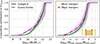 |
Fig. 5. Cumulative distribution of the mass contribution to the post-stripped ICL from halos of different infall masses. The left column is for stellar mass at infall; the right column is for the total mass ratio to the host at infall time. The lines depict the distributions obtained as the median of the individual distributions for each cluster, while the shaded regions indicate the 16th–84th percentiles. The green solid lines are for GADGET-X and the magenta dash-dotted lines for GIZMO-SIMBA. In the right column, the yellow and brown shaded regions indicate the minor (1:10 to 1:3) and major merger regimes (1:3 to 1:1). The horizontal dotted lines indicate fractions of 0.25, 0.5, and 0.75 of the post-stripped ICL. |
At the low-mass end, both simulations show a tail of contributing halos that extends down to the resolution limit – mean stellar particle mass is ∼0.6 ( ∼ 2)⋅108 M⊙ for GADGET-X (GIZMO-SIMBA). While the contribution from these low-mass halos is small, GIZMO-SIMBA predicts a slightly higher relative importance compared to GADGET-X. Despite some incompleteness due to resolution, this is unlikely to strongly affect our results. Higher-resolution hydrodynamical simulations (e.g. Brown et al. 2024, with stellar mass resolution of ∼2 ⋅ 106 M⊙; or Ahvazi et al. 2024a) have shown that halos with stellar mass ≲109 M⊙ contribute less than 10% of the ICL mass. Moving to higher masses, the left panel of Fig. 5 shows that half of the post-stripped ICL is contributed by halos with a stellar mass above 1011.4 − 12.1 M⊙, with the distribution extending up to ∼1012.5 M⊙. Both simulations show excellent agreement in this regime. These high stellar masses correspond to the stellar component of massive groups and clusters, indicating that there are major mergers involved in the formation of the ICL.
We study this in the right panel of Fig. 5, in which we follow the same procedure to plot the cumulative distribution of the total mass ratio between the host and the contributing halo at its infall time. As before, the distribution is skewed left, with a tail that reaches values of the mass ratio smaller than 10−4. The shaded yellow and brown regions indicate the typical mass ratio ranges associated with minor (1:10 to 1:3) and major (1:3 to 1:1) mergers (e.g. Planelles & Quilis 2009; Contreras-Santos et al. 2022). Infalling objects with a mass ratio below 1:10 are generally considered as very minor mergers or smooth accretion. These low-mass contributors account for roughly 20−50% of the ICLpost mass in GADGET-X, and 30−55% in GIZMO-SIMBA, which again shows a slightly larger contribution from lower-mass halos. The remaining mass is brought in through minor and major mergers, which contribute medians of around 25 and 35%, respectively, though with considerable scatter among clusters, as shown by the shaded regions. The plot also shows a small contribution from mergers with a ratio > 1, which indicates that the merging object is larger than the one considered the host. This is due to the way the merger trees are built, which is such that the main progenitor does not always have to be the most massive progenitor (see Section 2.3). In this way, it can be the case that a bigger halo merges with the main branch halo, bringing some of its mass into the host’s ICL. Although not very often, this situation happens sometimes, and contributes some mass to the formation of the ICL of massive clusters.
In general, Fig. 5 shows how massive galaxies, groups and even other clusters are responsible for building up the ICL of galaxy clusters as massive as those in THE THREE HUNDRED sample. It is important to note that, according to Martin et al. (2024), the dark matter resolution plays a critical role in accurately capturing the stripping process of galaxies, more so than the stellar resolution. Poorly resolved halos can have their stellar material over-stripped, potentially affecting even relatively massive halos. While this issue is particularly relevant for low-mass objects, which may contribute slightly more than our results suggest, it has less impact on very massive objects, which are well resolved in our simulations. Thus, we emphasise the significant contribution from these massive systems in building the ICL.
To complete this picture of infalling halos that bring the ICL particles into the cluster, Fig. 6 shows the distribution of the infall redshift of the contributing halos, computed as the redshift of the last snapshot in which the halo is outside R200 of the host cluster. We can see that the maximum values are around z ∼ 4, while the contributions start to become more significant at redshift around 2. This is consistent with the assembly history in Fig. 1, which indicates the time when the stars were accreted into the ICL and shows no ICL growth at z ∼ 4. By definition, post-stripped stars have to enter the cluster before becoming ICL, and so the infall redshifts in Fig. 6 have to be higher than those at which the ICL starts growing in Fig. 1. In addition, Fig. 6 shows that most halos infall at z ∼ 1. We also remind here that, for halos that have more than one infall, we only consider the first one.
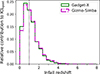 |
Fig. 6. Distribution of the relative mass contribution to the post-stripped ICL from halos with different infall times. The values for the 324 clusters have been stacked together to produce the distributions for GADGET-X (green) and GIZMO-SIMBA (magenta). The vertical dotted lines indicate the median values of each distribution. |
4.2. Number of accreted halos
We have already selected all the halos that contribute to construct the post-stripped ICL of the simulated clusters, and we have studied the mass, mass ratio, and infall time of these objects. Now, we can focus on the contribution that each halo makes to the ICLpost of the cluster. For each of the contributing halos, we sum up the mass of all the particles that it contributes at any time, and we normalise this mass by the ICLpost mass at z = 0 of the cluster. Then, we order the contributing halos by this value (halos that contribute the most go first) and create a cumulative distribution, showing the summed ICLpost fraction as a number of the involved halos. We repeat this procedure for each of the 324 clusters, and in Fig. 7 we show the median distribution together with 16th to 84th percentiles (shaded regions). Essentially, this figure is showing the minimum number of accreted halos needed for a median cluster to assemble a given fraction of its ICLpost. We can see in Fig. 7 that already the most contributing halo can reach up to 40% of the final ICLpost mass. To reach 50% of their ICLpost mass (indicated with a horizontal line), clusters need a minimum of 2−8 accreted objects for both simulations. The situation starts to differ for them at higher values. For instance, 80% of the ICLpost is built with 8 to 22 halos for GADGET-X, while GIZMO-SIMBA requires a minimum number between 15 and 70. For the whole post-stripped ICL at z = 04, the differences become even larger, with 75 to 150 halos needed for GADGET-X and 300 to 600 for GIZMO-SIMBA. This is in agreement with the results from Fig. 5, which showed that the contributing halos are less massive in GIZMO-SIMBA. A possible explanation is that galaxies in GIZMO-SIMBA develop denser stellar cores than those in GADGET-X (Meneghetti et al. 2023), making them less susceptible to tidal stripping. As a result, larger galaxies in GIZMO-SIMBA are more likely to retain their identity rather than contributing to the ICL, while smaller satellites, which are more easily disrupted, dominate the ICL build-up. On the other hand, in GADGET-X, lower-mass galaxies are more susceptible to disruption, sometimes even before reaching R200, which prevents them from contributing to the ICL. This could explain why GIZMO-SIMBA has a higher contribution from low-mass halos (see e.g. Dolag et al. 2009, for a detailed study on the survival rates of infalling substructures in hydrodynamical simulations).
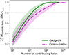 |
Fig. 7. Median number of accreted halos required to assemble the ICLpost. The lines indicate the median distribution (solid green for GADGET-X, dash-dotted magenta for GIZMO-SIMBA), while the shaded regions denote the 16th–84th percentiles. The halos are ordered starting from the one that contributes the most, and the values on the y-axis are the cumulative contribution of all previous halos, normalised by the ICLpost mass at z = 0. The horizontal lines indicate fractions of 0.5 and 0.8 on the y-axis, for reference. |
For further investigation into the halos that build the ICL of clusters, we present in Fig. 8 different density plots with the scatter between some of their properties. Top row is for GADGET-X, bottom one for GIZMO-SIMBA. In this figure, we are showing 2D histograms coloured by the number of accreted halos within each region of the plot, stacking the 324 clusters together. The scale in the colourbar is the same for the two simulations, highlighting that, as we already saw in Fig. 7, the number of accreted halos is higher for GIZMO-SIMBA. The first column shows the infall redshift of the contributing halos against the mass ratio to the host cluster mass at this time. We can see that there is a positive correlation, such that halos that infall earlier have a mass ratio to the host that is closer to 1. This is quantified by the Spearman correlation coefficient, displayed in the top-left corner of each panel, which confirms the strength and significance of the correlation. This result aligns with expectations from the ΛCDM hierarchical formation scenario, in which major mergers are more frequent at higher redshifts (see e.g. Fig. 2 in Nuza et al. 2024 for the galaxy cluster major merger rate as a function of redshift in THE THREE HUNDRED simulations). In the second column of Fig. 8, we plot on the y-axis the mass contribution to the cluster’s ICL of each halo, computed as in Fig. 7, Mcontrib, halo/MICLpost, as a function of the infall redshift. The trend is weaker now, as quantified by the Spearman correlation coefficient in the bottom corner, but we again see a positive correlation such that earlier infallers, which are less frequent, contribute a higher fraction to the ICL of the cluster. In the third column, the y-axis still shows the contribution from each halo but as a function of the mass ratio to the host cluster. Consistently with expectations and with the previous scenario, halos with a ratio closer to 1 are those that contribute the most to the ICL of the cluster, although the most common events are those that bring around 10−3 to 10−4 of the ICL mass and have a mass ratio of similar value. While the correlation between the mass contributed and the mass ratio is strong (rs ∼ 0.6), the figure shows a large scatter. This scatter likely reflects the importance of additional factors such as the orbits of the accreted halos. For instance, halos on more elliptical orbits experience stronger tidal disturbances during close passages, potentially leading to larger contributions to the ICL. We leave a detailed study of halo orbits and stripping processes for a follow-up paper.
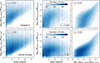 |
Fig. 8. Two-dimensional histograms showing the distribution of the events that build the ICLpost. The top row is for GADGET-X, the bottom row for GIZMO-SIMBA. The first column shows the scatter plot between infall redshift and mass ratio to the host cluster, coloured by the number of accreted halos. The second and third columns show the total mass that each halo contributed to the ICLpost of the involved cluster, as a function of infall redshift and mass ratio of the event. The Spearman correlation coefficients, rs, are shown in each panel. |
4.3. Contribution to post-stripped ICL
To sum up the conclusions from Fig. 8 and further establish the general scenario for the formation of the ICL in THE THREE HUNDRED clusters, in Fig. 9 we show a 2D histogram between the mass ratio of the infalling halo to the host and the infall redshift, with the density weighted by the contribution to the total post-stripped ICL of clusters. This means that, instead of plotting the number of accreted halos as in Fig. 8, we now weigh each event by the mass it contributes to its cluster’s ICL, Mcontrib, halo/MICLpost. We stack the accreted halos for all the clusters and thus divide the weights by the total number of clusters in the sample, 324, leading to the colourbar in the right of Fig. 9.
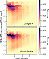 |
Fig. 9. Similar to Fig. 8, 2D histogram showing the distribution of the accreted halos that build the ICLpost (top for GADGET-X; bottom for GIZMO-SIMBA). Here the colouring is weighted by the fraction of mass that each halo contributes to the total ICLpost summed across all clusters. The x-axis shows the mass ratio of the halo to the host at infall, and the y-axis shows the corresponding infall redshift. |
For both simulations (GADGET-X on top, GIZMO-SIMBA on the bottom), Fig. 9 shows that the dominant contribution to the ICLpost comes from halos that infall at redshift around 1 or below, with mass ratios between 1:10 and 1:1. While Fig. 8 showed that, individually, early infallers contribute more mass per halo, the more frequent later infallers accumulate to a greater total contribution. Halos accreted earlier, until redshift around ≲2, with mass ratios above 1:10, also contribute significantly to the ICL of clusters. The remaining ICLpost mass arises from numerous minor events, halos with mass ratios below 1:10 and down to 10−3 or 10−4, typically infalling between z ∼ 3 and z ∼ 1. As in Fig. 5, we see a small contribution from mergers with a ratio > 1. In the third column of Fig. 8 we have seen that these events are not very common (see density of halos), but they bring a very significant fraction of the ICL, and so in the end they can be fairly relevant for the assembly of the ICL of massive clusters.
4.4. Discussion
In this section we have focused on the post-stripped component of the ICL, made of stars that were brought into the cluster within a halo and, after that, became unbound from it and bound to the cluster’s potential. We have seen that these contributing halos are generally massive halos. In fact, 65 to 80% of the ICL mass is brought in by infalling objects with stellar mass M* > 1011 M⊙. Looking instead at the total mass of the infalling objects and computing the mass ratio to the cluster’s mass, we show that a median of around 35% of the ICL comes from major mergers. As for the redshift distribution, the infall time of these objects peaks at z ∼ 1, with a tail that reaches until z ∼ 4. Considering each contributing halo an ‘event’ that takes part in the assembly of the ICL, we have computed the ICL fraction contributed by each event. We have seen that, while the most common events are those happening recently and with a very low mass ratio, the ones that contribute the most generally present a high mass ratio and happen at higher redshifts. Adding up all the relative contributions, we conclude that the most relevant contributions to the ICL come from halos with a mass ratio between 1:10 and 1:1, infalling at redshift ≲1.
Comparing to previous theoretical works, our results appear consistent with the general trends, while also extending the analysis to a larger sample of more massive clusters. Based on semi-analytic models of galaxy formation and N-body simulations, Contini et al. (2014) found that around 68% of the ICL mass comes from satellites more massive than 1010.5 M⊙. This is in agreement with the prior analytical model by Purcell et al. (2007), which shows that the ICL is dominated by material liberated from galaxies with M* ∼ 1011 M⊙. Martel et al. (2012) find slightly smaller galaxies, with 109 M⊙ < M* < 1010.5 M⊙ to be the major contributors to the ICL (∼60%). All these works agree that the contribution from dwarf galaxies is negligible, even if they dominate in terms of numbers, similarly to our results in Fig. 8, where we show that the most common and less contributing events are those with lower mass ratios. Further work with semi-analytic models by Contini et al. (2019), comparing typical colours of the ICL with those of satellites with different masses, concludes that, at earlier times (z ∼ 1), the most important contributors to ICL are galaxies with 9 < log M*/M⊙ < 10, while at lower redshifts (z ∼ 0.5 and below), more massive galaxies (up to 1011 M⊙) contribute most. This is in agreement with our Fig. 9, which shows that objects with a higher mass ratio to the host contribute more at later times.
Working with hydrodynamical simulations of galaxy clusters, Brown et al. (2024) find that dominant contributors to ICL are galaxies with stellar mass between 1010.5 and 1011 M⊙ at their infall time. Ahvazi et al. (2024a), also with hydrodynamical simulations but with less massive clusters and massive groups, find 50% of the ICL to come from galaxies more massive than 1010 M⊙. These works also agree that the dispersion between clusters is wide, which is related to the ICL being formed from very massive objects, so that for an individual cluster the situation can vary greatly. Similarly, Cooper et al. (2015) show that the ICL is very sensitive to contributions of progenitors with a mass ratio of 1:10 (see also Harris et al. 2017), matching our Fig. 9 results, that highlight the contribution from major mergers to the ICL. In contrast to this, analysing mock images from hydrodynamical simulations, Tang et al. (2023) find that the contribution from most massive galaxies to the ICL is minimal, and the dominant ones are within 8 < log M*/M⊙ < 10. With a different set of simulations, Chun et al. (2023) find that half of the ICL and BCG components comes from objects with M∗ > 1011 h−1 M⊙ in unrelaxed clusters (and from slightly less massive objects for relaxed clusters). In a follow up work, Chun et al. (2024) confirm that typical ICL progenitors fall into the clusters with intermediate mass (10 < log M*/M⊙ < 11), with high-mass infallers being more important for dynamically unrelaxed and more massive clusters.
Our results regarding the mass of the contributing objects, as shown in Fig. 5, are overall in agreement with previous works (except for Tang et al. 2023). Although our objects are in general more massive (we find a median of 1011.7 M⊙), it is important to note that our host clusters, with M200 > 6.3 ⋅ 1014 M⊙, are also the most massive across all the mentioned studies, and so it is expected that they are formed by more massive contributors (e.g. Chun et al. 2024).
5. Conclusions
With the advent of new and modern telescopes such as Rubin, Euclid, and JWST, the field of the low surface brightness universe, and specifically of the ICL, has attracted the interest of the scientific community. New studies show very promising avenues to extract all the information encoded in the ICL, for instance the first ICL study of a cluster with JWST data (Montes & Trujillo 2022), the study of the ICL of the Perseus cluster using Euclid Early Release Observations (Kluge et al. 2025), and the first spectro-photometric analysis of the entire ICL in a cluster with joint JWST, HST, and MUSE data (Jiménez-Teja et al. 2024). In this context, it becomes essential to have theoretical models that can explain the observations and describe the different astrophysical processes involved. In our previous work (Contreras-Santos et al. 2024), we introduced the ICL of THE THREE HUNDRED clusters. We showed that it is overall consistent with observations and presented some of its properties at the present day. In this paper, we provided a theoretical scenario for the formation of the ICL in very massive clusters. In order to do this, we started with the ICL at z = 0 and traced its particles back in time. Following these particles through the different snapshots of the simulations, we studied when, where, and how they assemble into the ICL component of the simulated clusters.
THE THREE HUNDRED project consists of a suite of 324 spherical regions centred on the most massive clusters found in a prior dark matter-only cosmological simulation. These regions, of 15 h−1 Mpc in radius, have been resimulated including full hydrodynamics in two different implementations: GADGET-X, which uses a modified version of the non-public GADGET3 code (Murante et al. 2007; Rasia et al. 2015); and GIZMO-SIMBA, performed with the GIZMO code (Hopkins 2015) and the galaxy formation subgrid models from the SIMBA simulation (Davé et al. 2019). The initial conditions are the same for both resimulations, and so we can consistently compare the resulting clusters, which is interesting to test the robustness of the predictions and understand the effects of the different modelling. Our sample constitutes a mass-complete sample within the range 14.8 < log(M200/M⊙) < 15.6 at z = 0. With 324 clusters within this mass, it is a large set of galaxy clusters, similar in statistics to the TNG-Cluster (Nelson et al. 2024), MillenniumTNG (Pakmor et al. 2023) or FLAMINGO (Schaye et al. 2023) simulations, but much larger than other cluster simulations such as Cluster-EAGLE (Barnes et al. 2017) or DIANOGA (Bassini et al. 2020), with one order of magnitude fewer clusters.
The main findings of this work can be summarised asfollows:
-
Half of the ICL present-day mass was already in the ICL at redshifts between z ∼ 0.2 and 0.5. At redshift z ∼ 1, between 10 and 30% of the final ICL was in place (see Fig. 1, top). The two codes show perfect agreement on this, although the stars that were to become ICL in GADGET-X were formed significantly later than those in the GIZMO-SIMBA run. In addition, both simulations show that clusters that formed earlier also assemble their ICL earlier (Fig. 1, bottom), highlighting the close connection between the ICL component and the whole cluster (including the dark matter halo).
-
We define in situ stars as those formed directly in a progenitor of the central halo and not in any other object. GADGET-X shows a fraction of in situ stars between 5 and 20% of the total ICL, while GIZMO-SIMBA shows a median value of 1.5%, with the highest values being around 5%.
-
Studying the distance from the in situ stars to the cluster centre at the time of their formation (Fig. 3), we find that the in situ stars in GIZMO-SIMBA can be associated to the BCG, being formed in the centre and ejected later into the ICL. In GADGET-X, around 35% of the in situ stars are formed at a distance r ≳ 0.2 R200 from the cluster centre. The origin of these particles in GADGET-X, and whether it is physical or numerical, remains unclear, since an in-depth investigation is beyond the scope of this paper, but we find them to be associated with gas-dominated blobs likely formed due to the disruption or ram-pressure stripping of recent infalling halos.
-
We classify the remaining ICL stellar particles (ex situ stars) based on the halo they belonged to before being accreted to the ICL and on when this happened. The major contribution is from post-stripped stars (∼90% of ex situ stars; see Fig. 4) that fell into the cluster inside another halo and later became unbound from it and bound to the cluster halo. Other minor contributions are from stars formed in a subhalo already inside the cluster and then stripped from it, stars accreted into the ICL from a halo that was still outside the cluster halo before its infall, and stars contributed by halos that never fall into the cluster.
-
Focusing only on the post-stripped ICL, we find that, depending on the cluster, 65 to 80% of the total ICL is brought in by objects with M* > 1011 M⊙ at their infall time. In terms of total mass ratio of these objects to the cluster, major mergers involve, in median, around 35% of the mass in the post-stripped ICL, ranging from around 15 to 55% for the different clusters.
-
Studying these events that make up the post-stripped ICL in more detail, we show in Fig. 8 that the most common events are recent infallers with a very low mass ratio (very minor mergers or slow accretion). However, the higher the infall redshift and the mass ratio of the halo to the host cluster, the higher is the fraction that this halo contributes to the ICL. Stacking all the clusters together, in Fig. 9 we see that the main channel to build ICL is from minor or major mergers at z ≤ 1, in agreement with the previous results. Halos with a mass ratio close to 1, but with higher infall redshift, between 1 and 2, also contribute a relevant fraction, while the remaining mass comes from very minor mergers or accretion at redshifts 1 ≲ z ≲ 3.
-
Finally, in Fig. 7 we present the minimum number of accreted halos needed to assemble any fraction of the post-stripped ICL. For both implementations of the hydrodynamics, a minimum of two to eight halos is needed to build 50% of the ICL. For the whole ICL the results differ notably, with GADGET-X requiring between 75 and 150 halos, and GIZMO-SIMBA 300 to 600. The mass of these halos also differs from one simulation to another; GIZMO-SIMBA shows a more important contribution from smaller subhalos that infall into the main cluster (Fig. 5).
In summary, we find that the build-up of the ICL is mainly due to very massive galaxies as well as major mergers with other massive groups or clusters, preferentially happening at redshifts below 1. We note that we do not distinguish between mergers and stripping throughout this work; in other words, we do not take into account whether the contributing halos end up being disrupted or they survive as subhalos of the host cluster. We also do not check whether the halos merge first with the BCG and the stars move to the ICL afterwards. These aspects will be the focus of a forthcoming follow-up study, where we will analyse in more detail the properties of contributing halos. In particular, we will investigate whether the contributing stars were already part of a diffuse component in their original halos, and we will characterise the stripping process itself by examining the orbital parameters, the cosmic web environment, the stripping timescales, the fraction of mass lost, and related dynamical properties.
See Springel (2005) for a detailed description of the last public version GADGET-2.
The total stellar content of a cluster refers to all bound particles within R200.
We compute this value using 99% of the ICLpost instead of 100, in order to avoid counting minimal contributions.
Acknowledgments
This work has been made possible by THE THREE HUNDRED (https://the300-project.org) collaboration. The simulations used in this paper have been performed in the MareNostrum Supercomputer at the Barcelona Supercomputing Center, thanks to CPU time granted by the Red Española de Supercomputación. As part of THE THREE HUNDRED project, this work has received financial support from the European Union’s Horizon 2020 Research and Innovation programme under the Marie Sklodowskaw-Curie grant agreement number 734374, the LACEGAL project. ACS, AK, GY, IAA and CDV thank the Ministerio de Ciencia e Innovación (MICINN) for financial support under research grants PID2021-122603NB-C21 and PID2021-122603NB-C22. AK further thanks My Bloody Valentine for loveless. WC is supported by the Atracción de Talento Contract no. 2020-T1/TIC19882 granted by the Comunidad de Madrid in Spain, and the science research grants from the China Manned Space Project. He also thanks the Ministerio de Ciencia e Innovación (Spain) for financial support under Project grant PID2021-122603NB-C21 and HORIZON EUROPE Marie Sklodowska-Curie Actions for supporting the LACEGAL-III project with grant number 101086388. SEN is a member of the Carrera del Investigador Científico of CONICET. He acknowledges support from CONICET (PIBAA R73734) and Agencia Nacional de Promoción Científica y Tecnológica (PICT 2021-GRF-TI-00290).
References
- Agertz, O., Moore, B., Stadel, J., et al. 2007, MNRAS, 380, 963 [NASA ADS] [CrossRef] [Google Scholar]
- Ahvazi, N., Sales, L. V., Doppel, J. E., et al. 2024a, MNRAS, 529, 4666 [NASA ADS] [CrossRef] [Google Scholar]
- Ahvazi, N., Sales, L. V., Navarro, J. F., et al. 2024b, Open J. Astrophys., 7, 111 [CrossRef] [Google Scholar]
- Alonso Asensio, I., Dalla Vecchia, C., Bahé, Y. M., Barnes, D. J., & Kay, S. T. 2020, MNRAS, 494, 1859 [CrossRef] [Google Scholar]
- Barfety, C., Valin, F.-A., Webb, T. M. A., et al. 2022, ApJ, 930, 25 [NASA ADS] [CrossRef] [Google Scholar]
- Barnes, D. J., Kay, S. T., Bahé, Y. M., et al. 2017, MNRAS, 471, 1088 [Google Scholar]
- Bassini, L., Rasia, E., Borgani, S., et al. 2020, A&A, 642, A37 [NASA ADS] [CrossRef] [EDP Sciences] [Google Scholar]
- Beck, A. M., Murante, G., Arth, A., et al. 2016, MNRAS, 455, 2110 [Google Scholar]
- Behroozi, P. S., Wechsler, R. H., & Wu, H.-Y. 2013, ApJ, 762, 109 [NASA ADS] [CrossRef] [Google Scholar]
- Biffi, V., Planelles, S., Borgani, S., et al. 2017, MNRAS, 468, 531 [Google Scholar]
- Bondi, H. 1952, MNRAS, 112, 195 [Google Scholar]
- Brough, S., Ahad, S. L., Bahé, Y. M., et al. 2024, MNRAS, 528, 771 [NASA ADS] [CrossRef] [Google Scholar]
- Brown, H. J., Martin, G., Pearce, F. R., et al. 2024, MNRAS, 534, 431 [NASA ADS] [CrossRef] [Google Scholar]
- Burke, C., Hilton, M., & Collins, C. 2015, MNRAS, 449, 2353 [Google Scholar]
- Cañas, R., Lagos, C. D. P., Elahi, P. J., et al. 2020, MNRAS, 494, 4314 [Google Scholar]
- Canepa, L., Brough, S., Lanusse, F., Montes, M., & Hatch, N. 2025, ApJ, 980, 245 [Google Scholar]
- Chen, X., Zu, Y., Shao, Z., & Shan, H. 2022, MNRAS, 514, 2692 [NASA ADS] [CrossRef] [Google Scholar]
- Chun, K., Shin, J., Smith, R., Ko, J., & Yoo, J. 2023, ApJ, 943, 148 [NASA ADS] [CrossRef] [Google Scholar]
- Chun, K., Shin, J., Ko, J., Smith, R., & Yoo, J. 2024, ApJ, 969, 142 [Google Scholar]
- Contini, E. 2021, Galaxies, 9, 60 [NASA ADS] [CrossRef] [Google Scholar]
- Contini, E., De Lucia, G., Villalobos, Á., & Borgani, S. 2014, MNRAS, 437, 3787 [Google Scholar]
- Contini, E., Yi, S. K., & Kang, X. 2019, ApJ, 871, 24 [Google Scholar]
- Contini, E., Chen, H. Z., & Gu, Q. 2022, ApJ, 928, 99 [NASA ADS] [CrossRef] [Google Scholar]
- Contini, E., Jeon, S., Rhee, J., Han, S., & Yi, S. K. 2023, ApJ, 958, 72 [NASA ADS] [CrossRef] [Google Scholar]
- Contini, E., Rhee, J., Han, S., Jeon, S., & Yi, S. K. 2024, AJ, 167, 7 [NASA ADS] [CrossRef] [Google Scholar]
- Contreras-Santos, A., Knebe, A., Pearce, F., et al. 2022, MNRAS, 511, 2897 [NASA ADS] [CrossRef] [Google Scholar]
- Contreras-Santos, A., Knebe, A., Cui, W., et al. 2024, A&A, 683, A59 [NASA ADS] [CrossRef] [EDP Sciences] [Google Scholar]
- Cooper, A. P., Gao, L., Guo, Q., et al. 2015, MNRAS, 451, 2703 [Google Scholar]
- Cui, W., Murante, G., Monaco, P., et al. 2014, MNRAS, 437, 816 [Google Scholar]
- Cui, W., Knebe, A., Yepes, G., et al. 2018, MNRAS, 480, 2898 [Google Scholar]
- Cui, W., Dave, R., Knebe, A., et al. 2022, MNRAS, 514, 977 [NASA ADS] [CrossRef] [Google Scholar]
- Davé, R., Thompson, R., & Hopkins, P. F. 2016, MNRAS, 462, 3265 [Google Scholar]
- Davé, R., Anglés-Alcázar, D., Narayanan, D., et al. 2019, MNRAS, 486, 2827 [Google Scholar]
- De Lucia, G., & Blaizot, J. 2007, MNRAS, 375, 2 [Google Scholar]
- DeMaio, T., Gonzalez, A. H., Zabludoff, A., Zaritsky, D., & Bradač, M. 2015, MNRAS, 448, 1162 [NASA ADS] [CrossRef] [Google Scholar]
- DeMaio, T., Gonzalez, A. H., Zabludoff, A., et al. 2018, MNRAS, 474, 3009 [Google Scholar]
- DeMaio, T., Gonzalez, A. H., Zabludoff, A., et al. 2020, MNRAS, 491, 3751 [Google Scholar]
- Dolag, K., Borgani, S., Murante, G., & Springel, V. 2009, MNRAS, 399, 497 [Google Scholar]
- Dolag, K., Murante, G., & Borgani, S. 2010, MNRAS, 405, 1544 [NASA ADS] [Google Scholar]
- Edwards, L. O. V., Salinas, M., Stanley, S., et al. 2019, MNRAS, 491, 2617 [Google Scholar]
- Feldmeier, J. J., Mihos, J. C., Morrison, H. L., et al. 2004, ApJ, 609, 617 [Google Scholar]
- Fu, H., Shankar, F., Ayromlou, M., et al. 2024, MNRAS, 532, 177 [NASA ADS] [CrossRef] [Google Scholar]
- Furnell, K. E., Collins, C. A., Kelvin, L. S., et al. 2021, MNRAS, 502, 2419 [NASA ADS] [CrossRef] [Google Scholar]
- Gill, S. P. D., Knebe, A., & Gibson, B. K. 2004, MNRAS, 351, 399 [Google Scholar]
- Golden-Marx, J. B., Zhang, Y., Ogando, R. L. C., et al. 2023, MNRAS, 521, 478 [Google Scholar]
- Gonzalez, A. H., Zabludoff, A. I., & Zaritsky, D. 2005, ApJ, 618, 195 [Google Scholar]
- Gonzalez, A. H., Sivanandam, S., Zabludoff, A. I., & Zaritsky, D. 2013, ApJ, 778, 14 [Google Scholar]
- Harris, K. A., Debattista, V. P., Governato, F., et al. 2017, MNRAS, 467, 4501 [NASA ADS] [CrossRef] [Google Scholar]
- Hlavacek-Larrondo, J., Rhea, C. L., Webb, T., et al. 2020, ApJ, 898, L50 [NASA ADS] [CrossRef] [Google Scholar]
- Hopkins, P. F. 2015, MNRAS, 450, 53 [Google Scholar]
- Hopkins, P. F. 2017, ArXiv e-prints [arXiv:1712.01294] [Google Scholar]
- Hopkins, P. F., & Quataert, E. 2011, MNRAS, 415, 1027 [NASA ADS] [CrossRef] [Google Scholar]
- Hopkins, P. F., Kereš, D., Oñorbe, J., et al. 2014, MNRAS, 445, 581 [NASA ADS] [CrossRef] [Google Scholar]
- Iodice, E., Spavone, M., Cantiello, M., et al. 2017, ApJ, 851, 75 [Google Scholar]
- Janowiecki, S., Mihos, J. C., Harding, P., et al. 2010, ApJ, 715, 972 [Google Scholar]
- Jiménez-Teja, Y., Gimenez-Alcazar, A., Dupke, R. A., et al. 2024, ApJ, 974, 309 [CrossRef] [Google Scholar]
- Joo, H., & Jee, M. J. 2023, Nature, 613, 37 [NASA ADS] [CrossRef] [Google Scholar]
- Joo, H., Jee, M. J., Kim, J., et al. 2025, ApJ, 990, 96 [Google Scholar]
- Kluge, M., Hatch, N. A., Montes, M., et al. 2025, A&A, 697, A13 [NASA ADS] [CrossRef] [EDP Sciences] [Google Scholar]
- Klypin, A., Yepes, G., Gottlöber, S., Prada, F., & Heß, S. 2016, MNRAS, 457, 4340 [Google Scholar]
- Knollmann, S. R., & Knebe, A. 2009, ApJS, 182, 608 [Google Scholar]
- Kravtsov, A. V., Vikhlinin, A. A., & Meshcheryakov, A. V. 2018, Astron. Lett., 44, 8 [Google Scholar]
- Krumholz, M. R., & Gnedin, N. Y. 2011, ApJ, 729, 36 [Google Scholar]
- Marini, I., Borgani, S., Saro, A., et al. 2022, MNRAS, 514, 3082 [NASA ADS] [CrossRef] [Google Scholar]
- Marini, I., Saro, A., Borgani, S., & Boi, M. 2024, A&A, 689, A181 [NASA ADS] [CrossRef] [EDP Sciences] [Google Scholar]
- Martel, H., Barai, P., & Brito, W. 2012, ApJ, 757, 48 [Google Scholar]
- Martin, G., Pearce, F. R., Hatch, N. A., et al. 2024, MNRAS, 535, 2375 [Google Scholar]
- McCarthy, I. G., Schaye, J., Ponman, T. J., et al. 2010, MNRAS, 406, 822 [NASA ADS] [Google Scholar]
- Melnick, J., Giraud, E., Toledo, I., Selman, F., & Quintana, H. 2012, MNRAS, 427, 850 [NASA ADS] [CrossRef] [Google Scholar]
- Meneghetti, M., Cui, W., Rasia, E., et al. 2023, A&A, 678, L2 [NASA ADS] [CrossRef] [EDP Sciences] [Google Scholar]
- Mihos, J. C., Harding, P., Feldmeier, J. J., et al. 2017, ApJ, 834, 16 [Google Scholar]
- Montenegro-Taborda, D., Rodriguez-Gomez, V., Pillepich, A., et al. 2023, MNRAS, 521, 800 [NASA ADS] [CrossRef] [Google Scholar]
- Montenegro-Taborda, D., Avila-Reese, V., Rodriguez-Gomez, V., Manuwal, A., & Cervantes-Sodi, B. 2025, MNRAS, 537, 3954 [Google Scholar]
- Montes, M. 2019, ArXiv e-prints [arXiv:1912.01616] [Google Scholar]
- Montes, M. 2022, Nat. Astron., 6, 308 [NASA ADS] [CrossRef] [Google Scholar]
- Montes, M., & Trujillo, I. 2014, ApJ, 794, 137 [Google Scholar]
- Montes, M., & Trujillo, I. 2018, MNRAS, 474, 917 [Google Scholar]
- Montes, M., & Trujillo, I. 2022, ApJ, 940, L51 [NASA ADS] [CrossRef] [Google Scholar]
- Montes, M., Brough, S., Owers, M. S., & Santucci, G. 2021, ApJ, 910, 45 [Google Scholar]
- Morishita, T., Abramson, L. E., Treu, T., et al. 2017, ApJ, 846, 139 [Google Scholar]
- Mostoghiu, R., Knebe, A., Cui, W., et al. 2019, MNRAS, 483, 3390 [NASA ADS] [CrossRef] [Google Scholar]
- Mostoghiu, R., Arthur, J., Pearce, F. R., et al. 2021, MNRAS, 501, 5029 [Google Scholar]
- Murante, G., Giovalli, M., Gerhard, O., et al. 2007, MNRAS, 377, 2 [Google Scholar]
- Murante, G., Monaco, P., Giovalli, M., Borgani, S., & Diaferio, A. 2010, MNRAS, 405, 1491 [NASA ADS] [Google Scholar]
- Nelson, D., Pillepich, A., Ayromlou, M., et al. 2024, A&A, 686, A157 [NASA ADS] [CrossRef] [EDP Sciences] [Google Scholar]
- Nuza, S. E., Hoeft, M., Contreras-Santos, A., Knebe, A., & Yepes, G. 2024, A&A, 690, A146 [NASA ADS] [CrossRef] [EDP Sciences] [Google Scholar]
- Pakmor, R., Springel, V., Coles, J. P., et al. 2023, MNRAS, 524, 2539 [NASA ADS] [CrossRef] [Google Scholar]
- Pillepich, A., Nelson, D., Hernquist, L., et al. 2018, MNRAS, 475, 648 [Google Scholar]
- Planck Collaboration XIII. 2016, A&A, 594, A13 [NASA ADS] [CrossRef] [EDP Sciences] [Google Scholar]
- Planelles, S., & Quilis, V. 2009, MNRAS, 399, 410 [NASA ADS] [CrossRef] [Google Scholar]
- Planelles, S., Fabjan, D., Borgani, S., et al. 2017, MNRAS, 467, 3827 [Google Scholar]
- Poliakov, D., Mosenkov, A. V., Brosch, N., Koriski, S., & Rich, R. M. 2021, MNRAS, 503, 6059 [Google Scholar]
- Proctor, K. L., Lagos, C. D. P., Ludlow, A. D., & Robotham, A. S. G. 2024, MNRAS, 527, 2624 [Google Scholar]
- Puchwein, E., Springel, V., Sijacki, D., & Dolag, K. 2010, MNRAS, 406, 936 [NASA ADS] [Google Scholar]
- Purcell, C. W., Bullock, J. S., & Zentner, A. R. 2007, ApJ, 666, 20 [Google Scholar]
- Ragone-Figueroa, C., Granato, G. L., Ferraro, M. E., et al. 2018, MNRAS, 479, 1125 [NASA ADS] [Google Scholar]
- Ragusa, R., Iodice, E., Spavone, M., et al. 2023, A&A, 670, L20 [NASA ADS] [CrossRef] [EDP Sciences] [Google Scholar]
- Rasia, E., Borgani, S., Murante, G., et al. 2015, ApJ, 813, L17 [Google Scholar]
- Remus, R.-S., Dolag, K., & Hoffmann, T. 2017, Galaxies, 5, 49 [NASA ADS] [CrossRef] [Google Scholar]
- Rudick, C. S., Mihos, J. C., & McBride, C. 2006, ApJ, 648, 936 [NASA ADS] [CrossRef] [Google Scholar]
- Rudick, C. S., Mihos, J. C., & McBride, C. K. 2011, ApJ, 732, 48 [Google Scholar]
- Schaye, J., Kugel, R., Schaller, M., et al. 2023, MNRAS, 526, 4978 [NASA ADS] [CrossRef] [Google Scholar]
- Sembolini, F., Yepes, G., Pearce, F. R., et al. 2016, MNRAS, 457, 4063 [Google Scholar]
- Smith, B. D., Bryan, G. L., Glover, S. C. O., et al. 2017, MNRAS, 466, 2217 [NASA ADS] [CrossRef] [Google Scholar]
- Spavone, M., Iodice, E., Capaccioli, M., et al. 2018, ApJ, 864, 149 [Google Scholar]
- Springel, V. 2005, MNRAS, 364, 1105 [Google Scholar]
- Springel, V., & Hernquist, L. 2003, MNRAS, 339, 289 [Google Scholar]
- Srisawat, C., Knebe, A., Pearce, F. R., et al. 2013, MNRAS, 436, 150 [NASA ADS] [CrossRef] [Google Scholar]
- Steinborn, L. K., Dolag, K., Hirschmann, M., Prieto, M. A., & Remus, R.-S. 2015, MNRAS, 448, 1504 [Google Scholar]
- Stott, J. P., Collins, C. A., Sahlén, M., et al. 2010, ApJ, 718, 23 [Google Scholar]
- Tang, L., Lin, W., Cui, W., et al. 2018, ApJ, 859, 85 [Google Scholar]
- Tang, L., Lin, W., Wang, Y., Li, J., & Lan, Y. 2023, ApJ, 959, 104 [NASA ADS] [CrossRef] [Google Scholar]
- Tornatore, L., Borgani, S., Dolag, K., & Matteucci, F. 2007, MNRAS, 382, 1050 [Google Scholar]
- Wang, Y., Pearce, F. R., Knebe, A., et al. 2016, MNRAS, 459, 1554 [Google Scholar]
- Werner, S. V., Hatch, N. A., Matharu, J., et al. 2023, MNRAS, 523, 91 [NASA ADS] [CrossRef] [Google Scholar]
- Wiersma, R. P. C., Schaye, J., & Smith, B. D. 2009, MNRAS, 393, 99 [NASA ADS] [CrossRef] [Google Scholar]
- Yoo, J., Ko, J., Kim, J.-W., & Kim, H. 2021, MNRAS, 508, 2634 [Google Scholar]
- Zhang, Y., Yanny, B., Palmese, A., et al. 2019, ApJ, 874, 165 [Google Scholar]
- Zhang, Y., Golden-Marx, J. B., Ogando, R. L. C., et al. 2024, MNRAS, 531, 510 [Google Scholar]
- Zwicky, F. 1937, ApJ, 86, 217 [NASA ADS] [CrossRef] [Google Scholar]
- Zwicky, F. 1951, PASP, 63, 61 [NASA ADS] [CrossRef] [Google Scholar]
All Figures
|
Fig. 1. Top: ICL formation (solid lines) and assembly (dash-dotted lines) histories of the 324 clusters for the two different simulation runs, GADGET-X (green) and GIZMO-SIMBA (magenta). The lines show the median values, with the masses normalised to the total ICL mass at z = 0, while the shaded regions correspond to the 16th to 84th percentile ranges. Bottom: ICL assembly history separating the clusters into four bins according to their formation time. The bins are selected to have approximately the same number of clusters in each bin. |
| In the text | |
|
Fig. 2. Distribution of the fraction of in situ ICL mass for the 324 clusters in the GADGET-X (solid green line) and GIZMO-SIMBA (dash-dotted magenta line) runs. |
| In the text | |
|
Fig. 3. Left: Distribution of distance from the in situ ICL particles to the main branch progenitor centre at the formation time of the particle, in units of the main branch halo radius R200. Green is for GADGET-X, magenta for GIZMO-SIMBA. Right: Distance from the in situ particles to the centre of the closest halo (or subhalo), in units of the radius of that halo, Rsubhalo. To ease comparison, we still show the distance to the main branch with the corresponding solid lines. The lines show the median computed stacking the 324 clusters; the shaded regions are the 16th–84th percentiles. |
| In the text | |
|
Fig. 4. Classification of the ICL star particles according to the way they were assembled into the ICL. Stellar particles are first classified into in situ and ex situ following Fig. 2, and then ex situ particles are classified into three different categories. On the left: Schematic representation of the different channels, with the main branch depicted in red and a secondary branch in blue. On the right: Mean value of the contribution from each channel for the 324 clusters in THE THREE HUNDRED sample. The top panel is for GADGET-X, the bottom panel for GIZMO-SIMBA. |
| In the text | |
|
Fig. 5. Cumulative distribution of the mass contribution to the post-stripped ICL from halos of different infall masses. The left column is for stellar mass at infall; the right column is for the total mass ratio to the host at infall time. The lines depict the distributions obtained as the median of the individual distributions for each cluster, while the shaded regions indicate the 16th–84th percentiles. The green solid lines are for GADGET-X and the magenta dash-dotted lines for GIZMO-SIMBA. In the right column, the yellow and brown shaded regions indicate the minor (1:10 to 1:3) and major merger regimes (1:3 to 1:1). The horizontal dotted lines indicate fractions of 0.25, 0.5, and 0.75 of the post-stripped ICL. |
| In the text | |
|
Fig. 6. Distribution of the relative mass contribution to the post-stripped ICL from halos with different infall times. The values for the 324 clusters have been stacked together to produce the distributions for GADGET-X (green) and GIZMO-SIMBA (magenta). The vertical dotted lines indicate the median values of each distribution. |
| In the text | |
|
Fig. 7. Median number of accreted halos required to assemble the ICLpost. The lines indicate the median distribution (solid green for GADGET-X, dash-dotted magenta for GIZMO-SIMBA), while the shaded regions denote the 16th–84th percentiles. The halos are ordered starting from the one that contributes the most, and the values on the y-axis are the cumulative contribution of all previous halos, normalised by the ICLpost mass at z = 0. The horizontal lines indicate fractions of 0.5 and 0.8 on the y-axis, for reference. |
| In the text | |
|
Fig. 8. Two-dimensional histograms showing the distribution of the events that build the ICLpost. The top row is for GADGET-X, the bottom row for GIZMO-SIMBA. The first column shows the scatter plot between infall redshift and mass ratio to the host cluster, coloured by the number of accreted halos. The second and third columns show the total mass that each halo contributed to the ICLpost of the involved cluster, as a function of infall redshift and mass ratio of the event. The Spearman correlation coefficients, rs, are shown in each panel. |
| In the text | |
|
Fig. 9. Similar to Fig. 8, 2D histogram showing the distribution of the accreted halos that build the ICLpost (top for GADGET-X; bottom for GIZMO-SIMBA). Here the colouring is weighted by the fraction of mass that each halo contributes to the total ICLpost summed across all clusters. The x-axis shows the mass ratio of the halo to the host at infall, and the y-axis shows the corresponding infall redshift. |
| In the text | |
Current usage metrics show cumulative count of Article Views (full-text article views including HTML views, PDF and ePub downloads, according to the available data) and Abstracts Views on Vision4Press platform.
Data correspond to usage on the plateform after 2015. The current usage metrics is available 48-96 hours after online publication and is updated daily on week days.
Initial download of the metrics may take a while.