| Issue |
A&A
Volume 703, November 2025
|
|
|---|---|---|
| Article Number | A271 | |
| Number of page(s) | 7 | |
| Section | The Sun and the Heliosphere | |
| DOI | https://doi.org/10.1051/0004-6361/202554348 | |
| Published online | 19 November 2025 | |
Source location and evolution of a multilane type II radio burst
1
ASTRON – Netherlands Institute for Radio Astronomy, Oude Hoogeveensedijk 4, 7991 PD Dwingeloo, The Netherlands
2
Center for Solar-Terrestrial Research, New Jersey Institute of Technology, Newark, NJ 07102, USA
3
Institute of Astronomy and National Astronomical Observatory, Bulgarian Academy of Sciences, 72 Tsarigradsko Chaussee Blvd., 1784 Sofia, Bulgaria
4
Astronomy & Astrophysics Section, School of Cosmic Physics, Dublin Institute for Advanced Studies, DIAS Dunsink Observatory, Dublin D15 XR2R, Ireland
5
National Centre for Radio Astrophysics, Tata Institute of Fundamental Research, S. P. Pune University Campus, Pune 411007, India
6
Udaipur Solar Observatory, Physical Research Laboratory, Dewali, Badi Road, Udaipur, 313001 Rajasthan, India
7
Department of Physics and Astronomy, University of Turku, FI-20014 Turku, Finland
8
Cooperative Programs for the Advancement of Earth System Science, University Corporation for Atmospheric Research, Boulder, CO, USA
9
Turku Collegium for Science, Medicine and Technology, University of Turku, 20014 Turku, Finland
10
Space Radio-Diagnostics Research Centre, University of Warmia and Mazury, R. Prawochenskiego 9, 10-719 Olsztyn, Poland
11
Leibniz-Institut für Astrophysik Potsdam (AIP), An der Sternwarte 16, D-14482 Potsdam, Germany
⋆ Corresponding author: This email address is being protected from spambots. You need JavaScript enabled to view it.
Received:
3
March
2025
Accepted:
11
October
2025
Abstract
Context. Shocks in the solar corona are capable of accelerating electrons that in turn generate radio emission known as type II radio bursts. The characteristics and morphology of these radio bursts in the dynamic spectrum reflect the evolution of the shock itself, together with the properties of the local corona where the shock propagates.
Aims. In this work we study the evolution of a complex type II radio burst with a multilane structure to find the locations where the radio emission is produced and relate them to the properties of the local environment where the shock propagates.
Methods. Using radio imaging, we were able to separately track each lane composing the type II burst and relate the position of the emission to the properties of the ambient medium, such as density, Alfvén speed, and magnetic field.
Results. We show that the radio burst morphology in the dynamic spectrum changes with time and is related to the complexity of the local environment. The initial stage of the radio emission is characterized by a single broad lane in the spectrum, while the later stages of the radio signature evolve in a multilane scenario. The radio imaging reveals how the initial stage of the radio emission separates with time into different locations along the shock front as the density and orientation of the magnetic field change along the shock propagation. At the time when the spectrum shows a multilane shape, we find a clear separation of the imaged radio sources propagating in regions with different densities.
Conclusions. By combining radio imaging with the properties of the local corona, we describe the evolution of a type II radio burst and, for the first time, identify three distinct radio emission regions above the coronal mass ejection front. Two regions were located at the flanks, producing earlier radio emission than the central position, in accordance with the complexity of density and Alfvén speed values in the regions where radio emission is generated. This unprecedented observation of a triple-source structure provides new insights into the nature of multilane type II bursts.
Key words: Sun: corona / Sun: coronal mass ejections (CMEs) / Sun: radio radiation
© The Authors 2025
 Open Access article, published by EDP Sciences, under the terms of the Creative Commons Attribution License (https://creativecommons.org/licenses/by/4.0), which permits unrestricted use, distribution, and reproduction in any medium, provided the original work is properly cited.
This article is published in open access under the Subscribe to Open model. This email address is being protected from spambots. You need JavaScript enabled to view it. to support open access publication.
1. Introduction
For more than half a century, solar radio burst observations have been an important tool used to study the background plasma environment in the solar corona, including the density distribution and magnetic field configuration (Wild & McCready 1950; Kontar et al. 2017; Chen et al. 2018; Kandekar & Kumari 2025). These radio emission features can also provide information on the acceleration of fast electrons and be used to identify the energy release processes and their locations in the solar corona (Alissandrakis 2020; Dresing et al. 2022; Morosan et al. 2025a). Solar radio bursts in the low-frequency radio range are categorized into five main types (type I–V) based on the dynamic spectrum morphology, each corresponding to specific physical processes occurring in the solar corona. Type II radio bursts are generally accepted to be associated with shocks that are in turn associated with coronal mass ejections (CMEs; e.g., Mann & Klassen 2005; Ramesh et al. 2023; Kumari et al. 2023), although a small but significant fraction can be produced by other mechanisms, like plasma jet eruptions (Maguire et al. 2021), flare-related blast waves, and failed eruptions (Magdalenić et al. 2012; Eselevich et al. 2013; Gopalswamy et al. 2016).
The dynamic spectra of type II radio bursts can exhibit complex features, including band-splitting and multiple emission lanes. These bursts typically show two main emission bands corresponding to fundamental (F) and harmonic (H) plasma emission; the H frequency is approximately twice the F frequency (Mann & Klassen 2005). F and H emission are often recorded in the same location; they are believed to originate from the same plasma region in the corona and are, therefore, co-spatial. There are several cases where the F and H emission are observed to be displaced, mainly due to wave propagation effects (e.g., Maguire et al. 2020). Band-splitting, where either the F or H band appears to split into two closely spaced parallel lanes, is commonly observed (Vršnak et al. 2001, 2002). This splitting phenomenon has been traditionally interpreted as emission from the upstream and downstream regions of the shock (Smerd et al. 1974, 1975), and the observed emission is expected to be co-spatial in radio images. However, some studies have reported different positions for the upstream and downstream sources (e.g., Zimovets 2012). An alternative explanation for the band-splitting observed in type II solar radio bursts is that it is due to emissions from multiple parts of the shock front encountering different coronal environments rather than just upstream and downstream regions of the shock (McLean 1967).
Multilane structures may result from different physical processes: (1) preferential excitation of plasma modes at the plasma frequency (ωp) and the upper-hybrid frequency  , where ωg is the electron gyrofrequency; Sturrock 1961), (2) simultaneous emission from different parts of the shock front with varying plasma densities (Zucca et al. 2014; Morosan et al. 2019; Bhunia et al. 2023; Kumari et al. 2025), and (3) multiple shock waves propagating through the corona (Eselevich et al. 2013; Zimovets & Sadykov 2015). Despite these theoretical interpretations, direct imaging observations of multilane structures below 100 MHz have been limited, especially studies that image of the entire extent of type II radio bursts in the decameter wavelengths.
Recent progress in radio instrumentation is advancing our observation capability to resolve more and more details of the complex type II structures observed. The LOw Frequency ARray (LOFAR; van Haarlem et al. 2013) plays a pivotal role in this evolution. LOFAR operates in the low-frequency range of 10 to 240 MHz. It has two sets of antennas: the low band antenna (LBA) in 10−88 MHz and the high band antenna (HBA) in 110−240 MHz. LOFAR’s unique design, featuring a vast array of antenna stations spread over Europe, allows for high-resolution imaging and precise measurements.
In this work we present an observation of a type II solar radio burst that initially shows a single emission lane and evolves to have a complex multilane structure. For the first time in low-frequency radio observations, we identify three distinct emission regions along the CME-driven shock front, providing new insights into the spatial distribution of electron acceleration regions. This unique observation allowed us to track the evolution of these separate emission sources and their relationship to the local coronal conditions. This paper is organized as follows: Section 2 presents the observation details, including data processing and event overview. In Sect. 3 we present the analysis of the radio source location and its relation to the corona. Finally, Sect. 4 contains a discussion and our conclusions.
2. Observation
On 2022 May 19, a complex type II radio burst was observed following a CME eruption. Figure 1 shows the composite dynamic spectrum combining observations from three instruments: the Observation Radio Fréquences Etalées of Spectrographie Solaire (ORFEES; Hamini et al. 2021) operating in the frequency range 300−800 MHz, and the LOFAR HBA (110−240 MHz) and LBA (30−88 MHz; van Haarlem et al. 2013). The LOFAR spectrum is preprocessed with an RFI-flagging tool for solar and space weather spectrum: ConvRFI1 (Zhang et al. 2023).
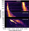 |
Fig. 1. Composite dynamic spectrum showing the evolution of the type II radio burst observed on 2022 May 19. The spectrum combines observations from three instruments: ORFEES (300−800 MHz), LOFAR HBA (110−240 MHz), and LOFAR LBA (30−88 MHz). The event starts at 12:02 UT with a single emission lane at frequencies around 600 MHz and drifts to lower frequencies. The top-right inset shows a zoomed-in view of the region where the single/double lane begins to evolve into a multilane structure. The multilane structure becomes particularly evident in the LOFAR LBA frequency range (30−88 MHz) after 12:08 UT. Note that F and H emissions are superposed at high frequencies, and in the LBA range they are distinct. The frequency range is plotted on a logarithmic scale to better display the fine structures across the wide frequency range. |
The type II burst started at 12:02 UT with emission observed at frequencies around 600 MHz, drifting to lower frequencies over time. At high frequencies (> 200 MHz), the F and H emission bands appear superposed, while they become clearly separated in the LOFAR LBA frequency range. The event initially shows a single/double lane structure at higher frequencies, but evolves into a complex multilane pattern. The onset of this transition is highlighted in the top-right inset of Fig. 1. The multilane structure is then particularly evident in the LOFAR LBA range (30−88 MHz) after 12:08 UT.
Similarly, as the spectrum also the radio imaging show an evolution of the complexity of the radio source location with time. Initially, a single radio source is identified along the shock front. Figure 2 presents the Solar Dynamics Observatory (SDO) Atmospheric Imaging Assembly (AIA; Lemen et al. 2012) running difference images at 193 Å, showing the CME eruption, with superposed Nançay Radioheliograph (NRH; Kerdraon & Delouis 1997) radio contours at 432 MHz, with one second integration time. The NRH data were processed using the standard SolarSoft (SSW) IDL package available in the SSW/radio/nrh directory, which includes routines for amplitude and phase calibration using the quiet Sun as reference (Mercier et al. 2015). The NRH observations at high frequencies show a single radio source location associated with the type II and the erupting CME front. This was also found by Vasanth et al. (2025), who present a single source for the NRH sources.
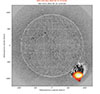 |
Fig. 2. Composite image showing the CME eruption observed on 2022 May 19. The background shows the SDO/AIA running difference image at 193 Å, revealing the CME front structure. The radio contours (in yellow and red) from NRH at 432 MHz show a single radio source location associated with the type II radio burst and the erupting CME front at 12:04 UT. The radio source at high frequencies appears as a single emission region, in contrast to the multiple emission regions observed at lower frequencies with LOFAR. |
LOFAR was observing in imaging mode only with the LBA range. The LBA frequency range (30−88 MHz) is particularly suitable for this analysis as the F and H emission bands are clearly separated, allowing us to independently study their source locations and evolution. The availability of interferometric imaging at these frequencies enables us to track the position and development of each emission lane throughout the event. The imaging in this work is performed with a combination of the core and remote stations of LOFAR. Radio imaging allows for arcminute-scale spatial resolution in decameter wavelength (Zhang et al. 2022; Morosan et al. 2025b). The LOFAR interferometry data processing consists of several sequential steps. First, we performed gain calibration by applying DP3 (Default Pre-Processing Pipeline2; van Diepen et al. 2018) to the Cas-A calibrator data to compute phase and amplitude offsets, using a flux density model as a reference. This generated gain solutions for each antenna and at each subband.
Following this, we inspected the antenna by examining phase and amplitude plots for each antenna to identify and flag corrupt data. The next step involved applying calibration corrections to phase and amplitude in the target observation using the gain solutions from DP3. For imaging, we transformed visibility data from wave vector space [u, v] to image space [x, y] using a 2D Fourier transform, employing the w-stacking CLEAN algorithm with wsclean for point-spread-function deconvolution3 (Offringa et al. 2014). Finally, in post-processing, we transformed coordinates to helio-projective and converted units to brightness temperature for further analysis using lofarSun4 (Zhang et al. 2022).
The LOFAR LBA interferometric data were also independently calibrated and imaged using the recently developed automated and self-calibration based pipeline – Solar IMaging Pipeline for LOFAR (SIMPL; Dey et al. 2025). Briefly, a quiet calibrator time window was identified for calibration. The amplitude component of the complex antenna gains estimated from the calibrator (Cas-A) was applied to the solar measurement sets. This was followed by self-calibration of solar datasets, with progressive baseline inclusion to gradually increase the model complexity. Once self-calibration converged, uv-based flagging was performed on the solar datasets in the CORRECTED_DATA column, independently for each time, frequency, and correlation (XX and YY). Beam correction toward the direction of the Sun was then applied, and spectroscopic snapshot images were produced using WSClean (Offringa et al. 2014). SIMPL provides a high dynamic range and improved image fidelity, even below 40 MHz, and the resulting spectroscopic snapshot images were used in the comparison of F and H emissions (discussed in Sect. 3).
To describe the observation of this complex type II event, we imaged each lane of the type II burst identified in the dynamic spectrum in the LOFAR LBA frequency range (30−88 MHz). Figure 3 shows an overview of the lanes observed with LOFAR LBA. The top panel presents the dynamic spectrum with seven selected lanes (including a quiet period), corresponding to different emission features observed during the event. The F plasma emission is represented by the type II lanes labeled 1 and 4, H emission is marked with lanes 2, 3, and 5, region 6 corresponds to a period of quiet emission, and 7a–c show the H emission appearing later in the event as three distinct parallel lanes. The top-right panel of Fig. 3 shows a zoomed-in view of the dynamic spectrum during an unusual phase of the event. We highlight region 3, where a third emission source begins to appear in both the spectrum and the corresponding radio imaging. This marks a transition from the initial double-source structure to a more complex configuration with three distinct emission regions; the imaging of this transition is shown in panels marked with 2 and 3 in Fig. 3. The lower panels of Fig. 3 present the LOFAR interferometric images corresponding to regions 1–6. The emission lanes (1–5) show an evolution in their spatial distribution: lanes 1–3 exhibit similar source locations with double source structures on the western and southern sides of the shock front; the size of the contour indicates the brightness temperature, which is reported in the white text in the bottom-left of each panel. Lane 4 shows emission predominantly on the western side, while lane 5 displays complex structures in both western and southern regions. Lane 6, corresponding to a period of reduced emission in the spectrum, shows brightness temperature levels comparable to the quiet Sun. The three parallel H lanes (7a–c), appearing later in the event, are presented in detail in Figs. 4 and 5, where their distinct spatial separation perpendicular to the shock propagation direction becomes evident. To accompany Fig. 3, we provide an overview online with the evolution of the event at 37.88 MHz, 54.49 MHz, 68.55 MHz, and 76.95 MHz.
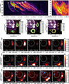 |
Fig. 3. Overview of the type II radio burst lanes observed with LOFAR LBA. Top-left panel: Dynamic spectrum in the frequency range 30−88 MHz. Seven different lanes along the radio burst are numbered, and a series of green points indicate the frequency and times of the observations presented in the lower panels. Lanes 1 and 2 show the initial double source structure, while region 3 marks the appearance of a third distinct emission source. These lanes are plotted with the relative EUV running difference emission to put the radio source in context with the driving front. Lower panels: LOFAR radio imaging of lanes 1–6, showing the spatial distribution of each emission feature. In the top row, the contours of the radio sources are color-coded by frequency (see the legend). The contours represent a brightness temperature of 15 MK for lane 1 and 120 MK for lanes 2 and 3. Lanes 4 and 5 show emission with varying spatial distributions. Lane 6 shows emission comparable to the quiet-Sun level. Lanes 7a–c, appearing later in time, represent harmonic emission and are parallel. Lanes 1 and 2 show similar source locations, with double source structures on the western and southern sides of the shock front. Lane 3 shows the moment where the third source starts to appear; the top-right panel shows a zoomed-in view of the spectrum at this moment, with the appearance of other lanes in the spectrum and the presence of a third source in the imaging. Lane 4 shows emission predominantly on the western side, while lane 5 exhibits complex structures in both the western and southern regions. Detailed imaging of the three parallel harmonic lanes 7a–c is presented in Figs. 4 and 5. |
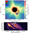 |
Fig. 4. Top: LOFAR radio imaging of the multilane structure in the type II radio burst. The background color map shows the electron density in the corona, as derived from the Predictive Science MHD model (Riley et al. 2011). Higher densities are in red, intermediate densities in green, and lower densities in blue. Bottom: Dynamic spectrum. The three observed lanes (blue, green, and red) are highlighted. The time of the radio imaging is indicated by the black squares (12:16 UT). LOFAR radio contours (80% level) for each lane are displayed in their respective colors, and the source centroid for each is marked with a colored point at the center of the corresponding contour. This figure highlights the correspondence between the radio multilane emission and the underlying coronal density structure. |
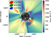 |
Fig. 5. LOFAR radio imaging of the multilane structure, over a background color map representing the coronal Alfvén speed from the Predictive Science MHD model (Riley et al. 2011). Radio contours (80% level) and centroids are shown as in Fig. 4. The dynamic spectrum and lane colors (blue, green, and red) match those in the previous figure. Notably, the central (red) radio source is located in a region of higher Alfvén speed. |
3. Results
The imaging analysis of this type II radio burst reveals several key features that evolve with time. Initially, at high frequencies (> 200 MHz), we observe a single radio source associated with the CME front, as shown by the NRH observations (Fig. 2). However, as the event progresses to lower frequencies, the radio emission becomes increasingly complex, revealing multiple distinct source regions.
In the LOFAR LBA frequency range (30−88 MHz), we identify seven distinct emission features (Fig. 3). Lanes 1–3 show emission with similar source locations, characterized by double source structures positioned on the western and southern sides of the shock front, above the EUV front observed in the Solar Ultraviolet Imager onboard GOES (SUVI). During this phase, we observe the emergence of a third distinct emission source. Lane 4 exhibits F emission predominantly localized to the western side of the shock front, while Lane 5 shows more complex H emission structures distributed across both western and southern regions. Lane 6 represents a transition period where the emission intensity becomes comparable to the quiet-Sun level, displaying complex spatial structures. The most notable feature appears in region 7, which splits into three parallel lanes (7a–c) in the H emission band. These lanes show clear spatial separation perpendicular to the shock propagation direction (radial), a feature not previously observed in type II bursts at these frequencies.
The comparison between the LOFAR-imaged radio source locations and the coronal parameters from the Predictive Science MAS magnetohydrodynamic (MHD) model (Riley et al. 2011) provides key insights into the physical conditions driving the multilane emission. The three parallel H lanes (7a–c) exhibit a clear one-to-one correspondence between their frequency drift rates and the local plasma densities at their respective source regions.
As shown in Fig. 4, we selected a representative time, midpoint along the lifetime of lanes 7a–c (12:16 UT), to best illustrate their spatial separation. At this moment, LOFAR LBA interferometric images (contours at the 80% brightness level) are overlaid on the electron-density distribution from the MAS MHD model. Each emission lane is marked in the dynamic-spectrum color (blue, green, and red), with the centroid positions marked. The red-lane source lies in a region of comparatively low density, producing the lowest-frequency emission; the blue source originates in a denser region, consistent with its higher-frequency lane; and the green source is located in an intermediate-density region, marking the middle-frequency lane. This spatial–spectral correspondence demonstrates that the multilane structure directly maps the coronal density stratification along separate parts of the CME-driven shock front.
Figure 5 presents the corresponding Alfvén-speed distribution from the same MHD model, again at 12:16 UT. The same LOFAR contours (80% level) and centroids are overlaid, preserving the color coding of the dynamic spectrum. The central (red) source coincides with a region of enhanced Alfvén speed, explaining its later appearance compared to the flank sources: in such regions, shock formation and particle acceleration are less efficient. Conversely, the blue and green flank sources lie in areas of lower Alfvén speed, favoring earlier shock formation and earlier-onset radio emission. This map–spectrum pairing further supports the interpretation that spatial variations in both plasma density and Alfvén speed control the timing and frequency characteristics of the observed multilane type II burst.
The spatial relationship between the F and H emission in type II solar radio bursts offers crucial insights into plasma emission mechanisms and the coronal environment. In this event, as shown in Fig. 6, LOFAR imaging enables a direct comparison of the F and H source locations for two distinct F–H pairs. Our analysis finds the F and H sources are largely co-spatial within the imaging and propagation limits, in agreement with several previous studies (e.g., Mann & Klassen 2005; Vršnak et al. 2001; McLean 1967). This observational result supports classical plasma emission models in which F and H originate from the same electron acceleration region. The online provided as supplementary material demonstrates this correlation persists dynamically throughout the evolution of the event.
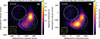 |
Fig. 6. LOFAR images showing the locations of F and H emission sources for two F–H pairs. The white contours, drawn at 0.1, 0.3, 0.5, 0.7, and 0.9 of the peak brightness temperature, represent the F emission, while the colored intensity (displayed with a square-root color scale, as indicated in the colorbar) corresponds to the H emission. The optical solar disk is shown as a dashed white circle. The white and yellow ellipses in the bottom-left corners indicate the restoring beams for the F and H maps, respectively. In both pairs, the F and H centroids are co-spatial within the LOFAR beam; however, the H emission is clearly resolved into two distinct components, whereas the F appears more extended and blended, likely due to the lower spatial resolution and stronger propagation effects at the F frequency. |
Figure 6 presents direct interferometric images of the two selected F–H pairs. The contours illustrate that while the centroids of the F and H sources are generally coincident within the LOFAR beam, the H band clearly resolves into two discrete components, in contrast to the more extended and blended appearance of the F emission.
A notable feature in our event is that, for both F–H source pairs, the H emission is resolved into two distinct sources, while the F emission remains more extended and appears as a single, broader region. This may result from the intrinsically larger beam at F frequencies and the greater influence of radio wave scattering and propagation (e.g., refractive spreading, ducting) at lower frequencies (Kontar et al. 2017). Such propagation effects can further blur the F emission, concealing double-source features that remain visible in the H band, in line with theoretical predictions and simulations of wave propagation in an inhomogeneous corona.
Our analysis reinforces the view that, while resolution and propagation effects can obscure finer structure at the F frequency, the origin sites of F and H emission in type II bursts are co-spatial to within observational limits. This is important for interpreting both the spectral and spatial features of type II radio bursts in the era of high-resolution, low-frequency solar imaging.
4. Conclusion and discussion
This study provides a detailed view of the spatial and spectral evolution of a complex, multilane type II solar radio burst associated with a CME-driven shock observed on 2022 May 19. Employing high-resolution LOFAR radio imaging in conjunction with coronal density and Alfvén speed modeling, we tracked the separation and progression of individual emission lanes and established their connection to specific regions along the shock front. This approach builds on previous studies of CME-related shocks and radio imaging (e.g., Zucca et al. 2014, 2018; Kong et al. 2012; Morosan et al. 2025a; Normo et al. 2025).
Our findings reveal a close correspondence between the dynamic spectrum and the spatial distribution of radio sources: the burst evolved from an initial single/double emission lane to multiple distinct spatial regions, culminating in a triple-lane configuration at low frequencies. Notably, each of these lanes maps to a region of distinct plasma density and local Alfvén speed. The occurrence of separate radio sources along different flanks and the apex of the shock supports the scenario that varying ambient coronal conditions govern the onset and spectral properties of type II emissions, with the spectral complexity reflecting coronal inhomogeneity. Recent findings of Feng & Zucca (2025), based on observations by the newly built Daocheng Solar Radio Telescope (DSRT), show that multilane structures often trace back to emission at physically separated sites along a curved shock front.
While our findings do not rule out other mechanisms for band-splitting or multiple lanes in type II bursts, such as upstream/downstream shock emission (Vršnak et al. 2001, 2002), they provide compelling evidence that, in this event, the multilane structure directly reflects the existence of spatially separated acceleration regions. The observed correspondence between lane frequencies and source locations, as well as between onset times and local Alfvén speeds, strongly supports this interpretation.
An additional key result of this work is the direct imaging of F and H source pairs (Sect. 3). Our LOFAR imaging (see Fig. 6) shows that the F and H sources are largely co-spatial, in agreement with previous studies (e.g., Mann & Klassen 2005). This observational result supports classical plasma emission models in which the two components originate from the same electron acceleration region. However, while the F emission appears as a single, broader region likely influenced by the larger LOFAR beam and propagation effects (such as refractive scattering and ducting) at F frequencies (Kontar et al. 2017), the H band clearly resolves into two discrete sources. This distinction highlights how both spatial resolution and radio wave propagation effects can influence the observed burst morphology and should be taken into consideration when interpreting multilane type II source structure.
Our work demonstrates the importance of advanced spectro-imaging techniques, such as those provided by LOFAR, in resolving the fine-scale structure of coronal-shock-related radio bursts. With the current upgrade of LOFAR 2.0 (LOFAR2.0 White Paper 2023), we will be able to perform imaging with LBA and HBA simultaneously. Continued observations at high spatial resolution, integrated with coronal modeling, will be crucial for disentangling the interplay between density, magnetic field, and shock geometry in solar radio burst generation.
Data availability
Supplementary movie 1 shows the evolution of the radio emission at four different frequencies throughout the event. Supplementary movie 2 shows the evolution of the F–H pair positions throughout the event. Movies are available at https://www.aanda.org
Acknowledgments
This paper is based on data obtained with the International LOFAR Telescope (ILT) under project code LT16-001 with PI Dr. P. Zucca. LOFAR (van Haarlem et al. 2013) is the Low Frequency Array designed and constructed by ASTRON. It has observing, data processing, and data storage facilities in several countries, that are owned by various parties (each with their own funding sources), and that are collectively operated by the ILT foundation under a joint scientific policy. The ILT resources have benefited from the following recent major funding sources: CNRS-INSU, Observatoire de Paris and Université d’Orléans, France; BMBF, MIWF-NRW, MPG, Germany; Science Foundation Ireland (SFI), Department of Business, Enterprise and Innovation (DBEI), Ireland; NWO, The Netherlands; The Science and Technology Facilities Council, UK; Polish Ministry of Science and Higher Education number: 2021/WK/2. KK acknowledges support by the Bulgarian National Science Fund, VIHREN program, under contract KP-06-DV-8/18.12.2019 (MOSAIICS project), as well as support from the LOFAR-BG project of the National Roadmap for Research Infrastructure of Bulgaria under contract D 01-110/30.06.2025. AK acknowledges the ANRF Prime Minister Early Career Research Grant (PM ECRG) program. D.E.M. acknowledges the Research Council of Finland project ‘SolShocks’ (grant number 354409). MN acknowledges support by the project “The Origin and Evolution of Solar Energetic Particles”, funded by the European Office of Aerospace Research and Development under award No. FA8655-24-1-7392. P.Z. acknowledges support for this research by the NASA Living with a Star Jack Eddy Postdoctoral Fellowship Program, administered by UCAR’s Cooperative Programs for the Advancement of Earth System Science (CPAESS) under award 80NSSC22M0097. S.D. acknowledges support from the Department of Atomic Energy, under project 12-R&D-TFR-5.02-0700. SDO data are courtesy of NASA/SDO and the AIA science teams. SUVI data are courtesy of NOAA/NESDIS/NCEI. The authors thank the Predictive Science team (https://www.predsci.com/) for making their MHD simulation results available. The authors would like to thank the radio observatory of Nançay for making the NRH and ORFEES data available. This research used the SunPy open source software package (The SunPy Community 2020). We thank the project LOFAR Data Valorization (LDV) [project numbers 2020.031, 2022.033, and 2024.047] of the research programme Computing Time on National Computer Facilities using SPIDER that is (co-)funded by the Dutch Research Council (NWO), hosted by SURF through the call for proposals of Computing Time on National Computer Facilities. We also thank SURF SARA with the project EINF-13633, Science ready products for LOFAR Solar, Heliospheric and ionospheric datasets.
References
- Alissandrakis, C. E. 2020, Front. Astron. Space Sci., 7, 74 [NASA ADS] [CrossRef] [Google Scholar]
- Bhunia, S., Carley, E. P., Oberoi, D., & Gallagher, P. T. 2023, A&A, 670, A169 [NASA ADS] [CrossRef] [EDP Sciences] [Google Scholar]
- Chen, B., Yu, S., Reeves, K. K., & Gary, D. E. 2018, Nat. Astron., 2, 1 [Google Scholar]
- Dey, S., Oberoi, D., Zucca, P., et al. 2025, A&A, in press, https://doi.org/10.1051/0004-6361/202556857 [Google Scholar]
- Dresing, N., Theesen, S., Klassen, A., & Gómez-Herrero, R. 2022, ApJ, 927, 1 [NASA ADS] [CrossRef] [Google Scholar]
- Eselevich, V., Eselevich, M., & Zimovets, I. 2013, Astron. Rep., 57, 142 [Google Scholar]
- Feng, S., & Zucca, P. 2025, Sol. Phys., 300, 108 [Google Scholar]
- Gopalswamy, N., Mäkelä, P., & Yashiro, S. 2016, ApJ, 819, L11 [Google Scholar]
- Hamini, A., Auxepaules, G., Birée, L., et al. 2021, J. Space Weather Space Clim., 11, 57 [NASA ADS] [CrossRef] [EDP Sciences] [Google Scholar]
- Kandekar, J., & Kumari, A. 2025, A&A, 697, L9 [NASA ADS] [CrossRef] [EDP Sciences] [Google Scholar]
- Kerdraon, A., & Delouis, J.-M. 1997, Coronal Physics from Radio and Space Observations (Springer), 192 [Google Scholar]
- Kong, X. L., Chen, Y., Li, G., et al. 2012, ApJ, 750, 158 [NASA ADS] [CrossRef] [Google Scholar]
- Kontar, E. P., Yu, S., Kuznetsov, A. A., et al. 2017, Nat. Commun., 8, 1515 [NASA ADS] [CrossRef] [Google Scholar]
- Kumari, A., Morosan, D. E., Kilpua, E. K. J., & Daei, F. 2023, A&A, 675, A102 [NASA ADS] [CrossRef] [EDP Sciences] [Google Scholar]
- Kumari, A., Morosan, D. E., Mugundhan, V., et al. 2025, A&A, 700, A274 [NASA ADS] [CrossRef] [EDP Sciences] [Google Scholar]
- Lemen, J. R., Title, A. M., Akin, D. J., et al. 2012, Sol. Phys., 275, 17 [Google Scholar]
- LOFAR2.0 White Paper 2023, LOFAR2.0 White Paper – v2023.1: A Premier Low-Frequency Radio Telescope for the 2020s, Tech. Rep., International LOFAR Telescope (ILT), first printing, April 2023 [Google Scholar]
- Magdalenić, J., Marqué, C., Zhukov, A. N., Vršnak, B., & Veronig, A. 2012, Sol. Phys., 280, 551 [NASA ADS] [CrossRef] [Google Scholar]
- Maguire, C. A., Carley, E. P., McCauley, J., et al. 2020, A&A, 633, A56 [NASA ADS] [CrossRef] [EDP Sciences] [Google Scholar]
- Maguire, C. A., Carley, E. P., Zucca, P., Vilmer, N., & Gallagher, P. T. 2021, ApJ, 909, 2 [NASA ADS] [CrossRef] [Google Scholar]
- Mann, G., & Klassen, A. 2005, A&A, 441, 319 [NASA ADS] [CrossRef] [EDP Sciences] [Google Scholar]
- McLean, D. J. 1967, PASA, 1, 47 [Google Scholar]
- Mercier, C., Chambe, G., & Kerdraon, A. 2015, A&A, 583, A101 [NASA ADS] [CrossRef] [EDP Sciences] [Google Scholar]
- Morosan, D. E., Carley, E. P., Hayes, L. A., et al. 2019, Nat. Astron., 3, 452 [Google Scholar]
- Morosan, D. E., Dresing, N., Palmroos, C., et al. 2025a, A&A, 693, A296 [NASA ADS] [CrossRef] [EDP Sciences] [Google Scholar]
- Morosan, D. E., Jebaraj, I. C., Zhang, P., et al. 2025b, A&A, 695, A70 [NASA ADS] [CrossRef] [EDP Sciences] [Google Scholar]
- Normo, S., Morosan, D. E., Zhang, P., Zucca, P., & Vainio, R. 2025, A&A, 698, A175 [NASA ADS] [CrossRef] [EDP Sciences] [Google Scholar]
- Offringa, A. R., McKinley, B., Hurley-Walker, N., et al. 2014, MNRAS, 444, 606 [Google Scholar]
- Ramesh, R., Kathiravan, C., & Kumari, A. 2023, ApJ, 943, 43 [NASA ADS] [CrossRef] [Google Scholar]
- Riley, P., Lionello, R., Linker, J. A., & Mikic, Z. 2011, Sol. Phys., 274, 361 [NASA ADS] [CrossRef] [Google Scholar]
- Smerd, S. F., Sheridan, K. V., & Stewart, R. T. 1974, Coronal Disturbances (Dordrecht: Springer), 389 [Google Scholar]
- Smerd, S. F., Sheridan, K. V., & Stewart, R. T. 1975, ApJ, 16, 23 [Google Scholar]
- Sturrock, P. A. 1961, Nature, 192, 58 [Google Scholar]
- The SunPy Community (Barnes, W. T., et al.) 2020, ApJ, 890, 68 [Google Scholar]
- van Diepen, G., Dijkema, T. J., & Offringa, A. 2018, Astrophysics Source Code Library [record ascl:1804.003] [Google Scholar]
- van Haarlem, M. P., Wise, M. W., Gunst, A., et al. 2013, A&A, 556, A2 [NASA ADS] [CrossRef] [EDP Sciences] [Google Scholar]
- Vasanth, V., Chen, Y., & Michalek, G. 2025, A&A, 702, A15 [NASA ADS] [CrossRef] [EDP Sciences] [Google Scholar]
- Vršnak, B., Aurass, H., Magdalenić, J., & Mann, G. 2001, A&A, 377, 321 [NASA ADS] [CrossRef] [EDP Sciences] [Google Scholar]
- Vršnak, B., Magdalenić, J., Aurass, H., & Mann, G. 2002, A&A, 396, 673 [NASA ADS] [CrossRef] [EDP Sciences] [Google Scholar]
- Wild, J. P., & McCready, L. L. 1950, Aust. J. Sci. Res. A Phys. Sci., 3, 387 [Google Scholar]
- Zhang, P., Zucca, P., Kozarev, K., et al. 2022, ApJ, 932, 17 [CrossRef] [Google Scholar]
- Zhang, P., Offringa, A. R., Zucca, P., Kozarev, K., & Mancini, M. 2023, MNRAS, 521, 630 [NASA ADS] [CrossRef] [Google Scholar]
- Zimovets, I. V. 2012, Sol. Phys., 280, 563 [Google Scholar]
- Zimovets, I. V., & Sadykov, V. M. 2015, Adv. Space Res., 56, 2811 [NASA ADS] [CrossRef] [Google Scholar]
- Zucca, P., Carley, E. P., Bloomfield, D. S., & Gallagher, P. T. 2014, A&A, 564, A47 [NASA ADS] [CrossRef] [EDP Sciences] [Google Scholar]
- Zucca, P., Morosan, D. E., Rouillard, A. P., et al. 2018, A&A, 615, A89 [NASA ADS] [CrossRef] [EDP Sciences] [Google Scholar]
All Figures
|
Fig. 1. Composite dynamic spectrum showing the evolution of the type II radio burst observed on 2022 May 19. The spectrum combines observations from three instruments: ORFEES (300−800 MHz), LOFAR HBA (110−240 MHz), and LOFAR LBA (30−88 MHz). The event starts at 12:02 UT with a single emission lane at frequencies around 600 MHz and drifts to lower frequencies. The top-right inset shows a zoomed-in view of the region where the single/double lane begins to evolve into a multilane structure. The multilane structure becomes particularly evident in the LOFAR LBA frequency range (30−88 MHz) after 12:08 UT. Note that F and H emissions are superposed at high frequencies, and in the LBA range they are distinct. The frequency range is plotted on a logarithmic scale to better display the fine structures across the wide frequency range. |
| In the text | |
|
Fig. 2. Composite image showing the CME eruption observed on 2022 May 19. The background shows the SDO/AIA running difference image at 193 Å, revealing the CME front structure. The radio contours (in yellow and red) from NRH at 432 MHz show a single radio source location associated with the type II radio burst and the erupting CME front at 12:04 UT. The radio source at high frequencies appears as a single emission region, in contrast to the multiple emission regions observed at lower frequencies with LOFAR. |
| In the text | |
|
Fig. 3. Overview of the type II radio burst lanes observed with LOFAR LBA. Top-left panel: Dynamic spectrum in the frequency range 30−88 MHz. Seven different lanes along the radio burst are numbered, and a series of green points indicate the frequency and times of the observations presented in the lower panels. Lanes 1 and 2 show the initial double source structure, while region 3 marks the appearance of a third distinct emission source. These lanes are plotted with the relative EUV running difference emission to put the radio source in context with the driving front. Lower panels: LOFAR radio imaging of lanes 1–6, showing the spatial distribution of each emission feature. In the top row, the contours of the radio sources are color-coded by frequency (see the legend). The contours represent a brightness temperature of 15 MK for lane 1 and 120 MK for lanes 2 and 3. Lanes 4 and 5 show emission with varying spatial distributions. Lane 6 shows emission comparable to the quiet-Sun level. Lanes 7a–c, appearing later in time, represent harmonic emission and are parallel. Lanes 1 and 2 show similar source locations, with double source structures on the western and southern sides of the shock front. Lane 3 shows the moment where the third source starts to appear; the top-right panel shows a zoomed-in view of the spectrum at this moment, with the appearance of other lanes in the spectrum and the presence of a third source in the imaging. Lane 4 shows emission predominantly on the western side, while lane 5 exhibits complex structures in both the western and southern regions. Detailed imaging of the three parallel harmonic lanes 7a–c is presented in Figs. 4 and 5. |
| In the text | |
|
Fig. 4. Top: LOFAR radio imaging of the multilane structure in the type II radio burst. The background color map shows the electron density in the corona, as derived from the Predictive Science MHD model (Riley et al. 2011). Higher densities are in red, intermediate densities in green, and lower densities in blue. Bottom: Dynamic spectrum. The three observed lanes (blue, green, and red) are highlighted. The time of the radio imaging is indicated by the black squares (12:16 UT). LOFAR radio contours (80% level) for each lane are displayed in their respective colors, and the source centroid for each is marked with a colored point at the center of the corresponding contour. This figure highlights the correspondence between the radio multilane emission and the underlying coronal density structure. |
| In the text | |
|
Fig. 5. LOFAR radio imaging of the multilane structure, over a background color map representing the coronal Alfvén speed from the Predictive Science MHD model (Riley et al. 2011). Radio contours (80% level) and centroids are shown as in Fig. 4. The dynamic spectrum and lane colors (blue, green, and red) match those in the previous figure. Notably, the central (red) radio source is located in a region of higher Alfvén speed. |
| In the text | |
|
Fig. 6. LOFAR images showing the locations of F and H emission sources for two F–H pairs. The white contours, drawn at 0.1, 0.3, 0.5, 0.7, and 0.9 of the peak brightness temperature, represent the F emission, while the colored intensity (displayed with a square-root color scale, as indicated in the colorbar) corresponds to the H emission. The optical solar disk is shown as a dashed white circle. The white and yellow ellipses in the bottom-left corners indicate the restoring beams for the F and H maps, respectively. In both pairs, the F and H centroids are co-spatial within the LOFAR beam; however, the H emission is clearly resolved into two distinct components, whereas the F appears more extended and blended, likely due to the lower spatial resolution and stronger propagation effects at the F frequency. |
| In the text | |
Current usage metrics show cumulative count of Article Views (full-text article views including HTML views, PDF and ePub downloads, according to the available data) and Abstracts Views on Vision4Press platform.
Data correspond to usage on the plateform after 2015. The current usage metrics is available 48-96 hours after online publication and is updated daily on week days.
Initial download of the metrics may take a while.