| Issue |
A&A
Volume 703, November 2025
|
|
|---|---|---|
| Article Number | A137 | |
| Number of page(s) | 11 | |
| Section | Astrophysical processes | |
| DOI | https://doi.org/10.1051/0004-6361/202554508 | |
| Published online | 13 November 2025 | |
Retrieving the hot circumgalactic medium physics from the X-ray radial profile from eROSITA with an IlustrisTNG-based forward model
1
Max Planck Institute for Extraterrestrial Physics (MPE), Gießenbachstraße 1, 85748 Garching, Munich, Germany
2
INAF-Osservatorio Astronomico di Brera, Via E. Bianchi 46, I-23807 Merate, (LC), Italy
3
Como Lake Center for Astrophysics (CLAP), DiSAT, Università degli Studi dell’Insubria, Via Valleggio 11, I-22100 Como, Italy
4
European Southern Observatory, Karl-Schwarzschild-Straße 2, 85748 Garching, Munich, Germany
5
Exzellenzcluster ORIGINS, Boltzmannstr. 2, 85748 Garching, Germany
⋆ Corresponding author: This email address is being protected from spambots. You need JavaScript enabled to view it.
Received:
13
March
2025
Accepted:
8
September
2025
Abstract
Aims. Recent eROSITA measurements of the radial profiles of the hot circumgalactic medium (CGM) in the Milky Way stellar mass (MW-mass) regime provide us with a new benchmark to constrain the hot gas around MW-mass central and satellite galaxies and their halo mass distributions. Modeling this rich data set with state-of-the-art hydrodynamical simulations is required to further our understanding of the shortcomings in the current paradigm of galaxy formation and evolution models.
Methods. We developed forward models for the stacked X-ray radial surface brightness profile measured by eROSITA around MW-mass galaxies. Our model contains two emitting components: hot gas (around central galaxies and around satellite galaxies hosted by more massive halos) and X-ray point sources (X-ray binaries (XRBs) and active galactic nuclei (AGNs)). We modeled the hot gas profile using the TNG300-based products. We generated mock observations with our TNG300-based model (matching stellar mass and redshift with observations) with different underlying halo mass distributions. Therefore, we tested the CGM properties as a function of their host halo mass distribution. The point sources are described by a simple point spread function of eROSITA, and we fit their normalization in this work. In total, we fit the X-ray surface brightness profile with two free parameters: the normalization of satellites in more massive host halos and the normalization of the mean point source emission.
Results. We show that for the same mean stellar mass, a factor ∼2× increase in the mean value of the underlying halo mass distribution results in ∼4× increase in the stacked X-ray luminosity from the hot CGM. Using empirical models to derive a permissible range of AGN and XRB luminosities in the MW-mass X-ray galaxy stack, we choose our forward model that best describes the hot CGM for the eROSITA observations. Our chosen model in the MW stellar mass bin is in good agreement with previous literature results. We find that at ≲40 kpc from the galaxy center, the hot CGM from central galaxies and the X-ray point sources emission (from XRBs and AGNs) each account for 40 − 50% of the total X-ray emission budget. Beyond ∼40 kpc, we find that the hot CGM around satellites (probing their more massive host halos with mean M200m ∼ 1014 M⊙) dominates the stacked X-ray surface brightness profile.
Conclusions. The gas physics driving the shape of the observed hot CGM (in stellar-mass-selected X-ray stacking experiments) is tightly correlated with the underlying halo-mass distribution. This work provides a novel technique to constrain the AGN X-ray luminosity jointly with the radial hot CGM gas distribution within the halo using measurements from X-ray galaxy stacking experiments. Implementing this technique on other state-of-the-art simulations will provide a new ground for testing different galaxy formation models with observations.
Key words: galaxies: evolution / galaxies: statistics / X-rays: galaxies / X-rays: general
© The Authors 2025
 Open Access article, published by EDP Sciences, under the terms of the Creative Commons Attribution License (https://creativecommons.org/licenses/by/4.0), which permits unrestricted use, distribution, and reproduction in any medium, provided the original work is properly cited.
This article is published in open access under the Subscribe to Open model.
Open access funding provided by Max Planck Society.
1. Introduction
The circumgalactic medium (CGM) plays a crucial role in a galaxy’s evolution by directly tracing inflows and outflows of gas driven by various gravitational and nongravitational mechanisms (see Faucher-Giguère & Oh 2023 for an overview). The nongravitational mechanisms, such as stellar and active galactic nucleus (AGN) feedback, heat and cool the gas, impacting the evolution of star formation in the galaxy (Donahue & Voit 2022). The relative contributions from shock heating of the gas due to gravitational infall, stellar, and AGN heating are model-dependent in the current paradigm of galaxy formation and evolution. Particularly, the impact of stellar and AGN feedback depends on the host halo mass, where the former affects the halo masses ≲1012 M⊙, and the latter affects the ≳1012 M⊙, respectively (Wechsler & Tinker 2018). The pivotal point, where the relative contributions from stellar and AGN feedback are equally important, occurs at halo mass scales similar to the one of our Milky Way (MW), defining it as a crucial testing range for the models.
The interplay between feedback mechanisms and the galactic atmosphere results in a multiphase CGM, with the hot phase (T ≳ 106 K) typically being the most massive and volume-filling component (see review by Tumlinson et al. 2017). The hot CGM radiates in the soft X-ray within the 0.2 − 2 keV energy band for MW-mass halos due to thermal hot gas emission. There are various techniques to probe the hot CGM in X-rays via absorption (Galeazzi et al. 2007; Bhattacharyya et al. 2023; Mathur et al. 2023; Wijers et al. 2020; Bogdán et al. 2023) and emission (Koutroumpa et al. 2007; Bertone et al. 2010; van de Voort 2013; Bogdán et al. 2013a,b, 2017; Anderson et al. 2016; Li et al. 2017; Das et al. 2019; Zhang et al. 2022; Ponti et al. 2023; Locatelli et al. 2024; Zheng et al. 2024). In particular, emission studies, combined with stacking, allow us to map the large-scale extent of the hot CGM to the halo’s virial radius (Anderson et al. 2015; Oppenheimer et al. 2020; Comparat et al. 2022; Chadayammuri et al. 2022; Zhang et al. 2024a).
Given the advent of eROSITA (Merloni et al. 2024), there have been several studies exploiting the unprecedented statistics for stacking the X-ray emission at the position of optically selected galaxies, such as Comparat et al. (2022), Chadayammuri et al. (2022), and most recently Zhang et al. (2024a, hereafter Z24). Z24 represent the state-of-the-art hot CGM measurements for MW-mass galaxies, given the largest optical galaxy sample with the German half-sky eROSITA coverage in X-rays. They stack 415 627 galaxies with photometric redshifts, Fullphot, from the DESI Legacy Survey DR 9 (Dey et al. 2019; Zou et al. 2019, 2022) and 30 825 central galaxies with spectroscopic redshifts from the SDSS DR7 Main Galaxy Sample (Strauss et al. 2002; Abazajian et al. 2009). The latter, the SDSS-based central galaxy sample, has the advantage of spectroscopic information, allowing for galaxies to be classified into centrals and satellites with halo mass information (Tinker 2021). Therefore, Z24 retrieve the X-ray surface brightness profile from the hot CGM by empirically modeling the impact due to satellites, AGNs, and XRB emissions. However, the former, the DESI Legacy survey-based galaxy sample, cannot be classified into centrals and satellites, given the limitations in photometric redshift, making the modeling of this dataset challenging. To exploit the highest signal-to-noise data (a factor of 13.5 times more statistics than the spectroscopic sample) to date, in this work, we embark on constructing a forward model to disentangle the hot CGM radial profiles from the X-ray stack of optically selected galaxies.
Among the dominating sources of contamination in X-ray stacking experiments at MW-mass galaxies are (1) the AGN and X-ray binary (XRB) population of galaxies (Biffi et al. 2018a; Vladutescu-Zopp et al. 2023), and (2) the effect of having satellite galaxies in the stacking sample, where these satellites contribute to the averaged X-ray stack with their more massive host galaxy within which they are embedded in the large-scale structure (see e.g., Shreeram et al. 2025; Weng et al. 2024). Given that we are modeling a photometric galaxy sample in this work, we do not have the classification of galaxies into centrals and satellites due to limitations in the (photometric) redshift accuracy for the galaxies in large optical surveys. Therefore, we use our TNG-based forward model fit for the magnitude of the satellite galaxy contribution by setting the normalization of the surface brightness profile free when fitting to data. The contaminating effect of the satellites was quantified in detail in Shreeram et al. (2025), where we find that this effect becomes increasingly significant in the stacking sample as the stellar mass decreases. When conducting blind X-ray stacking analysis at the positions of optically selected galaxies, where centrals and satellites are unclassified, the inclusion of satellites implies that the total measured X-ray surface brightness profile comprises (i) the intrinsic hot gas emission around truly central galaxies and (ii) the contamination of hot gas emission measured around satellites. We emphasize that the latter does not correspond to the emission intrinsic to the satellites as the more massive host (central) galaxy in the vicinity of the satellite dominates the emission, resulting in a negligible contribution of the intrinsic satellite emission (see e.g., Rohr et al. 2024).
This paper presents a forward model for the stacked galaxy profile comprising the X-ray emitting gas and point source emission. We use the lightcone built with TNG300 in Shreeram et al. (2025) to construct mock galaxy catalogs representing the observations. From our TNG-based mock galaxy catalog, we predict the hot gas CGM profile contribution to the X-ray galaxy stack from central and satellite galaxies. We parameterize the normalization of the hot gas contribution from satellites, 𝒩sat. The hot gas prediction for central galaxies from our forward model with TNG is left unchanged. As for the point-like source contributions from AGNs and XRBs, we do not use the simulations, which are quite uncertain in their predicted instantaneous AGN activity, but instead we describe their contribution with a normalization parameter, 𝒩ps, and fix the radial shape using the point spread function (PSF) of eROSITA. This leaves us with two fitting parameters in our model: the contribution of point sources in the stack, 𝒩ps, and the normalization of the satellite X-ray surface brightness profile, 𝒩sat. We fit our forward model to the mean X-ray surface brightness profile reported Z24, obtained by stacking MW-mass galaxies. We obtain the point source luminosity from our fitting analysis, and we interpret our results by comparing them with independent empirical models of AGN luminosity functions.
The paper is organized as follows. Sect. 2 expands on the observational data used for modeling in this study. Sect. 3 describes the forward model built in this work; details on the point source and hot gas component are provided in Sects. 3.1 and 3.2, respectively, and details on the generation of mock galaxy catalogs in Sect. 3.3. Sect. 4 interprets and discusses the results, and Sect. 5 summarizes the main findings of this work.
2. Data
This study uses the results from Z24, where they use optical data from the Legacy Survey Data release 9 (Dey et al. 2019), and X-ray data from the first four SRG/eROSITA All-Sky Surveys (eRASS:4) within the western galactic hemisphere (Merloni et al. 2024). Here, we summarize the relevant details from Z24 to motivate the forward-model setup, as is described in Sect. 3.
The LS DR9 overlaps by 9340 deg2 with the western Galactic hemisphere. Z24 define the Fullphot sample containing 1 677 909 galaxies, which is based on the LS DR9 galaxy catalog from Zou et al. (2019, 2022), where they provide the galaxy properties. The stellar masses, M⋆, with uncertainties of ∼0.2 dex are provided in the range 9.5 < log M⋆ < 11.5 and the photometric redshifts, zphot, with uncertainty Δzphot ≲ 0.03, spans the range 0.01 < zphot < 0.4 (see Table 3 in Z24 for further classification into stellar mass bins). We focus here on the modeling of the X-ray emission from MW-like galaxies, defined by the stellar mass bin 10.5 < log10M⋆ < 11.0, and located in the redshift range 0.02 < zphot < 0.17; containing 415 627 galaxies and median stellar mass and redshift of 5.5 × 10¹⁰ M⊙ and zphot = 0.14, respectively.
The details on the data analysis pipeline to obtain the observed X-ray surface brightness profiles, based on the LS DR9 (Fullphot) galaxies, are provided in Z24. They stack the X-ray data in different stellar mass bins following the method from Comparat et al. (2022). The first step is to generate X-ray event cubes around every galaxy in the sample within 3 Mpc. The events within the cube are assigned a physical radial distance from the source, Rkpc, along with the exposure time, texp, effective collecting area, Aeff, and the rest frame energy of the event around the source, Erest. The X-ray surface brightness profile around the galaxy is obtained, with additional correction factors due to absorption and area loss if masking of sources is applied (see Eq. 1 in Z24). We use the background-subtracted profiles for modeling in this work (for details on the background treatment in the data, see Appendix A in Z24).
3. Forward model built in this work
This section explains the forward model we built to fit the observed X-ray surface brightness profile reported in Z24. The mean X-ray surface brightness profile obtained from X-ray stacking of galaxies on their optically detected positions is expressed as
 (1)
(1)
where SX, hot gas[r] is the X-ray contribution to SX, total(r) from hot gas (further detailed in Sect. 3.2) and SX, point − source[r] is the X-ray contribution from AGNs and XRBs (Sect. 3.1). We then introduce the forward models constructed in this work in Sect. 3.3.
3.1. The point source component
The SX, point − source[r] component is expressed as
 (2)
(2)
where 𝒩ps is the normalization of the point-source component and PSF[z, r] is the shape of the point-source component as defined by the survey-averaged eROSITA PSF. Here, the shape of the mean PSF was obtained by converting from angular to physical scale [kiloparsecs] using the redshifts of the galaxies in the stacking sample. We constrained 𝒩ps by fitting the observations.
We did not use the TNG300 outputs to predict the contributions from AGNs and XRBs for the following reasons. As is presented in Habouzit et al. (2019), the X-ray luminosity function (XLF) for AGNs in TNG shows an overproduction of faint AGNs at z = 0, a common problem in hydrodynamical cosmological simulations due to poorly resolved sub-grid feedback prescriptions (Sijacki et al. 2015; Volonteri et al. 2016; Rosas-Guevara et al. 2016; Biffi et al. 2018a). Additionally, in TNG, the bright end underpredicts the XLF compared with observations due to the over-efficient kinetic mode of feedback prescriptions with TNG (Habouzit et al. 2019). Given these discrepancies between the hydrodynamical simulations and observations, using the TNG-based predictions for the X-ray AGN contribution would be unreliable for the purpose of this work. As for XRBs, whose prediction depends on the star formation rates (SFRs) of galaxies (more details in Sect. 4.1), using the TNG SFR values for the mock galaxies to represent observations requires extreme care, given how sensitive the SFR is to the definition of quenched galaxies, the physical apertures used for measurement of the SFR, and the mass resolution of the simulation (Donnari et al. 2019). Additionally, the quenched fraction of satellite galaxies is overestimated in the stellar mass range of M⋆ ∈ 1010 − 11 M⊙ at z = 0 (Donnari et al. 2021), which entails the mass range of interest in this work. These caveats impede us from reliably predicting meaningful estimates for point source contributions intrinsic to the TNG model that can be directly compared with observations.
In this work, we use independent empirical estimates (Sects. 4.1 and 4.2) to predict the allowed range of the mean X-ray luminosity from XRBs and AGNs, respectively. Since the estimates from these empirical models are independent of TNG, we use them to inform our forward models for the permitted values of point source luminosities, as is shown in Fig. 2.
3.2. The hot gas component
In this work, we modeled the hot gas emission using the TNG300 hydrodynamical simulations (Pillepich et al. 2018; Marinacci et al. 2018; Naiman et al. 2018; Nelson et al. 2015; Springel et al. 2018); we used TNG300 to construct a lightcone and generate mock X-ray observations, as presented in Shreeram et al. (2025). Here, we summarize the most important features. We used the IllustrisTNG cosmological hydrodynamical simulation with the box of side length 302.6 Mpc (Nelson et al. 2019, TNG300)1; this box size allows us to map the hot CGM around MW-mass analogs embedded in the large-scale structure. TNG300 contains 25003 dark matter particles, with a baryonic mass resolution of 1.1 × 10⁷ M⊙ (resulting in ≳103 particles at MW-mass galaxies), a comoving value of the adaptive gas gravitational softening length for gas cells of 370 comoving parsec (allowing us to resolve the X-ray gas from ∼5 kpc from the halo center), gravitational softening of the collisionless component of 1.48 kpc, and dark matter mass resolution of 5.9 × 10⁷ M⊙. The TNG simulations adopt the Planck Collaboration XIII (2016) cosmological parameters. The TNG300 lightcone, LC-TNG300, was constructed with the box remap technique (Carlson & White 2010), using the LightGen code2. LC-TNG300 spans across redshifts 0.03 ≲ z ≲ 0.3; this range is motivated by observations (e.g., Comparat et al. 2022; Chadayammuri et al. 2022; Zhang et al. 2024a). It goes out to 1231 cMpc along the x axis, subtending an area of 47.28 deg2 on the sky in the y − z plane. The physical properties of the distinct halos and subhalos within the TNG300 lightcone are obtained by the SUBFIND algorithm (Springel et al. 2001; Dolag et al. 2009). SUBFIND detects gravitationally bound substructures, equivalent to galaxies in observations, and also provides us with a classification of subhalos into centrals and satellites, where centrals are the most massive substructure within a distinct halo. For the MW-mass bin3, M⋆ = 1010.5 − 11 M⊙, we have 5109 centrals and 2719 satellites, resulting in a total simulated galaxy catalog with 7828 galaxies (subhalos).
The X-ray photons were simulated within the LC-TNG300 in the 0.5 − 2.0 keV intrinsic band with pyXsim (ZuHone & Hallman 2016), which is based on PHOX (Biffi et al. 2013, 2018b), by assuming an input emission model where the hot X-ray emitting gas is in collisional ionization equilibrium. The spectral model computations of hot plasma use the Astrophysical Plasma Emission Code, APEC4 code (Smith et al. 2001) with atomic data from ATOMDB v3.0.9 (Foster et al. 2012). This model uses the plasma temperature of the gas cells (in keV), the redshift z, and metallicity; Shreeram et al. (2025) assume a constant metallicity of 0.3 Z⊙ for the generation of X-ray events. The X-ray events use the solar abundance values from Anders & Grevesse (1989). The events are generated by assuming a telescope with an energy-independent collecting area of 1000 cm2 and an exposure time of 1000 ks. The photon list is generated in the observed frame of the X-ray emitting gas cells and is corrected to rest frame energies. Finally, the photons generated by the gas cells are projected onto the sky.
We obtained X-ray radial surface brightness profiles in the 0.5 − 2.0 keV band for all galaxies. Given that SUBFIND provides us with an accurate classification of galaxies into centrals and satellites, we distinguish the hot gas component into X-ray emissions around centrals and satellites. For central galaxies, the profiles represent the hot gas emission around them; however, for satellite galaxies, the profiles probe the hot gas emission of the more massive host halo in the vicinity.
We convolved the individual X-ray surface brightness profiles from LC-TNG300-based mock galaxies catalogs with the eROSITA PSF (Merloni et al. 2024). The PSF convolved mean X-ray surface brightness profile from hot gas, SX, hot gas[r], is expressed as follows:
 (3)
(3)
where SX, cen is the TNG-based prediction for the hot gas around central galaxies and SX, sat corresponds to the hot gas around satellites. After matching LC-TNG300 with Fullphot in stellar mass and redshift, the mock galaxy catalogs fix the fraction of centrals, fcen, and satellites, fsat. 𝒩sat is the factor by which the mock prediction from SX, sat is rescaled to match the observations, thereby renormalizes the SX, sat of the TNG300-based prediction; 𝒩sat is the only free parameter in the hot gas emission component.
The motivation behind introducing the renormalization parameter, 𝒩sat, for fitting the forward model prediction for SX, sat with observations is as follows. The TNG-based prediction for SX, sat from the mock catalogs (for a given fsat) is ∼5 − 7× brighter than the Fullphot stack. Shreeram et al. (2025) find that the shape of the X-ray radial surface brightness profile from satellite galaxies (hosted by massive halos) is unaffected by fsat in the galaxy sample. This is because the halo masses making up the average profile from satellite galaxies, whose M⋆ ∈ 1010.5 − 11 M⊙, are dominated by host (central) halos with mean M200m ∼ 1014 M⊙. Therefore, by changing the normalization of the SX, sat, we effectively damp the normalization of the X-ray thermal gas contribution from the most massive clusters in the simulation. This is justified given that the hot gas fraction from TNG is overpredicted at halo masses above M500c ≳ 1013.5 M⊙, as shown in Fig. 6 in Popesso et al. (2024a). This is also reflected in the LX − M500c relation shown in Zhang et al. (2024b) and Popesso et al. (2024b).
We emphasize that the X-ray surface brightness profile prediction from central galaxies, SX, cen, which represents the CGM physics of interest in this work, is untouched. We predict multiple CGM profiles by changing the host halo mass distribution of the central galaxies and propagating it through our pipeline to generate mock galaxy catalogs for each halo distribution considered, as detailed in the following section. Note that the stellar mass and redshift distributions are the same for all three models.
We restricted our analysis to the MW-mass stellar bin due to both observational and modeling constraints. While comparisons across a broader stellar mass range are desirable, for lower-mass galaxies, there is currently no suitable X-ray stacking data available. For higher-mass galaxies, the existing stacked X-ray measurements (e.g., from Z24) extend to redshifts beyond the coverage of our lightcone, LC-TNG300, which is built from the TNG300 simulation. Extending the analysis to these massive galaxies would require constructing a new lightcone from a larger-volume simulation (e.g., FLAMINGO, MTNG), generating matched mock X-ray observations, and repeating the full forward-modeling pipeline introduced here, an effort that warrants a future study. In contrast, the MW-mass bin provides both observational data within the redshift range of LC-TNG300, making it the optimal case for robust model–data comparison and the hot CGM signal retrieval.
3.3. Mock galaxy catalogs
We next used the LC-TNG300 galaxy catalog to construct a mock galaxy sample for the LS DR9 Fullphot galaxies. We matched every one of the 415 627 galaxies in the Fullphot sample with a galaxy from LC-TNG300 in redshift and stellar mass. By construction, the simulated LC-TNG300 galaxies follow the same stellar mass and redshift distribution as the observational sample. The mock sample predicts the mean X-ray surface brightness profile for gas emitted around centrals and satellites.
In this work, we also tested the impact of the underlying halo mass distribution on the CGM physics. Therefore, we additionally generated two other mock galaxy catalogs using LC-TNG300, matched in stellar mass and redshift; however, with different underlying halo mass distributions (see left panel of Fig. 1). Consequently, we also emulated the corresponding X-ray surface brightness profiles by varying the halo distributions (see right panel of Fig. 1). The differences between the three forward models are as follows:
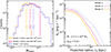 |
Fig. 1. Forward models constructed in this work for the hot CGM from central galaxies by varying the underlying halo mass distribution. Left panel: Purple halo mass distribution (Model 1) obtained from the mock central galaxy catalog – constructed with the TNG300 lightcone (LC-TNG300) from Shreeram et al. (2025) – for the X-ray stack from Z24 that uses optically detected galaxies with photometric redshifts (Fullphot) from LS DR9 (Dey et al. 2019). Note that the mock galaxy catalog is generated by matching LC-TNG300 to Fullphot in stellar mass and redshift (see details in Sect. 3.3); the median stellar mass and redshift of the Fullphot (and our mock catalogs) are 5.5 × 10¹⁰ M⊙ and 0.14, respectively. The underlying halo mass distribution of the Fullphot optical dataset is unknown. The pink distribution (Model 2; with mean M200m = 5.4 × 10¹² M⊙) discards the top 10% most massive halos before the generation of the mock galaxy catalog. The yellow distribution (Model 3; with mean M200m = 3.5 × 10¹² M⊙) discards the top 30% most massive halos before the generation of the mock galaxy catalog. Right panel: Corresponding X-ray surface brightness profiles in the 0.5 − 2 kev energy band (for details on their generation see Sect. 3.2) for the three mock galaxy catalogs with different halo mass distributions, which are shown in the left panel. The profiles are convolved with the eROSITA PSF, and they represent the Fullphot dataset in the stellar mass and redshift plane. Nevertheless, due to the impact of the underlying halo mass distribution, the shape and normalization of the hot CGM profiles are impacted, where discarding the most massive halos from the underlying halo distribution results in steeper profiles with lower normalizations. |
-
Model 1 leaves LC-TNG300 halo mass distribution unchanged (purple line in Fig. 2), resulting in the mean halo mass of M200m = 6.5 × 10¹² M⊙.
-
Model 2 changes the underlying central galaxy halo distribution by excluding the 10% most massive (central) halos from the original LC-TNG300 halo mass distribution (pink line in Fig. 1). This results in the mean halo mass of M200m = 5.4 × 10¹² M⊙.
-
Model 3 changes the underlying halo distribution by excluding the 30% most massive (central) halos from the original LC-TNG300 halo mass distribution (yellow line in Fig. 1). This results in the mean halo mass of M200m = 3.5 × 10¹² M⊙.
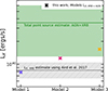 |
Fig. 2. Comparison of the mean point source (AGN and XRB) luminosities from our three forward models (crosses, based on the different halo distributions shown in Fig. 1) with the empirically allowed range of XRB and total point source luminosities, as shown by the hatched gray region and the shaded green region, respectively. We estimate the contribution due to XRB emission using the Aird et al. (2017) model. For estimating the AGN luminosity budget, LX, AGN, we used the Aird et al. (2013) model for the incidence rate distribution as a function of the |

By changing the underlying halo mass distributions for the fixed stellar mass bins, we are effectively altering the mean halo mass of our mock galaxy catalog. We note that for model 3, the resulting mean halo mass lies within the range predicted by various observational and empirical works that constrain the stellar-to-halo-mass relation (SHMR) at low redshift. For the mean stellar mass of our three mock samples (M⋆ = 5.5 × 10¹⁰ M⊙), studies typically find Mhalo ∼ 5 × 10¹¹ M⊙ (Taylor et al. 2020) to 1 − 3 × 10¹² M⊙ (Leauthaud et al. 2012; Coupon et al. 2015; Girelli et al. 2020; Behroozi et al. 2019). Importantly, different simulations predict different SHMRs (see e.g., Wright et al. 2024), and this variation can introduce systematic biases when comparing predicted CGM emission at fixed stellar mass. If the simulated halo mass distribution does not accurately reflect that of the observational sample, the predicted X-ray signal may be systematically over- or under-estimated. For instance, using a simulation that associates higher halo masses at fixed stellar mass than the true sample would yield artificially elevated CGM emission predictions, potentially leading to an erroneous conclusion about a simulation–observation mismatch. This underscores the motivation for our approach: rather than adopting a single SMHM relation, we forward-modeled the halo mass distribution to make it consistent with the data, using observational constraints (further discussed in Sects. 4.1–4.3). Our framework thus enables posterior constraints on the halo mass distribution associated with the Fullphot dataset, based on the TNG-informed models developed in this work. Given the large scatter in halo mass at fixed stellar mass (e.g., Moster et al. 2020), and the strong dependence of CGM surface brightness profiles on this distribution (see right panel of Fig. 1), a rigorous treatment of halo demographics is essential for robust comparisons between simulations and stacked X-ray observations.
4. Results and discussion
We fit the data from Z24 with our three forward models, which contain the hot gas component and the point source component, as shown in Eqs. (1)–(3). The three models emulate different X-ray surface brightness profiles for different halo mass distributions (Sect. 3.3 and Fig. 1). We implemented the Markov chain Monte Carlo (Hastings 1970, MCMC) method to determine the posterior probability distributions of the two free parameters of our models: 𝒩sat and 𝒩ps. The parameters were obtained using the Affine-Invariant Ensemble Sampler algorithm in emcee (Foreman-Mackey et al. 2013). We assumed a Gaussian likelihood function and uniform priors on 𝒩sat ∈ (0.005, 1000)×1035, and 𝒩ps ∈ (0.5, 550)×1035 erg/s/kpc2. For the three forward models constructed in this work, we show the most likely values of the free parameters in Table 1. We computed the luminosities from the hot gas around centrals, satellites, and point sources within R500c5. Fig. 2 shows the mean point source luminosities we obtain for the three models implemented in this work (purple, pink, and yellow crosses). We compare our results with independent predictions on the expected luminosity from XRBs and AGNs around MW-mass galaxies using current empirical models in the literature. Sects. 4.1 and 4.2 describe how we obtain these estimates shown in Fig. 2 for expected luminosity from XRBs and AGNs around MW-mass galaxies.
4.1. Predicting the X-ray emission from XRBs
The XRB emission, which is the X-ray emission from the binary component of stellar populations in normal galaxies, is divided into high-mass X-ray binaries (HXRBs) and low-mass X-ray binaries (LXRBs); see review by Fabbiano (2006). The average XRB emission from a normal galaxy is characterized by scaling laws, where the former HXRB population scales with the recent star formation rate (SFR) in the galaxy (Grimm et al. 2003; Shtykovskiy & Gilfanov 2005; Mineo et al. 2012). In contrast, LXRB emission spans longer timescales, tracing the stellar mass of the galaxy (Gilfanov 2004; Boroson et al. 2011; Zhang et al. 2012; Lehmer et al. 2019). The total XRB emission from extragalactic objects is distributed on the scale of the stellar body; however, for an instrument with a 30 arcsec PSF like eROSITA, it is unresolved and appears as a point source. Aird et al. (2017) and Lehmer et al. (2016) provide simple empirical recipes by parameterizing the total X-ray luminosity from XRBs as a function of both the SFR and stellar mass, M⋆, of the galaxy,
 (4)
(4)
where α, β, γ, δ, and θ are fitting constants. Aird et al. (2017) report the following best-fitting values: log α = 28.81 ± 0.08, γ = 3.90 ± 0.36, log β = 39.50 ± 0.06, δ = 0.67 ± 0.31 and θ = 0.86 ± 0.05.
We quantified the contribution of the total LX, XRB in the LS DR9 Fullphot galaxy catalog using the model from Aird et al. (2017). Since we would later use these estimates to inform our forward models for the allowed range of point source luminosities, we adopted a TNG-independent method of predicting LX, XRB unbiasedly (other reasons for not using TNG are also detailed in Sect. 3.1). We used UCHUU, a suite of ultra-large cosmological N-body simulations (Ishiyama et al. 2021), with the galaxy catalog from UNIVERSEMACHINE (Behroozi et al. 2019) to construct a mock for the Fullphot galaxy sample. The SFRs from UNIVERSEMACHINE were calibrated to reproduce observations. We used the half-sky lightcone, constructed in the procedure detailed in Comparat et al. (2020), to build the mock galaxy catalog. The mocks were generated similarly to Z24, ensuring that the galaxy stellar mass function of the LS DR9 Fullphot galaxy catalog was reproduced. Therefore, they could reliably be used for the purpose of this study. We applied Eq. (4) on the mocks to estimate the contribution of XRBs in the galaxy stack, given the stellar masses and SFR of the mock galaxies. With these ingredients, we predict that the contribution from XRBs alone to be  ergs/s, represented by the hatched gray region in Fig. 26.
4.2. Predicting expected LX, AGN for MW-mass galaxies using an empirical model for the low-redshift Universe
X-ray emission from AGNs originates around an accreting supermassive black hole (see Brandt & Alexander 2015 for a review), appearing as a point-like X-ray source with eROSITA. We proceed to use the empirical model from Aird et al. (2013, hereafter A13) to estimate the LX, AGN for a mean stellar mass M⋆ = 1010.7 M⊙. A13 provide a model for the probability of a galaxy hosting an AGN for a given stellar mass, M⋆, and redshift, z as a function of the specific black hole accretion rate, λ [ergs/s/M⊙]; also called the incidence rate distribution, 𝒫(λ | M⋆, z). The specific accretion rate, λ, of an AGN is the rate at which mass is accreting onto the supermassive black hole. Model C from A13 successfully predicts the XLF and its evolution at 0.2 < z < 1.0. The specific accretion rate, λ, is related to the X-ray luminosity,
![Mathematical equation: $$ \begin{aligned} L_{\rm X,\,AGN}^\mathrm{2{-}10\,keV} = \frac{1}{25}{\lambda \times 1.26 \times 10^{38} \times 0.002\,M_\star \,[\mathrm{ergs\,s^{-1}}]}, \end{aligned} $$](/articles/aa/full_html/2025/11/aa54508-25/aa54508-25-eq21.gif) (5)
(5)
where the 0.002 M⋆ factor represents the mass of the black hole, M•, and assumes correlation between M• and the mass of the bulge, Mbulge (Marconi & Hunt 2003). Additionally, we also assume M⋆ ≈ Mbulge (A13). For the mean of our Fullphot, M⋆ = 1010.7 M⊙ and at the median redshift, ⟨z⟩ = 0.14, we obtain the incidence rate distribution, 𝒫(λ | LX, M⋆, z), as a function of  using Eq. (5). To obtain the 0.5 − 2 keV mean observed X-ray luminosity, which is required to compare with the estimate from this work, we further need to convert the incidence rate distribution from
  to
to  .
.
An important factor that comes into play when performing a conversion from 2 − 10 keV (hard X-ray band; HXB) to the 0.5 − 2 keV (soft X-ray band; SXB) luminosity is the intrinsic obscuration of the AGN. Our estimate of LX, AGN represents the contribution from the obscured AGNs and the observed unobscured Type 1 AGNs, the dominating component at the luminosity range under concern (see e.g., Hasinger 2008). We used the Comparat et al. (2019) empirical obscuration model to obtain the observed HXB-to-SXB luminosity conversion; they self-consistently build an obscuration model based on observation works (Ricci et al. 2017; Buchner & Bauer 2017; Ueda et al. 2014; Aird et al. 2015; Buchner et al. 2015). The Comparat et al. (2019) model is implemented on the UCHUU simulations (introduced in Sect. 4.1), and we obtain the HXB to SXB conversion as a function of  . Finally, we obtain the desired A13-based 𝒫(λ | LX, M⋆, z) distribution as a function of the
  . The expectation value is the obtained as follows:
  .
.
An additional consideration is that the optical sample used for X-ray stacking in Z24 excludes objects classified as point sources in optical. This effectively excludes the optically bright quasars, where the point-like emission strongly dominates over the host galaxy contribution. An unsolved and open question is how such optical selection criteria for AGNs modify the X-ray luminosity distribution in X-rays, and addressing this is beyond the scope of this work. Nonetheless, we proceeded to compute a conservative X-ray luminosity threshold to account for this exclusion of optical quasars as follows. We converted the optical r-band luminosity distribution of the Fullphot galaxy sample to the 2 − 10 keV luminosity distribution using a bolometric correction factor of 2.5 (Collin et al. 2002; Duras et al. 2020; Buchner et al. 2024). We used 10× the mean of the HXB luminosity distribution as the threshold above which the object is classified as a bright point source in the optical LS DR9 catalog. This conservative limit excludes objects with  ergs/s. We adopted this cut in the 𝒫(λ | LX, M⋆, z) distribution as a function of the
  from A13. After applying the obscuration model from Comparat et al. (2019), we obtained
  ergs/s. The sum of LX, AGN computed here and LX, XRB computed in the previous Sect. 4.1 is represented with the shaded green region in Fig. 2.
The large error bars on our estimate of LX, AGN using the methodology described here are due to the uncertainties in the empirical obscuration model and the uncertainties in the incidence rate distribution, which is poorly constrained for the low-redshift Universe. The estimates here can be further improved with future works that strengthen the connection between the low-luminosity X-ray AGN population and the host galaxy properties, proper knowledge mapping AGN selection functions from optical to X-ray luminosities, and better constrained obscuration models.
4.3. Using Model 3 to interpret the Fullphot data
In the light of the empirical estimates we obtain from Sects. 4.1 and 4.2, we compare the prediction for point source luminosities from our three forward models (based on the different halo distribution shown in Fig. 1) with the empirically allowed range of point source luminosities as shown in Fig. 2. This comparison favors model three, which has a mean M200m = 3.5 × 10¹² M⊙, implying that the hot CGM component allows for a point source component with a luminosity that agrees with empirical estimates from the low-redshift Universe. We focus our results on model three for all the following discussions of the hot CGM. The results of fitting model 3 to the X-ray surface brightness profile obtained by stacking on the Fullphot galaxies are shown in Fig. 3, with the posterior distribution of the best-fit parameters shown in Fig. 4.
 |
Fig. 3. Decomposition of the X-ray stack of the galaxies in the photometric sample, Fullphot, into contributions from hot gas events (centrals and satellites hosted by more massive host halos) and point sources (AGNs and XRBs). The orange data points from Z24 are described with the model from this work (shown by the solid black line). The dash-dotted orange line at 292 kpc corresponds to the virial radius of the observational sample. The model is composed of the following: the hot CGM from central galaxies (yellow), the events around satellites probing the hot gas of their more massive host halos (green), and X-ray events from unresolved and resolved point-like sources comprising AGNs and XRBs (gray). The bottom panel shows the percentage deviation of the best-fit forward model from the data. The dash-dotted lines show the 15% level. |
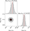 |
Fig. 4. Posterior probability distributions of the renormalization factor of the SX, sat profile: 𝒩sat, and the normalization of the point source component: 𝒩ps, which are obtained by fitting the forward-model 3 from this work to the Fullphot data points from Z24 shown in Fig. 3. The vertical red lines in the diagonal plots correspond to the most likely value; the respective values are mentioned in the titles (refer to Table 1). The dashed black lines are the 68% confidence interval of the marginalized distribution of the free parameters. The contour plot marks the most likely values with the red cross, and the contours correspond to the 68%, 95%, and 99.7% confidence intervals. |
4.4. X-ray emission from the hot CGM
The contribution of the hot CGM component from central galaxies is shown with the yellow line in Fig. 3 for the forward-model 3. By integrating the area under the mean X-ray surface brightness profile from the central galaxy hot CGM component within R500c, we obtain an X-ray luminosity,  ergs/s. We also show the residual plot of the percentage deviation of the data from our model, where the discrepancies are within 15%.
We show the fractional contribution of the various emission components in our forward model 3 to the mean X-ray surface brightness profile upon stacking galaxies in Fig. 5. We note that at mean redshifts of 0.14 and the underlying halo mass distribution for model 3, the hot CGM is unresolved with an eROSITA-like PSF. Thus, at ≲40 kpc, the hot CGM from central galaxies and the X-ray point sources emission from XRBs and AGNs each account for up to 40 − 50% of the total X-ray emission budget, respectively.
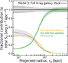 |
Fig. 5. Fractional contribution of centrals, satellites, and point sources to the total X-ray surface brightness profile of the hot CGM. The yellow line shows the contribution from central galaxies, the green line shows the events around satellites probing the hot gas of their more massive host halos, and the dashed gray line shows the X-ray events from unresolved and resolved point-like sources comprising AGNs and XRBs. The errors on the profiles were obtained from the posterior distributions of the MCMC fitting analysis. |
We compare our results with the other hot CGM measurements presented in Z24, based on a different optical galaxy catalog, namely from the SDSS spectroscopic survey. Given the spectroscopic optical information, the galaxy sample is classified into centrals and satellites (Tinker 2021), which makes it possible to empirically model the hot CGM profile from other contaminating effects (point sources and satellites). They selected 30 825 central galaxies with spectroscopic redshifts < 0.2 and MW-like stellar masses of 10.5 < log(M⋆/M⊙) < 11. In Z24, this SDSS-based spectroscopic sample is called the CEN sample. The resulting profile, as shown by the data points in Fig. 6, is compared with the hot CGM component (model 3) we obtain in this work (solid yellow line). Our TNG-based forward model of the hot CGM prediction is in excellent agreement with the hot CGM measurement from Z24 at ≳60 kpc. At the inner radii (≲60 kpc), our TNG-based model 3 overpredicts the X-ray emission. We note that the halo mass distributions of the two samples have similar mean values, where the mean M200m = 3.5 × 10¹² M⊙ for our forward model 3 and the mean  . However, the median
  , highlighting the spread in the halo mass distribution. This result further emphasizes the importance of the underlying halo mass distribution and the impact of the halo mass scatter introduced in stellar-mass selections when comparing hot CGM profiles across different observations and simulation-based models. For reference, we also show the forward models 1 and 2, which we exclude because their hot CGM component does not allow for a permissible contribution of point source luminosity in the X-ray galaxy stack (see Sect. 4.3). In addition to this shortcoming, we find that models 1 and 2 are discrepant with the CEN sample measurement of the hot CGM, further favoring model 3.
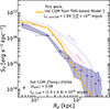 |
Fig. 6. Comparison of the hot gas CGM profile from our TNG-based model 3 (solid yellow line) in this work with the hot CGM measurement from Z24 based on X-ray stacking at the optical positions of galaxies from the SDSS spectroscopic galaxy catalog (CEN sample). The CEN sample has a mean redshift ⟨zspec⟩ = 0.08, which is lower than that for the Fullphot galaxy sample, ⟨zphot⟩ = 0.14, modeled in this work. Therefore, our models (solid yellow, dashed pink, and solid purple) are convolved with the eROSITA PSF representing z = 0.08 to enable comparison with the CEN sample profile from Z24. Our Fullphot-based model 3 convolved with the ⟨zphot⟩ = 0.14 PSF in shown by the dotted yellow line. For reference, we also show the other two models, 1 and 2, with different underlying halo distributions (see text in Sect. 3.3), which we excluded in this work (see Fig. 2) as the hot CGM component did not allow for a point source component with a luminosity consistent with empirical estimates from the low-redshift Universe. The model 3 from this work is in good agreement with the CEN sample hot CGM profile from Z24. |
4.5. X-ray emission from satellite’s host halos
At larger radii (≳40 kpc), the contribution from the emission around satellites dominates the total X-ray signal, thereby explaining the flattening observed in the measurements, as also found by Comparat et al. (2025). This emission originates from the massive host halos in which the satellite galaxies reside; we find the mean host halo mass of these satellites to be M200m ∼ 1014 M⊙. We emphasize that this component is not intended to probe the intrinsic CGM of the satellites themselves, but instead captures the background X-ray emission associated with their host halos. Since the Fullphot galaxy catalog includes both central and satellite galaxies without classification, any observational stacking analysis based on such samples unavoidably includes this contribution. We quantify the X-ray luminosity from satellite host halos as  erg/s, obtained by integrating the area under the predicted surface brightness profile SX, sat. Interestingly, Zhang et al. (2018) also find an inflection point at ∼50 kpc due to satellite’s host halos in the stacked Hα + N[II] radial emission profile (see Fig. 8 therein), where they trace the cool component of the CGM. The findings from Zhang et al. (2018) on the cool CGM is complementary to our results presented here on forward-modeling the hot CGM probed by X-ray stacking.
Upon fitting our forward model to the Fullphot stack, we introduced a renormalization parameter, 𝒩sat, which rescales the SX, sat contribution to match the observations. This scaling was necessary due to the known overprediction of hot gas fractions in TNG300 for halos above 1013.5 M⊙ (Popesso et al. 2024a), leading to an overly bright SX, sat component (see Sect. 3.2). Importantly, the shape of this satellite-related emission component is independent of the satellite fraction, as demonstrated in Fig. 9 in Shreeram et al. (2025). From our fitting analysis for model 3, we find that the TNG-based fiducial SX, sat normalization of the hot CGM must be rescaled by 0.15 to provide an observationally consistent contribution for the Fullphot galaxy catalog based X-ray stack. We highlight that this renormalization does not affect the hot CGM contribution from centrals, which remains unchanged. Therefore, 𝒩sat effectively provides a quantitative correction factor, illustrating how the overabundance of hot gas in massive halos biases the observable MW-mass stacked X-ray profiles. We conclude that the inclusion and forward-modeling of the satellite’s host halo component is required to physically interpret the Fullphot data.
5. Summary
In this work, we have forward-modeled the measurements of the X-ray surface brightness profiles obtained by stacking at the optical galaxy positions of the LS DR9 photometric (Fullphot) galaxy catalog, reported by Z24. We retrieved the contribution of the hot CGM from central galaxies from that of point sources and satellite galaxies. Our hot CGM forward model is based on TNG300 hydrodynamical simulations. The main results from this work are summarized as follows:
-
We tested the impact of the underlying halo mass distribution on the TNG-based prediction for corresponding X-ray surface brightness profiles. We did so by generating multiple mock galaxy catalogs using LC-TNG300, matched in stellar mass and redshift to the Fullphot galaxy catalog; however, with different underlying halo mass distributions (Sect. 3.3; Fig. 1). Namely, the three models obtained by varying the halo mass distribution are as follows: model 1 leaves the LC-TNG300 halo mass distribution unchanged, whereas models 2 and 3 change the underlying halo distribution by excluding the 10% and 30% most massive halos from the original LC-TNG300 halo mass distribution, respectively. We show that the shape and normalization of the hot CGM X-ray surface brightness profiles are impacted by varying the halo mass distributions, whereby discarding the most massive halos from the underlying halo distribution results in steeper profiles with lower normalization. More precisely, we find that a factor ∼2× increase in the mean value of the underlying halo mass distribution results in an ∼4× increase in the X-ray luminosity from the hot CGM.
-
We fit the stacked X-ray radial surface brightness profile by eROSITA around MW-mass galaxies from Zhang et al. (2024a) with our forward models. Our model contains two emitting components (Eqs. 1–3): hot gas (around central galaxies and around satellite galaxies hosted by more massive halos) and X-ray point sources (XRBs and AGNs). For three forward models, we computed the X-ray luminosity from point sources, LX, PS, and CGM (see results in Table 1). Using the empirical estimates for the expected luminosity from XRBs (Sect. 4.1) and AGNs (Sect. 4.2) for MW-mass galaxies, we put constraints on the permissible values of the LX, PS contribution to the X-ray stack (see Fig. 1). This analysis favors model three, which has a mean M200m = 3.5 × 10¹² M⊙, implying that the hot CGM component allows for a point source component with a mean AGN luminosity that agrees with empirical estimates from the low-redshift Universe. We focus our results on model three for all the following discussions of the hot CGM.
-
By integrating the area under the mean X-ray surface brightness profile from the central galaxy hot CGM component within R500c, we obtain an X-ray luminosity of
 ergs/s. We also show the residual plot of the percentage deviation of the data from our model, where the discrepancies within the 50 − 105 kpc range are within 15% (Fig. 3). We find that at ≲40 kpc, the hot CGM from central galaxies and the X-ray point sources emission from XRBs and AGNs each account for 40 − 50% of the total X-ray emission budget, respectively (Fig. 5). At larger radii > 40 kpc, the contribution from the emission around satellites dominates the total X-ray emission, thereby explaining the overall flattening in the measurements.
 -
We compared our results with the other hot CGM measurements presented in Z24, based on a different optical galaxy catalog, namely from the SDSS spectroscopic survey (see comparison in Fig. 6). Our TNG-based forward model of the hot CGM prediction broadly agrees with the hot CGM measurement from Z24. The LX, CGM measured between the two works is consistent. We note that the halo mass distributions of the two samples are similar mean values, where the mean M200m = 3.5 × 10¹² M⊙ for our forward model 3 and the mean
 . This result further emphasizes the importance of the underlying halo mass distribution when comparing hot CGM profiles across different observations and simulation-based models.
This work provides a novel technique to constrain the mean AGN X-ray luminosity of a galaxy sample jointly with the radial hot CGM gas distribution within the halo using the X-ray hot CGM (stacking) measurements as a new benchmark. Alongside the progress in our understanding of how various stellar and AGN feedback prescriptions impact the hot CGM’s properties (Lau et al. 2025; Medlock et al. 2025), here we emphasize another vital ingredient when comparing simulations with X-ray observations: the sensitivity of the X-ray CGM properties to the underlying halo mass distribution, stellar mass, and redshift. One of the outstanding challenges in the current paradigm of galaxy formation and evolution models implemented in hydrodynamical simulations is jointly constraining the microscopic scales (e.g., subgrid model physics) and their impact on the diffuse gas within the halo (Crain & van de Voort 2023). Future work implementing the data-comparison strategy developed here on other state-of-the-art simulations, such as EAGLE (Crain et al. 2015; Schaye et al. 2015), FLAMINGO (Schaye et al. 2023), Magneticum (Dolag et al. 2005; Beck et al. 2016), and SIMBA (Davé et al. 2019), will provide observationally motivated ranges on the allowed X-ray AGN luminosity for the MW-mass scales. Comparing the AGN X-ray luminosity predictions retrieved from the methodology developed here (informed by hot CGM X-ray observations) with those predicted by the simulation itself will provide a new ground for recalibrating and improving the current landscape of sub-grid AGN modes (see e.g., Alexander & Hickox 2012 for a review). Additionally, future X-ray missions on the observation side, such as Athena (Nandra et al. 2013), AXIS (Mushotzky et al. 2019), and HUBS (Cui et al. 2020), will push our current detection limits to resolve the hot CGM at higher redshifts in X-rays. This would further our understanding of how observations compare to the spatially resolved hot gas distribution at MW-mass scales in simulations.
The code to generate lightcones from TNG is publicly available at https://github.com/SoumyaShreeram/LightGen/
This paper defines the stellar mass used from TNG300 as the mass within twice the stellar half-mass radius.
R500c is the radius at which the density of the halo is 500× the critical density of the Universe.
We note that the X-ray scaling relation from Lehmer et al. (2019) predicts  ergs/s for the Fullphot galaxy catalog. Nevertheless, the predictions from using the Aird et al. (2017) and Lehmer et al. (2019) scaling relations are consistent with each other, and we have verified that adopting the Lehmer relation would not change our results.
Acknowledgments
SS would like to thank Fulvio Ferlito and Matteo Guardiani for all the useful scientific discussions. G.P. acknowledges financial support from the European Research Council (ERC) under the European Union’s Horizon 2020 research and innovation program “Hot Milk” (grant agreement No. 865637) and support from Bando per il Finanziamento della Ricerca Fondamentale 2022 dell’Istituto Nazionale di Astrofisica (INAF): GO Large program and from the Framework per l’Attrazione e il Rafforzamento delle Eccellenze (FARE) per la ricerca in Italia (R20L5S39T9). Computations were performed on the HPC system Raven at the Max Planck Computing and Data Facility. We acknowledge the project support by the Max Planck Computing and DataFacility.
References
- Abazajian, K. N., Adelman-McCarthy, J. K., Agüeros, M. A., et al. 2009, ApJS, 182, 543 [Google Scholar]
- Aird, J., Coil, A. L., Moustakas, J., et al. 2013, ApJ, 775, 41 [NASA ADS] [CrossRef] [Google Scholar]
- Aird, J., Coil, A. L., Georgakakis, A., et al. 2015, MNRAS, 451, 1892 [Google Scholar]
- Aird, J., Coil, A. L., & Georgakakis, A. 2017, MNRAS, 465, 3390 [NASA ADS] [CrossRef] [Google Scholar]
- Alexander, D. M., & Hickox, R. C. 2012, New Astron. Rev., 56, 93 [Google Scholar]
- Anders, E., & Grevesse, N. 1989, Geochim. Cosmochim. Acta, 53, 197 [Google Scholar]
- Anderson, M. E., Gaspari, M., White, S. D., Wang, W., & Dai, X. 2015, MNRAS, 449, 3806 [NASA ADS] [CrossRef] [Google Scholar]
- Anderson, M. E., Churazov, E., & Bregman, J. N. 2016, MNRAS, 455, 227 [NASA ADS] [CrossRef] [Google Scholar]
- Beck, A. M., Murante, G., Arth, A., et al. 2016, MNRAS, 455, 2110 [Google Scholar]
- Behroozi, P., Wechsler, R. H., Hearin, A. P., & Conroy, C. 2019, MNRAS, 488, 3143 [NASA ADS] [CrossRef] [Google Scholar]
- Bertone, S., Schaye, J., Dalla Vecchia, C., et al. 2010, MNRAS, 407, 544 [NASA ADS] [CrossRef] [Google Scholar]
- Bhattacharyya, J., Das, S., Gupta, A., Mathur, S., & Krongold, Y. 2023, ApJ, 952, 41 [NASA ADS] [CrossRef] [Google Scholar]
- Biffi, V., Dolag, K., & Böhringer, H. 2013, MNRAS, 428, 1395 [Google Scholar]
- Biffi, V., Dolag, K., & Merloni, A. 2018a, MNRAS, 481, 2213 [Google Scholar]
- Biffi, V., Planelles, S., Borgani, S., et al. 2018b, MNRAS, 476, 2689 [Google Scholar]
- Bogdán, Á., Forman, W. R., Kraft, R. P., & Jones, C. 2013a, ApJ, 772, 98 [CrossRef] [Google Scholar]
- Bogdán, Á., Forman, W. R., Vogelsberger, M., et al. 2013b, ApJ, 772, 97 [CrossRef] [Google Scholar]
- Bogdán, Á., Bourdin, H., Forman, W. R., et al. 2017, ApJ, 850, 98 [CrossRef] [Google Scholar]
- Bogdán, Á., Khabibullin, I., Kovács, O. E., et al. 2023, ApJ, 953, 42 [CrossRef] [Google Scholar]
- Boroson, B., Kim, D.-W., & Fabbiano, G. 2011, ApJ, 729, 12 [NASA ADS] [CrossRef] [Google Scholar]
- Brandt, W., & Alexander, D. 2015, ARA&A, 23, 1 [Google Scholar]
- Buchner, J., & Bauer, F. E. 2017, MNRAS, 465, 4348 [Google Scholar]
- Buchner, J., Georgakakis, A., Nandra, K., et al. 2015, ApJ, 802, 89 [Google Scholar]
- Buchner, J., Starck, H., Salvato, M., et al. 2024, A&A, 692, A161 [NASA ADS] [CrossRef] [EDP Sciences] [Google Scholar]
- Carlson, J., & White, M. 2010, ApJS, 190, 311 [NASA ADS] [CrossRef] [Google Scholar]
- Chadayammuri, U., Bogdán, Á., Oppenheimer, B. D., et al. 2022, ApJ, 936, L15 [NASA ADS] [CrossRef] [Google Scholar]
- Collin, S., Boisson, C., Mouchet, M., et al. 2002, A&A, 388, 771 [NASA ADS] [CrossRef] [EDP Sciences] [Google Scholar]
- Comparat, J., Merloni, A., Salvato, M., et al. 2019, MNRAS, 487, 2005 [Google Scholar]
- Comparat, J., Eckert, D., Finoguenov, A., et al. 2020, Open J. Astrophys., 3, 13 [Google Scholar]
- Comparat, J., Truong, N., Merloni, A., et al. 2022, A&A, 666, A156 [NASA ADS] [CrossRef] [EDP Sciences] [Google Scholar]
- Comparat, J., Merloni, A., Ponti, G., et al. 2025, A&A, 697, A173 [NASA ADS] [CrossRef] [EDP Sciences] [Google Scholar]
- Coupon, J., Arnouts, S., van Waerbeke, L., et al. 2015, MNRAS, 449, 1352 [NASA ADS] [CrossRef] [Google Scholar]
- Crain, R. A., & van de Voort, F. 2023, ARA&A, 61, 473 [NASA ADS] [CrossRef] [Google Scholar]
- Crain, R. A., Schaye, J., Bower, R. G., et al. 2015, MNRAS, 450, 1937 [NASA ADS] [CrossRef] [Google Scholar]
- Cui, W., Chen, L.-B., Gao, B., et al. 2020, J. Low Temp. Phys., 199, 502 [NASA ADS] [CrossRef] [Google Scholar]
- Das, S., Mathur, S., Gupta, A., et al. 2019, ApJ, 885, 108 [NASA ADS] [CrossRef] [Google Scholar]
- Davé, R., Anglés-Alcázar, D., Narayanan, D., et al. 2019, MNRAS, 486, 2827 [Google Scholar]
- Dey, A., Schlegel, D. J., Lang, D., et al. 2019, ApJ, 157, 168 [CrossRef] [Google Scholar]
- Dolag, K., Grasso, D., Springel, V., & Tkachev, I. 2005, JCAP, 2005, 009 [Google Scholar]
- Dolag, K., Borgani, S., Murante, G., & Springel, V. 2009, MNRAS, 399, 497 [Google Scholar]
- Donahue, M., & Voit, G. M. 2022, Phys. Rep., 973, 1 [NASA ADS] [CrossRef] [Google Scholar]
- Donnari, M., Pillepich, A., Nelson, D., et al. 2019, MNRAS, 485, 4817 [Google Scholar]
- Donnari, M., Pillepich, A., Nelson, D., et al. 2021, MNRAS, 506, 4760 [NASA ADS] [CrossRef] [Google Scholar]
- Duras, F., Bongiorno, A., Ricci, F., et al. 2020, A&A, 636, A73 [NASA ADS] [CrossRef] [EDP Sciences] [Google Scholar]
- Fabbiano, G. 2006, ARA&A, 44, 323 [NASA ADS] [CrossRef] [Google Scholar]
- Faucher-Giguère, C.-A., & Oh, S. P. 2023, ARA&A, 61, 131 [CrossRef] [Google Scholar]
- Foreman-Mackey, D., Hogg, D. W., Lang, D., & Goodman, J. 2013, PASP, 125, 306 [Google Scholar]
- Foster, A., Ji, L., Smith, R., & Brickhouse, N. 2012, ApJ, 756, 128 [Google Scholar]
- Galeazzi, M., Gupta, A., Covey, K., & Ursino, E. 2007, ApJ, 658, 1081 [NASA ADS] [CrossRef] [Google Scholar]
- Gilfanov, M. 2004, MNRAS, 349, 146 [NASA ADS] [CrossRef] [Google Scholar]
- Girelli, G., Pozzetti, L., Bolzonella, M., et al. 2020, A&A, 634, A135 [NASA ADS] [CrossRef] [EDP Sciences] [Google Scholar]
- Grimm, H. J., Gilfanov, M., & Sunyaev, R. 2003, MNRAS, 339, 793 [Google Scholar]
- Habouzit, M., Genel, S., Somerville, R. S., et al. 2019, MNRAS, 484, 4413 [CrossRef] [Google Scholar]
- Hasinger, G. 2008, A&A, 490, 905 [NASA ADS] [CrossRef] [EDP Sciences] [Google Scholar]
- Hastings, W. K. 1970, Biometrika, 57, 97 [Google Scholar]
- Ishiyama, T., Prada, F., Klypin, A. A., et al. 2021, MNRAS, 506, 4210 [NASA ADS] [CrossRef] [Google Scholar]
- Koutroumpa, D., Acero, F., Lallement, R., Ballet, J., & Kharchenko, V. 2007, A&A, 475, 901 [NASA ADS] [CrossRef] [EDP Sciences] [Google Scholar]
- Lau, E. T., Nagai, D., Bogdán, Á., et al. 2025, ApJ, 984, 190 [Google Scholar]
- Leauthaud, A., Tinker, J., Bundy, K., et al. 2012, ApJ, 744, 159 [Google Scholar]
- Lehmer, B., Basu-Zych, A., Mineo, S., et al. 2016, ApJ, 825, 7 [Google Scholar]
- Lehmer, B. D., Eufrasio, R. T., Tzanavaris, P., et al. 2019, ApJS, 243, 3 [NASA ADS] [CrossRef] [Google Scholar]
- Li, J.-T., Bregman, J. N., Wang, Q. D., et al. 2017, ApJS, 233, 20 [NASA ADS] [CrossRef] [Google Scholar]
- Locatelli, N., Ponti, G., Zheng, X., et al. 2024, A&A, 681, A78 [NASA ADS] [CrossRef] [EDP Sciences] [Google Scholar]
- Marconi, A., & Hunt, L. K. 2003, ApJ, 589, L21 [Google Scholar]
- Marinacci, F., Vogelsberger, M., Pakmor, R., et al. 2018, MNRAS, 480, 5113 [NASA ADS] [Google Scholar]
- Mathur, S., Das, S., Gupta, A., & Krongold, Y. 2023, MNRAS, 525, L11 [Google Scholar]
- Medlock, I., Neufeld, C., Nagai, D., et al. 2025, ApJ, 980, 61 [Google Scholar]
- Merloni, A., Lamer, G., Liu, T., et al. 2024, A&A, 682, A34 [NASA ADS] [CrossRef] [EDP Sciences] [Google Scholar]
- Mineo, S., Gilfanov, M., & Sunyaev, R. 2012, MNRAS, 419, 2095 [Google Scholar]
- Moster, B. P., Naab, T., & White, S. D. M. 2020, MNRAS, 499, 4748 [Google Scholar]
- Mushotzky, R., Aird, J., Barger, A. J., et al. 2019, BAAS, 51, 107 [Google Scholar]
- Naiman, J. P., Pillepich, A., Springel, V., et al. 2018, MNRAS, 477, 1206 [Google Scholar]
- Nandra, K., Barret, D., Barcons, X., et al. 2013, ArXiv e-prints [arXiv:1306.2307] [Google Scholar]
- Nelson, D., Pillepich, A., Genel, S., et al. 2015, Astron. Comput., 13, 12 [Google Scholar]
- Nelson, D., Springel, V., Pillepich, A., et al. 2019, Comput. Astrophys. Cosmol., 6, 2 [Google Scholar]
- Oppenheimer, B. D., Bogdán, Á., Crain, R. A., et al. 2020, ApJ, 893, L24 [NASA ADS] [CrossRef] [Google Scholar]
- Pillepich, A., Nelson, D., Hernquist, L., et al. 2018, MNRAS, 475, 648 [Google Scholar]
- Planck Collaboration XIII. 2016, A&A, 594, A13 [NASA ADS] [CrossRef] [EDP Sciences] [Google Scholar]
- Ponti, G., Zheng, X., Locatelli, N., et al. 2023, A&A, 674, A195 [NASA ADS] [CrossRef] [EDP Sciences] [Google Scholar]
- Popesso, P., Biviano, A., Marini, I., et al. 2024a, A&A, submitted [arXiv:2411.16555] [Google Scholar]
- Popesso, P., Marini, I., Dolag, K., et al. 2024b, A&A, submitted [arXiv:2411.17120] [Google Scholar]
- Ricci, C., Trakhtenbrot, B., Koss, M. J., et al. 2017, Nature, 549, 488 [NASA ADS] [CrossRef] [Google Scholar]
- Rohr, E., Pillepich, A., Nelson, D., Ayromlou, M., & Zinger, E. 2024, A&A, 686, A86 [NASA ADS] [CrossRef] [EDP Sciences] [Google Scholar]
- Rosas-Guevara, Y., Bower, R. G., Schaye, J., et al. 2016, MNRAS, 462, 190 [CrossRef] [Google Scholar]
- Schaye, J., Crain, R. A., Bower, R. G., et al. 2015, MNRAS, 446, 521 [Google Scholar]
- Schaye, J., Kugel, R., Schaller, M., et al. 2023, MNRAS, 526, 4978 [NASA ADS] [CrossRef] [Google Scholar]
- Shreeram, S., Comparat, J., Merloni, A., et al. 2025, A&A, 697, A22 [NASA ADS] [CrossRef] [EDP Sciences] [Google Scholar]
- Shtykovskiy, P., & Gilfanov, M. 2005, MNRAS, 362, 879 [NASA ADS] [CrossRef] [Google Scholar]
- Sijacki, D., Vogelsberger, M., Genel, S., et al. 2015, MNRAS, 452, 575 [NASA ADS] [CrossRef] [Google Scholar]
- Smith, R. K., Brickhouse, N. S., Liedahl, D. A., & Raymond, J. C. 2001, ApJ, 556, L91 [Google Scholar]
- Springel, V., White, S. D., Tormen, G., & Kauffmann, G. 2001, MNRAS, 328, 726 [NASA ADS] [CrossRef] [Google Scholar]
- Springel, V., Pakmor, R., Pillepich, A., et al. 2018, MNRAS, 475, 676 [Google Scholar]
- Strauss, M. A., Weinberg, D. H., Lupton, R. H., et al. 2002, ApJ, 124, 1810 [Google Scholar]
- Taylor, E. N., Cluver, M. E., Duffy, A., et al. 2020, MNRAS, 499, 2896 [Google Scholar]
- Tinker, J. L. 2021, ApJ, 923, 154 [NASA ADS] [CrossRef] [Google Scholar]
- Tumlinson, J., Peeples, M. S., & Werk, J. K. 2017, ARA&A, 55, 389 [Google Scholar]
- Ueda, Y., Akiyama, M., Hasinger, G., Miyaji, T., & Watson, M. G. 2014, ApJ, 786, 104 [Google Scholar]
- van de Voort, F. 2013, MNRAS, 430, 2688 [NASA ADS] [CrossRef] [Google Scholar]
- Vladutescu-Zopp, S., Biffi, V., & Dolag, K. 2023, A&A, 669, A34 [NASA ADS] [CrossRef] [EDP Sciences] [Google Scholar]
- Volonteri, M., Dubois, Y., Pichon, C., & Devriendt, J. 2016, MNRAS, 460, 2979 [Google Scholar]
- Wechsler, R. H., & Tinker, J. L. 2018, ARA&A, 56, 435 [NASA ADS] [CrossRef] [Google Scholar]
- Weng, S., Péroux, C., Ramesh, R., et al. 2024, MNRAS, 527, 3494 [Google Scholar]
- Wijers, N. A., Schaye, J., & Oppenheimer, B. D. 2020, MNRAS, 498, 574 [NASA ADS] [CrossRef] [Google Scholar]
- Wright, R. J., Somerville, R. S., Lagos, C. D. P., et al. 2024, MNRAS, 532, 3417 [NASA ADS] [CrossRef] [Google Scholar]
- Zhang, Z., Gilfanov, M., & Bogdán, Á. 2012, A&A, 546, A36 [NASA ADS] [CrossRef] [EDP Sciences] [Google Scholar]
- Zhang, H., Zaritsky, D., & Behroozi, P. 2018, ApJ, 861, 34 [NASA ADS] [CrossRef] [Google Scholar]
- Zhang, Z., Wang, H., Luo, W., et al. 2022, A&A, 663, A85 [NASA ADS] [CrossRef] [EDP Sciences] [Google Scholar]
- Zhang, Y., Comparat, J., Ponti, G., et al. 2024a, A&A, 690, A267 [NASA ADS] [CrossRef] [EDP Sciences] [Google Scholar]
- Zhang, Y., Comparat, J., Ponti, G., et al. 2024b, A&A, 690, A268 [NASA ADS] [CrossRef] [EDP Sciences] [Google Scholar]
- Zheng, X., Ponti, G., Locatelli, N., et al. 2024, A&A, 689, A328 [NASA ADS] [CrossRef] [EDP Sciences] [Google Scholar]
- Zou, H., Gao, J., Zhou, X., & Kong, X. 2019, ApJS, 242, 8 [Google Scholar]
- Zou, H., Sui, J., Xue, S., et al. 2022, RAA, 22, 065001 [NASA ADS] [Google Scholar]
- ZuHone, J. A., & Hallman, E. J. 2016, Astrophysics Source Code Library [record ascl:1608.002] [Google Scholar]
All Tables
All Figures
|
Fig. 1. Forward models constructed in this work for the hot CGM from central galaxies by varying the underlying halo mass distribution. Left panel: Purple halo mass distribution (Model 1) obtained from the mock central galaxy catalog – constructed with the TNG300 lightcone (LC-TNG300) from Shreeram et al. (2025) – for the X-ray stack from Z24 that uses optically detected galaxies with photometric redshifts (Fullphot) from LS DR9 (Dey et al. 2019). Note that the mock galaxy catalog is generated by matching LC-TNG300 to Fullphot in stellar mass and redshift (see details in Sect. 3.3); the median stellar mass and redshift of the Fullphot (and our mock catalogs) are 5.5 × 10¹⁰ M⊙ and 0.14, respectively. The underlying halo mass distribution of the Fullphot optical dataset is unknown. The pink distribution (Model 2; with mean M200m = 5.4 × 10¹² M⊙) discards the top 10% most massive halos before the generation of the mock galaxy catalog. The yellow distribution (Model 3; with mean M200m = 3.5 × 10¹² M⊙) discards the top 30% most massive halos before the generation of the mock galaxy catalog. Right panel: Corresponding X-ray surface brightness profiles in the 0.5 − 2 kev energy band (for details on their generation see Sect. 3.2) for the three mock galaxy catalogs with different halo mass distributions, which are shown in the left panel. The profiles are convolved with the eROSITA PSF, and they represent the Fullphot dataset in the stellar mass and redshift plane. Nevertheless, due to the impact of the underlying halo mass distribution, the shape and normalization of the hot CGM profiles are impacted, where discarding the most massive halos from the underlying halo distribution results in steeper profiles with lower normalizations. |
| In the text | |
|
Fig. 2. Comparison of the mean point source (AGN and XRB) luminosities from our three forward models (crosses, based on the different halo distributions shown in Fig. 1) with the empirically allowed range of XRB and total point source luminosities, as shown by the hatched gray region and the shaded green region, respectively. We estimate the contribution due to XRB emission using the Aird et al. (2017) model. For estimating the AGN luminosity budget, LX, AGN, we used the Aird et al. (2013) model for the incidence rate distribution as a function of the |
| In the text | |
|
Fig. 3. Decomposition of the X-ray stack of the galaxies in the photometric sample, Fullphot, into contributions from hot gas events (centrals and satellites hosted by more massive host halos) and point sources (AGNs and XRBs). The orange data points from Z24 are described with the model from this work (shown by the solid black line). The dash-dotted orange line at 292 kpc corresponds to the virial radius of the observational sample. The model is composed of the following: the hot CGM from central galaxies (yellow), the events around satellites probing the hot gas of their more massive host halos (green), and X-ray events from unresolved and resolved point-like sources comprising AGNs and XRBs (gray). The bottom panel shows the percentage deviation of the best-fit forward model from the data. The dash-dotted lines show the 15% level. |
| In the text | |
|
Fig. 4. Posterior probability distributions of the renormalization factor of the SX, sat profile: 𝒩sat, and the normalization of the point source component: 𝒩ps, which are obtained by fitting the forward-model 3 from this work to the Fullphot data points from Z24 shown in Fig. 3. The vertical red lines in the diagonal plots correspond to the most likely value; the respective values are mentioned in the titles (refer to Table 1). The dashed black lines are the 68% confidence interval of the marginalized distribution of the free parameters. The contour plot marks the most likely values with the red cross, and the contours correspond to the 68%, 95%, and 99.7% confidence intervals. |
| In the text | |
|
Fig. 5. Fractional contribution of centrals, satellites, and point sources to the total X-ray surface brightness profile of the hot CGM. The yellow line shows the contribution from central galaxies, the green line shows the events around satellites probing the hot gas of their more massive host halos, and the dashed gray line shows the X-ray events from unresolved and resolved point-like sources comprising AGNs and XRBs. The errors on the profiles were obtained from the posterior distributions of the MCMC fitting analysis. |
| In the text | |
|
Fig. 6. Comparison of the hot gas CGM profile from our TNG-based model 3 (solid yellow line) in this work with the hot CGM measurement from Z24 based on X-ray stacking at the optical positions of galaxies from the SDSS spectroscopic galaxy catalog (CEN sample). The CEN sample has a mean redshift ⟨zspec⟩ = 0.08, which is lower than that for the Fullphot galaxy sample, ⟨zphot⟩ = 0.14, modeled in this work. Therefore, our models (solid yellow, dashed pink, and solid purple) are convolved with the eROSITA PSF representing z = 0.08 to enable comparison with the CEN sample profile from Z24. Our Fullphot-based model 3 convolved with the ⟨zphot⟩ = 0.14 PSF in shown by the dotted yellow line. For reference, we also show the other two models, 1 and 2, with different underlying halo distributions (see text in Sect. 3.3), which we excluded in this work (see Fig. 2) as the hot CGM component did not allow for a point source component with a luminosity consistent with empirical estimates from the low-redshift Universe. The model 3 from this work is in good agreement with the CEN sample hot CGM profile from Z24. |
| In the text | |
Current usage metrics show cumulative count of Article Views (full-text article views including HTML views, PDF and ePub downloads, according to the available data) and Abstracts Views on Vision4Press platform.
Data correspond to usage on the plateform after 2015. The current usage metrics is available 48-96 hours after online publication and is updated daily on week days.
Initial download of the metrics may take a while.