| Issue |
A&A
Volume 703, November 2025
|
|
|---|---|---|
| Article Number | A284 | |
| Number of page(s) | 8 | |
| Section | Stellar atmospheres | |
| DOI | https://doi.org/10.1051/0004-6361/202554940 | |
| Published online | 24 November 2025 | |
An on-the-fly line-driven wind iterative mass-loss estimator (LIME) for hot, massive stars of arbitrary chemical compositions
Instituut voor Sterrenkunde, KU Leuven,
Celestijnenlaan 200D,
3001
Leuven,
Belgium
★ Corresponding author: This email address is being protected from spambots. You need JavaScript enabled to view it.
Received:
1
April
2025
Accepted:
2
October
2025
Abstract
Context. Mass-loss rates, Ṁ, from hot, massive stars are important for a range of astrophysical applications.
Aims. We present LIME, a fast, efficient, and easy-to-use real-time mass-loss calculator for line-driven winds from hot, massive stars with given stellar parameters and arbitrary chemical compositions. The tool is publicly available online.
Methods. We compute the line force on-the-fly from excitation and ionization balance calculations using a large atomic data base containing more than four million spectral lines. We then derive mass-loss rates from line-driven wind theory, including effects of a finite stellar disk and gas sound speed.
Results. For a given set of stellar parameters and chemical composition, we obtain predictions for Ṁ and for the three line-force parameters, Q̄, Q0, and α, at the wind critical point. A comparison of our predicted Ṁ with a large sample of recent, state-of-the-art, homogeneously derived empirical mass-loss rates obtained from the XSHOOTU collaboration project demonstrates that the simple calculator presented here performs on average as well as, or even better than, other available mass-loss recipes based on fits to restricted model grids computed from more sophisticated but less flexible methods.
Conclusions. In addition to its speed and simplicity, a strength of our mass-loss calculator is that it avoids uncertainties related to applying fit formulae to underlying model grids calculated for more restricted parameter ranges. In particular, individual chemical abundances can be easily modified, and their effects on predicted mass-loss rates can be readily explored. This enables direct applications also to stars that are significantly chemically modified at the surface.
Key words: radiation: dynamics / methods: analytical / methods: numerical / stars: massive / stars: mass-loss / stars: winds, outflows
© The Authors 2025
 Open Access article, published by EDP Sciences, under the terms of the Creative Commons Attribution License (https://creativecommons.org/licenses/by/4.0), which permits unrestricted use, distribution, and reproduction in any medium, provided the original work is properly cited.
This article is published in open access under the Subscribe to Open model. This email address is being protected from spambots. You need JavaScript enabled to view it. to support open access publication.
1 Introduction
For hot, massive stars, absorption and scattering in spectral lines transfer significant momentum from the star’s intense radiation field to the plasma, providing a force that can overcome gravity and drive a strong, fast wind outflow. Line-driven wind theory based on this mechanism was established in the seminal paper by Castor et al. (1975) (hereafter CAK). Earlier attempts (e.g., Lucy & Solomon 1970) focused on obtaining the line force from a small number of select lines, whereas CAK used results obtained for carbon to parametrize the cumulative line acceleration stemming from numerous lines. While various extensions and reformulations of this elegant model have substantially improved its quantitative applicability as well as our physical understanding (e.g., Abbott 1982; Friend & Castor 1983; Owocki & Rybicki 1984; Pauldrach et al. 1986; Owocki et al. 1988; Kudritzki et al. 1989; Gayley 1995; Cranmer & Owocki 1995; Puls et al. 2000; Kudritzki & Puls 2000; Kudritzki 2002; Curé 2004; Lattimer & Cranmer 2021; Poniatowski et al. 2022; Key et al. 2025), many key elements of line-driven wind theory were undoubtedly already established by CAK.
Much effort has been devoted to obtaining quantitative predictions for mass-loss rates, Ṁ, suitable for direct comparisons with observations and for applications such as stellar evolution and feedback. Typically, models in this category have used detailed radiative transfer techniques applied directly to large discrete line lists; examples include models based on the comoving frame (CMF; Pauldrach et al. 1986; Sander et al. 2017; Krtička & Kubát 2017; Sundqvist et al. 2019) as well as Monte Carlo (Vink et al. 2000; Lucy 2010) radiative transfer. Since these calculations are very time-consuming, a commonly used approach has been to compute relatively small grids of models and then design “mass-loss recipes” by fitting grid results to some assumed functional behavior of Ṁ with stellar parameters (e.g., Vink et al. 2001; Sander & Vink 2020; Björklund et al. 2021, 2023; Krticka et al. 2024). Although these approaches have been very useful, the resulting recipes are very inflexible because the underlying model-grid calculations are computationally intensive. Consequently, many applications in practice rely on (sometimes questionable) extrapolations to domains outside the actual model grids. Moreover, differences between actual model-grid results and the applied fit formulas introduce significant scatter and additional uncertainty. Another important aspect of the effort here is that, in general, it has not yet been possible to directly examine the effects of varying individual chemical abundances on line-driven mass-loss predictions, although a few targeted attempts have been made (e.g., Vink & de Koter 2005; Krticka et al. 2019). In practice, this means that applications often rely only on simple scaling relations with overall metallicity (e.g., Meynet et al. 2006).
Building on line-driven wind theory, we present a fast and reliable method for directly computing line-driven mass-loss
rates from stars with given stellar parameters and arbitrary abundance patterns. We tested this method by comparison with state-of-the-art observational results from the large XSHOOT ULLYSES project (Vink et al. 2023), showing that our method performs better than several more elaborate but less flexible mass-loss recipes that are currently available. Motivated by these results, we provide a new, user-friendly online mass-loss calculator LIME, which accepts arbitrary stellar parameters and chemical compositions (within our recommended limits, see Sect. 4). On-the-fly calculations typically take only a few seconds, and users can also submit larger batch jobs. Our method is therefore well suited for direct applications to observed stars with specific parameters, as well as for broader applications such as stellar evolution and feedback.
2 Method and applicability
To compute mass-loss rates we applied CAK theory as formulated by Gayley (1995), modified for a high-opacity cut-off in line strength (Owocki et al. 1988), including the finite-disk angle effect (Pauldrach et al. 1986) according to Kudritzki et al. (1989), and a finite sound speed correction following Owocki & ud-Doula (2004). The analytic mass-loss rate as derived from the modified CAK critical point analysis is therefore
 (1)
(1)
as given, for example, by Gayley (1995) (their Eq. (43)), applying a finite-disk correction factor from Kudritzki et al. (1989, Eq. (32)) and a sound-speed correction as outlined in Appendix A of Owocki & ud-Doula (2004). Here, L is the stellar luminosity, c the speed of light, Γe ≡ ge∣g = Lκe∣(4πcGM) the classical Eddington ratio for electron scattering opacity κe and stellar mass M, a is the isothermal gas sound speed, and  the escape speed from the stellar surface, reduced by the contribution from Γe. The line-force parameters are Q̅, Q0, and α. For a given set of stellar parameters, the present problem is thus reduced to finding appropriate values for these and for κe at the wind critical point.
The line acceleration,  , is computed from the sum
 (2)
(2)
for a line list consisting of N lines, each indexed by i, so that M(t) defines the line-force multiplier with respect to the electron-scattering acceleration, ge. Here qi = kL,i∣(v0ρκe) is the normalized line strength for the frequency-integrated line extinction coefficient kL [cm−1Hz] and line-center frequency ν0, wν,i is the frequency-dependent flux weighting with fluxes approximated as Planckian distributions Poniatowski et al. (2022) (see also Puls et al. 2000), and qit = τi is the line optical depth τi Sobolev (1960). Importantly, since t = κecρ/|dv/dr| is independent of the line index i, it can be treated as an independent variable of the problem (Castor et al. 1975). For further discussions and full derivations of these quantities, we refer to Poniatowski et al. (2022), in particular Sects. 2.1-2.2. As in Poniatowski et al. (2022), we computed this sum for a range of t by solving the excitation and ionization balance for a given mass density, ρ, and temperature, T, using the Munich atomic line database (Pauldrach et al. 2001; Puls et al. 2000, 2005)1 and following the Saha-Boltzmann procedure outlined in Poniatowski et al. (2022) (see also Lattimer & Cranmer 2021). We then fit the result to
 (3)
(3)
This functional form follows from the line-distribution function of Gayley (1995) (see Sect. 2.3 in Poniatowski et al. 2022). For a given (ρ, T) pair, the fit provides values of Q0 and α, while Q can be computed directly from the sum in Eq. (2); representative examples are shown in Fig. 1. The quantity Q̅ ≡ Σi wν,iqi sets the saturation for the force multiplier in the limit that all lines are optically thin. The parameter Q0 is related to the position where the optically thick lines begin to appear, and α determines the slope of M(t) in the region where these effects are visi-ble2. The physical meaning of these parameters is discussed in Gayley (1995); Puls et al. (2000); Poniatowski et al. (2022)3. We evaluate the line-force parameters at the wind critical point and inserted into the mass-loss rate formula above. Ionization and recombination keep the wind approximately at the photospheric temperature (Puls et al. 2000) so we set T = Teff for our calculations (see also Lattimer & Cranmer 2021). The critical point density, ρc, is initially unknown. For a critical point velocity, vc, and radius, rc, we compute ρc = Ṁ/(4πvcrc2). We apply the finite-disk effect (Pauldrach et al. 1986), which places the wind critical point very close to the stellar surface, R*, so that rc = R* is generally a good approximation. For the critical velocity vc we apply the modified CAK “cooking recipe” of Kudritzki et al. (1989) (see their Eqs. (55, 55a)).
For each set of stellar parameters and chemical composition, we first guess values for the line-force parameters, applying Eq. (1) and computing an initial estimate of ρc. Using this estimate, we solve for the sum in Eq. (2) for a range of t, fit Eq. (3) to the results and obtain updated values for the line-force parameters. We then use the updated parameters to compute a new mass-loss rate and repeated the procedure until ρc (and hence Ṁ) converged. This procedure yields a simple, robust, fast, and efficient scheme that typically achieves good precision after very few iteration steps (often only about four; see Fig. 2). The results are predictions for Ṁ and values of Q̄, Q0, and α at the wind critical point for each set of stellar input parameters. A typical example of the iteration is shown in Fig. 2. An interactive version of the procedure is available at LIME4.
Occasionally, different parts of the M(t) curve for a given (ρ, T) pair have different slopes. This typically occurs at relatively low temperatures, as shown in Fig. 1 (orange circles). Fig. 3 demonstrates that this behavior relates to the contributions of different driving ions to the total line force. In the example shown, the iron line contribution (green curve) displays a shallower slope than the carbon, nitrogen, and oxygen (CNO) lines and a significantly lower saturation limit, Q̄. While iron contributes significantly to the total line force at higher t values, CNO dominates M(t) at lower t, which is then also reflected in the slope of the cumulative curve. This slope difference between light (CNO) and heavy (iron) elements was also found by Puls et al. (2000). To ensure that we covered the “correct” part of the M(t) curve, we estimated tcri = κeρcrc/|dv/drcr| using the analytically predicted velocity gradient for the critical point in the CAK radial stream limit. When fitting for Q0 and α, we then ensured that the fitting range included both tcri and the saturation limit. The latter is particularly important because saturation occurs at different t values in different parts of the parameter space (for example, depending on metallicity, Z).
A reasonable lower limit for line-driven winds is Γe (1 + Q̄) > 1, since below this the radiation force is never able to overcome gravity5. As such, we imposed Γe(1 + Q̄) = 1 as a lower limit for our models, but note that a somewhat stricter limit of the present theory could be M(tcri) < Q̄. If this criterion is not met, the line-force multiplier does not depend on the velocity gradient, rendering the CAK-like critical point analysis leading to Eq. (1) questionable. Although not relevant for the observational comparisons presented in Sect. 3, these lower limits can be important for cases with low Γe and in the low-metallicity regime (see also Kudritzki 2002), owing to the principal dependence Q̄ ~ Z. Finally, we note that we did not consider possible decoupling of metal ions from the bulk hydrogen and helium plasma, which may complicate the situation for very low-density winds (see Owocki & Puls 2002 for suitable estimates of where this effect might become relevant).
The present version of LIME evaluates the line force parameters only at the estimated wind critical point, which determines the mass-loss rate within the formalism. As such, the effects of relative differences in line-driving efficiency between the inner and outer wind regions are neglected (see also Sect. 4). However, we can still use the line-force parameters calculated by LIME to obtain also an approximate value for the terminal wind speed v∞. For this, we adopted the fitting-formulas of Kudritzki & Puls (2000, Eqs. (15) and (17), assuming δ = 0). As noted above, because our method does not take into account differences in line-driving efficiency between the wind critical point and the outer wind, terminal wind speed estimates are generally expected to be less precise than our corresponding Ṁ calculations (see, e.g., Puls et al. 2000; Björklund et al. 2021 for discussions of how outer-wind effects may influence v∞). When comparing our theoretical 3∞ estimates with values from the empirical studies described below, we find reasonably good agreement for early supergiants, whereas theoretical values for dwarfs are sometimes higher than empirically inferred v∞- a general result that has been noted several times before in the line-driven wind literature (e.g.,Kudritzki & Puls 2000; Björklund et al. 2021).
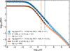 |
Fig. 1 Line-force multiplier, M(t), as a function of the Sobolev optical-depth-like parameter, t. The blue diamonds and orange circles show the line-force multiplier calculated for the characteristic density, temperature, and metallicity listed in the labels. Black lines indicate the best fits with the corresponding line-force parameters. Relative metal abundances are scaled to the solar metallicity of Asplund et al. (2009). |
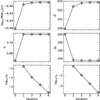 |
Fig. 2 Quantities Ṁ (top left), Q̄ (top right), α (middle left), and Q0 (middle right) as a function of iteration number until convergence (after 3 iterations). The bottom panels show relative differences in Ṁ (left) and critical point density ρ (right) between successive iterations. |
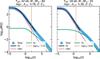 |
Fig. 3 Line-force multiplier, M(t), as a function of t for stars with Teff and critical point density (log ρcrit [g cm−3]) of 42 000 [K] and -12.79 (left) and 18 000 [K] and -14.52 (right). The line-force parameters Q, Q0, and α at the critical point are 1043, 620, 0.73 (left) and 866, 834, 0.87 (right). Blue circles represent M(t) calculated from the entire line list, with the black line indicating the fit. Green and pink lines show M(t) calculated using only Fe lines and CNO lines, respectively. The vertical dashed orange line marks tcri (see text). |
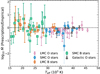 |
Fig. 4 Logarithm of the ratio between mass-loss rates derived using our method and rates obtained empirically from observational data as described in the text. The colors and markers correspond to the different samples marked on the labels. The dashed line illustrates the position where rates would be equal. |
3 Comparison with observations and other theoretical mass-loss rates
Fig. 4 compares our predicted mass-loss rates with those derived from observations of 86 OB stars in the Galaxy, the large Magellanic cloud (LMC), and small Magellanic cloud (SMC). These empirical rates were derived homogeneously by fitting optical and ultraviolet observations of a multitude of strategic spectral lines to synthetic spectra computed with the model atmosphere and wind code FASTWIND (Puls et al. 2005; Sundqvist & Puls 2018). This modeling accounts for wind clumping with arbitrary optical thickness, a non-void interclump medium, and porosity effects in velocity space. Observational data were taken from the ULYSSES and XSHOOTU projects (Vink et al. 2023) for the LMC and SMC, and from Hawcroft et al. (2021) for the Galaxy. For each star, we used a genetic algorithm approach to find the global best fit to the data (Hawcroft et al. 2021; Brands et al. 2022). These state-of-the-art empirical results are described in detail by Hawcroft et al. (2021); Verhamme et al. (2024); Backs et al. (2024); Brands et al. (2025), and Verhamme et al. (in prep.).
Fig. 4 shows overall good agreement between our predicted rates and those empirically inferred from observations. The error bars indicate 1σ statistical uncertainties in the empirical Ṁ. Although the comparison exhibits significant scatter, there appears to be no significant systematics present. Comparing our predictions with alternative mass-loss rate recipes from Vink et al. (2001); Björklund et al. (2023) and Krticka et al. (2024), shown in Fig. 5 reveals that the simple method presented here performs equally well or better. For example, the systematics seen in the comparisons with Vink et al. (2001), which predicts significantly higher rates at lower temperatures, and with Björklund et al. (2023), which systematically yields lower rates, were not present in our results. The prescription of Krticka et al. (2024) also shows no clear systematics, but we note that this recipe is based on a complex fitting function formula applied to an underlying model grid. This makes its application outside the limited parameter domain (logl0 L/L⊙ = 5.28-5.88 and Z/Z⊙ = 0.2-1.0) difficult and not recommended (see discussions in Krticka et al. 2024 and Verhamme et al. 2024). Sample means and standard deviations of all four comparisons yield the ratios log10 , and -0.30 ± 0.34 for the present method and those of Vink et al. (2001), Björklund et al. (2023), and Krticka et al. (2024), respectively; these sample means and standard deviations are also plotted in the lower panel of Fig. 5. It remains unclear whether the remaining small offset and scatter in the comparisons between our method and the empirical data are dominated by uncertainties in the line-driven wind theory presented here or in the methods used to infer Ṁ from observational data (see also the discussions in Björklund et al. 2021; Verhamme et al. 2024).
We also provide the line-force parameters (α, Q̄), and Q0) for the stars in our comparison sample (see Fig. 6). As expected, the Q̄ values are on average higher for LMC stars than for SMC stars because of the higher metallicity of the LMC; however, significant star-to-star scatter is present. We also note an interesting feature of large α values at lower temperatures. The explanation for this is the same as that discussed in Fig. 3: whereas the slope of the M(t) curve is shallower in the iron-dominated high-t regions, tcri for our sample stars typically falls within the steeper region influenced by lighter CNO ions, resulting in higher characteristic α values. This trend contrasts previous discussions in the line-driven wind literature regarding which ions primarily set Ṁ. Specifically, while such discussions (e.g., Puls et al. 2000) primarily focused on the role of CNO in outer wind driving at Galactic metallicities, we find that the steeper slopes of these lighter ions are often already reflected in the accumulative line force at M(tcri).
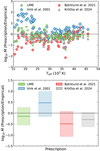 |
Fig. 5 Top panel: same as Fig. 4, but also comparing the observations with theoretical rates computed by different methods, as indicated in the labels. For clarity, error margins for empirical rates are omitted. Bottom panel: sample averages and one standard deviation for the four methods. The dashed black line indicates where rates are equal. |
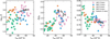 |
Fig. 6 Line-force parameters Q̄ (left), Q̄/Q0 (middle), and α (right) at the wind critical point for the stellar sample described in Sect. 3. Colors and markers correspond to the different stellar types indicated in the labels. |
4 Discussion and conclusion
The observational comparisons presented above demonstrate that our simple mass-loss calculator performs equally well or better than alternative recipes based on more elaborate line-driven wind models. This may partly arise because those recipes are fit formulas, typically assuming a power-law scaling of Ṁ with stellar parameters, based on underlying grid calculations for a restricted number of models. This introduces scatter and uncertainties when applied to actual stars (see Sect. 3). In contrast, our method computes all quantities on-the-fly for any given set of input stellar parameters, thereby avoiding such intrinsic uncertainties. Moreover, with our approach, we can directly tune individual abundances, whereas Vink et al. (2001); Björklund et al. (2023); Krticka et al. (2024) provide only general scalings with overall metallicity Z. As an example of this advantage, although the general scaling Q̄ ~ Z holds (Gayley 1995), stars with significant surface chemical modifications do not always follow this. Secondary effects from corresponding changes in Q0 and α can also affect the final Ṁ scalings with metallicity differently, depending on the stellar parameter range (see also Puls et al. 2000). We anticipate this to be especially relevant for future applications to chemically modified stars in the early Universe (e.g., Meynet et al. 2006) and to stars stripped by binary interactions (e.g., Götberg et al. 2023).
Overall, LIME yields better agreement with empirical studies than the theoretical rates we previously computed from the same atomic database. These rates were calculated using more sophisticated CMF radiative-transfer methods coupled with a full solution to the stationary equation of motion (Sundqvist et al. 2019, with corresponding grid calculations by Björklund et al. 2021, 2023). In these CMF-based models, a local reduction in radiative acceleration around the gas sonic point, generally related to a source function dip (see Owocki & Puls 1999), effectively limits the mass flux that can be driven. This is in contrast to models using Sobolev (1960) line transfer and results in overall lower predicted mass-loss rates, particularly for dwarf stars. Furthermore, inclusion of ad hoc so-called “microturbulence” in the broadening of line profiles significantly impacts the predicted line force in such non-Sobolev models (see Lucy 2010; Björklund et al. 2021; González-Torà et al. 2025). Recent time-dependent multidimensional simulations of O stars reveal strong turbulence in the sonic regions (Debnath et al. 2024). However, our results suggest that including this turbulence using the current standard “microturbulence” framework in stationary CMF-based models may not be justified, at least not when computing the line acceleration. In Appendix A, we further compare force multipliers computed with the Saha Boltzmann method used here to those obtained with the approximate NLTE method of Puls et al. (2000). For a few select temperatures at a prototypical critical point density, we derived line-force parameters using both methods and find generally small differences. The main reason is that the mass-loss rate is determined very close to the stellar surface. At these radii, the densities are still relatively high and the effects of NLTE modest6. In the outer wind, NLTE effects are typically much larger due to the very diluted stellar radiation field. This underlies why LIME provides better results for Ṁ than for v∞ (see the end of Sect. 2). Specifically, our method uses insights from line-driven wind theory to avoid explicit numerical solutions of the equation of motion, thereby obtaining mass-loss rates in a simplified way. It therefore computes the line force at a single (critical) point in the wind. This method can then provide on-the-fly quantitative predictions for mass-loss rates, since computing the sum in Eq. (2) is the only time-expensive step in the algorithm. In reality, however, density and temperature vary throughout the wind, so that the excitation and ionization balance, and thus the line-force parameters Q̄, Q0, and α, also vary (see Poniatowski et al. 2022; Moens et al. 2022a; Debnath et al. 2024 for examples of these variations within this formalism). This also applies to NLTE corrections, which generally increase with wind radius. These effects influence the analytic estimates of the wind-critical position and velocity applied here (see also Kudritzki et al. 1989; Puls et al. 2000). However, the comparisons in Sect. 3 and Appendix A suggest that they do not, in general, significantly affect the calculations of global Ṁ from line-driven winds.
Due to limitations in our atomic database, we currently do not recommend applying the recipe outside the range 18 kK ≲ Teff ≲ 60 kK. We are currently working on an extension to lower and higher temperatures and will report on this in the near future (Debnath et al., in prep.). Such extensions are important, for example, for evolved hot stars whose surface layers have been stripped by binary interactions (Götberg et al. 2023).
In addition to these temperature restrictions, a few further limitations of our method are worth noting. (i) Although the calculator can technically be applied up to the limit Γe → 1, the theory is based on line-driving from the stellar surface, which means subsurface physical effects may complicate applications for stars residing very close to the classical Eddington limit, at least at (near) Galactic metallicities and above (see also Bestenlehner 2020). Recent multidimensional simulations of evolved stars with Z = Z⊙ show that above a certain Γe threshold, opacities from ionization of iron-group elements around T ~ 150 kK (Rogers & Iglesias 1992) provide enough radiation force to launch a strong wind outflow from beneath the stellar surface, leading to enhanced mass-loss rates if the wind is also sustained to higher radii (Moens et al. 2022b). Similar results have also been found for recent 1D, stationary models (Sander et al. 2020). However, this effect is strongly metallicity dependent, so that hot stars with significantly lower abundances of iron-group elements can reside much closer to the Eddington limit with undergoing subsurface wind launch. (ii) We neglect the effects of rotation; for fast-rotating stars, corrections may be required (see Sect. 2.2.1 of Puls et al. 2008). (iii) We also neglect the influence of strong magnetic fields, which, at least for a small subset of massive stars, can induce magnetospheres that prevent large portions of the initiated wind from escaping the star (see Ud-Doula et al. 2008, their Eq. (23), for a suitable scaling relation).
Acknowledgements
The authors gratefully acknowledge support from the European Research Council (ERC) Horizon Europe under grant agreement number 101044048, from the Belgian Research Foundation Flanders (FWO) Odysseus program under grant number G0H9218N, from FWO grant G077822N, and from KU Leuven C1 grant BRAVE C16/23/009. The authors would also like to thank previous members of the KUL-EQUATION group for their earlier contributions, and the referee for their useful comments on the manuscript. Finally, JS extends his personal thanks to (the both retiring) Jo Puls and Stan Owocki, for teaching him lots of stuff about line-driven winds over the years. The following packages were used to analyze the data: NumPy (Harris et al. 2020), SciPy (Virtanen et al. 2020), matplotlib (Hunter 2007).
References
- Abbott, D. C. 1982, ApJ, 259, 282 [Google Scholar]
- Abbott, D. C., & Lucy, L. B. 1985, ApJ, 288, 679 [NASA ADS] [CrossRef] [Google Scholar]
- Asplund, M., Grevesse, N., Sauval, A. J., & Scott, P. 2009, ARA&A, 47, 481 [NASA ADS] [CrossRef] [Google Scholar]
- Backs, F., Brands, S. A., de Koter, A., et al. 2024, A&A, 692, A88 [NASA ADS] [CrossRef] [EDP Sciences] [Google Scholar]
- Bestenlehner, J. M. 2020, MNRAS, 493, 3938 [Google Scholar]
- Björklund, R., Sundqvist, J. O., Puls, J., & Najarro, F. 2021, A&A, 648, A36 [EDP Sciences] [Google Scholar]
- Björklund, R., Sundqvist, J. O., Singh, S. M., Puls, J., & Najarro, F. 2023, A&A, 676, A109 [NASA ADS] [CrossRef] [EDP Sciences] [Google Scholar]
- Brands, S. A., de Koter, A., Bestenlehner, J. M., et al. 2022, A&A, 663, A36 [Google Scholar]
- Brands, S. A., Backs, F., de Koter, A., et al. 2025, A&A, 697, A54 [NASA ADS] [CrossRef] [EDP Sciences] [Google Scholar]
- Castor, J. I., Abbott, D. C., & Klein, R. I. 1975, ApJ, 195, 157 [Google Scholar]
- Cranmer, S. R., & Owocki, S. P. 1995, ApJ, 440, 308 [NASA ADS] [CrossRef] [Google Scholar]
- Curé, M. 2004, ApJ, 614, 929 [CrossRef] [Google Scholar]
- Debnath, D., Sundqvist, J. O., Moens, N., et al. 2024, A&A, 684, A177 [NASA ADS] [CrossRef] [EDP Sciences] [Google Scholar]
- Friend, D. B., & Castor, J. I. 1983, ApJ, 272, 259 [NASA ADS] [CrossRef] [Google Scholar]
- Gayley, K. G. 1995, ApJ, 454, 410 [Google Scholar]
- González-Torà, G., Sander, A. A. C., Moens, N., et al. 2025, A&A, 699, A244 [NASA ADS] [CrossRef] [EDP Sciences] [Google Scholar]
- Götberg, Y., Drout, M. R., Ji, A. P., et al. 2023, ApJ, 959, 125 [CrossRef] [Google Scholar]
- Harris, C. R., Millman, K. J., van der Walt, S. J., et al. 2020, Nature, 585, 357 [NASA ADS] [CrossRef] [Google Scholar]
- Hawcroft, C., Sana, H., Mahy, L., et al. 2021, A&A, 655, A67 [NASA ADS] [CrossRef] [EDP Sciences] [Google Scholar]
- Hunter, J. D. 2007, Comput. Sci. Eng., 9, 90 [NASA ADS] [CrossRef] [Google Scholar]
- Key, J., Proga, D., Dannen, R., Vivier, S., & Waters, T. 2025, APJ, 987, 144 [Google Scholar]
- Krticka, J., & Kubát, J. 2017, A&A, 606, A31 [NASA ADS] [CrossRef] [EDP Sciences] [Google Scholar]
- Krticka, J., Janik, J., Krticková, I., et al. 2019, A&A, 631, A75 [NASA ADS] [CrossRef] [EDP Sciences] [Google Scholar]
- Krticka, J., Kubát, J., & Krticková, I. 2024, A&A, 681, A29 [NASA ADS] [CrossRef] [EDP Sciences] [Google Scholar]
- Kudritzki, R. P. 2002, ApJ, 577, 389 [NASA ADS] [CrossRef] [Google Scholar]
- Kudritzki, R.-P., & Puls, J. 2000, ARA&A, 38, 613 [Google Scholar]
- Kudritzki, R. P., Pauldrach, A., Puls, J., & Abbott, D. C. 1989, A&A, 219, 205 [NASA ADS] [Google Scholar]
- Lattimer, A. S., & Cranmer, S. R. 2021, ApJ, 910, 48 [CrossRef] [Google Scholar]
- Lucy, L. B. 2010, A&A, 524, A41 [NASA ADS] [CrossRef] [EDP Sciences] [Google Scholar]
- Lucy, L. B., & Abbott, D. C. 1993, ApJ, 405, 738 [Google Scholar]
- Lucy, L. B., & Solomon, P. M. 1970, ApJ, 159, 879 [Google Scholar]
- Meynet, G., Ekström, S., & Maeder, A. 2006, A&A, 447, 623 [NASA ADS] [CrossRef] [EDP Sciences] [Google Scholar]
- Moens, N., Poniatowski, L. G., Hennicker, L., et al. 2022a, A&A, 665, A42 [NASA ADS] [CrossRef] [EDP Sciences] [Google Scholar]
- Moens, N., Sundqvist, J. O., El Mellah, I., et al. 2022b, A&A, 657, A81 [NASA ADS] [CrossRef] [EDP Sciences] [Google Scholar]
- Owocki, S. P., & Puls, J. 1999, ApJ, 510, 355 [Google Scholar]
- Owocki, S. P., & Puls, J. 2002, ApJ, 568, 965 [NASA ADS] [CrossRef] [Google Scholar]
- Owocki, S. P., & Rybicki, G. B. 1984, ApJ, 284, 337 [Google Scholar]
- Owocki, S. P., & ud-Doula, A. 2004, ApJ, 600, 1004 [NASA ADS] [CrossRef] [Google Scholar]
- Owocki, S. P., Castor, J. I., & Rybicki, G. B. 1988, ApJ, 335, 914 [NASA ADS] [CrossRef] [Google Scholar]
- Pauldrach, A., Puls, J., & Kudritzki, R. P. 1986, A&A, 164, 86 [NASA ADS] [Google Scholar]
- Pauldrach, A. W. A., Hoffmann, T. L., & Lennon, M. 2001, A&A, 375, 161 [NASA ADS] [CrossRef] [EDP Sciences] [Google Scholar]
- Petrenz, P., & Puls, J. 2000, in Astronomical Society of the Pacific Conference Series, 214, IAU Colloq. 175: The Be Phenomenon in Early-Type Stars, eds. M. A. Smith, H. F. Henrichs, & J. Fabregat, 626 [Google Scholar]
- Poniatowski, L. G., Kee, N. D., Sundqvist, J. O., et al. 2022, A&A, 667, A113 [NASA ADS] [CrossRef] [EDP Sciences] [Google Scholar]
- Puls, J., Springmann, U., & Lennon, M. 2000, A&AS, 141, 23 [NASA ADS] [CrossRef] [EDP Sciences] [Google Scholar]
- Puls, J., Urbaneja, M. A., Venero, R., et al. 2005, A&A, 435, 669 [NASA ADS] [CrossRef] [EDP Sciences] [Google Scholar]
- Puls, J., Vink, J. S., & Najarro, F. 2008, A&A Rev., 16, 209 [NASA ADS] [CrossRef] [Google Scholar]
- Rogers, F. J., & Iglesias, C. A. 1992, ApJS, 79, 507 [CrossRef] [Google Scholar]
- Sander, A. A. C., & Vink, J. S. 2020, MNRAS, 499, 873 [Google Scholar]
- Sander, A. A. C., Hamann, W. R., Todt, H., Hainich, R., & Shenar, T. 2017, A&A, 603, A86 [NASA ADS] [CrossRef] [EDP Sciences] [Google Scholar]
- Sander, A. A., Vink, J. S., & Hamann, W.-R. 2020, MNRAS, 491, 4406 [Google Scholar]
- Sobolev, V. V. 1960, Moving Envelopes of Stars (Cambridge: Harvard University Press) [Google Scholar]
- Sundqvist, J. O., & Puls, J. 2018, A&A, 619, A59 [NASA ADS] [CrossRef] [EDP Sciences] [Google Scholar]
- Sundqvist, J. O., Björklund, R., Puls, J., & Najarro, F. 2019, A&A, 632, A126 [NASA ADS] [CrossRef] [EDP Sciences] [Google Scholar]
- Ud-Doula, A., Owocki, S. P., & Townsend, R. H. D. 2008, MNRAS, 385, 97 [NASA ADS] [CrossRef] [Google Scholar]
- Verhamme, O., Sundqvist, J., de Koter, A., et al. 2024, A&A, 692, A91 [NASA ADS] [CrossRef] [EDP Sciences] [Google Scholar]
- Vink, J. S., & de Koter, A. 2005, A&A, 442, 587 [NASA ADS] [CrossRef] [EDP Sciences] [Google Scholar]
- Vink, J. S., de Koter, A., & Lamers, H. J. G. L. M. 2000, A&A, 362, 295 [Google Scholar]
- Vink, J. S., de Koter, A., & Lamers, H. J. G. L. M. 2001, A&A, 369, 574 [NASA ADS] [CrossRef] [EDP Sciences] [Google Scholar]
- Vink, J. S., Mehner, A., Crowther, P. A., et al. 2023, A&A, 675, A154 [NASA ADS] [CrossRef] [EDP Sciences] [Google Scholar]
- Virtanen, P., Gommers, R., Oliphant, T. E., et al. 2020, Nat. Methods, 17, 261 [Google Scholar]
This database consists of >4 million lines covering all elements from hydrogen to zinc (except Li, Be, B, and Sc, which are too rare to affect the accumulative line-opacity) and ionization stages up to VIII. It is the same database as included in the model-atmosphere code FASTWIND (see Puls et al. 2005, their Sect. 3).
In their study, CAK considered only this power-law component.
Because we obtain a new excitation and ionisation balance for each pair of (ρ, T), there is no need to introduce additional parameters, such as Abbott 1982’s δ-parameter (see Poniatowski et al. 2022) when fitting M(t) using Eq. (3).
Gas pressure gradients are typically small in regimes where linedriving is important.
This applies to the evaluation of cumulative line acceleration, but may not hold for detailed diagnostics of specific spectral lines (see Appendix A and Puls et al. 2005).
Appendix A NLTE effects
We here evaluate potential NLTE effects on the line force multipliers computed by LIME. For this purpose we use the method applied in the line-driven wind statistics paper by Puls et al. (2000) for computing the ionisation balance and occupation numbers. This is an approximate NLTE method that modifies the Saha-Boltzmann relations by accounting explicitly for different radiation and gas temperatures, Trad and Tgas, as well as for a modified spherical dilution factor W of the illuminating radiation field (as defined in, e.g., Eq. (10) of Lucy & Abbott 1993). In comparison to the standard dilution factor, note that this modified W contains an optical depth correction such that, by definition, W = 1 at the stellar surface in order to obtain a smooth transition to LTE conditions. This approximate method (or variants of it) has been quite extensively and successfully applied before in a range of line-driven wind studies (for example by Abbott 1982; Abbott & Lucy 1985; Lucy & Abbott 1993; Puls et al. 2000; Petrenz & Puls 2000), and has also been calibrated against full NLTE calculations in Puls et al. (2005). We here follow Puls et al. (2000) in using a frequency-independent radiation temperature and a Planckian radiation field, enabling straightforward and direct comparisons to results in the main paper. As discussed in Puls et al. (2000) (their Sect. 4.2.8), previous tests using more realistic photospheric fluxes generally show small effects, with the possible exception of cooler B-stars (see also Petrenz & Puls 2000). As we currently cut application of LIME at Teff = 18 kK we adhere to Planckian fluxes in this paper, deferring further studies of the influence from different irradiation fluxes to future work (which in any case would involve computations of newer and much larger grids of underlying model atmospheres in order to allow for general applications).
Fig. A.1 shows force multipliers M(t) and fitted line-force parameters Q̄, Q0, and α computed with the new method. For a typical critical point density, results for four different gas temperatures are shown. Tgas = Trad and W = 1 here correspond to the LTE approximation used in LIME, and we have verified that results are indeed identical. We test this against the ratio Tgas/Trad = 0.8, also used by Puls et al. (2000), and for W = 1 as well as a very diluted radiation field W = 1/3 as in table 2 of Puls et al. 2000. From the figure we see that effects upon derived line force parameters are insignificant for all combinations with W = 1 and remain generally small also for W = 1/3 (e.g., changes in α < 0.1 throughout), albeit with some moderately large changes in Q0 present. Most importantly though, corresponding effects upon predicted mass-loss rates remain modest. Note also that application of the low W = 1/3 means that the critical point would be shifted away from the stellar surface, which is not what our method here assumes and generally goes against the trend for line-driven wind models including the finite stellar disk (and even more so for models based on co-moving frame radiative transfer, see below).
The relatively small NLTE effects found here are quite interesting in view of the general consensus that such effects are always very important in hot star atmospheres. But as discussed also in the main paper, this is particularly true further out in the wind where the radiation field is very diluted. On the other hand, near the star where the mass-loss rate is set, gas and radiation temperatures remain relatively similar and the radiation field is only modestly diluted. It is still true that a frequency-dependent radiation temperature and NLTE calculations are critical for certain population numbers (e.g., the HeII ground state, see Puls et al. 2005) and the formation of specific spectral lines, but the results presented here suggest that for the cumulative line acceleration such effects may perhaps play a somewhat smaller role than previously thought, at least near the stellar surface. Since the critical point is even closer to the surface (at the gas sonic point) in non-Sobolev stationary wind models based on co-moving frame line radiative transfer (Sander et al. 2017; Sundqvist et al. 2019), this may at least partly explain why the simple semi-analytic LTE method presented in this paper actually gives results that, in a general sense, agree rather well with these seemingly much more sophisticated simulations. Indeed, this was actually suggested already by the small set of full hydrodynamical LTE O-star line-driven wind simulations by Poniatowski et al. (2022), who found overall good agreement with the mass-loss rates predicted by complete NLTE models (their Fig. 7).
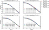 |
Fig. A.1 Force multipliers M(t) computed for the densities and temperatures shown at top of each plot. Each plot shows four different M(t) curves and corresponding fits of Q̄, Q0, and α, computed for the different combinations of dilution factor W, radiation temperature Trad, and gas temperature Tgas, displayed in the colour bar to the right. The temperatures T at the top of each figure refer to Trad. |
All Figures
|
Fig. 1 Line-force multiplier, M(t), as a function of the Sobolev optical-depth-like parameter, t. The blue diamonds and orange circles show the line-force multiplier calculated for the characteristic density, temperature, and metallicity listed in the labels. Black lines indicate the best fits with the corresponding line-force parameters. Relative metal abundances are scaled to the solar metallicity of Asplund et al. (2009). |
| In the text | |
|
Fig. 2 Quantities Ṁ (top left), Q̄ (top right), α (middle left), and Q0 (middle right) as a function of iteration number until convergence (after 3 iterations). The bottom panels show relative differences in Ṁ (left) and critical point density ρ (right) between successive iterations. |
| In the text | |
|
Fig. 3 Line-force multiplier, M(t), as a function of t for stars with Teff and critical point density (log ρcrit [g cm−3]) of 42 000 [K] and -12.79 (left) and 18 000 [K] and -14.52 (right). The line-force parameters Q, Q0, and α at the critical point are 1043, 620, 0.73 (left) and 866, 834, 0.87 (right). Blue circles represent M(t) calculated from the entire line list, with the black line indicating the fit. Green and pink lines show M(t) calculated using only Fe lines and CNO lines, respectively. The vertical dashed orange line marks tcri (see text). |
| In the text | |
|
Fig. 4 Logarithm of the ratio between mass-loss rates derived using our method and rates obtained empirically from observational data as described in the text. The colors and markers correspond to the different samples marked on the labels. The dashed line illustrates the position where rates would be equal. |
| In the text | |
|
Fig. 5 Top panel: same as Fig. 4, but also comparing the observations with theoretical rates computed by different methods, as indicated in the labels. For clarity, error margins for empirical rates are omitted. Bottom panel: sample averages and one standard deviation for the four methods. The dashed black line indicates where rates are equal. |
| In the text | |
|
Fig. 6 Line-force parameters Q̄ (left), Q̄/Q0 (middle), and α (right) at the wind critical point for the stellar sample described in Sect. 3. Colors and markers correspond to the different stellar types indicated in the labels. |
| In the text | |
|
Fig. A.1 Force multipliers M(t) computed for the densities and temperatures shown at top of each plot. Each plot shows four different M(t) curves and corresponding fits of Q̄, Q0, and α, computed for the different combinations of dilution factor W, radiation temperature Trad, and gas temperature Tgas, displayed in the colour bar to the right. The temperatures T at the top of each figure refer to Trad. |
| In the text | |
Current usage metrics show cumulative count of Article Views (full-text article views including HTML views, PDF and ePub downloads, according to the available data) and Abstracts Views on Vision4Press platform.
Data correspond to usage on the plateform after 2015. The current usage metrics is available 48-96 hours after online publication and is updated daily on week days.
Initial download of the metrics may take a while.