| Issue |
A&A
Volume 703, November 2025
|
|
|---|---|---|
| Article Number | A80 | |
| Number of page(s) | 11 | |
| Section | Astrophysical processes | |
| DOI | https://doi.org/10.1051/0004-6361/202555000 | |
| Published online | 06 November 2025 | |
Testing the effect of the progenitor metallicity on the 56Ni mass and constraining the progenitor scenarios in Type Ia supernovae
1
Department of Astronomy, Yonsei University, Seoul 03722, Republic of Korea
2
Center for Galaxy Evolution Research, Yonsei University, Seoul 03722, Republic of Korea
⋆ Corresponding author: This email address is being protected from spambots. You need JavaScript enabled to view it.
Received:
2
April
2025
Accepted:
6
September
2025
Abstract
The analytical model found that the intrinsic variation in the initial metallicity of the Type Ia supernova (SN Ia) progenitor stars (Zprogenitor) translates into a 25% variation in the synthesized 56Ni mass, and therefore, into a difference of ∼0.2 mag in the observed peak luminosity of SNe Ia. Previous observational studies used the currently observed global gas-phase metallicity of host galaxies, instead of Zprogenitor that was used in the model, and the studies showed a higher scatter in the 56Ni mass measurements than the model prediction. We used Zprogenitor of 34 normal SNe Ia and employed recent SN Ia explosion models with various configurations to cover the observed 56Ni mass range. Unlike previous studies, which only used samples in the sub-solar range, our sample covers the Zprogenitor range (1/3 Z⊙ < Zprogenitor < 3 Z⊙), where most of the Zprogenitor effect occurs. Linear regression returns a slope of 0.02 ± 0.03, which trend is opposite to that of the analytical model, but at at low statistical significance level. A comparison of our sample with SN Ia explosion models on the Zprogenitor–56Ni mass diagram allowed us to constrain the progenitor scenarios. We also explored other chemical composition indicators, such as (Fe/H)progenitor and (α/Fe)progenitor. For (Fe/H)progenitor, our sample follows the trend predicted by the analytical models, but at a low significance level (0.4σ). Noticeably, (α/Fe)progenitor shows the opposite trend and a clear gap. When we split the sample at (α/Fe)progenitor = 0.35(α/Fe)⊙, we find a 3σ difference in the weighted means of the 56Ni mass. Lastly, the standardized luminosities of SNe Ia in different Zprogenitor groups differed by 0.14 ± 0.09 (1.6σ) mag. We highlight a holistic approach (from the progenitor star to the explosion with SN Ia and host galaxy observational data) to understanding the underlying physics of SNe Ia for a more accurate and precise cosmology.
Key words: methods: data analysis / stars: abundances / supernovae: general / galaxies: abundances / distance scale
© The Authors 2025
 Open Access article, published by EDP Sciences, under the terms of the Creative Commons Attribution License (https://creativecommons.org/licenses/by/4.0), which permits unrestricted use, distribution, and reproduction in any medium, provided the original work is properly cited.
This article is published in open access under the Subscribe to Open model. This email address is being protected from spambots. You need JavaScript enabled to view it. to support open access publication.
1. Introduction
The peak luminosity of Type Ia supernovae (SNe Ia) is an essential ingredient for their use as distance indicators. The empirical relation between the peak luminosity and its decline rate (Phillips 1993) and also its peak colour (Tripp 1998) reduced the intrinsic variation in the SN Ia peak luminosity in the V band from ∼1 mag to ∼0.1 mag. From this accuracy, SNe Ia provided direct observational evidence of the accelerating expansion of the Universe (Riess et al. 1998; Perlmutter et al. 1999). Recently, combined with other cosmological probes, some challenges in cosmology were reported, such as the Hubble tension (Riess et al. 2022) and a preference for dynamical dark energy (DESI Collaboration 2025). Although SNe Ia play an important role in cosmology, the physical origin of the empirical relation and the peak luminosity variation in SNe Ia remains elusive. Therefore, understanding this would help us to alleviate the challenges we face currently.
The intrinsic variation in the SN Ia peak luminosity is theoretically tightly correlated with the amount of 56Ni that is synthesized during the explosion because the explosion of SNe Ia is powered by the radioactive decay of 56Ni (Truran et al. 1967; Colgate & McKee 1969). This 56Ni amount presumably depends on the properties of the progenitor star (e.g., mass and metallicity) and on the details of the explosion scenarios (near-Chandrasekhar or sub-Chandrasekhar mass (Mch) and deflagration or detonation explosions). In this regard, Timmes et al. (2003, hereafter TBT03) analytically explored how the intrinsic variation in the initial metallicity of the SN Ia progenitor stars (Zprogenitor) translates into a variation in the synthesized 56Ni mass and therefore, into the peak luminosity of an SNe Ia.
TBT03 assumed that nearly all one-dimensional Mch models of SNe Ia produce most of the 56Ni in a burn to nuclear statistical equilibrium between the mass shells of 0.2 and 0.8 M⊙. They found a linear relation between Zprogenitor and the 56Ni mass,
 (1)
(1)
This is because higher-metallicity main-sequence stars are expected to evolve into white dwarfs (WDs) with more neutron-rich elements, producing more stable burning products relative to radioactive 56Ni. TBT03 suggested that the progenitor metallicity accounts for a 25% variation in 56Ni mass that is synthesized in SNe Ia, and thus, to ∼0.2 mag in the observed peak luminosity of SNe Ia in the V band.
After TBT03, several studies were conducted to update this analytical model. Howell et al. (2009, hereafter H09) accounted for the fact that O/Fe can vary as a function of Fe/H, such that [O/Fe] = a + b [Fe/H] taken from Ramírez et al. (2007), while TBT03 assumed that O/Fe is constant relative to Fe/H. Ramírez et al. (2007) fitted this linear relation and provided coefficients of a and b for different populations of stars in the thin disk, the thick disk, and the halo (see their Table 3 for a and b values of each population). H09 considered these different populations of stars when they calculated O/Fe via different a and b values. Then, with [O/Fe] = [O/H] − [Fe/H], they suggested a linear relation between the 56Ni mass synthesized in SNe Ia and O/H and also Fe/H1,
![Mathematical equation: $$ \begin{aligned} \dfrac{M_{56}}{M^{0}_{56}}&= 1 - 0.044 \left[ \frac{\mathrm{(O/H)}}{10^{-3}} \right] \left\{ 1 + 0.122 \left[ \frac{\mathrm{(O/H)}}{10^{-3}} \right] \right. \nonumber \\&\quad \left. + 10^{-(0.19+0.53b+a)/(1+b)} \left[ \frac{(\mathrm {O/H})}{10^{-3}} \right] ^{-b/(1+b)} \right\} ,\end{aligned} $$](/articles/aa/full_html/2025/11/aa55000-25/aa55000-25-eq3.gif) (2)
(2)
![Mathematical equation: $$ \begin{aligned} \dfrac{M_{56}}{M^{0}_{56}}&= 1 - 0.020 \times 10^{a+(1+b)[\mathrm {Fe/H}]} \{1 + 0.056 \times 10^{a+(1+b)[\mathrm {Fe/H}]} \nonumber \\&\quad + 0.64 \times 10^{-a-b[\mathrm {Fe/H}]} \}. \end{aligned} $$](/articles/aa/full_html/2025/11/aa55000-25/aa55000-25-eq4.gif) (3)
(3)
Here,  is the synthesized 56Ni mass at an electron abundance equal to
  , that is, for a pure C–O WD. We note that H09 used the Asplund et al. (2005) abundances for the solar composition.
Another update of TBT03 was made by Bravo et al. (2010, hereafter B10). They suggested a steeper slope of 0.075 (see their Equation (2)) than that of TBT03 based on a series of SNe Ia explosion simulations, considering the Mch deflagration-to-detonation transition models with a central density of a WD (ρc) = 3 × 10⁹ g cm−3 and Zprogenitor = 10−5–0.10 Z⊙. They also explored a non-linear relation considering the deflagration-to-detonation transition density as a function of the local Zprogenitor,
 (4)
(4)
Some studies tested the TBT03 model with observational data, for example, Gallagher et al. (2005), H09, and Neill et al. (2009), Moreno-Raya et al. (2016). These studies used the average metallicity of the SN Ia host galaxies or the regions around the SN Ia explosion site rather than Zprogenitor because Zprogenitor is difficult to determine through observation. Gallagher et al. (2005) used spectroscopic line ratios of 30 host galaxies to determine the metallicity and found that the correlation was at the 70% confidence level. H09 and Neill et al. (2009) tested the model with more samples in intermediate- and low-redshift ranges, respectively. They inferred the metallicity from the stellar mass of the host galaxies using the mass-metallicity relation of Tremonti et al. (2004) and Lee et al. (2006), and they concluded that their data were consistent with the TBT03 prediction updated by H09. Moreno-Raya et al. (2016) observed and estimated the metallicity of the 28 regions in which the SNe Ia exploded. Instead of using 56Ni mass, they used the absolute magnitude of SNe Ia, which is positively correlated with the 56Ni mass. They found a probability of 80% of a correlation between the absolute SN Ia magnitude and the local metallicity, in the sense that the SN Ia luminosities tend to be higher for galaxies with lower metallicities. All previous studies using observational data of host galaxies or regions around SN Ia explosion sites presented the same trend as the TBT03 model, even though the scatter in 56Ni mass measurements is higher than the TBT03 prediction.
More precisely, previous studies used the currently observed global gas-phase metallicity (e.g. 12 + log(O/H)). A recent study by Kim et al. (2024, hereafter K24) showed that there is a difference in metallicity between the SN Ia birth environment and the currently observed status of host galaxies because of the delay time between the birth of the progenitor star and the SN Ia explosion. This means that the currently observed global metallicity used in previous studies is not representative of Zprogenitor (see also a discussion in Section 5 of Howell et al. 2009). In addition, TBT03 defined the metallicity as the CNO + Fe abundances, like the total stellar metallicity. Although the total stellar and gas-phase metallicity are correlated (e.g., Cid Fernandes et al. 2005), they are not identical. Lastly, previous studies did not have enough samples in the higher-metallicity range, where most progenitor metallicity effects occur.
Furthermore, regarding the higher scatter in 56Ni mass measurements than predicted by the TBT03 model, this implies that the analytical model cannot fully account for the observed 56Ni production of SNe Ia. However, recent hydrodynamic simulations of SN Ia explosion models with different explosion mechanisms and progenitor properties, including the Zprogenitor dependence, can produce the observed 56Ni mass range (e.g., Leung & Nomoto 2018, 2020; Gronow et al. 2021). In addition to the 56Ni abundance, these studies provide most of all the nucleosynthesis yields of SNe Ia in different explosion scenarios. The combination of the SN Ia yields with the Galactic chemical evolution model allows us to predict the evolution of elemental abundances in the Milky Way and dwarf spheroidal galaxies. Then, we compare this prediction with observational data to constrain the SN Ia progenitors (e.g., Kobayashi et al. 2020; Palla 2021; Trueman et al. 2025).
Different from previous studies, we used the total metallicity of the birth environments of the SN Ia progenitor stars determined by K24. For the first time, they determined [Fe/H] and [α/Fe] of the birth environments through empirical correlations between the stellar population age and [Fe/H] and [α/Fe] of galaxies and accurately determined the stellar population properties of genuine early-type host galaxies in the redshift range of 0.01 < z < 0.08. A genuine early-type galaxy is homogeneous in terms of the stellar population because its stellar population is formed through a single burst of star formation and is then followed by passive evolution (e.g., Thomas et al. 2005). If an SN Ia is observed in this galaxy, it is most likely that the SN Ia progenitor star formed simultaneously with the formation of the single stellar population in the galaxy. Therefore, the [Fe/H] and [α/Fe] of the birth environments determined by K24 can be considered to be those of the progenitor stars. These properties would be more representative of the progenitor star than the currently observed gas-phase metallicity used in previous studies.
With this progenitor star data, we tested the trend of the 56Ni mass synthesized during the SN Ia explosion as a function of Zprogenitor predicted by the analytical model of TBT03 and its updated models by H09 and B10. We also attempted to constrain the SN Ia progenitors (of each SN Ia) by comparing our data with recent SN Ia explosion simulations from Leung & Nomoto (2018, 2020), and Gronow et al. (2021)
In Sect. 2 we describe our sample and the method for estimating Zprogenitor from birth environments of progenitor stars and the 56Ni mass from the SN Ia light-curve data. We also list and explain recent hydrodynamic simulations of SN Ia explosion models we used. Then, in Sect. 3, we test the relation between Zprogenitor and the 56Ni mass and constrain SN Ia progenitors for our sample on the Zprogenitor–56Ni mass diagram. We discuss our result and offer our concluding remarks in Sect. 4.
2. Method
2.1. Sample
K24 determined the SN Ia progenitor star birth environments, specifically [Fe/H] and [α/Fe]. To do this, they employed empirical correlations between the stellar population age and [Fe/H] and [α/Fe] of galaxies, and accurately determined stellar population properties of SN Ia host galaxies, such as age and metallicity. The empirical correlations were taken from Walcher et al. (2015), who provided them based on an analysis of 2286 early-type galaxies. The host galaxy properties were taken from Kang et al. (2016, 2020). They observed 51 nearby (0.01 < z < 0.08) early-type host galaxies from the SN Ia catalogue collected by Kim et al. (2019) and obtained very high-quality spectra (with a mean signal-to-noise ratio of ∼175). Based on an absorption line analysis using the Yonsei Evolutionary Population Synthesis model (Chung et al. 2013, hereafter YEPS), the host galaxy stellar population age and metallicity were accurately determined. Of the 51 early-type host galaxies, K24 only used 44 genuine early-type galaxies, which were identified from an UV-optical-IR colour-colour diagram by Kang et al. (2020).
Out of the 44 host galaxies in the K24 sample, we used 34 hosts of cosmologically normal SNe Ia. They were selected based on the typical cut criteria when making a cosmological sample, such as SALT2 (Guy et al. 2007, 2010) |x1|< 3, |c|< 0.3, and E(B−V)MW < 0.15.
2.2. Estimating Zprogenitor
K24 employed YEPS as their main results, as discussed by Kang et al. (2020). Accordingly, we also used [Fe/H] and [α/Fe] estimated from the YEPS model. Thus, to determine the total metallicity (Z), we adopted the conversion among Z, [Fe/H], and [α/Fe] from the YEPS model paper Chung et al. (2013) (see their Section 2.2),
![Mathematical equation: $$ \begin{aligned} \text{ log}\left(\frac{Z}{Z_{\odot }}\right) \text{=} \left[ Z \text{/} H \right] \text{=} \left[ \mathrm {Fe} \text{/} \mathrm {H} \right] + 0.723\left[ \alpha \text{/} \mathrm {Fe} \right]. \end{aligned} $$](/articles/aa/full_html/2025/11/aa55000-25/aa55000-25-eq8.gif) (5)
(5)
With this equation, we determined the total metallicity of the birth environments, and thus, of the SN Ia progenitor star for our sample. We plot the correlation between Z, [Fe/H] and [α/Fe] of the progenitor stars in Fig. A.1.
2.3. Estimating the 56Ni mass
The 56Ni mass that is synthesized during the SN Ia explosion can be inferred from the SN Ia bolometric luminosity and its rise time using Arnett’s rule (Arnett 1979, 1982). Scalzo et al. (2019) determined the 56Ni mass from the SN Ia bolometric light curve and then provided a fitting formula in terms of the SALT2 light-curve shape parameter x1,
 (6)
(6)
We employed this equation to obtain the 56Ni mass from SALT2 x1 for our sample.
To estimate an uncertainty for each value, we used the Python package uncertainties2.
All data used in this work are available on the GitHub webpage3.
2.4. Hydrodynamic simulations of SN Ia explosion models
In this section, we list and explain the recent hydrodynamic simulations of SN Ia explosion models we used. We selected three models that provide a wider range of Zprogenitor: Leung & Nomoto (2018, 2020), and Gronow et al. (2021). Table 1 presents a summary of them with the model parameters. We refer to the original papers for more detailed discussions of the adopted input physics and simulations.
SN Ia explosion models we used.
2.4.1. Leung & Nomoto (2018, hereafter LN18)
LN18 presented 2D hydrodynamic simulations of near-Mch WD models using the deflagration-to-detonation transition (DDT) mechanism. They explored a wide range of the parameter space for 41 models to study the effect of the initial ρc (i.e. WD mass (MWD)), Zprogenitor, flame shape, DDT criteria, and turbulent flame formula. The parameter space includes SNe Ia models with ρc (from 0.5 × 10⁹ g cm−3 to 5 × 10⁹ g cm−3; MWD from 1.30 to 1.38 M⊙), Zprogenitor (from 0 to 5 Z⊙). The SNe Ia yields from 11C to 91Tc were obtained by post-process nucleosynthesis calculations.
We considered three models at seven different metallicities (Zprogenitor = 0, 0.1, 0.5, 1, 2, 3, and 5 Z⊙), for which the tables are provided. The models are the low-density (ρc = 10 × 108 g cm−3, MWD = 1.33 M⊙; the model name “100” for the present work), the benchmark model (ρc = 30 × 108 g cm−3, MWD = 1.38 M⊙; the model name “300”), and the high-density model (ρc = 50 × 108 g cm−3, MWD = 1.39 M⊙; the model name “500”).
2.4.2. Leung & Nomoto (2020, hereafter LN20)
Using the same simulation as LN18, LN20 extended their parameter survey of the SN Ia models to the double-denotation (DD) explosions of sub-Mch WD. They studied the effect of different Zprogenitor (from 0 to 5 Z⊙), MWD (from 0.90 to 1.20 M⊙), He envelope masses (MHe; from 0.05 to 0.20 M⊙), and the geometry of the He detonation (spherial, bubble, and ring).
We used three models at seven different metallicities (Zprogenitor = 0, 0.1, 0.5, 1, 2, 3, and 5 Z⊙), for which the tables are provided. We took models of 110-050-2-B50, 110-100-2-50 (the benchmark model), and 100-050-2-S50, as named by LN20. The model name consists of MWD (three digits), MHe (three digits), Zprogenitor (one digit), and the initial position of the detonation bubble (two digits), with an additional one-character B or S that stands for different initial He detonations. LN20 explained that the term “S50” stands for a spherical detonation triggered at 50 km above the He/CO interface, and “B50” stands for a belt (ring) around the equator of the WD. For simplicity, we used the first six digits for the model name, as shown in Table 1.
2.4.3. Gronow et al. (2021, hereafter G21)
G21 presented 3D hydrodynamic simulations of sub-Mch WD models using the DD explosions. They computed and analysed a set of 11 different models with varying WD core masses (Mcore; from 0.8 to 1.1 M⊙) and He shell masses (Mshell; from 0.02 to 0.1 M⊙) at four different metallicities (Zprogenitor = 0.001, 0.1, 1, and 3 Z⊙) each. The SNe Ia yields consisting of 384 isotopes were obtained by post-processing with an extended nuclear network.
We used all 11 models at four different metallicities, as G21 provided all the results. The model name for the present work is based on Mcore (two digits) and Mshell (two digits). For example, “M10_05” refers to all models with Mcore = 1.0 M⊙ and Mshell = 0.05 M⊙, thereby combining four models at different metallicities.
3. Result
We first investigated the 56Ni mass as a function of Zprogenitor, focusing on the analytical TBT03 and B10 predictions. Then, we tried to constrain the SN Ia progenitors by comparing our sample with hydrodynamic simulations on the 56Ni mass and Zprogenitor diagram. We further studied an impact of the progenitor [Fe/H] and [α/Fe] on the 56Ni mass that is synthesized during the SN Ia explosion. Lastly, we present the result of Zprogenitor versus the corrected luminosity of SNe Ia.
3.1. Constraining SN Ia progenitors on the Zprogenitor–56Ni mass diagram
Fig. 1 shows our main result: The 56Ni mass that is synthesized during the SN Ia explosion as a function of Zprogenitor. We plotted the TBT03 model and notes taken from their Figure 1. B10 linear and non-linear models are also presented. For these models, we set that a fiducial SN Ia produces ≈0.6 M⊙ of 56Ni as in TBT03. All the results from hydrodynamic simulations of SN Ia models are shown with different colours and marks.
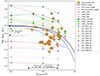 |
Fig. 1. 56Ni mass synthesized during the SN Ia explosion as a function of the progenitor metallicity (Zprogenitor). Our sample of the 34 normal SNe Ia is indicated with orange stars. The analytical TBT03 (solid curved black line) and B10 linear and non-linear (solid and dashed blue lines, respectively) models are overplotted with various SN Ia models we investigated: 3 LN18 near-Mch models (circles with solid lines), 3 LN20 sub-Mch models (squares with dashed lines), and 11 G21 sub-Mch models (diamonds with dash-dotted lines). |
Compared to previous studies, which only used a sample in the sub-solar range, our sample covers the entire Zprogenitor range explored by TBT03:  Z⊙ < Zprogenitor < 3 Z⊙. In this range, most of the Zprogenitor effects occur. Although there is a higher scatter in the derived 56Ni masses compared to the analytical predictions, our sample is within the 56Ni mass range expected from various hydrodynamic simulations.
All hydrodynamic simulations and models of B10 show the same trend as TBT03, but with a different size of the 56Ni mass variation. B10 shows larger variation in the linear and non-linear models because they found a steeper slope than TBT03. The LN18 near-Mch models show a similar variation: ∼24%. However, sub-Mch models show less variation, but similar sizes: ∼15% and ∼17% for LN20 and G21, respectively.
In the following sections and Fig. 2, we investigate the split by models in detail.
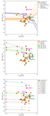 |
Fig. 2. Same as Fig. 1, but the plot is split into the SN Ia models. The top panel shows TBT03 and B10. The solid red line shows the average of 10 000 linear regression results (light red lines) from the LINMIX package, which returns a slope of 0.02 ± 0.03 (0.7σ). The middle panel shows the LN18 and LN20 models, and the bottom panel shows the G21 model. In each panel, we mark four SNe Ia that fit the LN18 and LN20 models well (magenta) and that fit the G21 model (teal). |
3.1.1. TBT03 and B10 models
We investigated the relation between Zprogenitor and the 56Ni mass rather than constraining the progenitors, as discussed by TBT03 and B10 (top panel of Fig. 2). Although some of our sample of SNe Ia follow the trend explored by B10 linear and non-linear models, the scatter in the determined 56Ni mass is higher than is predicted by models, as discussed in previous studies (e.g., H09 and Neill et al. 2009). Since TBT03 and B10 provided equations between Zprogenitor and 56Ni mass, we derived an equation from our sample to compare them. To do this, we performed 10 000 linear regressions on our data using the LINMIX package in Python4, which employs an MCMC posterior sampling and a hierarchical Bayesian approach, considering errors in both variables (Kelly 2007). The LINMIX result shows that the slope of our data is 0.02 ± 0.03 with low statistical significance at 0.7σ. This appears to be the opposite trend to the TBT03 and B10 predictions, but the slope is statistically consistent with zero. We caution that the Zprogenitor range  Z⊙ < Zprogenitor < 4 Z⊙) is too narrow to determine a statistically meaningful result.
3.1.2. LN18 and LN20 models
A first glance at the bottom left panel of Fig. 2 shows a lack of models in the 56Ni mass range lower than 0.6 M⊙. This might be because LN18 and LN20 selected their benchmark models as those that can produce a 56Ni mass of around 0.6 M⊙, considering observations from normal SNe Ia. When we investigated their model setup for the benchmark models (Table 2 of LN18 and Table 1 of LN20), we found that SNe Ia with a 56Ni mass between 0.2 and 0.4 M⊙ can be found when only deflagration is considered for the near-Mch model5 or 0.9 M⊙ with aY-type explosion for the sub-Mch model.
In the figure, we mark two SNe Ia in magenta that appear to be well constrained by the model predictions. SN 2005ag matches the LN18_100 at Zprogenitor = 2 Z⊙ model well. This suggests that its progenitor can be a WD with a total mass of 1.33 M⊙ and Zprogenitor = 2 Z⊙ exploded via the near-Mch DDT mechanism. SN 2004gc can be explained by two models: LN18_500 at 2 Z⊙ and LN20_100-050 at 2 Z⊙. Additional information, such as the 57Ni mass, which can be obtained from SN Ia observations (see e.g., Dimitriadis et al. 2017), is required to distinguish between models.
3.1.3. G21 models
In the bottom right panel of Fig. 2, the G21 models cover a wide range of the 56Ni mass and show a consistent trend with Zprogenitor between them. Our sample is well distributed within the range covered by the models. In particular, many of our SNe Ia are between the G21_09_10 (light green) and G21_09_05 (red) at Zprogenitor > 1 Z⊙ models.
We mark in teal two SNe Ia that that appear to be well constrained by the G21 model. SN 2005el fits the G21_M10_05 at Zprogenitor = 3 Z⊙ model well, while SN 2007ap can be explained by the G21_M09_10 at Zprogenitor = 3 Z⊙ model. Their progenitors are WDs with the same Zprogenitor = 3 Z⊙, but different total masses of 1.05 M⊙ (1.0 M⊙ of Mcore + 0.05 M⊙ of Mshell) and 1.0 M⊙ (0.9 M⊙ of Mcore + 0.10 M⊙ of Mshell), respectively, that exploded via the sub-Mch DD mechanism.
We note that the G21_M10_05 model (orange) and the G21_M10_02 model (green) almost overlap. They show a difference of just 0.01 M⊙ in the 56Ni mass at Zprogenitor = 3 Z⊙. This might be due to the different configurations of the models, but a detailed analysis of this is beyond the scope of the present work.
3.1.4. SN Ia progenitors from different models
In the previous sections, we presented for illustrative purposes candidates for progenitors of four SNe Ia in our sample by comparing them to the hydrodynamic simulations of SN Ia models on the 56Ni mass–Zprogenitor diagram. Other SNe Ia in the sample also closely agree with the model predictions by LN18, LN20, and G21. We mainly selected one model that was considered to show a good fit between the data and the model. However, the above four SNe Ia can apparently also be explained by other models, which have different configurations. Thus, we consider additional models in this section. Table 2 summarizes them.
-
SN 2007ap Only the G21_M09_10 at 3 Z⊙ model can explain this SN here. A pure deflagration explosion of a near-Mch WD of LN18 or a DD explosion of 0.9 M⊙ WD of LN20 might also be a progenitor of this SN Ia, however.
-
SN 2005ag The LN18_100 at 2 Z⊙ model fits this SN Ia well. SN 2005ag is close to the line connecting the G21_M10_10 at 1 Z⊙ model and that at 3 Z⊙. This means that a progenitor of SN 2005ag also can be determined by G21_M10_10 at 2 Z⊙.
-
SN 2005el The G21_M10_05 at 3 Z⊙ model describes this SN Ia best. The LN18_500 at 3 Z⊙ model might also conceivably explain this SN.
-
SN 2004gc For this SN Ia, we selected two models: LN18_500 at 2 Z⊙ and LN20_100-050 at 2 Z⊙. SN 2004gc is on the line connecting G21_M10_03 at 1 Z⊙ model and that at 3 Z⊙.
This section shows that additional observables from SNe Ia or host galaxies to distinguish between models are required, as discussed above. Along with this observational effort, hydrodynamic simulations of SN Ia models with denser grids in the parameter space are needed to fill the gaps between the current models.
Summary of the SN Ia progenitors.
3.2. 56Ni mass as a function of [Fe/H] and [α/Fe]
Weighted-means of 56Ni mass and Hubble residuals in the different environments.
As described in Sect. 2, Zprogenitor was determined from the combination of [Fe/H] and [α/Fe] via Eq. (5). Thus, in order to determine whether [Fe/H] and [α/Fe] also have a trend with the 56Ni mass, we plot the 56Ni mass as a function of [Fe/H] and [α/Fe] in Fig. 3. The TBT03 model is shown in the figure, although the model is described by Zprogenitor. Furthermore, we overplotted the updated TBT03 model by H09. As explained in Sect. 1, H09 accounted for the fact that O/Fe can vary as a function of Fe/H and different populations of stars in the thin disk, the thick disk, and the halo. In the figure, we used Eq. (3), which describes the correlation between the 56Ni mass and [Fe/H]. We note that we placed the x-axis labels at (Fe/H)progenitor/(Fe/H)⊙ and (α/Fe)progenitor/(α/Fe)⊙, instead of [Fe/H] and [α/Fe] to match that of the figures above.
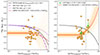 |
Fig. 3. 56Ni mass synthesized during the SN Ia explosion as a function of the progenitor iron abundance ((Fe/H)progenitor) and α-element enrichment ((α/Fe)progenitor). The TBT03 model is plotted as a solid black line, even in the expression of Zprogenitor/Z⊙. The solid red lines show the average of 10 000 linear regression results (light red lines) from the LINMIX package. In the left panel, dot-dashed and dotted purple lines present the TBT03 model, altered for thick- and thin-disk models by H09, respectively. The vertical dashed line in the right panel indicates (α/Fe)progenitor = 0.35, showing a clear gap as discussed by K24. The green squares represent the weighted-means of 56Ni mass in each (α/Fe)progenitor bin. |
In the relation between (Fe/H)progenitor and the 56Ni mass (the left panel of Fig. 3), we obtain a slope of −0.02 ± 0.05 (0.4σ) for our sample using the LINMIX package. This is the same trend as TBT03 and its updated models, but the magnitude of the slope is lower and even consistent with zero when considering the error of the slope. Then, we quantified the goodness of fit based on the reduced χ2 ( ) statistic. Our sample appears to prefer the thick-disk model (
 ) to the thin-disk model (
 ) and the TBT03 model (
 ).
).
Noticeably, for (α/Fe)progenitor, our sample shows the opposite trend to that of the TBT03 model, but we note that this model is expressed in Zprogenitor. We split the sample into two groups based on (α/Fe)progenitor = 0.35, showing a clear gap, and calculated the weighted means of 56Ni mass in each (α/Fe)progenitor bin. The 56Ni mass difference in the different (α/Fe)progenitor groups is 0.12 ± 0.04 (3.0σ) M⊙ (see Table 3). Linear regression using the LINMIX gives the slope of 0.05 ± 0.03 (1.7σ). We caution again that the ranges of (Fe/H)progenitor/(Fe/H)⊙ and (α/Fe)progenitor/(α/Fe)⊙ are too narrow to determine the statistically meaningful result for the LINMIX linear regression. However, the difference in the weighted means of the 56Ni mass in the different (α/Fe)progenitor groups is statistically significant at the 3σ confidence level.
3.3. Zprogenitor versus the Hubble residual
Some previous studies investigated the dependence of a corrected SNe Ia luminosity after the standard light-curve corrections on the currently observed gas-phase or stellar metallicity of the host galaxies (e.g. Gallagher et al. 2005; H09; Childress et al. 2013; Pan et al. 2014; Moreno-Raya et al. 2018; Kang et al. 2020; Galbany et al. 2022; Millán-Irigoyen et al. 2022). In contrast to the well-established host mass-step (Kelly et al. 2010; Lampeitl et al. 2010; Sullivan et al. 2010), it is not yet well established whether a dependence of the SNe Ia luminosity on the host galaxy metallicity exists. K24 discussed that the environmental dependence studies using the currently observed status of the host galaxies might result in a weak correlation between the SN Ia properties and the host galaxy properties because 1) the currently observed status of the host galaxies typically used in previous studies is different from the true SN Ia progenitor star birth environments and because 2) the range of the host galaxy properties is narrower than that of the birth environments of the SN Ia progenitor stars. Because the analytical prediction of TBT03 was performed with Zprogenitor and presented a variation of 0.2 mag in the intrinsic luminosity of SNe Ia, it would be interesting to determine the dependence of a corrected SNe Ia luminosity on Zprogenitor.
In Fig. 4 we investigate the impact of Zprogenitor on the corrected luminosity of SNe Ia, called the Hubble residual (HR ≡ μSN − μz). We note that we did not include a mass-correction term in μSN and an intrinsic scatter term when calculating HRs. This is because we wished to examine which physical property might vary the SN Ia luminosity. For the HR calculation, ΩM = 0.3 and H0 = 70 km s−1 Mpc−1 were used, assuming a flat ΛCDM cosmology. We refer to Kim et al. (2018, 2019) for details of the calculation of μSN and HR.
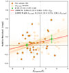 |
Fig. 4. Impact of Zprogenitor on the SN Ia corrected luminosity (i.e. the Hubble residual). Samples with Z of current host galaxies (Zcur, host) are also presented with empty stars. The average of 10 000 linear regression results (light red lines) from the LINMIX package is shown with the solid red line. The LINMIX fit with Zcur, host is indicated with the dashed red line. We split our sample at Zprogenitor = 2.5 (the vertical dashed line), where a gap is shown. The green squares are the weighted means of the HR in the different Zprogenitor group. |
We performed 10 000 linear regressions for our data with the LINMIX package. In addition, we split our sample into two Zprogenitor groups at Zprogenitor = 2.5, where a gap is shown, and we then estimated the weighted means of HRs in each group. The slope of our data is 0.06 ± 0.05 (1.2σ), and the difference in the weighted-means of HRs is 0.14 ± 0.09 (1.6σ) mag (see Table 3). Both results show that SNe Ia from higher-metallicity progenitor stars are fainter than those from lower-metallicity progenitor stars after the light-curve corrections. This trend is inconsistent with the previous studies using current host galaxy properties (e.g., H09; Pan et al. 2014; Millán-Irigoyen et al. 2022). When we used Z of current host galaxies, we still found the opposite trend to previous studies, but the same trend with our Zprogenitor result and also the same size in the 56Ni mass difference but split the sample at 3.5 Z⊙.
4. Discussion and conclusions
We presented the effect of the progenitor star property on the SN Ia intrinsic (i.e. 56Ni mass) and corrected luminosity (i.e. HR). To do this, we tried to reproduce the analytical model of TBT03 and its updated models by H09 and B10, which explored the correlation between the progenitor metallicity and the 56Ni mass synthesized in SNe Ia during the explosion. Moreover, we attempted to constrain the SN Ia progenitors by comparing our data with recent SN Ia explosion simulations on this correlation. Different from the previous studies that used the gas-phase metallicity inferred from the stellar mass of the host galaxies, we used 34 total metallicities of the birth environments of the normal SN Ia progenitor stars determined by K24, assuming that this metallicity can be considered Zprogenitor.
Our sample is well distributed over the Zprogenitor range indicated by TBT03 ( Z⊙ < Zprogenitor < 3 Z⊙), where most of the Zprogenitor effect occurs, compared to previous studies, which only used a sample in the sub-solar range. Our sample shows a higher scatter in the derived 56Ni masses compared to those predicted by the analytical models. Linear regression using the LINMIX package gives a slope of 0.02 ± 0.03 for our sample, which is the opposite trend to the TBT03 and B10 predictions. However, the statistical significance of our slope is low at 0.7σ and thus, the slope is consistent with zero.
Then, we presented three hydrodynamic simulations of SN Ia explosion models: the near-Mch DDT model of LN18, the sub-Mch DD model of LN20, and the sub-Mch DD model of G21. All simulations showed the same trend with TBT03, but the magnitudes of 56Ni mass variations were different. By comparing our sample to those SN Ia explosion simulations on the Zprogenitor–56Ni mass diagram, we tried to constrain four progenitors that fit the result from the simulations well. In the present work, SN 2007ap can be explained by only one model (G21_M09_10 at 3 Z⊙ model), and the other three SNe Ia (SN 2005ag, SN 2005el, and SN 2004gc) fits two or three different models. This means that additional observables of SNe Ia (e.g. the 57Ni mass) and hydrodynamic simulations with denser grids in the parameter space are required to distinguish and to cover the gaps between the models.
We also investigated relations with various other chemical abundances of the progenitor: (Fe/H)progenitor and (α/Fe)progenitor. Regarding (Fe/H)progenitor, our sample appears to follow the same trend as TBT03 and its updated models by H09. The magnitude of the slope is lower, however: −0.02 ± 0.05 (0.4σ) of our sample versus −0.057 of the analytical TBT03 model. Our sample seems to favour the updated TBT03 model altered for thick-disk O/Fe by H09 ( ), in contrast to the previous discussion of H09 and Neill et al. (2009), who discussed this in terms of the thin-disk model (
 ). Our sample preference for the thick disk is somewhat expected because the early-type galaxies we used typically show an enhanced [α/Fe] (e.g., Thomas et al. 2005), as the thick disk exhibits a higher [α/Fe] ratio than the thin disk (e.g., Matteucci 2021, and references therin).
Interestingly, with (α/Fe)progenitor, our sample shows the opposite trend to the TBT03 model. The LINMIX package returns a slope of 0.05 ± 0.03 (1.7σ). Because of the gap at (α/Fe)progenitor = 0.35, we split our sample into two groups and calculated the weighted means of the 56Ni mass in each (α/Fe)progenitor group. We found that the 56Ni mass difference in the different (α/Fe)progenitor groups is 0.12 ± 0.04 (3.0σ) M⊙.
Lastly, we presented the impact of Zprogenitor on the corrected SN Ia luminosity. When we split our sample into two Zprogenitor groups, the difference in the corrected luminosity in each group was 0.14 ± 0.09 mag (1.6σ). Linear regression showed that our sample has a slope of 0.05 ± 0.06 (0.8σ). Our result is that SNe Ia from higher-metallicity progenitor stars are fainter than those from lower-metallicity progenitor stars after the light-curve corrections (in terms of HRs).
If the analytical model is confirmed with more data, we expect that Zprogenitor alone, which can vary the luminosity about 0.2 mag, cannot fully explain the observed scatter in the peak luminosity of SNe Ia (0.5 mag in B and V-bands). In addition, as suggested by the luminosity variation of SNe Ia in the different Zprogenitor group (0.14 ± 0.09 mag), the light-curve standardization process cannot fully account for the progenitor metallicity effect on the luminosity variation. Through this standardization process, the luminosity variation is expected to decrease by ∼30%, from 0.2 mag to 0.14 mag. Other properties, such as the progenitor age, mass, and other chemical elements, will also contribute to the scatter. Furthermore, different explosion scenarios such as a single-degenerate or double-degenerate scenario, deflagration or detonation, and near- or sub-Mch, might produce a dispersion in the peak magnitudes of SNe Ia (see Liu et al. 2023; Ruiter & Seitenzahl 2025, for reviews on SN Ia explosions).
Noticeably, α/Fe appears to play an interesting role in the SN Ia explosion. In this work, the correlation between (α/Fe)progenitor and the 56Ni mass (the right panel of Fig. 3) shows the opposite trend to the TBT03 model, which is expressed in Zprogenitor, however. As reported by K24, [α/Fe] of the SN Ia progenitor star birth environment can clearly distinguish the SN Ia sample into two groups. In the galaxy study, [α/Fe] is linked with the timescale of the star formation history (Δt), such that [α/Fe] ∼  (Thomas et al. 2005; de La Rosa et al. 2011). Thus, a high-[α/Fe] value would result from a concentrated burst of star formation. Consequently, in the high-[α/Fe] environment, a relatively younger SN Ia progenitor will form. Nicolas et al. (2021) and Ginolin et al. (2025) showed that when an SN Ia explodes in younger environments, which are more likely to have a younger progenitor star, the value of x1 is higher than in older environments. When we consider the correlation between x1 and 56Ni mass (Eq. (6)), this progenitor in the high-[α/Fe] environment will likely produce a higher 56Ni mass. However, no studies have been made of the impact of (α/Fe)progenitor on the SN Ia luminosity, while some theoretical studies investigated the impact of the progenitor star metallicity on the SN Ia luminosity (e.g. TBT03, Kasen et al. 2009). Hence, it would be an interesting test to explore the effect of (α/Fe)progenitor on the SN Ia explosion.
Our finding in the relation between Zprogenitor and HR is inconsistent with previous studies using host galaxy metallicities. Previous studies mainly used the currently observed status of host galaxies, which might be different from the progenitor star environments. In addition, previous studies typically used the gas-phase metallicity (O/H) inferred from the stellar mass of the host galaxies, not Zprogenitor. It is also known that the light-curve standardization process over-corrects the brightness of SNe Ia. Therefore, our result using Zprogenitor are probably more robust. However, we need more data to confirm our findings.
We expect more data to come from ongoing and upcoming surveys, such as the Zwicky Transient Facility (ZTF; Bellm et al. 2019; Graham et al. 2019) and the Rubin Observatory’s Legacy Survey of Space and Time (LSST Science Collaboration 2009). ZTF SN Ia DR2 released 3628 spectroscopically classified SNe Ia at z < 0.3 (Rigault et al. 2025). 2663 SNe Ia (out of 3628) passed the basic cuts for cosmological measurements. We expect that half of them will explode in early-type or passive host galaxies (see Rigault et al. 2020, for the rate of SNe Ia at z < 0.1). This means we will have O(103) SNe Ia and host galaxies. This number will be enough to obtain statistically significant results.
A holistic approach (from the SN Ia progenitor star to the explosion with host galaxy analysis and the SN Ia observation) to understand the scatter in the SN Ia luminosity and, thus, the underlying physics of SNe Ia is required to use SNe Ia as more accurate and precise standard candles. This holistic understanding of the luminosity variation of SNe Ia in different environments or from different populations will provide an astrophysical solution to the Hubble tension. For example, considering the SNe Ia in different environments (e.g. locally star-forming versus locally passive), which show a difference of 0.094 ± 0.025 mag in their corrected luminosity, Rigault et al. (2015) found a value of H0 = 70.6 ± 2.6 km s−1 Mpc−1. This value agrees with the Planck measurement of H0 = 67.4 ± 0.5 km s−1 Mpc−1 (Planck Collaboration VI 2020).
Here, we are using the standard notation: [A/B]≡log10(A/B)−log10(A/B)⊙.
It is worth to note that models with deflagration only are aimed at reproducing the peculiar Type Iax SNe class (e.g., Kromer et al. 2015).
Acknowledgments
We would like to thank the referee for the careful reading of the manuscript and for many constructive suggestions, which significantly expanded the manuscript. Y.-L.K. was supported by the Lee Wonchul Fellowship, funded through the BK21 Fostering Outstanding Universities for Research (FOUR) Program (grant No. 4120200513819) and the National Research Foundation of Korea to the Center for Galaxy Evolution Research (RS-2022-NR070872, RS-2022-NR070525). C.C. was supported by Basic Science Research Program through the National Research Foundation of Korea (NRF) funded by the Ministry of Education (RS-2022-NR070872) and by the National Research Foundation of Korea (NRF) grant funded by the Korea government (MSIT) (RS-2022-NR070525). Y.C.K. was supported by Basic Science Research Program through the National Research Foundation of Korea (NRF) funded by the Ministry of Education, Science and Technology (NRF-2017R1D1A1B05028009). This work used pandas(McKinney 2010), numpy(Harris et al. 2020), and matplotlib(Hunter 2007). We also use uncertainties: a Python package for calculations with uncertainties, Eric O. LEBIGOT, http://pythonhosted.org/uncertainties/ and the LINMIX package https://github.com/jmeyers314/linmix/.
References
- Arnett, W. D. 1979, ApJ, 230, L37 [NASA ADS] [CrossRef] [Google Scholar]
- Arnett, W. D. 1982, ApJ, 253, 785 [Google Scholar]
- Asplund, M., Grevesse, N., & Sauval, A. J. 2005, Cosmic Abundances as Records of Stellar Evolution and Nucleosynthesis, 336, 25 [NASA ADS] [Google Scholar]
- Bellm, E. C., Kulkarni, S. R., Graham, M. J., et al. 2019, PASP, 131, 018002 [Google Scholar]
- Bravo, E., Domínguez, I., Badenes, C., et al. 2010, ApJ, 711, L66 [NASA ADS] [CrossRef] [Google Scholar]
- Childress, M., Aldering, G., Antilogus, P., et al. 2013, ApJ, 770, 108 [Google Scholar]
- Chung, C., Yoon, S.-J., Lee, S.-Y., et al. 2013, ApJS, 204, 3 [NASA ADS] [CrossRef] [Google Scholar]
- Cid Fernandes, R., Mateus, A., Sodré, L., et al. 2005, MNRAS, 358, 363 [CrossRef] [Google Scholar]
- Colgate, S. A., & McKee, C. 1969, ApJ, 157, 623 [NASA ADS] [CrossRef] [Google Scholar]
- de La Rosa, I. G., La Barbera, F., Ferreras, I., et al. 2011, MNRAS, 418, L74 [NASA ADS] [CrossRef] [Google Scholar]
- DESI Collaboration (Abdul-Karim, M., et al.) 2025, Phys. Rev. D, 112, 083515 [Google Scholar]
- Dimitriadis, G., Sullivan, M., Kerzendorf, W., et al. 2017, MNRAS, 468, 3798 [NASA ADS] [CrossRef] [Google Scholar]
- Galbany, L., Smith, M., Duarte Puertas, S., et al. 2022, A&A, 659, A89 [NASA ADS] [CrossRef] [EDP Sciences] [Google Scholar]
- Gallagher, J. S., Garnavich, P. M., Berlind, P., et al. 2005, ApJ, 634, 210 [NASA ADS] [CrossRef] [Google Scholar]
- Ginolin, M., Rigault, M., Smith, M., et al. 2025, A&A, 695, A140 [NASA ADS] [CrossRef] [EDP Sciences] [Google Scholar]
- Graham, M. J., Kulkarni, S. R., Bellm, E. C., et al. 2019, PASP, 131, 078001 [Google Scholar]
- Gronow, S., Côté, B., Lach, F., et al. 2021, A&A, 656, A94 [NASA ADS] [CrossRef] [EDP Sciences] [Google Scholar]
- Guy, J., Astier, P., Baumont, S., et al. 2007, A&A, 466, 11 [NASA ADS] [CrossRef] [EDP Sciences] [Google Scholar]
- Guy, J., Sullivan, M., Conley, A., et al. 2010, A&A, 523, A7 [NASA ADS] [CrossRef] [EDP Sciences] [Google Scholar]
- Harris, C. R., Millman, K. J., van der Walt, S. J., et al. 2020, Nature, 585, 357 [NASA ADS] [CrossRef] [Google Scholar]
- Howell, D. A., Sullivan, M., Brown, E. F., et al. 2009, ApJ, 691, 661 [Google Scholar]
- Hunter, J. D. 2007, CSE, 9, 90 [Google Scholar]
- Kang, Y., Kim, Y.-L., Lim, D., et al. 2016, ApJS, 223, 7 [Google Scholar]
- Kang, Y., Lee, Y.-W., Kim, Y.-L., et al. 2020, ApJ, 889, 8 [Google Scholar]
- Kasen, D., Röpke, F. K., & Woosley, S. E. 2009, Nature, 460, 869 [Google Scholar]
- Kelly, B. C. 2007, ApJ, 665, 1489 [Google Scholar]
- Kelly, P. L., Hicken, M., Burke, D. L., et al. 2010, ApJ, 715, 743 [Google Scholar]
- Kim, Y.-L., Smith, M., Sullivan, M., et al. 2018, ApJ, 854, 24 [Google Scholar]
- Kim, Y.-L., Kang, Y., & Lee, Y.-W. 2019, J. Korean Astron. Soc., 52, 181 [Google Scholar]
- Kim, Y.-L., Galbany, L., Hook, I., et al. 2024, MNRAS, 529, 3806 [CrossRef] [Google Scholar]
- Kobayashi, C., Leung, S.-C., & Nomoto, K. 2020, ApJ, 895, 138 [CrossRef] [Google Scholar]
- Kromer, M., Ohlmann, S. T., Pakmor, R., et al. 2015, MNRAS, 450, 3045 [NASA ADS] [CrossRef] [Google Scholar]
- Lampeitl, H., Smith, M., Nichol, R. C., et al. 2010, ApJ, 722, 566 [Google Scholar]
- Lee, H., Skillman, E. D., Cannon, J. M., et al. 2006, ApJ, 647, 970 [NASA ADS] [CrossRef] [Google Scholar]
- Leung, S.-C., & Nomoto, K. 2018, ApJ, 861, 143 [Google Scholar]
- Leung, S.-C., & Nomoto, K. 2020, ApJ, 888, 80 [Google Scholar]
- Liu, Z.-W., Röpke, F. K., & Han, Z. 2023, Res. Astron. Astrophys., 23, 082001 [CrossRef] [Google Scholar]
- LSST Science Collaboration (Abell, P. A., et al.) 2009, ArXiv e-prints [arXiv:0912.0201] [Google Scholar]
- Matteucci, F. 2021, A&ARv, 29, 5 [NASA ADS] [CrossRef] [Google Scholar]
- McKinney, W. 2010, Proceedings of the 9th Python in Science Conference, 56 [Google Scholar]
- Millán-Irigoyen, I., del Valle-Espinosa, M. G., Fernández-Aranda, R., et al. 2022, MNRAS, 517, 3312 [Google Scholar]
- Moreno-Raya, M. E., Mollá, M., López-Sánchez, Á. R., et al. 2016, ApJ, 818, L19 [NASA ADS] [CrossRef] [Google Scholar]
- Moreno-Raya, M. E., Galbany, L., López-Sánchez, Á. R., et al. 2018, MNRAS, 476, 307 [NASA ADS] [CrossRef] [Google Scholar]
- Neill, J. D., Sullivan, M., Howell, D. A., et al. 2009, ApJ, 707, 1449 [Google Scholar]
- Nicolas, N., Rigault, M., Copin, Y., et al. 2021, A&A, 649, A74 [NASA ADS] [CrossRef] [EDP Sciences] [Google Scholar]
- Palla, M. 2021, MNRAS, 503, 3216 [Google Scholar]
- Pan, Y.-C., Sullivan, M., Maguire, K., et al. 2014, MNRAS, 438, 1391 [Google Scholar]
- Perlmutter, S., Aldering, G., Goldhaber, G., et al. 1999, ApJ, 517, 565 [Google Scholar]
- Phillips, M. M. 1993, ApJ, 413, L105 [Google Scholar]
- Planck Collaboration VI. 2020, A&A, 641, A6 [NASA ADS] [CrossRef] [EDP Sciences] [Google Scholar]
- Ramírez, I., Allende Prieto, C., & Lambert, D. L. 2007, A&A, 465, 271 [NASA ADS] [CrossRef] [EDP Sciences] [Google Scholar]
- Riess, A. G., Filippenko, A. V., Challis, P., et al. 1998, AJ, 116, 1009 [Google Scholar]
- Riess, A. G., Yuan, W., Macri, L. M., et al. 2022, ApJ, 934, L7 [NASA ADS] [CrossRef] [Google Scholar]
- Rigault, M., Aldering, G., Kowalski, M., et al. 2015, ApJ, 802, 20 [Google Scholar]
- Rigault, M., Brinnel, V., Aldering, G., et al. 2020, A&A, 644, A176 [NASA ADS] [CrossRef] [EDP Sciences] [Google Scholar]
- Rigault, M., Smith, M., Goobar, A., et al. 2025, A&A, 694, A1 [NASA ADS] [CrossRef] [EDP Sciences] [Google Scholar]
- Ruiter, A. J., & Seitenzahl, I. R. 2025, A&ARv, 33, 1 [Google Scholar]
- Scalzo, R. A., Parent, E., Burns, C., et al. 2019, MNRAS, 483, 628 [Google Scholar]
- Sullivan, M., Conley, A., Howell, D. A., et al. 2010, MNRAS, 406, 782 [NASA ADS] [Google Scholar]
- Thomas, D., Maraston, C., Bender, R., et al. 2005, ApJ, 621, 673 [NASA ADS] [CrossRef] [Google Scholar]
- Timmes, F. X., Brown, E. F., & Truran, J. W. 2003, ApJ, 590, L83 [Google Scholar]
- Tremonti, C. A., Heckman, T. M., Kauffmann, G., et al. 2004, ApJ, 613, 898 [Google Scholar]
- Tripp, R. 1998, A&A, 331, 815 [NASA ADS] [Google Scholar]
- Trueman, T. C. L., Pignatari, M., Cseh, B., et al. 2025, A&A, 696, A164 [NASA ADS] [CrossRef] [EDP Sciences] [Google Scholar]
- Truran, J. W., Arnett, W. D., & Cameron, A. G. W. 1967, Can. J. Phys., 45, 2315 [NASA ADS] [CrossRef] [Google Scholar]
- Walcher, C. J., Coelho, P. R. T., Gallazzi, A., et al. 2015, A&A, 582, A46 [NASA ADS] [CrossRef] [EDP Sciences] [Google Scholar]
Appendix A: Correlation between Zprogenitor and (Fe/H)progenitor and (α/Fe)progenitor
In the present work, we derived Zprogenitor from (Fe/H)progenitor and (α/Fe)progenitor via Eq. 1. Here, to see this visually, we plot the correlation between Zprogenitor, (Fe/H)progenitor and (α/Fe)progenitor for our sample in Fig. A.1. Up to 2 Z⊙, they appear to be a one-to-one relation, but in the higher metallicity region, they show a large scatter. In the figure, each point represents not only the SN Ia progenitor star but also the birth environment of the progenitor star. Moreover, by the definition of K24, each point also indicates a whole galaxy at 0 Gyr old. A detailed analysis and interpretation of this trend is beyond the scope of the present work, but would be of interest to the extragalactic community.
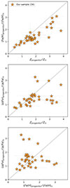 |
Fig. A.1. Correlation between Zprogenitor, (Fe/H)progenitor and (α/Fe)progenitor for our sample. Dashed lines indicate a one-to-one relation. |
All Tables
All Figures
|
Fig. 1. 56Ni mass synthesized during the SN Ia explosion as a function of the progenitor metallicity (Zprogenitor). Our sample of the 34 normal SNe Ia is indicated with orange stars. The analytical TBT03 (solid curved black line) and B10 linear and non-linear (solid and dashed blue lines, respectively) models are overplotted with various SN Ia models we investigated: 3 LN18 near-Mch models (circles with solid lines), 3 LN20 sub-Mch models (squares with dashed lines), and 11 G21 sub-Mch models (diamonds with dash-dotted lines). |
| In the text | |
|
Fig. 2. Same as Fig. 1, but the plot is split into the SN Ia models. The top panel shows TBT03 and B10. The solid red line shows the average of 10 000 linear regression results (light red lines) from the LINMIX package, which returns a slope of 0.02 ± 0.03 (0.7σ). The middle panel shows the LN18 and LN20 models, and the bottom panel shows the G21 model. In each panel, we mark four SNe Ia that fit the LN18 and LN20 models well (magenta) and that fit the G21 model (teal). |
| In the text | |
|
Fig. 3. 56Ni mass synthesized during the SN Ia explosion as a function of the progenitor iron abundance ((Fe/H)progenitor) and α-element enrichment ((α/Fe)progenitor). The TBT03 model is plotted as a solid black line, even in the expression of Zprogenitor/Z⊙. The solid red lines show the average of 10 000 linear regression results (light red lines) from the LINMIX package. In the left panel, dot-dashed and dotted purple lines present the TBT03 model, altered for thick- and thin-disk models by H09, respectively. The vertical dashed line in the right panel indicates (α/Fe)progenitor = 0.35, showing a clear gap as discussed by K24. The green squares represent the weighted-means of 56Ni mass in each (α/Fe)progenitor bin. |
| In the text | |
|
Fig. 4. Impact of Zprogenitor on the SN Ia corrected luminosity (i.e. the Hubble residual). Samples with Z of current host galaxies (Zcur, host) are also presented with empty stars. The average of 10 000 linear regression results (light red lines) from the LINMIX package is shown with the solid red line. The LINMIX fit with Zcur, host is indicated with the dashed red line. We split our sample at Zprogenitor = 2.5 (the vertical dashed line), where a gap is shown. The green squares are the weighted means of the HR in the different Zprogenitor group. |
| In the text | |
|
Fig. A.1. Correlation between Zprogenitor, (Fe/H)progenitor and (α/Fe)progenitor for our sample. Dashed lines indicate a one-to-one relation. |
| In the text | |
Current usage metrics show cumulative count of Article Views (full-text article views including HTML views, PDF and ePub downloads, according to the available data) and Abstracts Views on Vision4Press platform.
Data correspond to usage on the plateform after 2015. The current usage metrics is available 48-96 hours after online publication and is updated daily on week days.
Initial download of the metrics may take a while.