| Issue |
A&A
Volume 703, November 2025
|
|
|---|---|---|
| Article Number | A106 | |
| Number of page(s) | 21 | |
| Section | Extragalactic astronomy | |
| DOI | https://doi.org/10.1051/0004-6361/202555372 | |
| Published online | 13 November 2025 | |
Insights on metal enrichment and environmental effects at z ≈ 5–7 with JWST ASPIRE/EIGER and the chemical evolution model
1
Cosmic Dawn Center (DAWN), Denmark
2
Niels Bohr Institute, University of Copenhagen, Jagtvej 128, DK2200 Copenhagen N, Denmark
3
Department of Astronomy, Tsinghua University, Beijing 100084, China
4
Center for Astrophysics and Planetary Science, Racah Institute of Physics, The Hebrew University, Jerusalem 91904, Israel
5
Santa Cruz Institute for Particle Physics, University of California, Santa Cruz, CA 95064, USA
6
Steward Observatory, University of Arizona, 933 North Cherry Avenue, Tucson, AZ 85721-0065, USA
7
International Gemini Observatory/NSF NOIRLab, 670 N A’ohoku Place, Hilo, Hawai’i 96720, USA
8
Department of Physics, Northwestern College, 101 7th Street SW, Orange City, Iowa 51041, USA
9
Center for Astrophysics | Harvard & Smithsonian, 60 Garden St., Cambridge, MA 02138, USA
10
LUX, Observatoire de Paris, Université PSL, Sorbonne Université, CNRS, 77 Av. Denfert-Rochereau, F-75014 Paris, France
11
Max Planck Institut für Astronomie, Königstuhl 17, D-69117 Heidelberg, Germany
12
Department of Astronomy, University of Michigan, 1085 S. University Avenue, Ann Arbor, MI 48109, USA
13
Department of Astronomy, Huazhong University of Science and Technology, Wuhan, Hubei 430074, China
14
Chinese Academy of Sciences South America Center for Astronomy, National Astronomical Observatories, CAS, Beijing 100101, China
15
Departamento de Astronomía, Universidad de Chile, Casilla 36-D, Santiago, Chile
⋆ Corresponding author: This email address is being protected from spambots. You need JavaScript enabled to view it.
Received:
2
May
2025
Accepted:
16
September
2025
Abstract
We present the mass–metallicity relation (MZR) for a parent sample of 604 galaxies at z = 5.34 − 6.94 with [O III] doublets detected that was obtained from the deep JWST/NIRCam wide field slitless spectroscopic (WFSS) observations in 26 quasar fields. The sample incorporates the full observations of 25 quasar fields from the JWST Cycle 1 GO program ASPIRE and the quasar SDSS J0100+2802 from the JWST EIGER program. We identified 204 galaxies residing in overdense structures using the friends-of-friends (FoF) algorithm. We estimated the electron temperature of 2.0+0.3−0.4 × 10⁴ K from the Hγ and [O III]4363 lines in the stacked spectrum, indicating a metal-poor sample with a median gas phase metallicity of 12 + log(O/H) = 7.65+0.26−0.15. With the most up-to-date strong line calibration based on NIRSpec observations, we find that the MZR shows a metal enhancement of ∼0.2 dex at the high mass end in overdense environments. However, compared to the local fundamental metallicity relation (FMR), our galaxy sample at z > 5 shows a metal deficiency of ∼0.2 dex relative to FMR predictions. We explain the observed trend of FMR with a simple analytical model, and we favor dilution from intense gas accretion over outflow to explain the metallicity properties at z > 5. The high-redshift galaxies are likely in a rapid gas accretion phase when their metal and gas contents are in a non-equilibrium state. According to model predictions, the protocluster members are closer to the gas equilibrium state than field galaxies and thus have a higher metallicity and are closer to the local FMR. Our results suggest that the accelerated star formation during protocluster assembly likely plays a key role in shaping the observed MZR and FMR, indicating a potentially earlier onset of metal enrichment in overdense environments at z ≈ 5 − 7.
Key words: ISM: abundances / galaxies: clusters: general / galaxies: evolution / galaxies: formation / galaxies: high-redshift
© The Authors 2025
 Open Access article, published by EDP Sciences, under the terms of the Creative Commons Attribution License (https://creativecommons.org/licenses/by/4.0), which permits unrestricted use, distribution, and reproduction in any medium, provided the original work is properly cited.
This article is published in open access under the Subscribe to Open model. This email address is being protected from spambots. You need JavaScript enabled to view it. to support open access publication.
1. Introduction
The gas-phase metallicity (hereafter referred to as “metallicity” for simplicity) of galaxies represents the current state of chemical enrichment, and it bears the imprints of both internal and external effects such as star formation, gas accretion, feedback, and mergers. While the star-formation density peaks at cosmic noon (Madau & Dickinson 2014), studying galaxies at the Epoch of Reionization provides a more complete picture of the earlier evolution of galaxies.
The metallicity of a galaxy has been found to be highly correlated with its stellar mass, i.e., mass–metallicity relation (MZR), across a wide mass range (106 − 1011 M⊙) and a wide redshift range (from z = 0 to z ≳ 6) (Tremonti et al. 2004; Maiolino et al. 2008; Andrews & Martini 2013; Zahid et al. 2014; Curti et al. 2020; Sanders et al. 2021; Henry et al. 2021; Nakajima et al. 2023; Langeroodi et al. 2023; Stephenson et al. 2024; Pallottini et al. 2025). The origin of MZR is still under debate. Many works have explored the various origins of the MZR, such as inflow and outflow properties (Erb et al. 2006; Finlator & Davé 2008; Spitoni et al. 2010; Bassini et al. 2024; Pérez-Díaz et al. 2024), secular evolution (Somerville & Davé 2015), stellar age (Duarte Puertas et al. 2022), and active galactic nucleus (AGN) activity (Thomas et al. 2019). A common interpretation within the outflow and inflow scenarios is that outflow efficiency decreases with increasing gravitational potential, thus increasing the metal retention for massive galaxies (Finlator & Davé 2008). In contrast, Baker & Maiolino (2023) argued that the MZR arises because the stellar mass is proportional to the total metal production in a galaxy rather than due to more massive galaxies retaining metals more efficiently.
On the other hand, observations have revealed that the MZR is not universal and can vary with the environment. This type of influence on a galaxy’s evolution is known as an environmental effect, and it manifests in many different forms, such as ram pressure stripping and strangulation (McCarthy et al. 2008; Peng et al. 2015; Boselli et al. 2022; Xu et al. 2025a), mergers (Brennan et al. 2015; Delahaye et al. 2017), harassment (Boselli & Gavazzi 2006; Bialas et al. 2015), and preprocessing (Fujita 2004; Werner et al. 2022; Lopes et al. 2024). The local galaxy clusters host galaxy populations with varied properties (Murphy et al. 2009; Bahé et al. 2013), and such environmental effects are also found at higher redshifts up to z ≳ 2 (Hatch et al. 2017; Tadaki et al. 2019; Namiki et al. 2019; Wang et al. 2022; Lemaux et al. 2022; Liu et al. 2023; Pérez-Martínez et al. 2023; Hughes et al. 2025; Forrest et al. 2024).
However, the environmental impact on the MZR at high redshifts-particularly within the first gigayear after the Big Bang-remains uncertain, with mixed observational evidence and different theoretical interpretations. While some studies have found metal-deficient galaxies in overdense environments at z ∼ 2, such as Valentino et al. (2015) in the CL J1449+0856 cluster at z = 1.99, Li et al. (2022) and Wang et al. (2022) in the BOSS1244 protocluster at z = 2.24, and Pérez-Martínez et al. (2024) at z = 2.53, others have reported metal enhancement in protoclusters in similar redshifts. For example, Shimakawa et al. (2015) found the MZR to be systematically shifted upward by ≳0.1 dex in two rich protoclusters compared to coeval field galaxies, and Shimakawa et al. (2018) reported enhanced galaxy formation in the densest regions of a protocluster at z = 2.5. Pérez-Martínez et al. (2023) found a mild metal enhancement in the Spiderweb protocluster at z = 2.16, consistent with a scenario of efficient gas recycling and confinement due to the external intracluster medium (ICM) pressure. Similarly, Adachi et al. (2025,) found 0.08 − 0.15 dex metal enhancement in the X-ray cluster XCS2215 at z = 1.46, and they also attributed this to the confinement of gas by ICM pressure.
Conversely, Calabrò et al. (2022) observed a metallicity deficit of ∼0.1 dex in overdense regions at 2 < z < 4, and Sattari et al. (2021) also found metal-deficient populations in dense environments. Some studies have also suggested less environmental impact on the MZR. For instance, Namiki et al. (2019) found no significant differences in the MZR for a cluster at z = 1.52 compared with the field. However, the observed differences reported in those works may well arise from measurement uncertainties, as the typical offsets of ∼0.1 dex are comparable to the uncertainties.
Hydrodynamical simulations are also starting to be used to explore this complexity (Fukushima et al. 2023; Esposito et al. 2025; Morokuma-Matsui et al. 2025). For example, Wang et al. (2023b) employed the EAGLE simulation (Crain et al. 2015) and reported strong environmental influences on the MZR at both z = 0 and z > 2, attributing them to both gas accretion and gas stripping. These results suggest that metallicity evolution may depend on both local physical processes, such as cold-mode accretion-driven gas dilution (e.g., Wang et al. 2022), and external processes, such as recycling-driven enrichment due to external pressure (e.g., Pérez-Martínez et al. 2023). Additional high-redshift observations and simulations are needed to fully understand these environmental influences.
With the recent surge in observations from JWST, an increasing number of high-redshift galaxies have been identified during the Epoch of Reionization. This advancement enables the study of early galaxies using large statistical samples in both field and protocluster environments. The JWST ASPIRE program (A SPectroscopic survey of biased halos In the Reionization Era; program ID 2078, PI: F. Wang) aims to target 25 quasars at z > 6.5 using JWST NIRCam/WFSS with filter F356W while also searching for [O III]+ Hβ emitters at z = 5.34 − 6.94 (Wang et al. 2023a). The JWST EIGER program (Emission-line galaxies and the Intergalactic Gas in the Epoch of Reionization; program ID 1243, PI S. Lilly) targets six quasar fields, each centered on a quasar at 5.98 < z < 7.08 (Kashino et al. 2023). Both ASPIRE and EIGER utilize the F356W filter for NIRCam/WFSS observations, providing identical redshift coverage. These observations have allowed us to identify galaxies in both overdense and field environments in a large survey volume and to reveal the impacts of environments on galaxy formation and evolution at the Epoch of Reionization. Recent JWST observations have unveiled an abundant population of high-redshift overdensities at z ∼ 5 − 6 through the detection of either Hα or [O III] emissions with NIRCam/WFSS and NIRSpec (Laporte et al. 2022; Wang et al. 2023a; Castellano et al. 2023; Kashino et al. 2023; Helton et al. 2024a,b; Sun et al. 2024; Herard-Demanche et al. 2025; Champagne et al. 2025). Helton et al. (2024a) discovered older stellar populations in a z = 5.4 protocluster with JWST that point to earlier star formation and mass assembly in protoclusters, and Champagne et al. (2025) also observed galaxies in a protocluster at z = 6.6 as being more massive and older than field galaxies. Similarly, Morishita et al. (2025a) have found more evolved stellar populations at z ∼ 5.7, which is in agreement with accelerated star formation. Furthermore, Morishita et al. (2023) identified a galaxy protocluster at the redshift z = 7.9 using JWST NIRSpec, and a significant metallicity scatter was observed within this system, suggesting a rapid gas cycle in overdense regions (Morishita et al. 2025b). Li et al. (2025) observed enhanced dust extinction, weaker Lyman-alpha emission, and/or higher damped Lyman-alpha absorption in protocluster galaxies at redshifts 4.5 < z < 10.
In this paper, we present the first effort to investigate MZR at 5 < z < 7 in both blank fields and overdense environments utilizing a large, homogeneous sample selected through JWSTNIRCam/WFSS observations in the F356W filter. The paper is organized as follows. In Section 2, we describe the observations and data used in our analysis. In Section 3, we present the methodology, including emitter finding and spectra stacking. In Section 4 and 5, we present our main results on MZR and fundamental metallicity relation (FMR). We introduce a simple analytical model in 6, and we compare our observations with an analytical model and simulations in Section 7. In Section 8, we summarize our results and their implications. Throughout this article, we adopt the AB magnitude system and assume a flat ΛCDM cosmology with Ωm = 0.3, ΩΛ = 0.7, and H0 = 70 km s−1 Mpc−1.
2. Observations and data reduction
2.1. NIRCam imaging data reduction
The images were processed in the same way as described in Wang et al. (2023a). Briefly, the reduction was performed using version 1.8.3 of the JWST Calibration Pipeline with the reference files from version 11.16.15 of the standard Calibration Reference Data System. The 1/f noise is removed on a row-by-row and column-by-column basis. We then created a master median background for each combination of detector and filter using all calibrated exposures from stage 2. These master backgrounds were subsequently scaled and subtracted from the individual exposures to remove extra detector-level noise. After Stages 2 and 3, the images were aligned to Gaia DR3 and drizzled to a common pixel scale of 0 031/pixel.
2.2. NIRCam WFSS data reduction
We used version 1.13.4 of the JWST Calibration pipeline CALWEBB Stage 1 to calibrate individual NIRCam WFSS exposures, with reference files jwst_1321.pmap. The 1/f noise is then subtracted along rows for Grism-R exposures using the routine described in Wang et al. (2023a). The world coordinate system (WCS) information is assigned to each exposure with the assign_wcs step. The flat field is done with CALWEBB stage-2. We build the median backgrounds based on all of the WFSS exposures, which are then scaled and subtracted from each individual exposure. The astrometric offsets are measured between each of the short wavelength images and the fully calibrated F356W mosaic to align each grism exposure with the direct image. The WCS alignment ensures the tracing model works properly.
The pre-processed WFSS exposures are then processed by the Grism Redshift & Line Analysis tool (GRIZLI; Brammer et al. 2022). We use the V9 spectral tracing and grism dispersion models1. The detection catalogs for spectral extraction are built from the F356W direct image, and the continuum cross-contamination is subtracted by GRIZLI forward modeling using the F356W image as the reference image for each grism exposure. The 1D spectra are extracted with optimal extraction (Horne 1989) with optimal profiles generated from F356W images and corresponding segmentation maps.
3. Methodology and measurements
3.1. Emitter and overdensity identification
To search for [O III] emitters, we use the automatic line searching algorithm detailed in Wang et al. (2023a) on continuum-subtracted spectra. In brief, we applied a peak finding algorithm to search for all pixels with S/N > 3 and rejected peaks with two neighboring pixels with S/N < 1.5 to avoid likely hot pixels or cosmic ray signals. We then performed a Gaussian fitting to the remaining peaks, and accepted lines with S/N > 5 and FWHM wider than half the spectral resolution and narrower than seven times the spectral resolution. For each detected lines, we assumed that it is [O III] λ 5007 Å, and measure the S/N at the expected wavelength of [O III] λ 4959 Å with the same FWHM as [O III] λ 5007 Å. We regard the [O III] emitter candidates as good if the significance of detection is over 2σ. We then apply a color excess cut from broad band photometry (magF200W − magF356W > 0.2) to further reject candidates that are not likely to be [O III] emitters. We then visually inspect the remaining candidates. We compared the source morphology on direct image and emission lines on 2D spectra, and rejected sources whose emission lines’ shapes are apparently different from the direct image, which are likely to be contaminated by other sources. We also visually check all the sources along the dispersion direction of the candidates to avoid contamination from nearby sources. We finally selected 487 [O III] emitters from 25 fields in ASPIRE. The emitter selection criteria for the EIGER field are outlined in Kashino et al. (2023), and we use the publicly available catalog of 117 [O III] emitters provided by the EIGER collaboration2. The spectra of [O III] emitters are extracted from our reduced products in the SDSS J0100+2802 field, using coordinates from the EIGER collaboration. Finally, the complete sample incorporates 604 [O III] emitters in total. The redshift distribution is shown in Fig. 1.
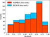 |
Fig. 1. Redshift distribution of the full sample in this work. [O III] emitters from ASPIRE and EIGER programs are marked by red and blue, respectively. The EIGER sample is stacked on top of the ASPIREsample. |
Following Helton et al. (2024a), we used a friends-of-friends (FoF) algorithm to identify overdense structures. This algorithm selects galaxy groups by searching for companions around a central galaxy within a projected separation dlink = 500 kpc and line-of-sight (LOS) velocity σlink = 500 km/s. The algorithm iteratively performs the process above for all the companions identified until no more galaxies are found. Similar to Helton et al. (2024a), we require a minimum number of constituent galaxies (Ngalaxies ≥ 4) as a cluster. We note that these overdensities are not “real” clusters under the standard definition, which describes mature, gravitationally bound structures in virial equilibrium. They may not necessarily be protoclusters either, as it is uncertain whether these systems will ultimately evolve into clusters at z = 0. We refer to them as “clusters” throughout this work for simplicity, as they exhibit greater clustering compared to isolated galaxies. In addition, as protoclusters can span scales of ∼deg (Hung et al. 2025), our selected overdensities on scales of ∼arcmin in each field may only represent some sub-components of a protocluster, without knowing the exact location of the main halo.
We finally identified 204 galaxies in overdense environments (cluster) and 400 galaxies that are not linked to another (field). Among the selected clusters, an extreme overdensity at z = 6.6 in J0305–3150 with δgal = 12.6 has been reported in Wang et al. (2023a). And three major overdensities at z ≈ 6.2, 6.3, 6.8 in the SDSS J0100+2802 field have also been reported in Kashino et al. (2023).
3.2. SED fitting
The spectral energy distribution (SED) modeling of our sample is carried out using the Bayesian code BEAGLE (Chevallard & Charlot 2016), incorporating broadband photometry and [O III] line fluxes as inputs. BEAGLE computes the stellar and nebular emissions based on an updated version of the Bruzual & Charlot (2003) stellar population synthesis models (Gutkin et al. 2016). We adopt a delayed-τ star formation history (SFH), the Small Magellanic Cloud (SMC) dust attenuation law, and a Chabrier initial mass function (IMF) (Chabrier 2003) with an upper mass limit of 100 M⊙. We note that the fitted parameters are sensitive to underlying assumptions, such as SFH, and we discuss the impact of these systematic uncertainties in Section 7.3.
Flat priors in log-space are applied for the characteristic star formation timescale, τ, ranging from 107 to 1010.5 years, and for stellar masses, spanning 104 M⊙ to 1012 M⊙. We place log-uniform priors on stellar metallicity log(Z/Z⊙) from −3 to 0, and ionization parameter log(U) from −4 to −1. The metallicity and ionization parameter ranges are sufficiently broad to encompass the typical values suggested by relevant observations (Strom et al. 2018; Reddy et al. 2023; Trump et al. 2023; Sanders et al. 2024). BEAGLE assumes that total interstellar metallicity, including dust and gas-phase metallicity, is the same as stellar metallicity. The optical depth in the V band is allowed to vary between 0 and 0.5 in log-space. For both the ASPIRE and EIGER fields, we utilize data from three JWST NIRCam bands: F115W, F200W, and F356W.
3.3. Spectra stacking
To enhance the spectral signal-to-noise ratio (S/N), we stack galaxies that are expected to share similar metallicities and, consequently, similar line ratios. Given the strong correlation in the MZR (e.g., Nakajima et al. 2023; Chakraborty et al. 2025; Sarkar et al. 2025), it is reasonable to assume that galaxies with similar stellar masses have similar metallicities. We divided the galaxy sample into two categories: overdense regions (clusters) and blank fields (fields), further stratified into three mass bins. The mass bins were uniformly spaced to ensure comparable S/N in the resulting stacks for each bin. Before stacking, we subtract a polynomial continuum from each spectrum, removing potential background contamination. We resample our spectra to rest-frame on a common 1 Å wavelength grid with flux preserved using spectres (Carnall 2017). Following Wang et al. (2022), to avoid the excessive weighting toward bright sources with stronger line fluxes, we normalized each spectrum by its measured [O III] flux. We take the median value of the normalized spectra at each wavelength grid, and the uncertainty is estimated by measuring the standard deviation from 1000 bootstrap realizations of the sample.
The Hγ and [O III] emission lines at 6.25 < z < 6.95 are redshifted into the F356W filter coverage. Fig. 2 presents the median-stacked 1D rest-frame spectrum for all galaxies within this redshift range. In the stacked spectrum, we detect the [O III] auroral line at a 2σ significance level, enabling us to determine the median metallicity of the full sample using the Te method. We do not further measure Te for subsamples divided into mass bins or field/cluster bins, as these subsamples span redshift ranges broader than 6.25 < z < 6.95, resulting in incomplete spectral coverage. The reduced sample sizes in these bins hinder reliable [O III] measurements; consequently, any observed differences between the samples are more likely driven by random noise than by environmental effects. The analysis is further discussed in Section 4.1.
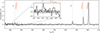 |
Fig. 2. Median stacked 1D rest-frame spectra for our full sample galaxies at z > 6.25, with continuum subtracted. The fluxes are normalized by the peak of [O III]5007 flux after stacking. |
3.4. Flux measurements
For individual targets, we apply GRIZLI to measure line fluxes by forward modeling. This process starts with the construction of a one-dimensional (1D) spectrum, which includes multiple Gaussian-shaped emission lines ([O III] doublets and Hβ) at a given redshift, combined with a continuum derived from sets of empirical spectra (Brammer et al. 2008). This modeled 1D spectrum is then used to generate a two-dimensional (2D) model spectrum, dispersing each pixel from the F356W direct image onto a grism detector frame for each exposure with grism sensitivity and dispersion function. The forward-modeled 2D spectrum is subsequently compared to the observational data, and a χ2-minimization is performed to identify the best-fit coefficients for both the continuum templates and the Gaussian amplitudes. A negative Gaussian amplitude is allowed to account for the effects of random noise. The best-fit emission-line fluxes are derived from the Gaussian components. Since we have required robust detection of [O III] lines in emitter identification, we have all S/N[O III] > 3 in the emitter identification algorithm. However, Hβ is not always detectable due to its faintness. In our subsequent measurements, we set an S/N cut of S/NHβ > 1.5 to ensure spectra quality. In Appendix A, we further quantify the bias of stacking low S/N spectra, leading to an overestimation of [O III]/Hβ ratio.
After stacking, we measure line fluxes from the 1D spectra by fitting a combination of a polynomial continuum and multiple Gaussian emission line components. We note that the continuum is not necessarily physical, as the grism spectra are highly likely to be contaminated by light from nearby sources. Although GRIZLI has subtracted the contamination from bright sources, there are still possible residuals in the grism spectra due to potential tracing offsets. The polynomial continuum further subtracts residuals to ensure robust line flux measurements. We use two separate Gaussian components for the [O III] doublets and find that the line ratios of [O III]5007/[O III]4959 are close to 2.98 : 1. Line fluxes and uncertainties are derived from the uncertainties of their Gaussian components.
In Fig. 3, we show the individual and stacked [O III]/Hβ ratios as a function of stellar mass, and compare them with the mass-excitation demarcation (Coil et al. 2015). We find that none of the galaxies in our sample exceed the AGN criteria at the 1σ confidence level. Thus, they are suitable for metallicity calibration for star-forming galaxies, as we discuss in Section 3.5.
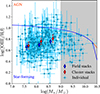 |
Fig. 3. Mass–excitation diagram for our sample galaxies. The blue circles represent individual measurements. The red and blue diamonds represent stacked measurements in cluster and field galaxies, respectively. The blue and orange curves indicate the lower and upper mass-excitation demarcation by Coil et al. (2015). The AGNs (star-forming galaxies) are above (below) the demarcation. The gray shaded region indicates the high-mass end, which we did not analyze due to uncertainties in the metallicity calibrations in this regime. |
3.5. Metallicity measurements
The direct electron temperature (Te) method for determining metallicity relies on collisionally excited emission lines from metal ions. To estimate the electron temperature of doubly ionized oxygen (O++), the intensity ratio of [O III] to [O III]4959,5007 is commonly used. The [O III]4959 and [O III]5007 lines originate from transitions from the 1D energy level to the ground state 3P, while the [O III] line arises from a higher-energy transition from 1S to 1D. The probability of excitation to the 1D and 1S states depends on the collisional rate for each ion, which is proportional to  , where ve represents the electron velocity. Therefore, measuring the emission intensities associated with these [O III] and [O III]5007 transitions allows for an estimate of the electron temperature Te. Likewise, the electron temperature of singly ionized oxygen (O+) can be estimated by the ratio of [O II]7322,7332 and [O II]3726,3729.
Given the electron temperature, metallicity is estimated using the direct method, based on physical conditions, emissivities, and observed fluxes, with photoionization models applied to account for the temperature and ionization structures of H II regions (e.g., Izotov et al. 2006; Pérez-Montero 2017; Amayo et al. 2021).
Due to the challenges of detecting faint [O III], strong emission-line calibration methods have been widely used to determine the metallicity of high-redshift galaxies. These methods rely on the ratios between bright collisionally excited lines (e.g., [O III],[O II] ) and Balmer recombination lines (e.g., Hα, Hβ) to establish metallicity calibrations (Pagel et al. 1979). Since these lines are among the strongest metal lines in the optical spectrum, they are applicable to galaxies across a broad range of redshifts and luminosities. Strong-line calibrations are constructed using samples where [O III] is detected, enabling the establishment of empirical relationships between metallicity measured via the direct Te method and strong emission-line ratios (e.g., [O III]5007/Hβ, [O III]/[O II] ) (Pettini & Pagel 2004). For these calibrations to be reliable, the galaxies used in their derivation should have physical properties similar to those of the target galaxies. Typically, strong-line calibrations are based on galaxies selected from the BPT diagram (Baldwin et al. 1981) that exhibit detectable [O III] emission (e.g., Bian et al. 2018). Therefore, when applying these calibrations, it is essential to ensure that the galaxies share similar ionization mechanisms. In such cases, they often appear in similar regions of the BPT diagram, as a consequence of emissions arising from similar ionizing scenarios.
To improve metallicity measurements of high-redshift galaxies, many strong-line calibrations use high-ionization galaxies in the local universe as high-redshift analogs, and establish empirical relations that represent the ionization conditions for high-redshift galaxies (Bian et al. 2018, hereafter B18, Izotov et al. 2019, hereafter I19, Nakajima et al. 2022, hereafter N22, Curti et al. 2020, hereafter C20). However, these local analogs may not fully represent the ionization conditions of high-redshift galaxies. Kewley et al. (2013) found a significant evolution of emission line ratios toward higher excitation at high-redshift, which is also confirmed by recent JWST observations (Shapley et al. 2023). Thus, more reliable metallicity diagnostics are needed to improve the accuracy of metallicitymeasurements.
For our galaxy sample, we adopt the two most recent metallicity diagnostics (Sanders et al. 2024 hereafter S24, and Chakraborty et al. 2025 hereafter C24). Unlike calibrations that rely on local analogs of high-redshift galaxies (e.g., B18, N22, C20), these diagnostics are derived directly from high-redshift galaxies observed with JWST/NIRSpec. Specifically, they are based on a sample of galaxies at redshifts z = 2 − 9 with detected [O III], allowing for metallicity estimates using the direct Te method. This approach provides a more precise characterization of high-redshift galaxy properties, reducing potential biases introduced by local analog calibrations. However, a limitation of the [O III]/Hβ (R3) diagnostic is that it produces a double-branched solution for a given line ratio. Since [O II]3727 falls outside the spectral coverage of the F356W grism, we adopt the low-metallicity solution with 12 + log(O/H)≲7.9. This assumption is supported by the fact that most galaxies with similar stellar masses at comparable redshifts (z ≥ 6 − 7) have been confirmed as metal-poor using the Te method (Sanders et al. 2024; Curti et al. 2023; Nakajima et al. 2023; Trump et al. 2023; Jones et al. 2023; Chakraborty et al. 2025).
4. The metallicities and mass–metallicity relation
4.1. Direct Te metallicity and empirical calibrations
In Fig. 2, we can detect [O III] and Hγ for median stacked spectra of sample galaxies at z > 6.25, and we can estimate the metallicity using the Te method. We measure the Balmer ratio Hγ/Hβ = 0.44 ± 0.04, consistent with a recent study in the EIGER field (Matthee et al. 2023). Assuming the SMC dust curve, we estimate the dust attenuation as  , suggesting moderate dust in our sample, albeit with considerable uncertainties.
Following Trump et al. (2023), we measured the [O III] ratio with dust attenuation corrected as follows:
![Mathematical equation: $$ \begin{aligned} \frac{[\mathrm{O}{\small { {\text{ III}}}} ]_{4363}}{[\mathrm{O}{\small { {\text{ III}}}} ]_{4959+5007}}=\frac{[\mathrm{O}{\small { {\text{ III}}}} ]_{4363}}{\mathrm{H_\gamma }}\frac{\mathrm{H_\beta }}{[\mathrm{O}{\small { {\text{ III}}}} ]_{4959+5007}} \times (2.1)^{-1}, \end{aligned} $$](/articles/aa/full_html/2025/11/aa55372-25/aa55372-25-eq6.gif) (1)
(1)
where we apply the intrinsic Balmer decrement ratio Hβ/Hγ = 2.1 with the assumption of Case B recombination for T = 104 K (Veilleux & Osterbrock 1987). Since the O++ electron temperature  is largely insensitive to electron density ne, we assume an electron density of ne = 300 cm−3. We determine the O++ electron temperature,
  K, using PyNeb (Luridiana et al. 2015) with default Froese Fischer & Tachiev (2004), Storey & Zeippen (2000) atomic databases. The doubly ionized oxygen abundance, 12 + log(O++/H+), is measured to be
  . Since our spectrum lacks [O II] coverage, we have to assume a [O III]/[O II] ratio. For example, Matthee et al. (2023) adopted [O III]/[O II] = 8±3 based on empirical scaling (Katz et al. 2023). This assumption is reasonable and has been validated by recent JWST NIRSpec observations of galaxies at similar redshifts (e.g., Sanders et al. 2024 reported a median ratio ∼9). To assess its reliability for our sample, we tested the value using a fixed-point iteration method. We start by assuming an initial guess [O III]/[O II] = 10, then calculate the Te-based metallicity (discussed in the next paragraph) and derive the corresponding [O III]/[O II] ratio using the [O III]/[O II]−metallicity calibration (O32) from C24. We then use this updated [O III]/[O II] value as input for the Te metallicity method. Iterating this process yields a converged value of [O III]/[O II] = 8.3, which is close to the value assumed by Matthee et al. (2023). Nevertheless, we note that the relation between [O III]/[O II] and metallicity has been observed to have large characteristic scatters at z = 2 − 9 (e.g., Sanders et al. 2024), and the relation between ionization parameter as traced by [O III]/[O II] and metallicity still lacks a clear consensus (e.g., Ji & Yan 2022). We caution potential systematic uncertainty introduced by this assumption. We further tested a range of [O III]/[O II] ratios ∼4 − 35, as observed by Sanders et al. (2024), and found that the resulting metallicity difference between the maximum and minimum ratios is ∼0.1 dex.
The O+ electron temperature is approximated as  K using the
  relation from Izotov et al. (2006). We assume zero abundance of O+ + +, as the ionization parameter implied by our adopted [O III]/[O II] ratio lies within a range where photoionization models (e.g., Pérez-Díaz et al. 2022) predict little to no high excitation [O IV] emission. We then calculate the total gas phase metallicity
  . This approach, using observed line ratios, assumes a homogeneous ISM structure and temperature in regions of O++ and O+. We caution against potential bias from temperature fluctuations within ionization regions (e.g., see Cameron et al. 2023).
We compare the direct Te metallicity with the results from [O III]/Hβ ratio based on empirical strong line calibrations (S24, C24). We do not correct for dust for [O III]/Hβ ratios. Since their wavelengths are close to each other, dust attenuation has a negligible impact on the line ratios. For our z > 6.25 sub-sample, we find metallicities of 12+ and 12+
 , both of which are consistent within 1σ with the measurement obtained from the direct method, although C24 predicts ∼0.1 dex higher. The measurements of the median stack spectra are summarized in Table 1. From [O III]/Hβ measurements, we find that the higher redshift galaxies at z > 6.25 are slightly more metal rich than the full sample, contrary to the redshift evolution of gas-phase metallicity (Sarkar et al. 2025). This is likely related to the overdense environments around z > 6 quasars. We can see a significant galaxy number density excess in z = 6.25 − 6.75 bins in Fig. 1, coinciding with the redshift range where the quasars are located. Such an environmental effect is further revealed in Section 4.2.
Measurements of the median stack spectra for the full sample and subsets with [O III] and Hγ coverage at z > 6.25.
4.2. Mass–metallicity relation
Since we used the R3 diagnostic to estimate MZR, we acknowledge the caveat of the R3 diagnostic that it provides two possible metallicity solutions for a given line ratio. In star-forming dominated systems, the [O III]/[O II] ratio (O32), which is observed to decrease monotonically with increasing metallicity (e.g., Maiolino et al. 2008; Nakajima et al. 2022; Sanders et al. 2024), and is therefore often used to break degeneracies between different solutions (Nakajima et al. 2023; Heintz et al. 2023; Sarkar et al. 2025).
Without spectral coverage of [O II], it is challenging to distinguish between the two solutions. According to MZR at similar redshifts (Chakraborty et al. 2025; Sarkar et al. 2025), more massive galaxies (M* ≳ 109 M⊙) are likely to lie on the high-metallicity branch of the calibration. The inclusion of high-mass galaxies could introduce uncertainties in metallicity estimation due to the confusion in line ratios. We mitigate this issue by excluding the most massive galaxies (log(M*/M⊙) > 9) from MZR analysis and only applying the low-metallicity solution. The metallicities for these low-mass galaxies can be more safely estimated using the lower-branch solution.
We divide both our field and cluster samples into three mass bins. We stack these galaxy spectra with the method described in Section 3. We then determine the metallicity from the [O III]/Hβ ratio using empirical calibrations from C24. To measure the MZR, we followed the parametrization used in Sanders et al. (2021):
 (2)
(2)
where the stellar mass is normalized with 1010 M⊙, and γ and Z10 are the slope and metallicity intercept. We present the MZR for both field and cluster galaxies in Fig. 4, compared with literature studies.
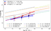 |
Fig. 4. Mass–metallicity relation for galaxies in protoclusters (red) and blank fields (blue), which are based on R3 calibration from C24. The S24 calibration provides similar results, which are listed in the Table B.2 for comparison. The results from other works in the literature are shown with different colors, which are also listed in the Table B.2 for reference. Higher redshift (z > 3) measurements in literature are shown in solid lines, and lower redshift (z ∼ 2 − 3) measurements are shown in dashed lines. |
4.2.1. MZR of the full sample
We perform linear regression on the full sample using Eq. (2). The high sensitivity of NIRCam grism allows us to measure low-mass MZR down to M* ∼ 107 M⊙. We determine the best-fit slope of γ = 0.26 ± 0.01 and an intercept of Z10 = 8.00 ± 0.01. Table B.2 shows our measurements alongside those from the literature. In addition to C24 calibration, we also show the measurements using S24 calibration in Table B.2 for comparison. We can see that the results based on S24 and C24 are consistent with each other.
We find that both the slope and intercept are reasonably consistent with Chakraborty et al. (2025), who conducted the first MZR measurements using the direct Te method. Our best-fit MZR is ∼0.2 dex lower than those observed in CEERS (Nakajima et al. 2023), JADES (Nakajima et al. 2023) and JADES+Primal (Sarkar et al. 2025). A similar offset has been found by Chakraborty et al. (2025), who attributed their discrepancy to the systematic offset between the direct Te method and strong line calibration-based methods. Since we use C24 calibration derived from high-redshift direct Te method, our results are more consistent with Chakraborty et al. (2025). Heintz et al. (2023) and also revealed a low metallicity intercept, who applied S24 calibration, similar to C24 calibration. Aside from the offset in absolute normalization, our observed MZR is consistent with Sarkar et al. (2025), Nakajima et al. (2023), while Curti et al. (2024) reports a flatter slope. Compared with observations at lower redshift, the MZR in the same stellar mass range shows an offset of ∼0.6 dex lower than He et al. (2024) at z ∼ 3. Together with Nakajima et al. (2023), Sarkar et al. (2025), He et al. (2024), for low-mass galaxies (log(M*/M⊙) < 9) the MZR slope at 2 < z < 10 is slightly shallower but not significantly different from that of more massive galaxies (log(M*/M⊙) > 9) at z ∼ 2 − 3 as reported by Sanders et al. (2021) from the MOSDEF survey. While Curti et al. (2024), Li et al. (2023) presented a shallower MZR slope (γ ∼ 0.16 − 0.17 at 2 < z < 9), and Heintz et al. (2023), Chemerynska et al. (2024) show steeper MZR slopes (γ ∼ 0.33 − 0.39 at z > 6).
4.2.2. MZR of field and cluster galaxies
We perform the same linear regression on the field and cluster stacks in our sample. In Fig. 4, we show the MZR measured for field and cluster galaxies using C24 calibration, and in Fig. we show the difference between field and cluster MZRs in comparison with literature studies. We find that galaxies at 5 < z < 7 in overdense environments exhibit a steeper MZR slope than coeval field galaxies, and cluster galaxies are more metal rich than field galaxies, especially at the high-mass end by ∼0.2 − 0.3 dex, indicating enhanced metal-enrichment processes in overdense environments. As a comparison, we also measure the MZR using S24 calibration, and the results are listed in Table B.2. The S24 calibration gives a shallower slope than that using C24 calibration. Thus, we caution that the choice of calibration can affect the observed MZR slope. Despite the systematic difference in different calibrations, the steeper MZR slope of cluster galaxies than field galaxies is confirmed regardless of calibrations. However, we note that, given the typical uncertainties of ≳0.1 dex in metallicity measurements, the observed metal enhancement in overdensities is mild and remains compatible within the measurement errors.
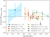 |
Fig. 5. Metallicity offset between galaxies in overdense and field environments. The blue line shows the offset of MZR between cluster and field galaxies, with the shaded region representing a 1σ confidence interval. The single blue diamond shows the offset between the mass-matched cluster and field samples. The measurements in literature (Wang et al. 2022; Kacprzak et al. 2015; Sattari et al. 2021; Kulas et al. 2013; Chartab et al. 2021; Shimakawa et al. 2015; Valentino et al. 2015) are also shown for comparison, each marked in different colors. The error bars represent 1σ uncertainties. |
We also observe that the galaxies in overdense environments are more massive than field galaxies at the same redshift, as in each mass bin, the median stellar mass of cluster galaxies is ∼0.1 − 0.2 dex higher than that of field galaxies. More massive galaxies are intrinsically more metal rich. Although this is expected to be a small effect, to reduce the potential bias of different stellar mass distributions in field and cluster galaxies, we additionally build a mass-matched field sample. We select the field galaxy that is closest in stellar mass to each cluster galaxy and measure the metallicity in the same way discussed above. The measurements in the three mass bins of the cluster and field subsets are listed in Table B.1. We find that, at the same stellar mass, the cluster galaxies are overall more metal rich by ∼0.2 dex compared to their field counterparts, regardless of the choice of S24 or C24 R3 calibrations. The offset of the mass-matched sample is also presented in Fig., and remains consistent with the predicted offsetsin MZR.
5. The fundamental metallicity relation
The FMR relates metallicity, stellar mass and star formation rate (SFR) (e.g., Lara-López et al. 2010; Mannucci et al. 2010; Curti et al. 2020; Sanders et al. 2021; Baker et al. 2023). It is a key scaling relation to understand the physical processes in galaxy evolution. Ellison et al. (2008) show that galaxies with higher SFR systematically exhibit lower metallicity than those with lower SFR at fixed stellar masses. Lara-López et al. (2010) and Mannucci et al. (2010) further show that the scatter in the MZR can be reduced if the SFR is introduced as a secondary parameter with stellar mass, i.e., in terms of the SFR–MZ relation. We apply the parametrization of Andrews & Martini (2013) to describe the SFR–MZ relation by finding the value of α that minimizes the scatter in the metallicity at a fixed μα, defined as
 (3)
(3)
We estimated the SFR by using Hβ luminosity and the Kennicutt (1998) calibration corrected to a Kroupa IMF (as applied by Heintz et al. 2023; Sarkar et al. 2025):
 (4)
(4)
where we converted their calibration using the theoretical ratio fHα/Hβ = 2.86 with case B recombination (Osterbrock 1989). The LHβ is measured from the median stacked spectra. Since Hγ is partially covered in our sample at z > 6.25, we are not able to estimate dust attenuation for the full sample. From our z > 6.25 stacks, the dust attenuation is estimated as  , and we use the same dust attenuation for all the sample galaxies at 5 < z < 7. Considering the large uncertainty of AV, we do not directly correct for dust on LHβ measurements; instead, we use AV = 0.38 as an upper bound for the LHβ error, corresponding to ∼50% flux uncertainty. We add the ∼50% uncertainty into the statistical error in quadrature and propagate it into the SFR estimation.
The estimated SFRs from the median stacks are ![Mathematical equation: $ \left[11.78^{+5.90}_{-0.34},13.54^{+6.79}_{-0.46}, 8.49^{+4.28}_{-0.50}\right]\,M_\odot/\mathrm{yr} $](/articles/aa/full_html/2025/11/aa55372-25/aa55372-25-eq29.gif) , for the [full, field, cluster] samples, respectively. For comparison, we also report the median values of the SED-based SFRs: [9.20,10.14,8.74] M⊙/yr. The SFRs derived from Hβ are generally higher than those estimated from SED fitting, as the Balmer line Hβ reflects the recent star formation, while the SFR derived from SED fitting traces the average star formation rate over a longer timescale.
, for the [full, field, cluster] samples, respectively. For comparison, we also report the median values of the SED-based SFRs: [9.20,10.14,8.74] M⊙/yr. The SFRs derived from Hβ are generally higher than those estimated from SED fitting, as the Balmer line Hβ reflects the recent star formation, while the SFR derived from SED fitting traces the average star formation rate over a longer timescale.
We follow Andrews & Martini (2013) who found that α = 0.66 minimizes the scatter in μα − metallicity plane, for a sample of local low-mass galaxies down to M* = 107.4 M⊙ with direct Te metallicity. They showed that with α = 0.66, the μα − metallicity relation is parameterized as
 (5)
(5)
We note that there are some discrepancies in the literature about the value of α. With SDSS spectra, Curti et al. (2020) and Sanders et al. (2021) suggested α = 0.55 and α = 0.60 respectively, while several studies suggest weaker dependence on SFR, i.e., α ≲ 0.4 (Mannucci et al. 2010; Guo et al. 2016; Henry et al. 2021). The discrepancy in α can be attributed to the sample selections and the choice of the metallicity calibrations. A more detailed discussion about the value of α is beyond the scope of this paper. We use α = 0.66 as is widely used for comparison with recent JWST observations at similar redshifts and stellar mass range (Nakajima et al. 2023; Sarkar et al. 2025).
Previous studies have shown varying results regarding the offset from the local FMR. Curti et al. (2024) and Heintz et al. (2023) reported a significant offset starting from z ∼ 4, while Nakajima et al. (2023) and Sarkar et al. (2025) found no significant deviation at z < 7. The differences in these findings can be attributed to the metallicity calibrations used. Nakajima et al. (2023) and Sarkar et al. (2025) employed calibrations from N22 and C20, which may overestimate the metallicities with respect to C24 by about 0.2 dex, as noted in Chakraborty et al. (2025). Heintz et al. (2023) utilized the S24 calibration, which is based on high-redshift direct Te measurements, making it more consistent with our findings.
Additionally, the choice of α in the FMR formalism affects the results. Comparing the metallicities from references adopting different alpha values could result in a misinterpretation of the predicted metallicities. Heintz et al. (2023) used α = 0.55 from Curti et al. (2020), leading to a metallicity prediction that is ∼0.1 dex higher than predictions using α = 0.66 from Andrews & Martini (2013). Nakajima et al. (2023) also found that using the FMR formalism of Curti et al. (2020) predicts a higher metallicity than using the formalism of Andrews & Martini (2013) at z > 6, and thus get a more negative offset. This difference in α leads to a larger offset observed by Heintz et al. (2023) compared to Sarkar et al. (2025) and Nakajima et al. (2023). While we expect a smaller offset for Heintz et al. (2023) if α = 0.66 is used, there is still a significant offset from the local FMR. Furthermore, Curti et al. (2024) employed a different FMR formalism from Curti et al. (2020), yet this is similar to the parametrization using α = 0.55.
On the other hand, different SFR conversions are applied in different works. Nakajima et al. (2023) assumed Chabrier IMF when converting the Hα or Hβ luminosity to SFR, while Heintz et al. (2023) and Sarkar et al. (2025) assumed the Kroupa IMF. The main FMR results reported by Curti et al. (2020) are based on their SED-derived SFRs. They also provided SFRs converted from Hα luminosities, using a calibration derived from low-metallicity galaxies in Reddy et al. (2022). The Reddy et al. (2022) calibration yields lower SFRs that are about 40% of those obtained using a Kroupa IMF. In contrast, the Kroupa IMF yields SFRs that are higher than those from the Chabrier IMF by ∼6% (Madau & Dickinson 2014), and has a negligible impact on the FMR (Nakajima et al. 2023).
Considering the difference in calibrations and FMR formalism used in different studies, we have recalculated the FMR offsets based on Andrews & Martini (2013) formalism with α = 0.66 for a fair comparison in this work. Since the difference between Kroupa and Chabrier IMFs is negligible, we do not apply any conversion between them, as used by Nakajima et al. (2023), Heintz et al. (2023), Sarkar et al. (2025). However, we convert the Reddy et al. (2022) calibration to a Kroupa IMF for consistency. We note that the recalculated values remain consistent with the original measurements within the quoted uncertainties. Below we list the details of their measurements and our recalculations.
-
Curti et al. (2024) used a revised version of C20 calibration that is refined by a sample of local metal-poor galaxies. We retrieved their measurements from Table B.1 and recalculated the FMR offset using Andrews & Martini (2013) formalism. To account for systematic differences between local and high-redshift Te measurements noted by Chakraborty et al. (2025), we applied a −0.2 dex offset to their metallicities. This offset is based on empirical differences between calibrations (see Fig. 7 in Chakraborty et al. 2025). A more rigorous approach would require recalculating from original line flux measurements, which is beyond our scope. Their SFRs derived from Hα or Hβ fluxes are based on Reddy et al. (2022) calibration, and we converted the SFRs to Kroupa IMF by multiplying a factor of 2.6.
-
Heintz et al. (2023) used S24 calibration, which is calibrated using high-redshift direct Te measurements, and is more consistent with C24 calibration. We do not apply an additional metallicity offset for their measurements. Their offset from FMR is calculated using α = 0.55 from Curti et al. (2020). We retrieved their measurements from their Table 1 and recalculated the offset following Andrews & Martini (2013).
-
Nakajima et al. (2023) used N22 calibration, which is based on a sample of local metal-poor galaxies. They used the same FMR formalism as Andrews & Martini (2013). We added a constant offset of −0.2 dex to their FMR offsets to account for the systematic offset in metallicity calibrations.
-
Sarkar et al. (2025) used C20 calibration. They used the same FMR formalism as Andrews & Martini (2013). We added a constant offset of −0.2 dex to their FMR offsets to account for the systematic offset in metallicity calibrations.
In Fig. 6, we compare the observations of our sample galaxies with the predictions of the local FMR. We find that the full sample galaxies are approximately 0.25 dex lower than the local FMR predictions. Cluster galaxies, however, are more metal rich and slightly offset from the local FMR. From the recalculated offsets in literature studies, we find a similar metal dilution at z > 5 as our observations. Heintz et al. (2023) interprets such an offset by the effective dilution due to pristine gas infall onto the galaxy. In hydrodynamical simulations, Garcia et al. (2024) found a non-negligible evolution in α as a function of redshift, rather than assuming a constant value as we have done with α = 0.66. Garcia et al. (2025) further suggested that the role SFR plays in setting the normalization may change with redshift, and an increasing anti-correlation between MZR and SFR possibly leads to the observed metal deficiency compared with FMR observed at z = 0. The evolving FMR may indicate changing physical processes influencing galaxy metal enrichment, such as gas accretion and feedback.
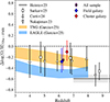 |
Fig. 6. Offsets in metallicity between observations and the predictions of the local FMR with α = 0.66 (Andrews & Martini 2013). The orange and blue shadows represent the predictions in TNG and EAGLE simulation (Garcia et al. 2025). The offsets reported by Curti et al. (2024), Heintz et al. (2023) used a different FMR formalism, and we recalculated the offsets using Andrews & Martini (2013) formalism. For Nakajima et al. (2023), Sarkar et al. (2025), we added a constant offset of −0.2 dex to their FMR offsets to account for the systematic offset in metallicity calibrations used in their studies. |
6. Simple analytical model of chemical evolution
6.1. Model description
To help understand the physical origin of star formation and metal enrichment, many analytical models of galaxy chemical evolution have been proposed (Edmunds 1990; Edmunds & Greenhow 1995; Köppen & Edmunds 1999; Finlator & Davé 2008; Erb 2008; Davé et al. 2012; Dayal et al. 2013; Lilly et al. 2013; Peng & Maiolino 2014; Guo et al. 2016; Wang & Lilly 2021; Toyouchi et al. 2025). Several studies have used a “closed box” model or “leaky box” model to explain the evolution of MZR (Ma et al. 2016; Langan et al. 2020), which is a modified version of “closed box” model, while using an effective yield (peff) instead of the yield (p) to account for flows of metals through inflow and outflow. The yield p is defined as the mass in metals returned to the ISM relative to the mass in stars formed:  (Pagel & Patchett 1975). In the “leaky box” model, the ISM metallicity is simply a function of effective yield and gas fraction:
 (6)
(6)
where fgas is defined as the mass fraction of gas to the total mass of gas and stellar components. When peff = p, the system is a “closed box” and the metallicity only depends on the consumption of the initial gas reservoir and metal production within the system. When peff < p, the system is “leaky” and the metals are lost by metal-enriched outflow. However, the detailed pathways of those metal flows are not explicitly modeled.
To capture more details, here we model the galaxy ISM as an open system with gas inflow and outflow, and consumption of gas by star formation (also known as the “bathtub” model) (See Pagel 2009; Bovy 2026, for helpful reviews). Following Erb (2008), with the conservation of gas mass, we have the relation
 (7)
(7)
where Ṁin and Ṁout are the mass flow rate of gas inflow and outflow, and μ is the fraction of mass that is locked in long-lived stars and remnants, i.e., (1 − μ) represents the efficiency of gas return from SNe.
With the conservation of metal mass, we have
 (8)
(8)
where Zin is the metallicity of gas inflow, Zout is the metallicity of gas outflow, and ZSFR is the metallicity of the gas forming stars, and y is the metal yield. The first term on the right-hand side is the metal mass flow rate from the gas inflow. The second term represents the metal enrichment from metals produced from star formation. We note that we used adifferent definition of yield, y, (e.g., applied by Erb 2008) in order to distinguish from p in Eq. (6). We defined y as the mass in metals returned to the ISM relative to the mass of hydrogen consumed by star formation instead of the total stellar mass formed:  (Searle & Sargent 1972). With this definition, (1 − ZSFR) represents the fraction of hydrogen that contributes to chemical enrichment, given that the metals incorporated into star formation are not further available for subsequent metal production. Other works using the definition p do not include the (1 − ZSFR) term (e.g., Peng & Maiolino 2014). Since the metal content is low relative to hydrogen, these two different definitions do not result in any significant differences in reasonably low metallicity ranges. The third term is the metal mass loss from gas outflow, and the fourth term is the metal consumption when ISM gas, together with metals therein, collapses into stars.
For simplicity, here we assume that μ = 1, i.e., gas returned to the ISM is negligible. We assume that the metallicity of gas forming stars is the same as ISM gas: ZISM = ZSFR, and the inflowing gas is metal-free: Zin = 0. The outflow metallicity is assumed to be the same as the ISM metallicity. We further assume a steady-state approximation: the gas and metal masses are in the state of dynamic equilibrium:  (also see Davé et al. 2012). For low metallicity galaxies with ZSFR ≪ 1 such that 1 − ZSFR ≈ 1, Eq. (8) indicates the ISM metallicity:
 (9)
(9)
The mass outflow rate is related to the SFR and mass loading as
 (10)
(10)
where η is the mass loading factor, defined as the amount of gas ejected per unit mass of star formation, and λ > 0 allows the outflow rate to non-linearly correlate with SFR. For instance, simulations suggest that if stars form in clusters with a higher SFR, the successive feedback from supernovae (SNe) in clusters can create superbubbles large enough to break out of the galactic disk, enhancing the outflow efficiency (Orr et al. 2022). Wind models show that the mass loading factor is related to halo masses:  for momentum-driven wind (kinetic feedback) and
  for energy-driven wind (mechanical feedback), derived either via momentum or energy conservation (Davé et al. 2012). The halo mass can be estimated with the Stellar-to-Halo mass relation: Mh = ℱ(M*) (e.g., Moster et al. 2010; Behroozi et al. 2013; Shuntov et al. 2022, 2025). We have
 (11)
(11)
where η0 is the mass loading factor at a reference halo mass M0, and β characterizes the mass dependence of the mass loading factor, i.e., β = 1/3 for momentum-driven wind and β = 2/3 for energy-driven wind. Different β values are also adopted in other semi-analytical models to treat SNe feedback (Cole et al. 1994; Guo et al. 2011). We do not include AGN feedback in our model, as it is not the primary focus for young star-forming galaxies. Replacing Ṁout in Eq. (9), we have
 (12)
(12)
The above solution relies on a steady-state approximation. However, if the galaxy is accumulating gas more rapidly than its depletion, i.e., Ṁgas > 0, the galaxies live in a non-equilibrium state (e.g., Peng & Maiolino 2014). We could perturb the above steady-state solution by adding an instant gas dilutionterm:
 (13)
(13)
where τacc is the gas accretion timescale defined as τacc = Mgas/Ṁin, and τdepl is the gas depletion timescale: τdepl = Mgas/SFR. This describes the amount of extra gas accreted onto the galaxy in an episode of gas depletion after prior gas accretion. If τdepl > τacc, gas accretion is faster than gas depletion, and the ISM metallicity is more diluted than its steady-state solution. We defined ϵacc as the efficiency relating the SFR to the gas accretion rate:
 (14)
(14)
which describes the fraction of accreted gas that is converted to stars (e.g., Davé et al. 2012.) Similarly, we also define the star formation efficiency3 as the ratio of the SFR to the total gas mass:
 (15)
(15)
The Kennicutt–Schmidt law (KS law, Schmidt 1959; Kennicutt 1989) describes the relation between surface densities of star formation and gas mass:
 (16)
(16)
Kennicutt (1998) suggested that n ≈ 1.4 for local star-forming galaxies. The total SFR is the integral of the surface density of star formation over the surface area (s) of the galaxy:
 (17)
(17)
With a crude approximation that the gas surface density is a constant across the galaxy and does not evolve with time, even though the gas mass changes, the SFR is linearly correlated with the gas mass as one galaxy evolves:
 (18)
(18)
The SFR no longer explicitly depends on n, naturally following from Eq. (15). In this sense, the galaxy is accumulating mass with growing size/volume, while keeping the same gas density, although this might not hold as the gravitational potential changes. Here, the ϵSF implicitly describes the KS law, with a larger ϵSF indicating a higher gas density, which produces a higher SFR. In our assumption, the ϵSF is a constant through the evolution of a single galaxy, but the value can vary for different galaxies with different gas densities to keep the KS law.
The above relations naturally suggest τacc/τdepl = ϵacc, so the observed metallicity from Eq. (13) is then
 (19)
(19)
and in log scale, it is
 (20)
(20)
If the outflow rate is dominant, i.e., ηSFRλ − 1 ≫ 1, the observed metallicity is then approximated as
 (21)
(21)
This solution relates the observed metallicity to the steady-state metallicity, the SFR, and the stellar mass. With a fixed stellar mass and gas mass, the mass loading term is a constant. The observed metallicity is then a simple linear function of logSFR:
 (22)
(22)
This is in the same form as the formalism of FMR in observations (e.g., Eqs. (3), (5)).
In cases where the outflow is small, i.e., ηSFRλ − 1 ≪ 1, the observed metallicity is then approximated as
 (23)
(23)
This relation is less linear, but it also predicts the decreasing metallicity with increasing SFR.
We note that the observed metallicity actually varies with the age of the galaxy we observe. A more strict solution can be derived by solving the differential equations using Eqs. (7) and (8) and inferring the metallicity evolution with galaxy ages. The strict solution also suggests that all galaxies will eventually reach their steady-state metallicities at sufficiently large age, no matter how much the gas accretion rate is. We also note that ϵacc is actually not a constant, and varies with SFR as galaxies evolve. The dilution by the factor of ϵacc is a simple proxy for the delay of metal enrichment due to intense gas accretion at the beginning of galaxy formation. As a galaxy evolves, the gas reservoir builds up and reaches equilibrium, the star formation rate peaks with a higher ϵacc, and the dilution effect is reduced.
To better illustrate such time evolution during a non-equilibrium state, we further discuss the results of numerical solutions in the context of MZR and FMR evolution in Sections 6.2 and 6.3.
6.2. Numerical solutions of model equations
Mannucci et al. (2010) suggested that the FMR originates when galaxies are observed in a transient phase where the dilution effect from gas infall dominates over the metallicity enrichment from newly formed stars; thus, understanding the time evolution of the mass assembly and metal enrichment can be important. We show that this can be revealed from the solutions of Eqs. (7) and (8). We have constructed different sets of models exploring different parameter spaces. In all models with outflow, we have assumed feedback is linearly correlated with SFR, i.e., λ = 1. We use the same initial conditions for all the models with inflow: a pre-existing gas reservoir Mgas, 0 = 106 M⊙, with few stars M*, 0 = 101 M⊙ and metal-free ZISM, 0 = 0. For models without inflow, we assigned a different pre-existing gas mass, 105.0 − 1010.0 M⊙, for different galaxies. Following Erb (2008), we used the stellar yield y = 0.019 = 1.5 Z⊙ for all the models, where Z⊙ = 0.0126 is the solar metallicity (Asplund et al. 2004, 2009). In the steady-state solution, we have assumed μ = 1 as no gas recycling in Eq. (7). However, the gas returned from massive stars can be non-negligible for a longer duration of star formation; for example, the fraction of mass returned from stars approaches 40% of the total stellar mass formed for a Chabrier IMF in a few gigayears (Erb 2008). For a top-heavy IMF, the fraction of mass returned can be higher. While the time-varying return fraction can be non-trivial, we approximate a time-invariant return fraction 40% with μ = 0.6 for simplicity. This implies the instantaneous recycling approximation, which is generally appropriate for metal yields from short-timescale massive-star evolution, particularly oxygen (Pagel 2009). We varied other parameters to explore the effects of different feedback strengths and star formation efficiencies in the following five model sets.
-
Model 1: Incorporating inflow but no outflow, with a varying star formation efficiency ϵSF = [0.02, 0.05, 0.1]×106 Myr−1. Observations of giant molecular clouds in the Milky Way suggest a star formation efficiency per free-fall time in the range of 0.002–0.2 (Murray 2011). Our adopted values are therefore reasonable, given that the free-fall time for galaxies at z > 5 could be on the order of ∼1 Myr (Dekel et al. 2017). We fix η0 = 0 so that no gas is removed from the galaxy. We use the constant gas accretion rate between 105.5 and 109.0 M⊙ Myr−1 for different galaxies.
-
Model 2: Incorporating outflow but no inflow, varying star formation efficiency ϵSF = [0.02, 0.05, 0.1]×106 Myr−1. We fixed Ṁin = 0 so that no gas is accreted from the intergalactic medium, and the galaxy only consumes the gas pre-existing in the reservoir, set as 105.0 − 1010.0 M⊙ for different galaxies.
-
Model 3: Incorporating both inflow and outflow, varying mass loading factor η0 = [0.5, 1, 2]. We assume the same normalization halo mass M0 = 1010 M⊙ in Eq. (11). We applied the stellar-to-halo mass relation at z = 5 from Shuntov et al. (2022) to convert the stellar mass to the halo mass, which constrains the outflow rate in Eq. (11). We use the constant gas accretion rate between 105.5 and 109.0 M⊙ Myr−1 for different galaxies.
-
Model 4: Incorporating both inflow and outflow, varying outflow mode β = [0, 1/3, 2/3, 1]. Specifically, β = 0 corresponds to the constant wind model (η = η0), β = 1/3 corresponds to the momentum-driven wind model, and β = 2/3 corresponds to the energy-driven wind model. In addition, β = 1 corresponds to a stronger wind model, where the outflow rate scales more significantly with halo mass. The physical mechanisms of SNe feedback remain less clear when assuming β = 1. However, similar values are also adopted in semi-analytical models to reproduce the observed luminosity or stellar mass functions (e.g., Guo et al. 2011). Other parameters in this set are the same as in Model 3. We use the constant gas accretion rate between 105.5 − 109.0 M⊙ Myr−1 for different galaxies.
-
Model 5: Incorporating both inflow and outflow, with parameters fixed to match the observations at 5 < z < 7. We used ϵSF = 0.02 × 10⁶ Myr−1, η0 = 5 and β = 2/3.
We obtained the solutions of the above models by integrating the differential equations using fourth-order Runge-Kutta method. The results contain arrays of time and other variables at each time step. To explore the FMR evolution, we match the SFR and stellar mass for different galaxies. The results are shown in Fig. 7. Similarly, to obtain the time evolution of MZR, we defined the tobs of a galaxy as the time elapsed since the onset of gas accretion and star formation, and we pick up galaxies with different tobs. Using model 5, we show the predicted MZRs with different tobs in Fig. 8. In Fig. 7, we see that the high-mass galaxies show a flatter Z − SFR relation than low-mass galaxies, and at fixed stellar masses, a higher star formation rate leads to lower metallicities, which are qualitatively consistent with the observations (e.g., Andrews & Martini 2013; Curti et al. 2020). We discuss the implications of the results in the following Section 6.3.
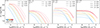 |
Fig. 7. Predicted Z − SFR relations for different model configurations. First panel: model 1, incorporating inflow but no outflow, with ϵSF as the varying parameter. Second panel: model 2, incorporating outflow but no inflow, with ϵSF as the varying parameter. Third panel: model 3, incorporating both inflow and outflow, with η as the varying parameter. Fourth panel: model 4, incorporating both inflow and outflow, with β as the varying parameter. In all panels, the lines are color-coded by stellar mass, while different line styles indicate variations in model parameters. |
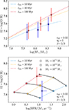 |
Fig. 8. Top: predicted MZR for galaxies with different tobs. The dashed lines are MZRs color-coded by tobs. This model assumes ϵSF = 0.02, η0 = 5, and an energy-driven wind β = 2/3. The diamond points are our observations, the same as in Fig. 4. Bottom: Predicted SFR−Z relation for galaxies is shown for different stellar masses and tobs. The dashed lines, color-coded by tobs, connect galaxies with the same observational time, while the solid black lines link galaxies of equal stellar mass. Different stellar masses are represented by different symbols. The red and blue diamond points are our observations in cluster and field environments. The asymmetric errors on SFR are due to uncertainties in dust correction. |
6.3. Model implications of FMR evolution
For the case where FMR is independent of redshift, such a non-evolving FMR implies that the metallicity is a fixed function of SFR, at fixed stellar masses. Under steady-state condition, this indicates that Eq. (21) is not changing with redshift, which requires that
 (24)
(24)
A constant λ indicates that the outflow gas has the same response to star-forming feedback. And a constant yϵacc/η requires that the metal yield, gas dilution, enrichment, and mass loading factor are either constant or maintain the same balance across cosmic time.
Before z ∼ 3, observations show that the FMR is nearly independent of redshift (Mannucci et al. 2010; Henry et al. 2021). However, literature studies suggest that the FMR starts to evolve at z ≳ 3 (Mannucci et al. 2010; Curti et al. 2024). Møller et al. (2013) suggests a transition phase of primordial gas infall at z ∼ 2.6, which may be relevant for such evolution.
Although the origin and evolution of the FMR remain unclear, it is instructive to explore its possible consequences within the framework of our simple model. In the following sections, we consider variations in gas accretion, star formation efficiency, feedback processes, and potential environmental effects.
6.3.1. Gas accretion and star formation efficiency
Equation (13) indicates that a lower metallicity is related to a lower efficiency ϵSF, which happens when the gas accretion rate is high, and the metal enrichment of ISM is delayed. In this case, the gas reservoirs of galaxies at z > 5 are in a more non-equilibrium state, with high gas fraction and low metallicity. This is consistent with observations of abundant gas reservoirs at high redshifts (Heintz et al. 2022). Dekel et al. (2017) proposed the feedback-free starburst scenario where cold gas accretion onto halos at z > 5 occurs without being heated by virial shocks. In this scenario, star formation proceeds efficiently due to short free-fall times in star-forming clouds compared to feedback timescales from SNe. This high local star formation efficiency is compatible with our observed metal dilution effect because the overall ISM metallicity remains dominated by the inflowing cold gas streams, with newly produced metals not fully mixing with these streams (Dekel et al. 2017; Li et al. 2024b). Thus, the observed lower metallicity results from enhanced metal dilution due to intense gas accretion at z > 5.
In the first panel of Fig. 7, we show the predicted FMR with model 1, where the galaxies are fed with continuous inflow with varying star formation efficiency ϵSF. We observe that the Z − SFR relation is sensitive to ϵSF, with a lower ϵSF leading to a lower metallicity for a given SFR and stellar mass. This aligns with the prediction of Eq. (13), which indicates that a lower ϵSF results in a reduced SFR, leading to a lower ϵacc and a stronger dilution effect. In the second panel of Fig. 7, we show the predictions from model 2, where no inflows are available, but the galaxies can consume the gas pre-existing in the gas reservoir. We find a similar trend of FMR evolution with ϵSF. The high rate of continuous inflows acts similarly to the pre-existing pristine gas reservoirs, as in both cases, the galaxies are in a non-equilibrium state due to abundant gas supply at the beginning of star formation. But model 2 is less realistic: The assumption of massive initial gas reservoirs without prior star formation is unlikely, as dark matter halos with masses Mh ≳ 108 M⊙ already start to cool and collapse to boost star formation (Klessen & Glover 2023). Nevertheless, both models highlight the effects of the delay of metal enrichment due to gas dilution in shaping the FMR evolution, and a lower ϵSF leads to extra metal deficiency.
6.3.2. Feedback
The feedback strength impacts the metal retention in galaxies. Eq. (21) indicates that the observed metallicity both depends on mass loading factor η and the outflow response of star formation λ. From Eq. (21), an enhanced λ leads to a steeper slope of FMR, which leads to a lower metallicity for a given SFR and stellar mass. The mass loading factor η sets the normalization of FMR. A higher η leads to an enhanced metal loss and lowers the metallicity intercept of FMR.
In the third and fourth panels of Fig. 7, we show the predicted FMR with model 3 and model 4, with galaxies fed by continuous inflow and varying mass loading factor η and outflow mode β. The FMR is sensitive to both parameters. Higher η produces lower metallicity at given SFR and stellar mass, consistent with Eq. (21), where higher η causes stronger metal loss. For model 3, metallicity plateaus at low SFRs indicate equilibrium states where metal production balances metal loss. These plateaus are higher in metallicity with lower η due to less efficient winds. Model 4 shows similar behavior, with plateaus at low SFRs where β has maximum impact. Varying β changes the dependence on halo mass and modifies the outflow gas content.
In observations, however, Zhang et al. (2024), Xu et al. (2025b) suggest less efficient outflows at z > 6 with low wind velocities. Such kind of low-velocity winds are likely producing fountain-type outflows, where the ejected gas and metals cannot escape from the gravitational potential well and eventually reaccrete onto the galaxy. The reaccretion of pre-enriched streams aids galaxies in retaining their metals (Zhang et al. 2023). On the other hand, the stellar yield y also affects the normalization of FMR. An evolving IMF can lead to different stellar yields (van Dokkum 2008). For instance, a top-heavy IMF results in a higher total metal yield compared to a standard or bottom-heavy IMF due to increased proportion of massive stars (Vincenzo et al. 2016). From recent JWST observations, Zou et al. (2024), Hutter et al. (2025) suggest a top-heavy IMF at z > 6 using chemical abundance patterns and UV luminosity functions. While we expect a higher metal yield with such a top-heavy IMF, those constraints on feedback cannot solely explain the metal deficiency at z > 5 in our observations. Thus, the models and observations suggest that feedback is not the dominant process driving metal deficiency at z > 5.
6.3.3. Environmental effects
Equation (13) indicates that there is a delay of metal enrichment compared to the steady-state solution due to faster gas accretion than gas depletion. Helton et al. (2024a) found that cluster galaxies at z ∼ 5 have earlier star formation, by comparing SFR at different epochs of SFH. They found that galaxies in an overdensity show both a higher SFR0 − 100 Myr and SFR30 − 100 Myr/SFR0 − 30 Myr ratio than their mass-matched field counterparts. They indicate that overdensity galaxies have already undergone significant star formation at 30 − 100 Myr before observation, while the major star formation for field galaxies just started in the last 30 Myr. Estimated from the SED fitting, we find that the stellar masses observed in the overdensities are more massive by ∼0.1 dex than field galaxies. In contrast, their median [O III] and Hβ luminosities are ∼0.1 dex lower than those of the field. Since Hβ emission traces the instantaneous SFR, this suggests that field galaxies are forming stars more actively, consistent with the scenario of enhanced recent star formation in the field. In addition, weaker nebular emissions like [O III] in overdensities also indicate more evolved systems. However, because the [O III] and Hβ lines are sensitive to dust, and Li et al. (2025) suggested that galaxies are more dusty in the overdensities, we caution possible uncertainties in [O III] and Hβ fluxes and derived SFRs for the twosamples.
Supposing the cluster galaxies are more evolved, they should be closer to equilibrium with a higher observed metallicity close to the steady-state solution in our models. We further investigate such effects from model 5. Using the model output grids, we select galaxies at different times since formation tobs = [10, 30, 100] Myr, which can alternatively be interpreted as the “age” of the galaxy. In the top panel of Fig. 8, we show the predicted MZR for galaxies with different tobs. We find that galaxies with longer durations of star formation have higher metallicities. The galaxies observed at tobs = 10 Myr show a flatter MZR slope, while those observed at tobs = 100 Myr show a steeper slope with ∼0.2 dex higher metallicities. The steeper slope can be predicted by Eq. (12). We have adopted λ = 1 in the model, and now we approximate η ≫ 1. In a steady-state solution, the slope of MZR can be estimated by
 (25)
(25)
where log(ℱ)′ is the derivative of Halo-to-Stellar mass function in log space. For halos at z ∼ 5, masses lower than Mh = 1012 M⊙, log(ℱ)′ can be approximated as a constant ≈0.6 (Shuntov et al. 2022). As a result, the MZR slope4 is estimated as ≈0.6β for low-mass galaxies at z ∼ 5. For energy-driven wind used in our model, we expect a slope of ∼0.4 when reaching steady-state conditions. For galaxies with longer time to evolve, i.e., the solutions with tobs = 100 Myr, they are closer to equilibrium, and the observed MZR slope is close to the steady-state approximation. This indicates that the MZR can vary with time during non-equilibrium phases for galaxies with ongoing gas accretion. In addition, our model suggests energy-driven wind with mechanical feedback to produce the observed MZR in the non-equilibrium phase. A momentum-driven wind with β = 1/3 is also possible, but it requires the steady-state condition for all the galaxies to match the predicted slope γ ≈ 0.6 × 1/3 = 0.2.
In the bottom panel of Fig. 8, we show the predictions of the Z-SFR relation from the same output of model 5. We see that at the same time of observation, more massive galaxies have higher metallicities, which is expected by MZR predictions. We also find that FMR evolves with time; the contours denoting the observation time are moving upward as time increases. This indicates that the FMR evolves with time, and the different stages of SFH can also be a driver of FMR. We also compare our observations in the bottom panel of Fig. 8. We find that the Z − SFR relations for cluster and field samples are not moving along the predicted contour of stellar mass at fixed observation time, while they cross the contours of both stellar masses and observation time. The model predictions are consistent with the case that cluster galaxies are more massive and older than field galaxies. Thus, the model suggests a later evolution phase for cluster galaxies and a younger stage for field galaxies. If cluster galaxies have earlier star formation, we expect them to be more metal rich than field galaxies on the FMR diagram from our model predictions. Our observation thus suggests that cluster galaxies have an earlier onset of star formation within a non-equilibrium scenario, consistent with the finding of Helton et al. (2024a).
7. Discussion
7.1. Comparison with hydrodynamical simulations
We recognize that our analytical model is oversimplified. Any small-scale processes are not modeled, such as gas dynamics including rotation, turbulence, diffusion, and advection (e.g., Sharda et al. 2021). The ISM gas-phase structures are not considered, and the more detailed processes in feedback, such as heating and cooling, are not included either (see, e.g., Collacchioni et al. 2018). And the star formation efficiency can be modulated by feedback, which is not considered in our model. We have also assumed that the inflowing gas is metal-free Zin = 0. However, this may not always hold true in realistic environments. The IGM can be enriched by earlier generations of galaxies, and inflowing gas may also contain recycled material from the circumgalactic material (CGM) that has been ejected and subsequently reaccreted (Beckett et al. 2024), especially if the outflows are not powerful enough to escape the galaxy’s gravitational potential. Simulations and observations suggest that the CGM of high-redshift galaxies is often enriched, and the metallicity of inflows may depend on cosmic time, halo mass, and the surrounding galaxy environment (Anglés-Alcázar et al. 2017). As such, the inflow metallicity may vary with environment, star formation rate, and dynamical timescales, and could potentially correlate with Zout and Ṁout, though this relation is non-trivial in practice.
Thus, comparing observations with numerical simulations helps understand the physical processes. Various hydrodynamical simulations have studied metal enrichment in galaxies, including EAGLE (De Rossi et al. 2017), FIRE (Ma et al. 2016), FIREBOX (Bassini et al. 2024), FIRE-2 (Marszewski et al. 2024), ILLUSTRISTNG (Torrey et al. 2019), FIRSTLIGHT (Langan et al. 2020), ASTRAEUS (Ucci et al. 2023), SERRA (Pallottini et al. 2025), and FLARES (Lovell et al. 2021). In Fig. 9, we compare our observations with these simulations. Our full sample’s MZR is generally consistent with FIRE, FIRE-2, and ASTRAEUS simulations, while FIRSTLIGHT and ILLUSTRISTNG predict higher metallicity normalizations. However, metallicity definitions vary between simulations. For example, Marszewski et al. (2024) defines gas-phase metallicity as the mass-weighted mean metallicity of gas particles within 0.2 virial radius, while Ma et al. (2016) used 0.1 virial radius and required gas temperatures below 104 K. Different metal yield prescriptions also affect the absolute metals produced in simulations. For instance, Langan et al. (2020) used yields from Woosley & Weaver (1995) and defined solar metallicity as 12 + log(O/H) = 8.9, higher than in other studies like Torrey et al. (2019). Therefore, the MZR slope is more informative than its absolute normalization, as it traces relative metal enrichment across stellar masses, reflecting the competition between star formation, inflows, and outflows. Fig. 9 shows that ASTRAEUS and ILLUSTRISTNG simulations best match our observed slopes. FIRE and FIRE-2 predict steeper slopes but remain within 1σ errors, while FIRSTLIGHT predicts a steeper slope closer to our observations in overdense environments.
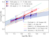 |
Fig. 9. Observed MZR compared with hydrodynamical simulations. The symbols for our observations are the same as in Fig. 4. The results at similar redshifts from different suites of hydrodynamical simulations are denoted by different colors, including FIRSTLIGHT (Langan et al. 2020), FIRE (Ma et al. 2016), FIRE-2 (Marszewski et al. 2024), ILLUSTRISTNG (Torrey et al. 2019), and ASTRAEUS (Ucci et al. 2023). |
Ibrahim & Kobayashi (2024) investigated the impact of different feedback mechanisms on MZR using hydrodynamical simulations based on GADGET-3 code. They find that mechanical feedback best reproduces observations up to redshift z ∼ 3. Our analytical model also suggests the presence of mechanical feedback at z ≈ 5–7, although it alone is insufficient to reproduce the observations. From FIREBOX simulation, Bassini et al. (2024) suggest that the evolution of MZR at z ≲ 3.5 is driven by inflow metallicity, outflow metallicity, and mass loading factor, rather than gas fraction (e.g., De Rossi et al. 2017; Torrey et al. 2019). On the other side, Marszewski et al. (2024) found a weak evolution of MZR at z ≳ 5 in FIRE-2 simulations with a non-evolving slope γ = 0.37. They find that the gas fractions are mass-dependent and vary substantially with redshift, which indicates gas fractions alone cannot explain weakly evolving MZR, and inflows and outflows must be taken into account. Anglés-Alcázar et al. (2017) suggest that recycled gas also plays a crucial role in shaping galaxy metallicities across different stellar masses, with low-mass galaxies being more likely to accrete pre-enriched gas, while high-mass galaxies primarily accrete pristine gas. Langan et al. (2020), Ma et al. (2016) found that a “leaky box” model can reproduce the MZR evolution at z ≳ 3.5 in simulations, but it requires an effective yield (yeff) an order of magnitude smaller than intrinsic stellar yield y, highlighting the non-negligible impact of inflows and outflows.
Wang et al. (2023b) have investigated the environmental effect on MZR at z ≲ 2 using EAGLE simulation. They found that both the suppression of gas accretion and the ram pressure stripping contribute to the environmental dependence of satellite galaxies at z ∼ 2. The ram pressure strips the ISM gas as satellite galaxies move across the clusters and come into contact with the hot ICM. It leads to starvation of the satellite galaxies, preventing further gas accretion, and the galaxies become more metal rich. Additionally, they observed that central galaxies in protoclusters at z ∼ 2 tend to reside in more massive halos, accrete more gas through cold-mode accretion, and consequently exhibit lower metallicities.
On the other hand, directly comparing our observations in overdense environments with simulations at z > 5 remains highly challenging. Simulating low-mass galaxies at high redshifts requires high resolution of particles (e.g., baryon particle mass < 105 M⊙), while simulating the large scale structures requires a large simulation box (e.g., ∼1 Gpc scale). At present, hydrodynamical simulations capable of meeting the requirements of both large and small scales have yet to be fully developed. For example, recent TNG-CLUSTER simulations have provided simulated galaxies in massive clusters within a ∼1 Gpc3 volume (Nelson et al. 2024), but their baryon particle of ∼107 M⊙ is too massive to resolve low-mass galaxies.
7.2. Implication of environmental effect on MZR
Our analytical models demonstrate that the differences in MZR and FMR between field and cluster galaxies can be explained by delayed metal enrichment, primarily caused by the dilution effect of gas accretion. In overdense environments, earlier star formation and rapid metal enrichment may be enhanced compared to blank fields.
Environmental effects on galaxy metallicities remain debated in the literature. For example, Wang et al. (2022), Li et al. (2022) found a flatter MZR in a massive protocluster at z = 2.24, indicating that massive protocluster galaxies are more metal-poor than their field counterparts. Similarly, Calabrò et al. (2022) observed more metal-poor galaxies located in denser environments compared to those of similar masses in underdense regions. In support of these findings, EAGLE simulations (Wang et al. 2023b) suggest that low-metallicity gas accretion dilutes the metallicities of massive central galaxies, while gas stripping suppresses cold gas accretion in lower-mass satellites-consistent with the observations in Wang et al. (2022).
Ram pressure stripping is a possible, but uncertain, mechanism at z > 5. At z ∼ 2, metal enhancement in protocluster galaxies has been observed by Pérez-Martínez et al. (2023), Shimakawa et al. (2015), who attribute it to more efficient gas recycling or gas stripping (Kulas et al. 2013). While gas stripping could contribute to metal enhancement in protocluster galaxies, the early stage of protocluster formation implies that their halos are not yet virialized, and the ICM is expected to remain relatively cool. Whether the ICM is sufficiently hot and dense to support ram pressure stripping and suppress gas accretion remains unclear (Jáchym et al. 2007; Boselli et al. 2014; van de Voort et al. 2017). The evidence for ram pressure stripping at the highest redshifts is currently up to z = 2.51 (Xu et al. 2025a), leaving its effectiveness at z > 5 largely unexplored.
Strangulation might still play a role in z > 5 protoclusters. The gravitational potential of the protocluster halo could induce tidal stripping of ISM gas, inhibiting further gas inflow and leading to enhanced metallicity (Peng et al. 2015). This scenario is consistent with our observations: in our non-equilibrium framework, galaxies that evolve closer to chemical equilibrium exhibit higher metallicities, reflecting a later evolutionary phase. If gas accretion is suppressed via tidal effects in overdense environments, equilibrium between metal production and dilution can be achieved earlier. However, we note that while this explanation aligns with our observations, direct observational evidence of strangulation remains lacking.
Whether gas accretion or gas stripping dominates in overdense environments may also be mass-dependent. Studies at z ∼ 2 suggest that massive galaxies are more affected by gas accretion, while low-mass galaxies are more sensitive to gas stripping (Wang et al. 2023b), although the stellar mass threshold between the two mechanisms remains uncertain. As shown in Fig., metallicity deviations between overdense and field environments across different studies are different, even when their galaxy samples fall within the same mass and redshift range. One explanation is that environmental effects depend on the nature of the overdensity itself-redshift, halo mass, and virialization state may all relate to the environmental effects. For example, early-stage protoclusters at high redshift may have different effects than virialized clusters at lower redshift: the effect of cold gas accretion may be active in early protoclusters, while the gas supply could be suppressed by the hot halo of virialized clusters.
Chiang et al. (2017) outlined three major phases of cluster evolution. In the early phase (z ≳ 5), protoclusters begin forming in the densest regions through an “inside-out” process, with accelerated central star formation. The intermediate phase (z ∼ 5 − 1.5) involves rapid stellar mass assembly and structural growth, while the late phase (z < 1.5) is marked by satellite accretion and gradual suppression of star formation. Our protocluster candidates at z > 5 are likely in the early phase, undergoing active mass assembly with significant variation in their properties. As noted by Pérez-Martínez et al. (2023), even protoclusters at the same redshift may be at different evolutionary stages, leading to diverse environmental effects. Thus, combining all overdensities into a single subsample may average meaningful variations (Morishita et al. 2025b). Case-by-case investigations of individual protoclusters at z > 5 are subject to future study (Li et al., in prep.).
In short, the environmental effects on the MZR are complex. The enhanced metallicities we observe in z > 5 protoclusters are consistent with accelerated star formation in overdense regions (Helton et al. 2024a; Morishita et al. 2025a) and align with our non-equilibrium chemical evolution models. Strangulation due to tidal effects is also a plausible contributor to faster metal enrichment (Peng et al. 2015). Ram pressure stripping could enhance metallicities, but its role remains uncertain given the likely cooler ICM conditions in early protoclusters at z > 5.
7.3. Caveats in MZR measurements
Given the uncertain systematics associated with different metallicity measurements (e.g., strong line calibrations and Te method) and different line indicators (e.g., R3, Ne3O2, N2Hα) used across various studies, the origin of the discrepancy in MZR slopes remains elusive. In this study, we only used the R3 line ratio to derive the metallicity and assumed the low-metallicity solution of metallicity. There are potentially higher metallicity galaxies calculated as low metallicity ones. In addition, we are using stacked spectra to derive the MZR. The intrinsic scatter of the MZR relation cannot be estimated from the median measurements. In addition, we are only estimating the median from the stacked samples, so that the actual range of metallicities is still not constrained. While the stacked measurements are representative of the median properties, and the observed trends from stacks appear real, uncertainties in both the metallicity calibrations and the measurements imply that the differences remain compatible within the errors. Calibrations such as R3 could be affected if galaxies with extreme star formation episodes dominate the stack, especially since our sample is selected by [O III] emission and may be biased toward stronger emission-line galaxies compared to the NIRSpec sample used for calibrating the R3 relation.
Furthermore, the measurements of stellar masses also introduce systematic uncertainties in MZR. Whitler et al. (2023) shows that the assumption of SFH significantly influences the determination of stellar masses during SED fitting. Since young stars dominate the observed rest-UV and optical SED, they can outshine any older stellar populations present in the galaxy. As a result, the choice of the SFH model significantly impacts the derived properties, particularly the early SFH, stellar age, and total stellar mass of the system. Different literature studies have different assumptions of SFH, and this can introduce systematic uncertainties in stellar mass measurements and thus the derived MZR. Nakajima et al. (2023) and Heintz et al. (2023) assumed a non-parametric SFH. Chakraborty et al. (2025) and Sarkar et al. (2025) assumed a constant SFH. Curti et al. (2024) assumed a delayed-exponential SFH.
However, as Curti et al. (2024) incorporates samples from Nakajima et al. (2023), they mix galaxies analyzed with different SFH assumptions. Heintz et al. (2023) notes that non-parametric SFH typically increases stellar mass estimates by 0.5 − 1.0 dex compared to parametric approaches (constant or delayed-exponential SFH). This mixing of “high mass” galaxies from non-parametric SFH with “low-mass” galaxies from parametric SFH introduces systematic uncertainties in the MZR. For a sample with similar metallicities, higher stellar mass estimates will shift points rightward on the MZR plot, potentially flattening the slope and possibly explaining the flatter MZR in Curti et al. (2024). While using consistent SFH assumptions reduces impact on the slope, it still affects normalization (e.g., a ∼0.5 dex increase in stellar masses reduces the MZR intercept by ∼0.1 dex at fixed slope γ = 0.2). Comparisons between different MZR studies should therefore be interpreted cautiously.
There are also other sources of uncertainty in the measurements of stellar masses. In our sample, we only have three photometric bands in F115W, F200W, and F356W. The SED shape cannot be fully constrained, especially the lack of photometric coverage redward of 4000 Å break. Li et al. (2024a) showed that stellar mass and SFR uncertainties can increase by ∼0.1 dex without such constraints. Thus, this introduces systematic uncertainties in the derived MZR.
7.4. Future prospects
Due to current data limitations, such as the incomplete spectral coverage of the F356W grism, the impacts of environmental effects remain insufficiently explored. Distinguishing between these scenarios would benefit from diagnostics based on additional emission lines.
For example, unlike estimating O/H abundances, observational estimates of N/O can be obtained without introducing significant bias from the ionization structure (Pérez-Montero & Contini 2009; Peng et al. 2021; Pérez-Díaz et al. 2025). Furthermore, the metallicity estimated from 12 + log(O/H) can be influenced by hydrodynamical processes that change the total gas content. For example, stochastic gas inflows in evolved systems may temporarily dilute their metallicity, causing them to appear as unevolved systems, while the log(N/O) should reflect the stellar chemical enrichment purely. Thus, the accelerated star formation scenario should also be expected from the log(N/O) ratio, pointing toward higher values than field galaxies, if they had enough time for the secondary enrichment through CNO cycles. From a small sample, Morishita et al. (2025a) tentatively found that galaxies in two overdensities at z ∼ 5.7 exhibit a higher fraction of weak Hα equivalent widths (EW) and strong 4000 Å continuum breaks, which are characteristic features of evolved stellar populations. A more robust test of the accelerated star formation scenario requires a larger sample with measurements of Hα equivalent widths and N/O ratios to probe the stellar chemical enrichment.
The alternative scenario of gas stripping could be distinguished through interstellar medium conditions probed by different emission-line diagnostics. Zhou et al. (2025) found enhanced [O I]/Hα ratios in protocluster member galaxies at z ∼ 2, suggestive of increased shock excitation possibly driven by gas stripping. Similar tests could be applied to earlier galaxies to investigate whether such processes are in effect at z ∼ 6.
8. Summary
In this study, we have investigated the MZR and FMR using a parent sample of 604 galaxies spanning a stellar mass range of 107 < M*/M⊙ < 109 and at redshift 5 < z < 7 observed with JWST NIRCam WFSS. The sample comprises [O III] emitters identified in the 25 quasar fields in the ASPIRE survey and one quasar field, SDSS J0100+2802, from the EIGER survey. We have identified a significant clustering of galaxies around quasar redshifts as well as additional galaxy clustering at random redshifts. We divided the sample into field and overdense environments and measured the MZR and FMR using stacked spectra. Our analysis reveals distinct metallicity properties between field and cluster galaxies. We explored the underlying physical processes that produce such a difference with an analytical model, and our main findings are summarized as follows:
-
We estimated the electron temperature of
 K from the Hγ and [O III] in the stacked spectrum. It indicates a metal-poor sample with a median gas phase metallicity of
  . The dust attenuation derived from the Balmer decrement is
  , suggesting a moderate dust attenuation in star-forming regions.
 -
We explored the MZR of our full sample at z = 5 − 7. The MZR slope we found is γ = 0.26 ± 0.01, which is consistent with recent studies at similar redshifts (e.g., Chakraborty et al. 2025; Sarkar et al. 2025).
-
Galaxies in overdense environments exhibit a steeper MZR slope (γ = 0.42 ± 0.04) compared to field galaxies (γ = 0.21 ± 0.06), and they are more metal rich, especially at higher masses log(M*/M⊙) > 8. We built a mass-matched sample of field galaxies and still find that the galaxies in overdense environments are more metal rich, by ∼0.2 dex, than their field counterparts with the same stellar masses.
-
We compared the FMR of our sample galaxies with the local FMR using α = 0.66 (Andrews & Martini 2013). We find that our sample galaxies are metal-deficient by 0.2 dex compared to the local FMR. However, the galaxies in overdense environments align closer to the local FMR predictions.
-
We applied a bathtub model to explain the MZR-FMR differences between field and cluster galaxies. Our model shows that galaxies actively accreting gas exist in a non-equilibrium state and have a lower metallicity than equilibrium predictions. The time evolution in our model qualitatively explains our observations, suggesting that gas accretion dilution dominates metallicity evolution at z > 5. More evolved systems approach equilibrium and experience less dilution. This framework explains the enhanced metallicity in overdense environments as resulting from earlier star formation, giving these galaxies more time to approach chemical equilibrium.
-
We also compared the MZR of our sample with the results from hydrodynamical simulations. We find that the observed MZR for our full sample is generally consistent with the results from FIRE (Ma et al. 2016), FIRE-2 (Marszewski et al. 2024), and ASTRAEUS (Ucci et al. 2023) simulations. Those simulations also emphasize the influence of gas accretion and feedback in shaping the metallicity evolution at z > 5.
-
Additionally, we compared the environmental effects with literature observations and simulations. We find that the enhanced metallicity in overdense environments can be related to accelerated star formation in protoclusters at z > 5 (Helton et al. 2024a). Strangulation in overdense environments is also plausible. Ram pressure stripping can also lead to metal enhancement in protoclusters (Wang et al. 2023b), but it is not clear if the less virialized protoclusters at z > 5 can sustain a hot ICM to support ram pressure stripping.
Our results emphasize the critical role of the environment in regulating early chemical enrichment. Future JWST/NIRSpec follow-up will refine metallicity diagnostics and measurements and explore variations in ionization conditions, while deeper and wider grism surveys will extend these studies to lower masses and larger areas. For example, the ongoing JWST COSMOS-3D survey will provide a unique opportunity to study metal enrichment in a much larger area through its mapping of both underdense and overdense structures in the COSMOS field (e.g., Horowitz et al. 2022).
Data availability
The JWST data are available in the Mikulski Archive for Space Telescopes (MAST; http://archive.stsci.edu), under JWST programs GO-2078 (https://doi.org/10.17909/vt74-kd84) and GO-1243 (https://doi.org/10.17909/m5mp-5v90).
This definition should not be confused with the cosmological SFE, which is the galaxy stellar mass divided by the halo baryon mass M*/(fbMhalo), where fb is the baryon fraction (e.g., Dekel et al. 2017).
Guo et al. (2016) estimate log(ℱ)′ ≈ 0.5 from Moster et al. (2010), Behroozi et al. (2013), and they predict slightly different slopes with the same equation.
Acknowledgments
We are grateful to the anonymous referee for their constructive feedback, which significantly strengthened the paper. Z.L. thanks Kai Wang, Zhaoran Liu, and Kasper Heintz for helpful discussions, and Kimihiko Nakajima for help with SED parameters. Z.L. acknowledges the fellowship from the Cosmic Dawn Center. The Cosmic Dawn Center is funded by the Danish National Research Foundation under grant no. 140. K.K. acknowledges support from VILLUM FONDEN (71574). L.C. is supported by DFF/Independent Research Fund Denmark, grant-ID 2032–00071. E.P.F. is supported by the international Gemini Observatory, a program of NSF NOIRLab, which is managed by the Association of Universities for Research in Astronomy (AURA) under a cooperative agreement with the U.S. National Science Foundation, on behalf of the Gemini partnership of Argentina, Brazil, Canada, Chile, the Republic of Korea, and the United States of America. We acknowledge the use of Astropy (Astropy Collaboration 2022), GRIZLI (Brammer et al. 2022), Calwebb (Bushouse et al. 2024), Scipy (Virtanen et al. 2020), BEAGLE (Chevallard & Charlot 2016), SourceXtractor++ (Bertin et al. 2020), and MATPLOTLIB (Hunter 2007). This work is based on observations made with the NASA/ESA/CSA James Webb Space Telescope. The JWST data presented in this article were obtained from the Mikulski Archive for Space Telescopes (http://archive.stsci.edu) at the Space Telescope Science Institute, which is operated by the Association of Universities for Research in Astronomy, Inc., under NASA contract NAS 5-03127 for JWST. These observations are associated with JWST programs #2078 and #1243.
References
- Adachi, K., Kodama, T., Pérez-Martínez, J. M., Suzuki, T. L., & Onodera, M. 2025, ArXiv e-prints [arXiv:2506.01088] [Google Scholar]
- Amayo, A., Delgado-Inglada, G., & Stasińska, G. 2021, MNRAS, 505, 2361 [CrossRef] [Google Scholar]
- Andrews, B. H., & Martini, P. 2013, ApJ, 765, 140 [NASA ADS] [CrossRef] [Google Scholar]
- Anglés-Alcázar, D., Faucher-Giguère, C.-A., Kereš, D., et al. 2017, MNRAS, 470, 4698 [CrossRef] [Google Scholar]
- Asplund, M., Grevesse, N., Sauval, A. J., Allende Prieto, C., & Kiselman, D. 2004, A&A, 417, 751 [NASA ADS] [CrossRef] [EDP Sciences] [Google Scholar]
- Asplund, M., Grevesse, N., Sauval, A. J., & Scott, P. 2009, ARA&A, 47, 481 [NASA ADS] [CrossRef] [Google Scholar]
- Astropy Collaboration (Price-Whelan, A. M., et al.) 2022, ApJ, 935, 167 [NASA ADS] [CrossRef] [Google Scholar]
- Bahé, Y. M., McCarthy, I. G., Balogh, M. L., & Font, A. S. 2013, MNRAS, 430, 3017 [Google Scholar]
- Baker, W. M., & Maiolino, R. 2023, MNRAS, 521, 4173 [CrossRef] [Google Scholar]
- Baker, W. M., Maiolino, R., Belfiore, F., et al. 2023, MNRAS, 519, 1149 [Google Scholar]
- Baldwin, J. A., Phillips, M. M., & Terlevich, R. 1981, PASP, 93, 5 [Google Scholar]
- Bassini, L., Feldmann, R., Gensior, J., et al. 2024, MNRAS, 532, L14 [NASA ADS] [CrossRef] [Google Scholar]
- Beckett, A., Rafelski, M., Revalski, M., et al. 2024, ApJ, 974, 256 [NASA ADS] [Google Scholar]
- Behroozi, P. S., Wechsler, R. H., & Conroy, C. 2013, ApJ, 770, 57 [NASA ADS] [CrossRef] [Google Scholar]
- Bertin, E., Schefer, M., Apostolakos, N., et al. 2020, in Astronomical Data Analysis Software and Systems XXIX, eds. R. Pizzo, E. R. Deul, J. D. Mol, J. de Plaa, & H. Verkouter, ASP Conf. Ser., 527, 461 [NASA ADS] [Google Scholar]
- Bialas, D., Lisker, T., Olczak, C., Spurzem, R., & Kotulla, R. 2015, A&A, 576, A103 [NASA ADS] [CrossRef] [EDP Sciences] [Google Scholar]
- Bian, F., Kewley, L. J., & Dopita, M. A. 2018, ApJ, 859, 175 [CrossRef] [Google Scholar]
- Boselli, A., & Gavazzi, G. 2006, PASP, 118, 517 [Google Scholar]
- Boselli, A., Cortese, L., Boquien, M., et al. 2014, A&A, 564, A67 [NASA ADS] [CrossRef] [EDP Sciences] [Google Scholar]
- Boselli, A., Fossati, M., & Sun, M. 2022, A&ARv, 30, 3 [NASA ADS] [CrossRef] [Google Scholar]
- Bovy, J. 2026, Dynamics and Astrophysics of Galaxies (Princeton: Princeton University Press) [Google Scholar]
- Brammer, G., Strait, V., Matharu, J., & Momcheva, I. 2022, https://doi.org/10.5281/zenodo.1146904 [Google Scholar]
- Brammer, G. B., van Dokkum, P. G., & Coppi, P. 2008, ApJ, 686, 1503 [Google Scholar]
- Brennan, R., Pandya, V., Somerville, R. S., et al. 2015, MNRAS, 451, 2933 [NASA ADS] [CrossRef] [Google Scholar]
- Bruzual, G., & Charlot, S. 2003, MNRAS, 344, 1000 [NASA ADS] [CrossRef] [Google Scholar]
- Bushouse, H., Eisenhamer, J., Dencheva, N., et al. 2024, https://doi.org/10.5281/zenodo.10870758 [Google Scholar]
- Calabrò, A., Guaita, L., Pentericci, L., et al. 2022, A&A, 664, A75 [NASA ADS] [CrossRef] [EDP Sciences] [Google Scholar]
- Cameron, A. J., Katz, H., & Rey, M. P. 2023, MNRAS, 522, L89 [NASA ADS] [CrossRef] [Google Scholar]
- Carnall, A. C. 2017, ArXiv e-prints [arXiv:1705.05165] [Google Scholar]
- Castellano, M., Fontana, A., Treu, T., et al. 2023, ApJ, 948, L14 [NASA ADS] [CrossRef] [Google Scholar]
- Chabrier, G. 2003, PASP, 115, 763 [Google Scholar]
- Chakraborty, P., Sarkar, A., Smith, R., et al. 2025, ApJ, 985, 24 [Google Scholar]
- Champagne, J. B., Wang, F., Yang, J., et al. 2025, ApJ, 981, 114 [Google Scholar]
- Chartab, N., Mobasher, B., Shapley, A. E., et al. 2021, ApJ, 908, 120 [CrossRef] [Google Scholar]
- Chemerynska, I., Atek, H., Dayal, P., et al. 2024, ApJ, 976, L15 [NASA ADS] [CrossRef] [Google Scholar]
- Chevallard, J., & Charlot, S. 2016, MNRAS, 462, 1415 [NASA ADS] [CrossRef] [Google Scholar]
- Chiang, Y.-K., Overzier, R. A., Gebhardt, K., & Henriques, B. 2017, ApJ, 844, L23 [Google Scholar]
- Coil, A. L., Aird, J., Reddy, N., et al. 2015, ApJ, 801, 35 [Google Scholar]
- Cole, S., Aragon-Salamanca, A., Frenk, C. S., Navarro, J. F., & Zepf, S. E. 1994, MNRAS, 271, 781 [NASA ADS] [CrossRef] [Google Scholar]
- Collacchioni, F., Cora, S. A., Lagos, C. D. P., & Vega-Martínez, C. A. 2018, MNRAS, 481, 954 [Google Scholar]
- Crain, R. A., Schaye, J., Bower, R. G., et al. 2015, MNRAS, 450, 1937 [NASA ADS] [CrossRef] [Google Scholar]
- Curti, M., Mannucci, F., Cresci, G., & Maiolino, R. 2020, MNRAS, 491, 944 [Google Scholar]
- Curti, M., D’Eugenio, F., Carniani, S., et al. 2023, MNRAS, 518, 425 [Google Scholar]
- Curti, M., Maiolino, R., Curtis-Lake, E., et al. 2024, A&A, 684, A75 [NASA ADS] [CrossRef] [EDP Sciences] [Google Scholar]
- Davé, R., Finlator, K., & Oppenheimer, B. D. 2012, MNRAS, 421, 98 [Google Scholar]
- Dayal, P., Ferrara, A., & Dunlop, J. S. 2013, MNRAS, 430, 2891 [Google Scholar]
- De Rossi, M. E., Bower, R. G., Font, A. S., Schaye, J., & Theuns, T. 2017, MNRAS, 472, 3354 [Google Scholar]
- Dekel, A., Sarkar, K. C., Birnboim, Y., Mandelker, N., & Li, Z. MNRAS, 523, 3201 [Google Scholar]
- Delahaye, A. G., Webb, T. M. A., Nantais, J., et al. 2017, ApJ, 843, 126 [NASA ADS] [CrossRef] [Google Scholar]
- Duarte Puertas, S., Vilchez, J. M., Iglesias-Páramo, J., et al. 2022, A&A, 666, A186 [NASA ADS] [CrossRef] [EDP Sciences] [Google Scholar]
- Edmunds, M. G. 1990, MNRAS, 246, 678 [NASA ADS] [Google Scholar]
- Edmunds, M. G., & Greenhow, R. M. 1995, MNRAS, 272, 241 [Google Scholar]
- Ellison, S. L., Patton, D. R., Simard, L., & McConnachie, A. W. 2008, ApJ, 672, L107 [NASA ADS] [CrossRef] [Google Scholar]
- Erb, D. K. 2008, ApJ, 674, 151 [NASA ADS] [CrossRef] [Google Scholar]
- Erb, D. K., Shapley, A. E., Pettini, M., et al. 2006, ApJ, 644, 813 [NASA ADS] [CrossRef] [Google Scholar]
- Esposito, M., Borgani, S., Strazzullo, V., et al. 2025, A&A, 697, A142 [NASA ADS] [CrossRef] [EDP Sciences] [Google Scholar]
- Finlator, K., & Davé, R. 2008, MNRAS, 385, 2181 [NASA ADS] [CrossRef] [Google Scholar]
- Forrest, B., Lemaux, B. C., Shah, E. A., et al. 2024, ApJ, 971, 169 [NASA ADS] [Google Scholar]
- Froese Fischer, C., & Tachiev, G. 2004, Atomic Data and Nuclear Data Tables, 87, 1 [Google Scholar]
- Fujita, Y. 2004, PASJ, 56, 29 [NASA ADS] [Google Scholar]
- Fukushima, K., Nagamine, K., & Shimizu, I. 2023, MNRAS, 525, 3760 [Google Scholar]
- Garcia, A. M., Torrey, P., Ellison, S., et al. 2024, MNRAS, 531, 1398 [NASA ADS] [CrossRef] [Google Scholar]
- Garcia, A. M., Torrey, P., Ellison, S. L., et al. 2025, MNRAS, 536, 119 [Google Scholar]
- Guo, Q., White, S., Boylan-Kolchin, M., et al. 2011, MNRAS, 413, 101 [Google Scholar]
- Guo, Y., Koo, D. C., Lu, Y., et al. 2016, ApJ, 822, 103 [NASA ADS] [CrossRef] [Google Scholar]
- Gutkin, J., Charlot, S., & Bruzual, G. 2016, MNRAS, 462, 1757 [Google Scholar]
- Hatch, N. A., Cooke, E. A., Muldrew, S. I., et al. 2017, MNRAS, 464, 876 [Google Scholar]
- He, X., Wang, X., Jones, T., et al. 2024, ApJ, 960, L13 [Google Scholar]
- Heintz, K. E., Oesch, P. A., Aravena, M., et al. 2022, ApJ, 934, L27 [NASA ADS] [CrossRef] [Google Scholar]
- Heintz, K. E., Brammer, G. B., Giménez-Arteaga, C., et al. 2023, Nat. Astron., 7, 1517 [NASA ADS] [CrossRef] [Google Scholar]
- Helton, J. M., Sun, F., Woodrum, C., et al. 2024a, ApJ, 962, 124 [NASA ADS] [CrossRef] [Google Scholar]
- Helton, J. M., Sun, F., Woodrum, C., et al. 2024b, ApJ, 974, 41 [Google Scholar]
- Henry, A., Rafelski, M., Sunnquist, B., et al. 2021, ApJ, 919, 143 [NASA ADS] [CrossRef] [Google Scholar]
- Herard-Demanche, T., Bouwens, R. J., Oesch, P. A., et al. 2025, MNRAS, submitted [arXiv:2309.04525] [Google Scholar]
- Horne, K. 1989, PASP, 98, 609 [Google Scholar]
- Horowitz, B., Lee, K.-G., Ata, M., et al. 2022, ApJS, 263, 27 [NASA ADS] [CrossRef] [Google Scholar]
- Hughes, C., Hill, R., Chapman, S. C., et al. 2025, ApJ, 983, L11 [Google Scholar]
- Hung, D., Lemaux, B. C., Cucciati, O., et al. 2025, ApJ, 980, 155 [Google Scholar]
- Hunter, J. D. 2007, Comput. Sci. Eng., 9, 90 [NASA ADS] [CrossRef] [Google Scholar]
- Hutter, A., Cueto, E. R., Dayal, P., et al. 2025, A&A, 694, A254 [NASA ADS] [CrossRef] [EDP Sciences] [Google Scholar]
- Ibrahim, D., & Kobayashi, C. 2024, MNRAS, 527, 3276 [Google Scholar]
- Izotov, Y. I., Stasińska, G., Meynet, G., Guseva, N. G., & Thuan, T. X. 2006, A&A, 448, 955 [CrossRef] [EDP Sciences] [Google Scholar]
- Izotov, Y. I., Guseva, N. G., Fricke, K. J., & Henkel, C. 2019, A&A, 623, A40 [NASA ADS] [CrossRef] [EDP Sciences] [Google Scholar]
- Jáchym, P., Palouš, J., Köppen, J., & Combes, F. 2007, A&A, 472, 5 [NASA ADS] [CrossRef] [EDP Sciences] [Google Scholar]
- Ji, X., & Yan, R. 2022, A&A, 659, A112 [NASA ADS] [CrossRef] [EDP Sciences] [Google Scholar]
- Jones, T., Sanders, R., Chen, Y., et al. 2023, ApJ, 951, L17 [CrossRef] [Google Scholar]
- Kacprzak, G. G., Yuan, T., Nanayakkara, T., et al. 2015, ApJ, 802, L26 [NASA ADS] [CrossRef] [Google Scholar]
- Kashino, D., Lilly, S. J., Matthee, J., et al. 2023, ApJ, 950, 66 [CrossRef] [Google Scholar]
- Katz, H., Saxena, A., Cameron, A. J., et al. 2023, MNRAS, 518, 592 [Google Scholar]
- Kennicutt, R. C., Jr 1989, ApJ, 344, 685 [CrossRef] [Google Scholar]
- Kennicutt, R. C., Jr 1998, ApJ, 498, 541 [Google Scholar]
- Kewley, L. J., Maier, C., Yabe, K., et al. 2013, ApJ, 774, L10 [Google Scholar]
- Klessen, R. S., & Glover, S. C. O. 2023, ARA&A, 61, 65 [NASA ADS] [CrossRef] [Google Scholar]
- Köppen, J., & Edmunds, M. G. 1999, MNRAS, 306, 317 [Google Scholar]
- Kulas, K. R., McLean, I. S., Shapley, A. E., et al. 2013, ApJ, 774, 130 [NASA ADS] [CrossRef] [Google Scholar]
- Langan, I., Ceverino, D., & Finlator, K. 2020, MNRAS, 494, 1988 [NASA ADS] [CrossRef] [Google Scholar]
- Langeroodi, D., Hjorth, J., Chen, W., et al. 2023, ApJ, 957, 39 [NASA ADS] [CrossRef] [Google Scholar]
- Laporte, N., Zitrin, A., Dole, H., et al. 2022, A&A, 667, L3 [NASA ADS] [CrossRef] [EDP Sciences] [Google Scholar]
- Lara-López, M. A., Cepa, J., Bongiovanni, A., et al. 2010, A&A, 521, L53 [CrossRef] [EDP Sciences] [Google Scholar]
- Lemaux, B. C., Cucciati, O., Le Fèvre, O., et al. 2022, A&A, 662, A33 [NASA ADS] [CrossRef] [EDP Sciences] [Google Scholar]
- Li, Z., Wang, X., Cai, Z., et al. 2022, ApJ, 929, L8 [NASA ADS] [CrossRef] [Google Scholar]
- Li, M., Cai, Z., Bian, F., et al. 2023, ApJ, 955, L18 [CrossRef] [Google Scholar]
- Li, Q., Conselice, C. J., Adams, N., et al. 2024a, MNRAS, 531, 617 [Google Scholar]
- Li, Z., Dekel, A., Sarkar, K. C., et al. 2024b, A&A, 690, A108 [NASA ADS] [CrossRef] [EDP Sciences] [Google Scholar]
- Li, Q., Conselice, C. J., Sarron, F., et al. 2025, MNRAS, 539, 1796 [Google Scholar]
- Lilly, S. J., Carollo, C. M., Pipino, A., Renzini, A., & Peng, Y. 2013 ApJ, 772, 119 [NASA ADS] [CrossRef] [Google Scholar]
- Liu, S., Zheng, X. Z., Shi, D. D., et al. 2023, MNRAS, 523, 2422 [CrossRef] [Google Scholar]
- Lopes, P. A. A., Ribeiro, A. L. B., & Brambila, D. 2024, MNRAS, 527, L19 [Google Scholar]
- Lovell, C. C., Vijayan, A. P., Thomas, P. A., et al. 2021, MNRAS, 500, 2127 [Google Scholar]
- Luridiana, V., Morisset, C., & Shaw, R. A. 2015, A&A, 573, A42 [NASA ADS] [CrossRef] [EDP Sciences] [Google Scholar]
- Ma, X., Hopkins, P. F., Faucher-Giguère, C.-A., et al. 2016, MNRAS, 456, 2140 [NASA ADS] [CrossRef] [Google Scholar]
- Madau, P., & Dickinson, M. 2014, ARA&A, 52, 415 [Google Scholar]
- Maiolino, R., Nagao, T., Grazian, A., et al. 2008, A&A, 488, 463 [NASA ADS] [CrossRef] [EDP Sciences] [Google Scholar]
- Mannucci, F., Cresci, G., Maiolino, R., Marconi, A., & Gnerucci, A. 2010, MNRAS, 408, 2115 [NASA ADS] [CrossRef] [Google Scholar]
- Marsaglia, G. 2006, J. Stat. Softw., 16, 1 [Google Scholar]
- Marszewski, A., Sun, G., Faucher-Giguère, C.-A., Hayward, C. C., & Feldmann, R. 2024, ApJ, 967, L41 [Google Scholar]
- Matthee, J., Mackenzie, R., Simcoe, R. A., et al. 2023, ApJ, 950, 67 [NASA ADS] [CrossRef] [Google Scholar]
- McCarthy, I. G., Frenk, C. S., Font, A. S., et al. 2008, MNRAS, 383, 593 [NASA ADS] [CrossRef] [Google Scholar]
- Møller, P., Fynbo, J. P. U., Ledoux, C., & Nilsson, K. K. 2013, MNRAS, 430, 2680 [CrossRef] [Google Scholar]
- Morishita, T., Roberts-Borsani, G., Treu, T., et al. 2023, ApJ, 947, L24 [NASA ADS] [CrossRef] [Google Scholar]
- Morishita, T., Liu, Z., Stiavelli, M., et al. 2025a, ApJ, 982, 153 [Google Scholar]
- Morishita, T., Stiavelli, M., Vanzella, E., et al. 2025b, ApJ, 985, 83 [Google Scholar]
- Morokuma-Matsui, K., Yajima, H., & Abe, M. 2025, MNRAS, 539, 1834 [Google Scholar]
- Moster, B. P., Somerville, R. S., Maulbetsch, C., et al. 2010, ApJ, 710, 903 [Google Scholar]
- Murray, N. 2011, ApJ, 729, 133 [NASA ADS] [CrossRef] [Google Scholar]
- Murphy, E. J., Kenney, J. D. P., Helou, G., Chung, A., & Howell, J. H. 2009, ApJ, 694, 1435 [CrossRef] [Google Scholar]
- Nakajima, K., Ouchi, M., Xu, Y., et al. 2022, ApJS, 262, 3 [CrossRef] [Google Scholar]
- Nakajima, K., Ouchi, M., Isobe, Y., et al. 2023, ApJS, 269, 33 [NASA ADS] [CrossRef] [Google Scholar]
- Namiki, S. V., Koyama, Y., Hayashi, M., et al. 2019, ApJ, 877, 118 [NASA ADS] [CrossRef] [Google Scholar]
- Nelson, D., Pillepich, A., Ayromlou, M., et al. 2024, A&A, 686, A157 [NASA ADS] [CrossRef] [EDP Sciences] [Google Scholar]
- Orr, M. E., Fielding, D. B., Hayward, C. C., & Burkhart, B. 2022, ApJ, 932, 88 [NASA ADS] [CrossRef] [Google Scholar]
- Osterbrock, D. E. 1989, Astrophysics of Gaseous Nebulae and Active Galactic Nuclei (University Science Books) [Google Scholar]
- Pagel, B. E. J. 2009, Nucleosynthesis and Chemical Evolution of Galaxies (Cambridge: Cambridge Univ. Press) [Google Scholar]
- Pagel, B. E. J., Edmunds, M. G., Blackwell, D. E., Chun, M. S., & Smith, G. 1979, MNRAS, 189, 95 [NASA ADS] [CrossRef] [Google Scholar]
- Pagel, B. E. J., & Patchett, B. E. 1975, MNRAS, 172, 13 [NASA ADS] [CrossRef] [Google Scholar]
- Pallottini, A., Ferrara, A., Gallerani, S., et al. 2025, A&A, 699, A6 [NASA ADS] [CrossRef] [EDP Sciences] [Google Scholar]
- Peng, Y.-J., & Maiolino, R. 2014, MNRAS, 443, 3643 [NASA ADS] [CrossRef] [Google Scholar]
- Peng, Y., Maiolino, R., & Cochrane, R. 2015, Nature, 521, 192 [Google Scholar]
- Peng, B., Lamarche, C., Stacey, G. J., et al. 2021, ApJ, 908, 166 [NASA ADS] [CrossRef] [Google Scholar]
- Pérez-Díaz, B., Pérez-Montero, E., Fernández-Ontiveros, J. A., & Vílchez, J. M. 2022, A&A, 666, A115 [NASA ADS] [CrossRef] [EDP Sciences] [Google Scholar]
- Pérez-Díaz, B., Pérez-Montero, E., Fernández-Ontiveros, J. A., Vílchez, J. M., & Amorín, R. 2024, Nat. Astron., 8, 368 [Google Scholar]
- Pérez-Díaz, B., Pérez-Montero, E., Zinchenko, I. A., & Vílchez, J. M. 2025, A&A, 694, A18 [NASA ADS] [CrossRef] [EDP Sciences] [Google Scholar]
- Pérez-Martínez, J. M., Dannerbauer, H., Kodama, T., et al. 2023, MNRAS, 518, 1707 [Google Scholar]
- Pérez-Martínez, J. M., Kodama, T., Koyama, Y., et al. 2024, MNRAS, 527, 10221 [Google Scholar]
- Pérez-Montero, E. 2017, PASP, 129, 043001 [CrossRef] [Google Scholar]
- Pérez-Montero, E., & Contini, T. 2009, MNRAS, 398, 949 [CrossRef] [Google Scholar]
- Pettini, M., & Pagel, B. E. J. 2004, MNRAS, 348, L59 [NASA ADS] [CrossRef] [Google Scholar]
- Reddy, N. A., Topping, M. W., Shapley, A. E., et al. 2022, ApJ, 926, 31 [NASA ADS] [CrossRef] [Google Scholar]
- Reddy, N. A., Topping, M. W., Sanders, R. L., Shapley, A. E., & Brammer, G. 2023, ApJ, 952, 167 [CrossRef] [Google Scholar]
- Sanders, R. L., Shapley, A. E., Jones, T., et al. 2021, ApJ, 914, 19 [CrossRef] [Google Scholar]
- Sanders, R. L., Shapley, A. E., Topping, M. W., Reddy, N. A., & Brammer, G. B. 2024, ApJ, 962, 24 [NASA ADS] [CrossRef] [Google Scholar]
- Sarkar, A., Chakraborty, P., Vogelsberger, M., et al. 2025, ApJ, 978, 136 [Google Scholar]
- Sattari, Z., Mobasher, B., Chartab, N., et al. 2021, ApJ, 910, 57 [CrossRef] [Google Scholar]
- Schmidt, M. 1959, ApJ, 129, 243 [NASA ADS] [CrossRef] [Google Scholar]
- Searle, L., & Sargent, W. L. W. 1972, ApJ, 173, 25 [NASA ADS] [CrossRef] [Google Scholar]
- Shapley, A. E., Reddy, N. A., Sanders, R. L., Topping, M. W., & Brammer, G. B. 2023, ApJ, 950, L1 [NASA ADS] [CrossRef] [Google Scholar]
- Sharda, P., Wisnioski, E., Krumholz, M. R., & Federrath, C. 2021, MNRAS, 506, 1295 [Google Scholar]
- Shimakawa, R., Kodama, T., Tadaki, K.-I., et al. 2015, MNRAS, 448, 666 [NASA ADS] [CrossRef] [Google Scholar]
- Shimakawa, R., Kodama, T., Hayashi, M., et al. 2018, MNRAS, 473, 1977 [NASA ADS] [CrossRef] [Google Scholar]
- Shuntov, M., McCracken, H. J., Gavazzi, R., et al. 2022, A&A, 664, A61 [NASA ADS] [CrossRef] [EDP Sciences] [Google Scholar]
- Shuntov, M., Ilbert, O., Toft, S., et al. 2025, A&A, 695, A20 [NASA ADS] [CrossRef] [EDP Sciences] [Google Scholar]
- Somerville, R. S., & Davé, R. 2015, ARA&A, 53, 51 [Google Scholar]
- Spitoni, E., Calura, F., Matteucci, F., & Recchi, S. 2010, A&A, 514, A73 [NASA ADS] [CrossRef] [EDP Sciences] [Google Scholar]
- Stephenson, H. M. O., Stott, J. P., Cullen, F., et al. 2024, MNRAS, 527, 7891 [Google Scholar]
- Storey, P. J., & Zeippen, C. J. 2000, MNRAS, 312, 813 [NASA ADS] [CrossRef] [Google Scholar]
- Strom, A. L., Steidel, C. C., Rudie, G. C., Trainor, R. F., & Pettini, M. 2018, ApJ, 868, 117 [NASA ADS] [CrossRef] [Google Scholar]
- Sun, F., Helton, J. M., Egami, E., et al. 2024, ApJ, 961, 69 [NASA ADS] [CrossRef] [Google Scholar]
- Tadaki, K.-I., Kodama, T., Hayashi, M., et al. 2019, PASJ, 71, 40 [NASA ADS] [CrossRef] [Google Scholar]
- Thomas, A. D., Kewley, L. J., Dopita, M. A., et al. 2019, ApJ, 874, 100 [NASA ADS] [CrossRef] [Google Scholar]
- Topping, M. W., Shapley, A. E., Reddy, N. A., et al. 2020, MNRAS, 499, 1652 [NASA ADS] [CrossRef] [Google Scholar]
- Torrey, P., Vogelsberger, M., Marinacci, F., et al. 2019, MNRAS, 484, 5587 [NASA ADS] [Google Scholar]
- Toyouchi, D., Yajima, H., Ferrara, A., & Nagamine, K. 2025, MNRAS, submitted [arXiv:2502.12538] [Google Scholar]
- Tremonti, C. A., Heckman, T. M., Kauffmann, G., et al. 2004, ApJ, 613, 898 [Google Scholar]
- Trump, J. R., Arrabal Haro, P., Simons, R. C., et al. 2023, ApJ, 945, 35 [NASA ADS] [CrossRef] [Google Scholar]
- Ucci, G., Dayal, P., Hutter, A., et al. 2023, MNRAS, 518, 3557 [Google Scholar]
- Valentino, F., Daddi, E., Strazzullo, V., et al. 2015, ApJ, 801, 132 [NASA ADS] [CrossRef] [Google Scholar]
- van de Voort, F., Bahé, Y. M., Bower, R. G., et al. 2017, MNRAS, 466, 3460 [NASA ADS] [CrossRef] [Google Scholar]
- van Dokkum, P. G. 2008, ApJ, 674, 29 [Google Scholar]
- Veilleux, S., & Osterbrock, D. E. 1987, ApJS, 63, 295 [Google Scholar]
- Vincenzo, F., Matteucci, F., Belfiore, F., & Maiolino, R. 2016, MNRAS, 455, 4183 [Google Scholar]
- Virtanen, P., Gommers, R., Oliphant, T. E., et al. 2020, Nat. Methods, 17, 261 [Google Scholar]
- Wang, E., & Lilly, S. J. 2021, ApJ, 910, 137 [NASA ADS] [CrossRef] [Google Scholar]
- Wang, F., Yang, J., Hennawi, J. F., et al. 2023a, ApJ, 951, L4 [NASA ADS] [CrossRef] [Google Scholar]
- Wang, K., Wang, X., & Chen, Y. 2023b, ApJ, 951, 66 [NASA ADS] [CrossRef] [Google Scholar]
- Wang, X., Li, Z., Cai, Z., et al. 2022, ApJ, 926, 70 [NASA ADS] [CrossRef] [Google Scholar]
- Werner, S. V., Hatch, N. A., Muzzin, A., et al. 2022, MNRAS, 510, 674 [Google Scholar]
- Whitler, L., Stark, D. P., Endsley, R., et al. 2023, MNRAS, 519, 5859 [NASA ADS] [CrossRef] [Google Scholar]
- Woosley, S. E., & Weaver, T. A. 1995, ApJS, 101, 181 [Google Scholar]
- Xu, K., Wang, T., Daddi, E., et al. 2025a, ArXiv e-prints [arXiv:2503.21724] [Google Scholar]
- Xu, Y., Ouchi, M., Nakajima, K., et al. 2025b, ApJ, 984, 182 [Google Scholar]
- Zahid, H. J., Dima, G. I., Kudritzki, R.-P., et al. 2014, ApJ, 791, 130 [NASA ADS] [CrossRef] [Google Scholar]
- Zhang, S., Cai, Z., Xu, D., et al. 2023, Science, 380, 494 [NASA ADS] [CrossRef] [Google Scholar]
- Zhang, Y., Ouchi, M., Nakajima, K., et al. 2024, ApJ, 970, 19 [NASA ADS] [CrossRef] [Google Scholar]
- Zhou, H., Wang, X., Malkan, M. A., et al. 2025, ArXiv e-prints [arXiv:2505.04212] [Google Scholar]
- Zou, S., Cai, Z., Wang, F., et al. 2024, ApJ, 963, L28 [Google Scholar]
Appendix A: Stacking bias
The measured FHβ−F[O III] relation is shown in Fig. A.1. We show the data points with different colors for S/NHβ > 1.5 and S/NHβ < 1.5. For low S/NHβ < 1.5 targets, the measured Hβ fluxes can be fitted with a normal distribution with a mean of ∼0.01 × 10⁻¹⁷ erg s−1 cm−2. Thus, for this part of the sample, the Hβ signals are predominantly buried in random noise. It is difficult to measure the true Hβ fluxes even after stacking, as the measured positive and negative fluxes cancel out with a median around zero. Incorporating this part of the sample leads to an underestimation of Hβ fluxes, and the [O III]/Hβ ratios result in an excessively high [O III]/Hβ ≳ 10. Similarly, Topping et al. (2020) have found that the best-fitting stellar parameters, including metallicity, are significantly biased if including low S/N spectra. The setting of an S/N cut before stacking is also applied in similar studies (Sanders et al. 2021; Andrews & Martini 2013).
Here, we further assess the impact of including low-S/N spectra in the stacking analysis. Assuming a uniform and properly subtracted background, the background noise should follow a Gaussian distribution with a zero mean B ∼ 𝒩(0, σ2), and the observed line fluxes follow Gaussian distributions centered at their true values F ∼ 𝒩(Ftrue, σF2). However, when taking ratios of noisy measurements like [O III] and Hβ, the measured ratios follow a normal ratio distribution and are generally not symmetric around the true ratio values (Marsaglia 2006). The normal ratio distribution does not have a general closed-form solution for its mean and standard deviation. To quantify potential biases in the stacking analysis of emission lines, we performed Monte Carlo simulations of spectral stacking with controlled input parameters, designed to replicate the observational characteristics of our dataset while maintaining known line ratios for validation. In each ith realization, the steps are as follows.
-
Randomly resample [O III] line fluxes from our observed catalog to generate a mock dataset, preserving the actual flux distribution.
-
Generate corresponding Hβ fluxes (fHβ) by applying a known “true” [O III]/Hβ ratio (R3true).
-
With an input SNRHβ, the Hβ flux uncertainty is defined as σHβ = fHβ/SNRHβ. Assuming the same background noise, the [O III] flux uncertainty is set the same as σHβ. We add Gaussian noise to both fHβ and f[O III] measurements.
-
Compute the observed median line ratio in this dataset (R3obs, i) using median flux for observed [O III] and Hβ lines.
This process was repeated 1000 times for each set of input parameters to build statistical distributions of the recovered line ratios. We tested true line ratios from R3 = 3.0 to 6.0 and S/N of H-beta between 0.5 and 5.0, covering the range relevant to our observations. The bias in the recovered line ratios is quantified as the relative error: (R3obs − R3true)/R3true, where R3obs is the median of the stacked ratios in 1000 random realizations. We further translated these biases into metallicity offsets using R3 calibration S24 to assess the impact on derived oxygen abundances. The results are shown in Fig. A.2. We find a notable bias at SNRHβ < 1.5 for R3 ratios larger than two, where the observed ratio exceeds the true ratio by ∼10%−20%, leading to a metallicity bias toward the high end by ∼0.1 − 0.3 dex. When the S/N increases, the observed line ratios converge to the true ratios. We also show the cases for small ratios with R3true = 0.5, 1. They have zero bias only when they are equal, and a negative bias for ratios smaller than one. The low ratio cases may not reflect the realistic conditions for our sample, as they often require too low metallicities, for example, R3 < 1 for 12 + log(O/H) < 6.5, assuming S24 calibrations. They can also reflect the cases for other emission line ratios such as Hγ/Hβ = 0.47.
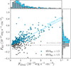 |
Fig. A.1. Flux distribution of [O III] and Hβ in our sample. The blue circles represent measurements with S/NHβ > 1.5, while the gray circles represent low-quality measurements with S/NHβ < 1.5. The blue dashed line marks the linear regression with the [O III]−Hβ relation, with the slope indicating the inverse of the median R3 ratio. Similar regression is applied to S/NHβ < 1.5 measurements, shown in the gray dashed line. No meaningful relations on R3 are constrained by those low-quality measurements. |
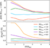 |
Fig. A.2. Bias of R3 ratios and metallicities from median stacking for simulated spectra with different SNRHβ. The different colors represent results with different input line ratios. |
Thus, we caution the potential bias of measuring line ratios for low S/N spectra even after median stacking. Such bias can be mitigated with higher S/N spectra.
Appendix B: Summary of sample properties
R3 diagnostics and inferred metallicity of in stacks of different subsets of our sample (with Hβ coverage at z > 5.5) split by stellar mass.
Comparison of the MZR with different studies in the literature. For measurements in this work, we show both the MZR measurements based on S24 and C24 calibrations.
In Table B.1, we provide the measured R3 ratios and the derived metallicities in different bins. In Table B.2 we list our measured MZR properties in comparison with measurements in the literature.
All Tables
Measurements of the median stack spectra for the full sample and subsets with [O III] and Hγ coverage at z > 6.25.
R3 diagnostics and inferred metallicity of in stacks of different subsets of our sample (with Hβ coverage at z > 5.5) split by stellar mass.
Comparison of the MZR with different studies in the literature. For measurements in this work, we show both the MZR measurements based on S24 and C24 calibrations.
All Figures
|
Fig. 1. Redshift distribution of the full sample in this work. [O III] emitters from ASPIRE and EIGER programs are marked by red and blue, respectively. The EIGER sample is stacked on top of the ASPIREsample. |
| In the text | |
|
Fig. 2. Median stacked 1D rest-frame spectra for our full sample galaxies at z > 6.25, with continuum subtracted. The fluxes are normalized by the peak of [O III]5007 flux after stacking. |
| In the text | |
|
Fig. 3. Mass–excitation diagram for our sample galaxies. The blue circles represent individual measurements. The red and blue diamonds represent stacked measurements in cluster and field galaxies, respectively. The blue and orange curves indicate the lower and upper mass-excitation demarcation by Coil et al. (2015). The AGNs (star-forming galaxies) are above (below) the demarcation. The gray shaded region indicates the high-mass end, which we did not analyze due to uncertainties in the metallicity calibrations in this regime. |
| In the text | |
|
Fig. 4. Mass–metallicity relation for galaxies in protoclusters (red) and blank fields (blue), which are based on R3 calibration from C24. The S24 calibration provides similar results, which are listed in the Table B.2 for comparison. The results from other works in the literature are shown with different colors, which are also listed in the Table B.2 for reference. Higher redshift (z > 3) measurements in literature are shown in solid lines, and lower redshift (z ∼ 2 − 3) measurements are shown in dashed lines. |
| In the text | |
|
Fig. 5. Metallicity offset between galaxies in overdense and field environments. The blue line shows the offset of MZR between cluster and field galaxies, with the shaded region representing a 1σ confidence interval. The single blue diamond shows the offset between the mass-matched cluster and field samples. The measurements in literature (Wang et al. 2022; Kacprzak et al. 2015; Sattari et al. 2021; Kulas et al. 2013; Chartab et al. 2021; Shimakawa et al. 2015; Valentino et al. 2015) are also shown for comparison, each marked in different colors. The error bars represent 1σ uncertainties. |
| In the text | |
|
Fig. 6. Offsets in metallicity between observations and the predictions of the local FMR with α = 0.66 (Andrews & Martini 2013). The orange and blue shadows represent the predictions in TNG and EAGLE simulation (Garcia et al. 2025). The offsets reported by Curti et al. (2024), Heintz et al. (2023) used a different FMR formalism, and we recalculated the offsets using Andrews & Martini (2013) formalism. For Nakajima et al. (2023), Sarkar et al. (2025), we added a constant offset of −0.2 dex to their FMR offsets to account for the systematic offset in metallicity calibrations used in their studies. |
| In the text | |
|
Fig. 7. Predicted Z − SFR relations for different model configurations. First panel: model 1, incorporating inflow but no outflow, with ϵSF as the varying parameter. Second panel: model 2, incorporating outflow but no inflow, with ϵSF as the varying parameter. Third panel: model 3, incorporating both inflow and outflow, with η as the varying parameter. Fourth panel: model 4, incorporating both inflow and outflow, with β as the varying parameter. In all panels, the lines are color-coded by stellar mass, while different line styles indicate variations in model parameters. |
| In the text | |
|
Fig. 8. Top: predicted MZR for galaxies with different tobs. The dashed lines are MZRs color-coded by tobs. This model assumes ϵSF = 0.02, η0 = 5, and an energy-driven wind β = 2/3. The diamond points are our observations, the same as in Fig. 4. Bottom: Predicted SFR−Z relation for galaxies is shown for different stellar masses and tobs. The dashed lines, color-coded by tobs, connect galaxies with the same observational time, while the solid black lines link galaxies of equal stellar mass. Different stellar masses are represented by different symbols. The red and blue diamond points are our observations in cluster and field environments. The asymmetric errors on SFR are due to uncertainties in dust correction. |
| In the text | |
|
Fig. 9. Observed MZR compared with hydrodynamical simulations. The symbols for our observations are the same as in Fig. 4. The results at similar redshifts from different suites of hydrodynamical simulations are denoted by different colors, including FIRSTLIGHT (Langan et al. 2020), FIRE (Ma et al. 2016), FIRE-2 (Marszewski et al. 2024), ILLUSTRISTNG (Torrey et al. 2019), and ASTRAEUS (Ucci et al. 2023). |
| In the text | |
|
Fig. A.1. Flux distribution of [O III] and Hβ in our sample. The blue circles represent measurements with S/NHβ > 1.5, while the gray circles represent low-quality measurements with S/NHβ < 1.5. The blue dashed line marks the linear regression with the [O III]−Hβ relation, with the slope indicating the inverse of the median R3 ratio. Similar regression is applied to S/NHβ < 1.5 measurements, shown in the gray dashed line. No meaningful relations on R3 are constrained by those low-quality measurements. |
| In the text | |
|
Fig. A.2. Bias of R3 ratios and metallicities from median stacking for simulated spectra with different SNRHβ. The different colors represent results with different input line ratios. |
| In the text | |
Current usage metrics show cumulative count of Article Views (full-text article views including HTML views, PDF and ePub downloads, according to the available data) and Abstracts Views on Vision4Press platform.
Data correspond to usage on the plateform after 2015. The current usage metrics is available 48-96 hours after online publication and is updated daily on week days.
Initial download of the metrics may take a while.